Linear Convergence Results for Inertial Type Projection Algorithm for Quasi-Variational Inequalities

Abstract

Many recently proposed gradient projection algorithms with inertial extrapolation step for solving quasi-variational inequalities in Hilbert spaces are proven to be strongly convergent with no linear rate given when the cost operator is strongly monotone and Lipschitz continuous. In this paper, our aim is to design an inertial type gradient projection algorithm for quasi-variational inequalities and obtain its linear rate of convergence. Therefore, our results fill in the gap for linear convergence results for inertial type gradient projection algorithms for quasi variational inequalities in Hilbert spaces. We perform numerical implementations of our proposed algorithm and give numerical comparisons with other related inertial type gradient projection algorithms for quasi variational inequalities in the literature.

Keywords: Quasi-variational inequalities; gradient projection algorithm; inertial extrapolation; strongly Monotone.

2010 MSC classification: 47H05, 47J20, 47J25, 65K15, 90C25.

1 Introduction

Suppose that $H$ is a real Hilbert space equipped with inner product $\langle\cdot,\cdot\rangle$ and induced norm $\|\cdot\|$. Assume further that $K$ is a nonempty, closed and convex subset of $H$. Given a nonlinear operator $\mathcal{A}:H\rightarrow H$ and a set-valued operator $K:H\rightrightarrows H$ such that for each element $x\in H$, we have a closed and convex set $K(x)\subset H$. Then the Quasi-Variational Inequality (QVI), is to find $x_{*}\in H$ such that $x_{*}\in K(x_{*})$ and

$$\left\langle\mathcal{A}(x_{*}),x-x_{*}\right\rangle\geq 0\text{ for all }x\in K(x_{*}).$$ (1)

In the special case when $K(x)\equiv K$ for all $x\in H$, we have the QVI (1) reduces to the variational inequality problem ([21, 22, 44, 28]), viz.: find $x_{*}\in K$ such that

$$\left\langle\mathcal{A}(x_{*}),x-x_{*}\right\rangle\geq 0\text{ for all }x\in K.$$ (2)

Several projection type methods have been introduced to solve QVI (1) in the literature. In [3], Antipin et al. designed the gradient projection algorithm:

$$x_{k+1}=P_{K(x_{k})}(x_{k}-\gamma\mathcal{A}(x_{k}))$$ (3)

and the extragradient algorithm:

$$\left\{\begin{array}[]{ll}&y_{k}=P_{K(x_{k})}(x_{k}-\gamma\mathcal{A}(x_{k})),\\ &x_{k+1}=P_{K(x_{k})}(x_{k}-\gamma\mathcal{A}(y_{k}))\end{array}\right.$$ (6)

to solve QVI (1) and obtained strong convergence results when $K(x):=c(x)+K$, $c$ Lipschitz continuous, $\mathcal{A}$ is strongly monotone and Lipschitz continuous. Similar results to [3] are also obtained in [33, 35, 36, 37].

We note that the extragradient method (6) requires computing two projections and two evaluations of $\mathcal{A}$ per iteration. This could be computational expensive for large scale problems. In [32], Mijajlović et al. introduced relaxed projection type algorithms

$$x_{k+1}=(1-\alpha_{k})x_{k}+\alpha_{k}P_{K(x_{k})}(x_{k}-\gamma\mathcal{A}(x_{k}))$$ (7)

and

$$\left\{\begin{array}[]{ll}&y_{k}=(1-\beta_{k})x_{k}+\beta_{k}P_{K(x_{k})}(x_{k}-\gamma\mathcal{A}(x_{k})),\\ &x_{k+1}=(1-\alpha_{k})x_{k}+\alpha_{k}P_{K(y_{k})}(y_{k}-\gamma\mathcal{A}(y_{k}))\end{array}\right.$$ (10)

where $\alpha_{k}\in(0,1],\beta_{k}\in[0,1]$. Consequently, strong convergence results are obtained for QVI (1) when $\mathcal{A}$ is strongly monotone and Lipschitz continuous operator with condition (19) fulfilled for which the case $K(x):=c(x)+K,x\in H$ satisfies. The proposed algorithm in (3) is a special case of algorithm (7) with $\alpha_{k}=1$ and the results of Mijajlović et al. [32] are also related to the ones in [8, 18, 19, 29].

Due to recent contributions of optimization algorithms with inertial extrapolation steps in terms of improvement on the speed of convergence as enumerated in [5, 6, 1, 2, 9, 31, 40, 7, 30, 39, 10, 42, 11, 15, 12] and other related papers, gradient projection algorithms with extrapolation step for solving QVI (1) was studied in [43]:

$$\left\{\begin{array}[c]{ll}&y_{k}=x_{k}+\theta_{k}(x_{k}-x_{k-1}),\\ &x_{k+1}=(1-\alpha_{k})y_{k}+\alpha_{k}P_{K(y_{k})}(y_{k}-\gamma\mathcal{A}(y_{k})),\end{array}\right.$$ (13)

with $\alpha_{k}\in(0,1)$ and $0\leq\theta_{k}\leq\theta<1$ and strong convergence results (with no linear convergence results) obtained under condition that $\mathcal{A}$ is strongly monotone and Lipschitz continuous. With $\mathcal{A}$ being strongly monotone and Lipschitz continuous in QVI (1), C̣opur et al. in [16] also obtained strong convergence results for the gradient projection algorithm (3) with double inertial extrapolation steps. However, no linear convergence results was also given in [16]. Similar strong convergence results with no linear rate of convergence are given in [27].

Our Contributions.

• Motivated by the inertial type gradient projection algorithms proposed in [16, 27, 43], where no linear convergence results are given, our aim in this paper is to prove the linear convergence of an inertial type projection algorithm for QVI (1).

• The inertial factor in our proposed algorithm has the possibility of taking both negative and non-negative values unlike the inertial factors in [16, 27, 43] and other associated papers where the inertial factors are in [0,1]. Kindly see Remark 3.2 below.

• We also show that proposed inertial type gradient projection algorithm proposed in this paper is efficient and outperforms the other related inertial type gradient projection algorithms in [16, 42, 43] using standard test problems in the literature.

Outline. We outline the paper as, viz: Section 2 entails some basic facts, concepts, and lemmas, which are needed in the linear convergence analysis. In Section 3, we introduce an inertial type gradient projection algorithm with their corresponding linear convergence results given. Section 4 discusses the numerical implementations of the proposed algorithm with comparisons with other related algorithms while in Section 5, we give a final conclusion of our results.

2 Preliminaries

Definition 2.1.

Given an operator $\mathcal{A}:H\rightarrow H$,

• $\mathcal{A}$ is called $L$-Lipschitz continuous ($L>0$), if

  $$\|\mathcal{A}(x)-\mathcal{A}(y)\|\leq L\|x-y\|\text{ for all }x,y\in H.$$ (14)

• $\mathcal{A}$ is called $\mu$-strongly monotone ($\mu>0$), if

  $$\langle\mathcal{A}(x)-\mathcal{A}(y),x-y\rangle\geq\mu\|x-y\|^{2}\text{ for all }x,y\in H.$$ (15)

For each $x\in H$, there exists a unique nearest point in $K$, denoted by $P_{K}(x)$, such that

$$\|x-P_{K}(x)\|\leq\|x-y\|\text{ for all }y\in K.$$ (16)

This operator $P_{K}:H\rightarrow K$ is called the metric projection of $H$ onto $K$, characterized [26, Section 3] by

$$P_{K}(x)\in K$$ (17)

and

$$\left\langle x-P_{K}\left(x\right),P_{K}\left(x\right)-y\right\rangle\geq 0\text{ for all }x\in H,\text{ }y\in K.$$ (18)

We state the following sufficient conditions for the existence of solutions of QVIs (1) given in [38].

Lemma 2.2.

Let $\mathcal{A}:H\rightarrow H$ be $L$-Lipschitz continuous and $\mu$-strongly monotone on $H$ and $K(\cdot)$ be a set-valued mapping with nonempty, closed and convex values such that there exists $\lambda\geq 0$ such that

$$\|P_{K(x)}(z)-P_{K(y)}(z)\|\leq\lambda\|x-y\|,\leavevmode\nobreak\ \leavevmode\nobreak\ x,y,z\in H,\quad\lambda+\sqrt{1-\frac{\mu^{2}}{L^{2}}}<1.$$ (19)

Then the QVI (1) has a unique solution.

The fixed point formulation of the QVI (1) is given by

Lemma 2.3.

Let $K(\cdot)$ be a set-valued mapping with nonempty, closed and convex values in $H$. Then $x_{*}\in K(x_{*})$ is a solution of the QVI (1) if and only if for any $\gamma>0$ it holds that

$$x_{*}=P_{K(x_{*})}(x_{*}-\gamma\mathcal{A}(x_{*})).$$

The following lemma is needed in our convergence analysis.

Lemma 2.4.

If $x,y\in H$, we have

• $2\langle x,y\rangle=\|x\|^{2}+\|y\|^{2}-\|x-y\|^{2}=\|x+y\|^{2}-\|x\|^{2}-\|y\|^{2}.$

• Assume that $x,y\in H$ and $\alpha\in\mathbb{R}$. Then

  $$\|\alpha x+(1-\alpha)y\|^{2} = \alpha\|x\|^{2}+(1-\alpha)\|y\|^{2}-\alpha(1-\alpha)\|x-y\|^{2}.$$

3 Main Results

We introduce our inertial type gradient projection algorithm for solving QVI (1) and obtain linear convergence results. To begin with, let us assume that a parameter $\gamma\geq 0$ obeys the following condition:

Assumption 3.1.

$$\left|\gamma-\frac{\mu}{L^{2}}\right|<\frac{\sqrt{\mu^{2}-L^{2}\lambda(2-\lambda)}}{L^{2}}.$$ (20)

We now introduce an inertial type projection algorithm for solving the QVI (1).

Algorithm 1 Inertial Type Gradient Projection Algorithm

1:Choose $\theta_{k}\in(0,1)$ such that $0<a\leq\theta_{k}\leq b<1$ and pick $z_{-1}=z_{0}\in H.$ Set $k:=0$.

2:Given the current iterates $z_{k-1}$ and $z_{k},$ compute

$$\left\{\begin{array}[]{ll}&y_{k-1}=z_{k}+\Big{(}\frac{1-2\theta_{k-1}}{\theta_{k-1}}\Big{)}(z_{k}-z_{k-1}),\\ &x_{k}=P_{K(y_{k-1})}(y_{k-1}-\gamma\mathcal{A}(y_{k-1})),\\ &z_{k+1}=(1-\theta_{k})z_{k}+\theta_{k}x_{k}\end{array}\right.$$ (24)

3:Set $k\leftarrow k+1$, and return to 2.

Remark 3.2.

 
(a) Our proposed inertial-type gradient projection Algorithm 1 features an inertial factor $\frac{1-2\theta_{k-1}}{\theta_{k-1}}\in(-1,+\infty)$. In particular, if $\theta_{k-1}\in(\frac{1}{2},1)$ in Algorithm 1, the inertial factor $\frac{1-2\theta_{k-1}}{\theta_{k-1}}\in(-1,0)$, while if $\theta_{k-1}\in(0,\frac{1}{2})$ in Algorithm 1, the inertial factor $\frac{1-2\theta_{k-1}}{\theta_{k-1}}\in(0,+\infty)$. Therefore, the inertial term in our algorithm 1 is not restricted to $[0,1]$, which was considered in other inertial-type projection algorithms proposed and studied in [16, 27, 42, 43].

(b) If $\theta_{k}=\frac{1}{3}$ in Algorithm 1, then Algorithm 1 becomes an averaging reflected gradient projection algorithm, which is a similar algorithm studied in [42].

We now give our linear convergence results for Algorithm 1.

Theorem 3.3.

Consider the QVI (1) with $\mathcal{A}$ being $\mu$-strongly monotone and $L$-Lipschitz continuous and assume there exists $\lambda\geq 0$ such that (19) holds. Let $\{x_{k}\}$ and $\{z_{k}\}$ be generated by Algorithm 1 with $\gamma\geq 0$ satisfying (20). Then both $\{x_{k}\}$ and $\{z_{k}\}$ converge linearly to the unique solution $x_{*}\in K(x_{*})$ of the QVI (1).

Proof.

We obtain from Algorithm 1 that

$$y_{k} = z_{k+1}+\Big{(}\frac{1-2\theta_{k}}{\theta_{k}}\Big{)}(z_{k+1}-z_{k})$$ (25)

$$= (1-\theta_{k})z_{k}+\theta_{k}x_{k}+\theta_{k}\Big{(}\frac{1-2\theta_{k}}{\theta_{k}}\Big{)}(x_{k}-z_{k})$$

$$= (1-\theta_{k})z_{k}+\theta_{k}x_{k}+(1-2\theta_{k})(x_{k}-z_{k})$$

$$= \Big{(}(1-\theta_{k})-(1-2\theta_{k})\Big{)}z_{k}+(\theta_{k}+1-2\theta_{k})x_{k}$$

$$= (1-\theta_{k})x_{k}+\theta_{k}z_{k}.$$

Now, given the unique solution $x_{*}$ of (1), we obtain

$$\|x_{k+1}-x_{*}\| = \|P_{K(y_{k})}(w_{k}-\gamma\mathcal{A}(y_{k}))-P_{K(x_{*})}(x_{*}-\gamma\mathcal{A}(x_{*}))\|$$ (26)

$$\leq \|P_{K(y_{k})}(w_{k}-\gamma\mathcal{A}(y_{k}))-P_{K(x_{*})}(y_{k}-\gamma\mathcal{A}(y_{k}))\|$$

$$+\|P_{K(x_{*})}(y_{k}-\gamma\mathcal{A}(y_{k}))-P_{K(x_{*})}(x_{*}-\gamma\mathcal{A}(x_{*}))\|$$

$$\leq \lambda\|y_{k}-x_{*}\|+\|y_{k}-x_{*}+\gamma(\mathcal{A}(x_{*})-\mathcal{A}(y_{k}))\|.$$

By the fact that $\mathcal{A}$ is $\mu$-strongly monotone and $L-$Lipschitz continuous, we obtain

$$\|y_{k}-x_{*}-\gamma(\mathcal{A}(x_{*})-\mathcal{A}(y_{k}))\|^{2} = \|y_{k}-x_{*}\|^{2}-2\gamma\langle\mathcal{A}(y_{k})-\mathcal{A}(x_{*}),y_{k}-x_{*}\rangle$$ (27)

$$+\gamma^{2}\|\mathcal{A}(y_{k})-\mathcal{A}(x_{*})\|^{2}$$

$$\leq (1-2\mu\gamma+\gamma^{2}L^{2})\|y_{k}-x_{*}\|^{2}.$$

Combining (26) and (27), we get

$$\|x_{k+1}-x_{*}\| \leq \lambda\|y_{k}-x_{*}\|+\sqrt{1-2\mu\gamma+\gamma^{2}L^{2}}\|y_{k}-x_{*}\|$$ (28)

$$= \beta\|y_{k}-x_{*}\|,$$

with

$$\beta:=\sqrt{1-2\mu\gamma+\gamma^{2}L^{2}}+\lambda\in(0,1).$$ (29)

By (25) and Lemma 2.4, we obtain

$$\|y_{k}-x_{*}\|^{2} = \|(1-\theta_{k})(x_{k}-x_{*})+\theta_{k}(z_{k}-x_{*})\|^{2}$$ (30)

$$= (1-\theta_{k})\|x_{k}-x_{*}\|^{2}+\theta_{k}\|z_{k}-x_{*}\|^{2}$$

$$-\theta_{k}(1-\theta_{k})\|x_{k}-z_{k}\|^{2}$$

and

$$\|z_{k+1}-x_{*}\|^{2} = \|(1-\theta_{k})(z_{k}-x_{*})+\theta_{k}(x_{k}-x_{*})\|^{2}$$ (31)

$$= (1-\theta_{k})\|z_{k}-x_{*}\|^{2}+\theta_{k}\|x_{k}-x_{*}\|^{2}$$

$$-\theta_{k}(1-\theta_{k})\|x_{k}-z_{k}\|^{2}.$$

By these last two identities, we obtain from (28) that

$$\|x_{k+1}-x_{*}\|^{2}+\|z_{k+1}-x_{*}\|^{2} \leq \beta^{2}\|y_{k}-x_{*}\|^{2}$$ (32)

$$+(1-\theta_{k})\|z_{k}-x_{*}\|^{2}+\theta_{k}\|x_{k}-x_{*}\|^{2}$$

$$-\theta_{k}(1-\theta_{k})\|x_{k}-z_{k}\|^{2}$$

$$= (1-\theta_{k})\beta^{2}\|x_{k}-x_{*}\|^{2}+\theta_{k}\beta^{2}\|z_{k}-x_{*}\|^{2}$$

$$-\beta^{2}\theta_{k}(1-\theta_{k})\|x_{k}-z_{k}\|^{2}$$

$$+(1-\theta_{k})\|z_{k}-x_{*}\|^{2}+\theta_{k}\|x_{k}-x_{*}\|^{2}$$

$$-\theta_{k}(1-\theta_{k})\|x_{k}-z_{k}\|^{2}$$

$$= \beta^{2}\Big{(}\|x_{k}-x_{*}\|^{2}+\|z_{k}-x_{*}\|^{2}\Big{)}$$

$$+\theta_{k}(1-\beta^{2})\|x_{k}-x_{*}\|^{2}+(1-\theta_{k}(1-\beta^{2})\|z_{k}-x_{*}\|^{2}$$

$$-\theta_{k}(1-\theta_{k})(1+\beta^{2})\|x_{k}-z_{k}\|^{2}$$

$$\leq \beta^{2}\Big{(}\|x_{k}-x_{*}\|^{2}+\|z_{k}-x_{*}\|^{2}\Big{)}$$

$$+\theta_{k}(1-\beta^{2})\|x_{k}-x_{*}\|^{2}+(1-\beta^{2})(1-\theta_{k})\|z_{k}-x_{*}\|^{2}$$

$$\leq \beta^{2}\Big{(}\|x_{k}-x_{*}\|^{2}+\|z_{k}-x_{*}\|^{2}\Big{)}$$

$$+\theta_{k}(1-\beta^{2})\Big{(}\|x_{k}-x_{*}\|^{2}+\|z_{k}-x_{*}\|^{2}\Big{)}$$

$$+(1-\beta^{2})(1-\theta_{k})\Big{(}\|x_{k}-x_{*}\|^{2}+\|z_{k}-x_{*}\|^{2}\Big{)}$$

$$\leq \beta^{2}\Big{(}\|x_{k}-x_{*}\|^{2}+\|z_{k}-x_{*}\|^{2}\Big{)}$$

$$+b(1-\beta^{2})\Big{(}\|x_{k}-x_{*}\|^{2}+\|z_{k}-x_{*}\|^{2}\Big{)}$$

$$+(1-\beta^{2})(1-a)\Big{(}\|x_{k}-x_{*}\|^{2}+\|z_{k}-x_{*}\|^{2}\Big{)}$$

$$= \varrho\Big{(}\|x_{k}-x_{*}\|^{2}+\|z_{k}-x_{*}\|^{2}\Big{)},$$

where

$$\varrho:=\max\Big{\{}\beta^{2},b(1-\beta^{2}),(1-\beta^{2})(1-a)\Big{\}}\in(0,1).$$

Consequently,

$$\|x_{k+1}-x_{*}\|^{2} \leq \|x_{k+1}-x_{*}\|^{2}+\|z_{k+1}-x_{*}\|^{2}$$ (33)

$$\leq \varrho\Big{(}\|x_{k}-x_{*}\|^{2}+\|z_{k}-x_{*}\|^{2}\Big{)}$$

$$\leq \varrho^{k+1}\Big{(}\|x_{0}-x_{*}\|^{2}+\|z_{0}-x_{*}\|^{2}\Big{)}$$

$$= 2\varrho^{k+1}\|x_{0}-x_{*}\|^{2}.$$

Hence, $\{x_{k}\}$ converges linearly to the unique solution $x_{*}\in K(x_{*})$ of the QVI (1). We can also show from (33) that $\{z_{k}\}$ also converges linearly to the unique solution $x_{*}\in K(x_{*})$ of the QVI (1) since

$$\|z_{k+1}-x_{*}\|^{2} \leq \|x_{k+1}-x_{*}\|^{2}+\|z_{k+1}-x_{*}\|^{2}$$ (34)

$$\leq 2\varrho^{k+1}\|x_{0}-x_{*}\|^{2}.$$

∎

In a special case when $K(x),x\in H$ is a ”moving set”. That is, the case when $K(x):=c(x)+K,x\in H$ where $c:H\rightarrow H$ is a $\lambda$-Lipschitz continuous mapping and $K\subset H$ is a nonempty, closed and convex subset. Then the Assumption (20) is automatically satisfied with the same value of $\lambda$ (see [34]). The following result hold in this case.

Corollary 3.4.

Consider the QVI (1) with $\mathcal{A}$ being $\mu$-strongly monotone and $L$-Lipschitz continuous and suppose that $K(x):=c(x)+K,x\in H$ where $c:H\rightarrow H$ is a $\lambda$-Lipschitz continuous mapping and $K$ is a nonempty, closed and convex subset of $H$. Let $\{x_{k}\}$ be any sequence generated by Algorithm 1 with $\gamma\geq 0$ satisfying (20). Then $\{x_{k}\}$ and $\{z_{k}\}$ converge linearly to the unique solution $x_{*}\in K(x_{*})$ of the QVI (1).

Remark 3.5.

 
(a) In the inertial type gradient projection algorithms proposed in [16, 27, 43], only strong convergence results are obtained with no linear rate of convergence discussed. In this paper, we propose an inertial type gradient projection algorithm with linear convergence results given.

(b) In the case when $\theta_{k}=\frac{1}{2}$ in our Algorithm 1, our algorithm becomes a special case of the algorithms studied in [32, 43].

4 Numerical Examples

We give some numerical implementations of our proposed Algorithm 1 and give comparisons with some existing methods in the literature. All codes were written in MATLAB R2023a and performed on a PC Desktop Intel Core i5-8265U CPU 1.60GHz 1.80 GHz, RAM 16.00GB. We compare Algorithm 1 with the proposed algorithms in [3, 16, 42, 43].

We choose to use the test problem library QVILIB taken from [20]; the feasible map $K$ is assumed to be given by $K(x):=\{z\in\mathbb{R}^{n}\,:\,g(z,x)\leq 0\}$. We implemented Algorithm 1 in Matlab. We implemented the projection over a convex set as the solution of a convex program. We considered the following performance measures for optimality and feasibility

$$\text{opt}(x):=-\min_{z}\{{\cal F}(x)^{T}(z-x)\,:\,z\in K(x)\},\;\;\text{feas}(x):=\|\max\{0,g(x,x)\}\|_{\infty}.$$

A point $x^{*}$ is considered a solution of the QVI if the optimality measure opt$(x^{*})\leq 1e$-4 and feasibility measure feas$(x^{*})\leq 1e$-4. For solving the QVI, we utilized the built-in function fmincon with ‘sqp’ algorithm as its internal method, setting the maximum iteration count to 1000. The QVILIB [20] provides a comprehensive collection of test problems specifically designed for evaluating algorithms employed in solving QVI. These problems encompasses a wide range of scenarios, including academic models, real-world applications and discretized versions of infinite-dimensional QVIs that model various engineering and physical phenomena. Furthermore, the library offers an M-file named startinPoints, which facilitates obtaining initial strating points for each test problem. The feasible set $K(x)$ is defined as the intersection of a fixed set $\bar{K}$ and a moving set $\tilde{K}(x)$ that depends on the point $x$ given by:

$$\bar{K} := \{y\in\mathbb{R}^{k}\;|\;g^{I}(y)\leq 0,\;M^{I}y+v^{I}=0\},$$

$$\tilde{K}(x) = \{y\in\mathbb{R}^{k}\;|\;g^{P}(y,x)\leq 0,\;M^{P}(x)y+v^{P}(x)=0\}.$$

The comprehensive definitions of each problem can be found in [20]; however, we provide a brief description of each problem in Table 1.

Table 1: Description of test problems used in the experiments

Problem name	$n$	$m_{I}$	$p_{I}$	$m_{P}$	$p_{P}$	n(start)
OutZ40	2	4	0	2	0	3
OutZ41	2	4	0	2	0	3
OutZ42	4	4	0	4	0	4
OutZ43	4	0	0	4	0	3
OutZ44	4	0	0	4	0	3
MovSet1A	5	0	0	1	0	2
MovSet1B	5	0	0	1	0	2
MovSet2A	5	0	0	1	0	2
MovSet2B	5	0	0	1	0	2
Box1A	5	0	0	10	0	2
Box1B	5	0	0	10	0	2
BiLin1A	5	10	0	3	0	2
BiLin1B	5	10	0	3	0	2
WalEq1	18	18	1	5	0	2
WalEq2	105	105	1	20	0	2
WalEq3	186	186	1	30	0	2
WalEq4	310	310	1	30	0	2
WalEq5	492	492	1	40	0	2
Wal2	105	107	0	20	0	2
Wal3	186	188	0	30	0	2
LunSSVI1	501	1002	1	0	0	2
OutKZ41	82	82	0	82	0	2

In Table 1, the first column contains the name of the problem, the second column ($n$) contains the number of variables in the problem, column $m_{I}$ contains the number of inequality constraints defining $\bar{K}$, column $p_{I}$ contains the number of linear equalities in $\bar{K},$ the column $m_{P}$ contains the number of inequality constraints defining $\tilde{K}(x)$, the column the $p_{P}$ is the number of equalities in the definition of $\tilde{K}(x)$ and the last column n(start) is the number of starting points for the problem.

In order to compare the performance of the algorithms, we used the so-called performance profiles, see [17], based on the number of iterations and execution time of the algorithm. Let $t_{s,i}>0$ denote the comparison metric (related to the current performance index) of solver $s\in\mathcal{S}$ for addressing instance $i\in\mathcal{I}$ of the problem, where $\mathcal{S}$ represents the set of comparing algorithms and $\mathcal{I}$ denotes the various problems with different starting points. We define the performance ratio by

$$\forall s\in\mathcal{S},\,\forall i\in\mathcal{I}\colon\quad r_{s,i}:=\dfrac{t_{s,i}}{\min\{t_{s^{\prime},i}\,|\,s^{\prime}\in\mathcal{S}\}}.$$

This quantity is called the ratio of the performance of solver $s\in\mathcal{S}$ to solve problem $i\in\mathcal{I}$ compared to the best performance of any other algorithm in $\mathcal{S}$ to solve problem $i$. The cumulative distribution function $\rho_{s}\colon[1,\infty)\to[0,1]$ of the current performance index linked with solver $s\in\mathcal{S}$ is defined as follows:

$$\forall\tau\in[1,\infty)\colon\quad\rho_{s}(T):=\frac{|\{i\in\mathcal{I}\,|\,r_{s,i}\leq T\}|}{|\mathcal{I}|}.$$

The performance profile for a specific performance index displays the graphical representations of all the functions $\rho_{s}$, where $s$ varies across the set $\mathcal{S}$. The value $\rho_{s}(1)$ indicates the proportion of problem instances where solver $s\in\mathcal{S}$ exhibits the best performance. For any arbitrary $\tau\geq 1$, $\rho_{s}(T)$ represents the fraction of problem instances where solver $s\in\mathcal{S}$ achieves at most $T$ times the best performance.

In our experiments, we choose the following control parameters for the algorithms:

• Proposed Alg: $\gamma=0.5,\theta_{k}=\frac{k}{5(k+1)};$

• Antipin et al. Alg: $\gamma=0.5;$

• Mijajlovic et al Alg. 1: $\gamma=0.5,\alpha_{k}=\frac{1}{k+1};$

• Mijajlovic et al. Alg. 2: $\gamma=0.5,\alpha_{k}=\frac{1}{k+1},\beta_{k}=\frac{3k}{7k+9};$

• Shehu et al Alg: $\gamma=0.5,\theta_{k}=\frac{k}{5(k+1)},\alpha_{k}=\frac{1}{k+1}.$

Figure 1 provides a comprehensive view of the performance profile analysis, focusing on the number of iterations required by each algorithm. The result highlights the proposed Algorithm as the standout performer, demonstrating superior efficiency with the least number of iterations across nearly 82% of the experimental scenarios. This suggests that the proposed Algorithm consistently converges more rapidly compared to its counterparts, making it a compelling choice for solving the QVI problems. In comparison, the Shehu et al Algorithm emerges as the second-best performer, showcasing the best performance in approximately 64% of the experiments. While not as dominant as the proposed Algorithm, it shares similar number of iterations with the proposed algorithm in significant number of cases. Furthermore, the Antipin et al Algorithm achieves the best performance in roughly 57% of the experiments, the Mijajlovic et al Algorithm 2 has best performance in 53% of the experiments, while Mijajlovic et al Algorithm 1 has best performance in about 51% of the experimental scenarios. This is collaborated with the average results shown in Table 2. Although Antinpin et al. Alg has lower average number of iteration than Mijajlovic et al Alg 1 and 2, this is because Antipin et al. Alg. has smaller figures at instances it achieved successes compare to the Mijajlovic et al algorithms.

Figure 2 shows the performance profile of the algorithm based on the time of execution. The result shows that the proposed algorithm has the least time of execution for about 45% of the scenarios. This is follow by Shehu et al algorithm which shares very closed figures with the rest of the comparing algorithms. This further highlights the advantage of the proposed algorithm over the rest of the algorithms. The average execution time presented in Table 2 indicates that the Antipin et al Algorithm exhibits the longest average execution time. This outcome aligns with expectations, as the Antipin et al. Algorithm involves computing two projections per iteration utilizing the optimization solver, which inherently consumes additional computational resources. Similarly, the Mijajlovic et al Algorithm 2 also computes two projections in each iteration, contributing to a higher average execution time. However, it’s worth noting that in this case, the output is regularized by the control parameters $\alpha_{k}$ and $\beta_{k}$, which may mitigate some of the computational overhead associated with the additional projections.

Figure 3 shows the number of instances the algorithm terminate due to the stopping criterion. Recall that the algorithm is terminated if a solution of the QVI problem is found (Termination 1) or the computation reaches the maximum iteration (Termination 2). From Figure 3, we observe that the Proposed Algorithm terminated due to Termination 1 in 39 instances, which accounts for approximately 88.6% of the total cases. Similarly, Mijajlovic et al. Algorithms 1 and 2, along with Antipin et al. Algorithm, stopped due to Termination 1 in 37 instances, representing 84.1% of the experiments. Additionally, the Shehu et al. Algorithm reached Termination 1 in 36 instances, constituting about 81.8% of the total scenarios. These findings underscore the computational advantage of the Proposed Algorithm, as it consistently terminates due to finding a solution to the QVI problem in a higher proportion of instances compared to the other algorithms. This also suggests that the Proposed Algorithm converges more efficiently, leading to quicker termination based on achieving the desired solution.

Figure 4 shows the result of the experimental order of convergence (EOC) of each algorithm. The EOC is calculated by computing

$$EOC:=\max\left(\frac{\log\|x_{k+1}-x_{k}\|}{\log\|x_{k}-x_{k-1}\|},\frac{\log\|x_{k+2}-x_{k+1}\|}{\log\|x_{k+1}-x_{k}\|}\right).$$

This formula provides an estimation of how quickly the error (or performance measure) decreases as the algorithm progresses. A higher value of EOC indicates faster convergence. From Figure 4, we observe that the proposed algorithm achieves the highest EOC value in 11 instances. In 31 instances, it shares equivalent EOC values with other algorithms, indicating comparable convergence rates. However, in 2 instances, the proposed algorithm exhibits a lower EOC value. Interestingly, Mijajlovic et al Algorithm 2 attains the highest EOC value in only 1 instance. This outlier occurrence could potentially be attributed to the influence of regularization parameters integrated within the algorithm, which may have impacted its convergence behavior in this particular case.

Table 2: Summary of numerical results

	Av. Iter	Av. Time	# Feas sol.	# No Feas. sol.
Proposed Alg.	4.5455	4.6086	39	5
Mijajlovic et al Alg. 1	6.7045	8.5337	37	7
Mijajlovic et al Alg. 2	7.3863	14.8086	37	7
Shehu et al Alg.	6.1818	6.2171	36	8
Antipin et al Alg.	7.8409	18.2486	37	7

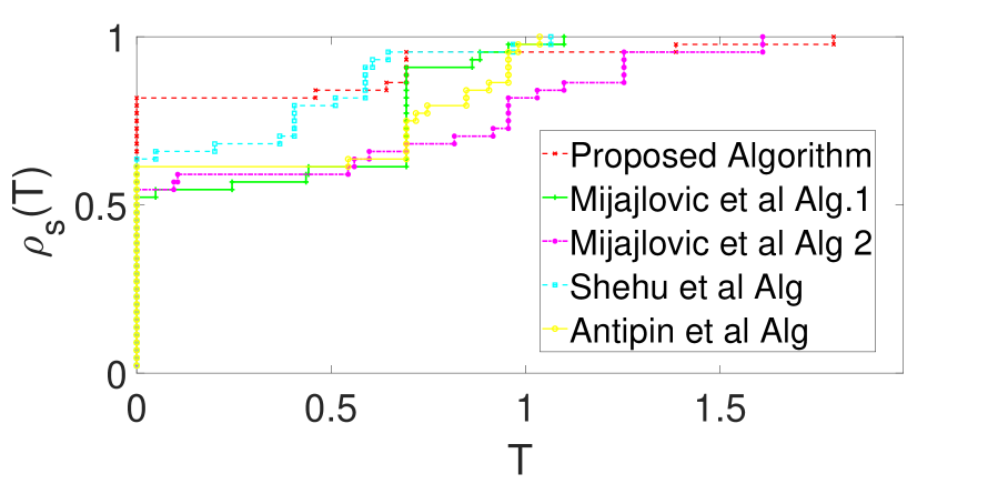
Figure 1: Performance profile based on number of iterations

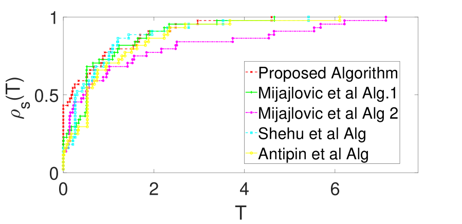
Figure 2: Performance profile based on the time of execution

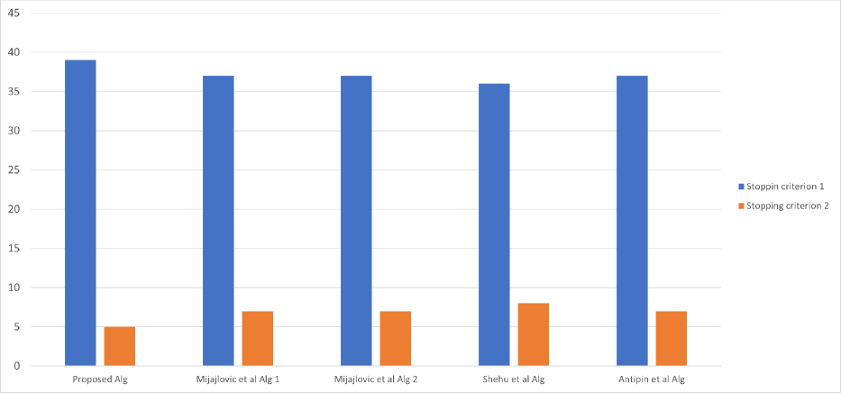
Figure 3: Numerical results showing the feasibility of solution based on the reason of termination

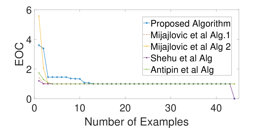
Figure 4: Experimental order of convergence of algorithms

5 Conclusion

In this paper, we introduced an inertial type gradient projection algorithm for solving quasi-variational inequalities in Hilbert spaces and obtain its linear convergence rate under strong monotonicity of the operator. This result complements other results in the literature for inertial type gradient projection algorithms to solve quasi-variational inequalities where only strong convergence results are obtained. We also showed that the inertial factor in our proposed inertial type gradient projection algorithm could take both negative and non-negative values unlike many other inertial type gradient projection algorithms for quasi-variational inequalities in the literature. The numerical comparisons of the proposed algorithm showed that our proposed inertial type gradient projection algorithm is efficient and outperform some popular related inertial type gradient projection algorithms in the literature for quasi-variational inequalities.

Disclosure statement

Ethical Approval and Consent to participate

All the authors gave ethical approval and consent to participate in this article.

Consent for publication

All the authors gave consent for the publication of identifiable details to be published in the journal and article.

Code availability

The Matlab codes employed to run the numerical experiments are available on request.

Availability of supporting data

Data sharing is not applicable to this article as no datasets were generated or analyzed during the current study.

Competing interests

The authors declare no competing interests.

Funding

Not Applicable.

Authors’ contributions

Y.Y. and Y.S. wrote the manuscript and L.O.J. prepared the all the figures and tables.

Acknowledgments

Not Applicable.

References

- [1] Alvarez, F.: Weak convergence of a relaxed and inertial hybrid projection-proximal point algorithm for maximal monotone operators in Hilbert space. SIAM J. Optim. 14, 773–782 (2003)
- [2] Alvarez, F., Attouch, H.: An inertial proximal method for maximal monotone operators via discretization of a nonlinear oscillator with damping. Set-Valued Anal. 9, 3–11 (2001)
- [3] Antipin, A. S., Jaćimović, M., Mijajlovi, N.: Extragradient method for solving quasivariational inequalities. Optimization 67, 103–112 (2018)
- [4] Antipin, A. S., Jaćimović, M., Mijajlovi, N.: A second-order iterative method for solving quasi-variational inequalities. Comp. Math. Math. Phys. 53, 258–264 (2013)
- [5] Attouch, H., Goudon, X., Redont, P.: The heavy ball with friction. I. The continuous dynamical system. Commun. Contemp. Math. 2, 1–34 (2000)
- [6] Attouch, H., Czarnecki, M. O.: Asymptotic control and stabilization of nonlinear oscillators with non-isolated equilibria. J. Diff. Equations 179, 278–310 (2002)
- [7] Attouch, H., Peypouquet, J., Redont, P.: A dynamical approach to an inertial forward-backward algorithm for convex minimization. SIAM J. Optim. 24, 232–256 (2014)
- [8] Aussel, D., Sagratella, S.: Sufficient conditions to compute any solution of a quasivariational inequality via a variational inequality. Math. Methods Oper. Res. 85, 3–18 (2017)
- [9] Beck, A., Teboulle, M.: A fast iterative shrinkage-thresholding algorithm for linear inverse problems. SIAM J. Imaging Sci. 2, 183–202 (2009)
- [10] Boţ, R. I., Csetnek, E. R., Hendrich, C.: Inertial Douglas-Rachford splitting for monotone inclusion. Appl. Math. Comput. 256, 472–487 (2015)
- [11] Boţ, R. I., Csetnek, E. R.: An inertial alternating direction method of multipliers. Minimax Theory Appl. 1, 29–49 (2016)
- [12] Boţ, R. I., Csetnek, E. R.: An inertial forward-backward-forward primal-dual splitting algorithm for solving monotone inclusion problems. Numer. Algorithms 71, 519–540 (2016)
- [13] Calatroni, L.; Chambolle, A. Backtracking strategies for accelerated descent methods with smooth composite objectives. SIAM J. Optim. 29, 1772–1798 (2019).
- [14] Chambolle, A.; Pock, T. An introduction to continuous optimization for imaging. Acta Numer. 25, 161–319 (2016).
- [15] Chen, C., Chan, R. H., Ma, S., Yang, J.: Inertial proximal ADMM for linearly constrained separable convex optimization. SIAM J. Imaging Sci. 8, 2239–2267 (2015)
- [16] C̣opur, A. K.; Hacıoğlu, E.; Gürsoy, F.; Ertürk, M. An efficient inertial type iterative algorithm to approximate the solutions of quasi variational inequalities in real Hilbert spaces. J. Sci. Comput. 89, 50 (2021).
- [17] Dolan, E. D.; More, J. J., Benchmarking optimization software with performance profiles, Math. Programming 91(1), 201–213 (2002).
- [18] Facchinei, F., Kanzow, C., Karl, S., Sagratella, S.: The semismooth Newton method for the solution of quasi-variational inequalities. Comput. Optim. Appl. 62, 85–109 (2015)
- [19] Facchinei, F., Kanzow, C., Sagratella, S.: Solving quasi-variational inequalities via their KKT conditions. Math. Program. 144, 369–412 (2014)
- [20] Facchinei, F., Kanzow, C., Sagratella, S.: QVILIB: a library of quasi-variational inequality test problems. Pacific J. Optim. 9, 225-250 (2013).
- [21] Fichera, G.: Sul problema elastostatico di Signorini con ambigue condizioni al contorno (English translation: ”On Signorini’s elastostatic problem with ambiguous boundary conditions”). Atti Accad. Naz. Lincei, VIII. Ser., Rend., Cl. Sci. Fis. Mat. Nat. 34, 138–142 (1963)
- [22] Fichera, G.: Problemi elastostatici con vincoli unilaterali: il problema di Signorini con ambigue condizioni al contorno (English translation: ”Elastostatic problems with unilateral constraints: the Signorini’s problem with ambiguous boundary conditions”). Atti Accad. Naz. Lincei, Mem., Cl. Sci. Fis. Mat. Nat., Sez. I, VIII. Ser. 7, 91–140 (1964)
- [23] Florea, M.I.; Vorobyov, S.A. An accelerated composite gradient method for large-scale composite objective problems. IEEE Trans. Signal Process. 67, 444–459 (2019).
- [24] Florea, M.I.; Vorobyov, S.A. A generalized accelerated composite gradient method: uniting Nesterov’s fast gradient method and Fista. IEEE Trans. Signal Process. 68, 3033–3048 (2020).
- [25] Garner, C.; Zhang, S. Linearly-Convergent FISTA Variant for Composite Optimization with Duality. J. Sci. Comput 94, 65 (2022).
- [26] Goebel, K., Reich, S.: Uniform convexity, hyperbolic geometry and non-expansive mappings. Marcel Dekker Inc, U.S.A., 1984
- [27] Jabeen, S., Bin-Mohsin, B., Noor, M. A., Noor, K. I. Inertial projection methods for solving general quasi-variational inequalities. AIMS Math. 6, 1075-1086 (2021).
- [28] Kinderlehrer, D., Stampacchia, G.: An Introduction to Variational Inequalities and Their Applications. Academic Press, New York-London, 1980
- [29] Latorre, V., Sagratella, S.: A canonical duality approach for the solution of affine quasi-variational inequalities. J. Global Optim. 64, 433–449 (2016)
- [30] Lorenz, D. A., Pock, T.: An inertial forward-backward algorithm for monotone inclusions. J. Math. Imaging Vision 51, 311–325 (2015)
- [31] Maingé, P. E.: Regularized and inertial algorithms for common fixed points of nonlinear operators. J. Math. Anal. Appl. 344, 876–887 (2008)
- [32] Mijajlović, N., Jaćimović, M., Noor, M. A.: Gradient-type projection methods for quasi-variational inequalities. Optim. Lett. 13, 1885–1896 (2019)
- [33] Mosco, U.: Implicit variational problems and quasi variational inequalities. Lecture Notes in Mathathematics, Springer, Berlin 543 (1976)
- [34] Nesterov, Y., Scrimali, L.: Solving strongly monotone variational and quasi-variational inequalities. Discrete Contin. Dyn. Syst. 31, 1383–1396 (2011)
- [35] Noor, M. A.: An iterative scheme for a class of quasi variational inequalities. J. Math. Anal. Appl. 110, 463–468 (1985)
- [36] Noor, M. A.: Quasi Variational Inequalities. Appl. Math. Lett. 1, 367-370 (1988)
- [37] Noor, M. A., Noor, K. I., Khan, A. G.: Some iterative schemes for solving extended general quasi variational inequalities. Appl. Math. Inform. Sci. 7, 917–925 (2013)
- [38] Noor, M. A., Oettli, W.: On general nonlinear complementarity problems and quasi equilibria. Matematiche (Catania) 49, 313–331 (1994)
- [39] Ochs, P., Brox, T., Pock, T.: iPiasco: Inertial Proximal Algorithm for strongly convex Optimization. J. Math. Imaging Vision. 53, 171–181 (2015).
- [40] Polyak, B. T.: Some methods of speeding up the convergence of iterative methods. Zh. Vychisl. Mat. Mat. Fiz. 4, 791–803 (1964)
- [41] Ryazantseva, I. P.: First-order methods for certain quasi-variational inequalities in a Hilbert space. Comput. Math. Math. Phys. 47, 183–190 (2007)
- [42] Shehu, Y.: Convergence rate analysis of inertial Krasnoselskii-Mann-type iteration with applications. Numerical Funct. Anal. Optim. 39, 1077–1091 (2018)
- [43] Shehu, Y., Gibali, A., Sagratella, S.: Inertial projection-type methods for solving quasi-variational inequalities in real Hilbert spaces. J. Optim. Theory Appl. 184, 877–894 (2020).
- [44] Stampacchia, G.: Formes bilineaires coercitives sur les ensembles convexes. Académie des Sciences de Paris 258, 4413–4416 (1964)
- [45] Zhang, Y.; Zhang, N.; Sun, D.; Toh, K.C. An efficient hessian based algorithm for solving large-scale sparse group lasso problems. Math. Program. 179, 223–263 (2020).