Deep Regression Representation Learning with Topology
Abstract
Most works studying representation learning focus only on classification and neglect regression. Yet, the learning objectives and therefore the representation topologies of the two tasks are fundamentally different: classification targets class separation, leading to disconnected representations, whereas regression requires ordinality with respect to the target, leading to continuous representations. We thus wonder how the effectiveness of a regression representation is influenced by its topology, with evaluation based on the Information Bottleneck (IB) principle.
The IB principle is an important framework that provides principles for learning effectiveness representations. We establish two connections between it and the topology of regression representations. The first connection reveals that a lower intrinsic dimension of the feature space implies a reduced complexity of the representation . This complexity can be quantified as the conditional entropy of on the target space , and serves as an upper bound on the generalization error. The second connection suggests learn a feature space that is topologically similar to the target space will better align with the IB principle. Based on these two connections, we introduce PH-Reg, a regularizer specific to regression that matches the intrinsic dimension and topology of the feature space with the target space. Experiments on synthetic and real-world regression tasks demonstrate the benefits of PH-Reg. Code: https://github.com/needylove/PH-Reg.
1 Introduction
Regression is a fundamental task in machine learning in which input samples are mapped to a continuous target space. Representation learning empowers models to automatically extract, transform, and leverage relevant information from data, leading to improved performance. The information bottleneck (IB) principle (Shwartz-Ziv & Tishby, 2017) provides a theoretical framework and guiding principle for learning effectiveness representations. The IB principle suggests to learn a representation with sufficient information about the target but minimal information about the input . For representation , sufficiency keeps all necessary information on , while the minimality reduces ’s complexity and prevents overfitting. The optimal representation, as specified by Achille & Soatto (2018b, a), is the most useful (sufficient) and minimal. Yet, they only specified for classification and neglect regression.
The IB principle is applicable to both classification and regression, in that both learn representations that are minimal and sufficient. However, there are some fundamental differences. For example, classification shortens the distance between features belonging to the same class while elongating the distance between features of different classes; the shortening and elongating of distances can be interpreted as minimality and sufficiency, respectively (Boudiaf et al., 2020). The two effects lead to disconnected representations (Brown et al., 2022a). By contrast, in regression, the representations are shown to be continuous and form an ordinal relationship with respect to the target (Zhang et al., 2023). The disconnected and continuous representations are topologically different, as they have different Betti numbers. The Betti number represents the connectivity in topology, influencing the ‘shape’ of the feature space111In this work, the feature space represents the set of projected data points, i.e. the manifold, rather than the entire ambient space.. While there are a few works investigating the influence of the representation topology in classification (Hofer et al., 2019; Chen et al., 2019), regression is overlooked. We thus wonder what topology the feature space should have for effective regression and how the topology of the feature space is connected to the IB principle.
In this work, we establish two connections between the topology of the feature space and the IB principle for regression representation learning in deep learning. To establish the connections, we first demonstrate that minimizing the conditional entropies and can better align with the IB principle. The entropy of a random variable reflects its uncertainty. Specifically, for regression, the conditional entropy is linked to the minimality of and serves as an upper-bound on the generalization error.
The first connection reveals that is bounded by the intrinsic dimension (ID) of the feature space, which suggests encouraging a lower ID feature space for better generalization ability. However, the ID of the feature space should not be less than the ID of the target space to guarantee sufficient representation capabilities. Thus, a feature space with ID equals the target space is desirable. The intrinsic dimension (ID) is a fundamental property of data topology. Intuitively, it can be regarded as the minimal number of dimensions to describe the representation without significant information loss (Ansuini et al., 2019).
The second connection reveals that having a representation homeomorphic to the target space is desirable when both and are minimal. The homeomorphism between two spaces can be described intuitively as the continuous deformation of one space to the other. From a topological viewpoint, two spaces are considered the same if they are homeomorphic (Hatcher, 2001). However, directly enforcing homeomorphism can be challenging to achieve since the representation typically lies in a high-dimensional space that cannot be modeled without sufficient data samples. As such, we opted to enforce the topological similarity between the target and feature spaces. Here, topological similarity refers to the similarity in topological features, such as clusters and loops, and their localization (Trofimov et al., 2023).
These connections naturally inspire us to learn a regression feature space that is topologically similar to and has the same intrinsic dimension as the target space. To this end, we introduce a regularizer called Persistent Homology Regression Regularizer (PH-Reg). In classification, interest has grown in regulating the intrinsic dimension. For instance, Zhu et al. (2018) explicitly penalizes intrinsic dimension as regularization, while Ma et al. (2018) uses intrinsic dimensions as weights for noise label correction. However, a theoretical justification for using intrinsic dimension as a regularizer is lacking, and they overlook the topology of the target space. Experiments on various regression tasks demonstrate the effectiveness of PH-Reg. Our main contributions are three-fold:
-
•
We are the first to investigate effective feature space topologies for regression. We establish novel connections between the topology of the feature space and the IB principle, which also provides justification for exploiting intrinsic dimension as a regularizer.
-
•
Based on the IB principle, we demonstrate that serves as an upper-bound on the generalization error in regression, providing insights for enhancing generalization ability.
-
•
Based on our connections between the topology of feature space and IB principle, we introduce a regularizer named PH-Reg. Applying PH-Reg achieves significant improvement for coordinate prediction on synthetic datasets and real-world regression tasks super-resolution, age estimation and depth estimation.
2 Related Works
Intrinsic dimension.
Raw data and learned data representations often lie on lower intrinsic dimension manifolds but are embedded within a higher-dimensional ambient space (Bengio et al., 2013). The intrinsic dimension of the feature space from the last hidden layer has shown a strong connection with the network generalization ability (Ansuini et al., 2019), and several widely used regularizers like weight decay and dropout effectively reduce the intrinsic dimension (Brown et al., 2022b). Commonly, the generalization ability increases with the decrease of the intrinsic dimension. However, a theoretical justification for why this happened is lacking, and our established connections provide an explanation for this phenomenon in regression.
The intrinsic dimension can be estimated by methods such as the TwoNN (Facco et al., 2017) and Birdal’s estimator (Birdal et al., 2021). Among the relevant studies, (Birdal et al., 2021) is the most closely related to ours. This work demonstrates that the generalization error can be bounded by the intrinsic dimension of training trajectories, which possess fractal structures. However, their analysis is based on the parameter space, while ours is on the feature space. Furthermore, we take the target space into consideration, ensuring sufficient representation capabilities.
Topological data analysis. Topological data analysis is a recent field that provides a set of topological and geometric tools to infer robust features for complex data (Chazal & Michel, 2021). It can be coupled with feature learning to ensure that learned representations are robust and reflect the training data’s underlying topology and geometric information (Rieck et al., 2020). It has benefitted diverse tasks ranging from fMRI data analysis (Rieck et al., 2020) to and AI-generated text detection (Tulchinskii et al., 2023). It can also be used as a tool to compare data representations (Barannikov et al., 2021a) and data manifolds (Barannikov et al., 2021b). To learn representations that reflect the topology of the training data, a common strategy is to preserving different dimensional topologically relevant distances of the input space and the feature space (Moor et al., 2020; Trofimov et al., 2023). We follow Moor et al. (2020) to preserve topology information. However, unlike classification, regression’s target space is naturally a metric space rich in topology induced by the metric. Consequently, we leverage the topology of the target space, marking the first exploration of topology specific to effective representation learning for regression.
3 Learning a Desirable Regression Representation
From a topology point of view, what topological properties should a representation for regression have? More simply put, what ‘shape’ or structure should the feature space have for effective regression? In this work, we suggest a desirable regression representation should (1) have a feature space topologically similar to the target space and (2) the intrinsic dimension of the feature space should be the same as the target space. We arrive at this conclusion by establishing two connections between the topology of the feature space and the Information Bottleneck principle.
Below, we first introduce the notations in Sec. 3.1 and connect the IB principle with two terms and in Sec. 3.2. We then demonstrate that is the upper-bound on the generalization error in regression in Sec. 3.3. This later provides justification for why lower ID implies higher generalization ability. Subsequently, we establish the first connection in Sec. 3.5, revealing that is bounded by the ID of the feature space. Finally, we establish the second connection, the topological similarity between the feature and target spaces, in Sec. 3.6. Two motivating examples are provided in Sec. 3.4 to enhance understanding of the two connections intuitively.
3.1 Notations
Consider a dataset with samples. sampled from a distribution with the corresponding label . To predict , a neural network first encodes the input to a representation before apply a regressor , i.e. . The encoder and the regressor are trained by minimizing a task-specific regression loss based on a distance between and , i.e. . Typically, an L2 loss is used, i.e. , though more robust variants exist such as L1 or the scale-invariant error (Eigen et al., 2014). Note that the dimensionality of is task-specific and is not limited to 1.We denote , and as random variables representing , and , respectively.
3.2 purely between and
The IB tradeoff is a practical implementation of the IB principle in machine learning. It suggests that a desirable should contain sufficient information about the target (i.e., maximize the mutual information ) and minimal information about the input (i.e., minimize ). The trade-off between the two aims is typically formulated as a minimization of the associated Lagrangian, , where is the Lagrange multiplier.
To establish the connections, we first formulate the IB tradeoff into relationships purely between and . The following theorem shows that minimizing the conditional entropies and can be seen as a proxy for optimizing the IB tradeoff when :
Theorem 1.
Assume that the conditional entropy is a fixed constant for for some set of the random variables, or that is deterministic given . Then, .
The detailed proof of Theorem 1 is provided in Appendix A.1. Here, we provide a brief overview by decomposing the terms. The conditional entropy encourages the learned representation to be informative about the target variable . When considering as a signal, the term in Theorem 1 can be thought of as noise, since and represent the total information. Consequently, minimizing can be seen as learning a minimal representation by reducing noise. The minimality can reduce the complexity of and prevent neural networks from overfitting (Tishby & Zaslavsky, 2015).
It is worth mentioning that the assumption given in Theorem 1 holds for most neural networks, as neural networks are commonly deterministic functions. For stochastic representations, we commonly learn a distribution approaching a fixed distribution, like the standard Gaussian distribution in VAE. In this case, will tend to be a fixed constant for . Discussions about the choice of , i.e. or , and more illustrations are given in Appendix B.
3.3 upper-bound on the generalization error
Next, we show upper-bound on the generalization error.
Theorem 2.
Consider dataset sampled from distribution , where is the input, is the corresponding representation, and is the label. Let be the maximum distance of to its nearset . Assume follows a distribution and the dispersion of is bounded by its entropy:
| (1) |
where is the mean of the distribution and is some function of . Assume the regressor f is -Lipschitz continuous, then as , we have:
| (2) | ||||
| (3) |
The detailed proof of Theorem 2 is provided in Appendix A.2, and a comparison to a related bound is given in Appendix C. Theorem 2 states that the generalization error , defined as the difference between the population risk and the empirical risk , is bounded by the in Theorem 1. Theorem 2 suggests minimizing will improve generalization performance.
The tightness of the bound in Theorem 2 depends on the function , which aims to bound the dispersion (i.e., ) of a distribution by its entropy. For a given distribution , exists when its dispersion and entropy are bounded, as we can find a to scale its entropy larger than its dispersion in this case. Proposition 1 provides examples of the function for various distributions, and the corresponding proof is provided in Appendix A.2.
Proposition 1.
If is a multivariate normal distribution , where is a scalar and is the mean of the distribution . Then, the function in Theorem 2 can be selected as , where is the dimension of . If is a uniform distribution, then the can be selected as .
3.4 Motivating Examples
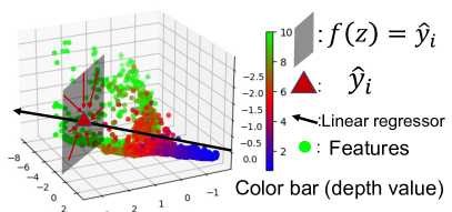
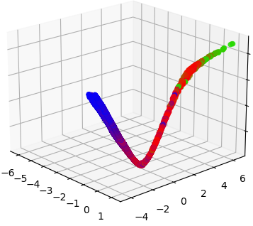
Encouraging the same intrinsic dimension. Figure 1(a) plots pixel-wise representations of the last hidden layer’s feature space, depicted as dots with different colors corresponding to ground truth depth. These representations are obtained from a batch of images from the NYU-v2 test set for depth estimation. A modified ResNet-50 produces these representations, with the last hidden layer changed to dimension 3 for visualization. This figure provides a visualization of the last hidden layer’s feature space, where the representations lay on a manifold where the ID varies locally from (blue region) to (green region). The black arrow represents the linear regressor’s weight vector , and the predicted depth is obtained by mapping (represented as dots) to . The gray plane represents the solution space of , and the entropy of its distribution in this plane, i.e. , can be seen as an approximate of .
The target space for depth estimation is one-dimensional; enforcing an intrinsic dimension to match the 1D target space will squeeze the feature space into a line. Under such a scenario, the solution space of is compressed into a point, implying (discrete case) and a lower . Lower for all implies a lower . Thus, by controlling the ID, we obtain a lower , implying a higher generalization ability. Since the ID of the feature space is commonly higher than the ID of the target space, the first connection generally encourages learning a lower ID feature space.
In classification, we tighten clusters for a lower , while in regression, lowering the ID achieves a lower . Lowering the ID of feature space can be intuitively understood as tightening the clusters in classification, where each solution space represents a cluster in classification.
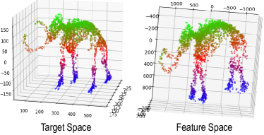
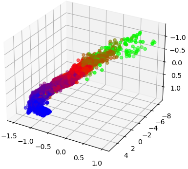
Enforcing topological similarity. Figure 1(b) provides a PCA visualization (from dimension to dimension, t-sne visualization can be found in Figure 3) of the feature space with a ’Mammoth’ shape target space (see Sec. 5.1 for details). This feature space is topologically similar to the target space, which indicates regression potentially captures the topology of the target space. The second connection suggests improving such similarity.
3.5 Encouraging the Same Intrinsic Dimension
Now, we can establish our first connection, which reveals that is bounded by the ID of the feature space. Note, intrinsic dimension is not a well-defined mathematical object, and different mathematical definitions exist (Ma et al., 2018; Birdal et al., 2021). We first define Intrinsic Dimension following Ghosh & Motani (2023):
Definition 1.
(Intrinsic Dimension). We define the intrinsic dimension of the manifold of a random variable as
| (4) |
where can be regard as the intrinsic dimension locally at point in the manifold . represent random random variables, means there exist continuous functions such that and . is a new random variable that follows distribution given by:
| (5) |
where .
Theorem 3.
Assume that lies in a manifold and the is a manifold corresponding to the distribution . Let be some function of :
| (6) |
where is the probability of when is uniformly distributed across , and is any point on . Then, as , we have:
| (7) | ||||
| (8) |
for some fixed scalar K. is the intrinsic dimension of the manifold .
Theorem 3 is derived from [(Ghosh & Motani, 2023), Proposition 1]. The detailed proof is provided in Appendix A.3. Theorem 3 states that the conditional entropy is bounded by the IDs of manifolds corresponding to the distribution , and the bound is tight when are uniformly distributed across the manifolds.
Since , Theorem 3 suggests that reducing the intrinsic dimension of the feature space will lead to a lower , which in turn implies a better generalization performance based on Theorem 2. On the other hand, the ID of should not be less than the intrinsic dimension of the target space to guarantee sufficient representation capabilities. Thus, a with an intrinsic dimension equal to the dimensionality of the target space is desirable.
3.6 Enforcing Topological Similarity
Below, we establish the second connection: topological similarity between the feature and target spaces. We first define the optimal representation following Achille & Soatto (2018b).
Definition 2.
(Optimal Representation). The representation is optimal if (1) and (2) is fully determined given , i.e. is minimal.
In Definition 2, means is sufficient for the target , while is minimal means discards all information that is not relevant to , and is fully determined given . For continuous entropy, a minimal implies that , as is distributed as a delta function once given . In the discrete case, .
Proposition 2.
Let the target where is fully determined by and is the aleatoric uncertainty that is independent of . Assume the underlying mapping between and and its inverse are continuous, where the continuous mapping is based on the topology induced by the Euclidean distance. Then the representation is optimal if and only if is homeomorphic to .
The detailed proof of Proposition 2 is provided in Appendix A.4. Proposition 2 demonstrates that the optimal is homeomorphic to , implying the need to learn a that is homeomorphic to . However, directly enforcing homeomorphism can be challenging to achieve since is generally unknown, and the representation typically lies in a high-dimensional space that cannot be modeled without sufficient data samples. As such, we opted to enforce the topological similarity between the target and feature spaces, preserving topological features similar to homomorphism. Here, topological similarity refers to the similarity in topological features, such as clusters and loops, and their localization (Trofimov et al., 2023). The two established connections imply that the desired should be topologically similar to the target space and share the same ID as the target space.
4 PH-Reg for Regression
Our analysis in Sec. 3 inspires us to learn a feature space that is (1) topologically similar to the target space and (2) with an intrinsic dimension (ID) equal to that of the target space. To this end, we propose a regularizer named Persistent Homology Regression Regularizer (PH-Reg). PH-Reg features two terms: an intrinsic dimension term and a topology term . follows Birdal’s regularizer (Birdal et al., 2021) to control the ID of feature space. Additionally, it considers the target space to ensure sufficient representation capabilities. exploit the topology autoencoder (Moor et al., 2020) to encourage the topological similarity. Note the two regularizer terms are mainly introduced to verify our connections, and other ID and topology regularizers can also be considered. However, empirical observations suggest that our and effectively align with our established connections, perform well, and do not conflict with each other.
We first introduce some notations. Let represent the set of samples from , and be the labels corresponding to . We denote the -dimensional persistent homology. Intuitively, can be regarded as a set of edge lengths, where the edges are derived from the minimum spanning tree obtained from the distance matrix of . We denote the set of the index of edges in the minimum spanning trees of and , respectively, and the corresponding length of the edges. Let be the sum of edge lengths of the minimum spanning trees corresponding to . We define similarly. Some topology preliminaries are given in Appendix D.
Birdal et al. (2021) suggests to estimate the intrinsic dimension as the slope between and . Note, the definition of intrinsic dimension used in Birdal et al. (2021) is based on the -dimensional persistent homology , which is different from ours (Definition 1, coming from Ghosh & Motani (2023)). However, both definitions define the same object, i.e. the intrinsic dimension, and it is thus reasonable to exploit Birdal et al. (2021)’s method to constrain the intrinsic dimension.
Let , where is the subset sampled from a batch, with size . Let for , and . Birdal et al. (2021) encourage a lower intrinsic dimension feature space by minimizing the slope between and , which can be estimated via the least square method:
| (9) |
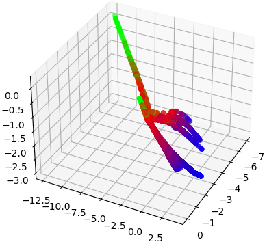
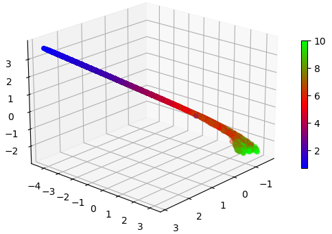
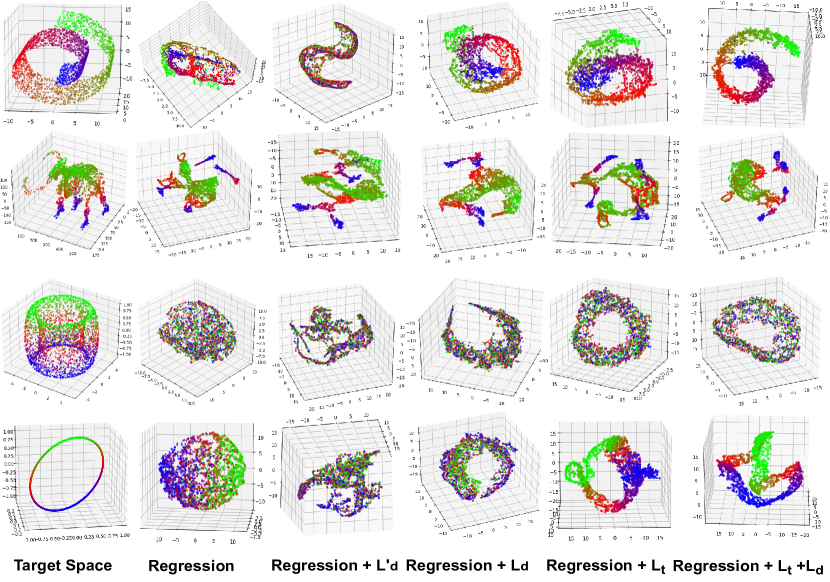
purely encourage the feature space to have a lower intrinsic dimension; sometimes it may even result in an intrinsic dimension lower than that of the target space (see Figure 3, Swiss Roll, where the target space is two-dimensional and the feature space is almost one-dimensional.). In contrast, we wish to lower the ID of the feature space while preventing it from lower than that of the target space. We propose to minimize slope between and :
| (10) |
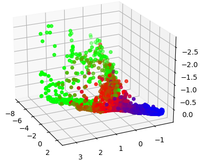
where . Compared with , further exploits the topological information of the target space through . When the feature and target spaces have the same ID, for all and is in its minimal. As shown in Figure 2(c) and Figure 3, well controls the ID of the feature space while better preserving the topology of the target space.
The topology autoencoder (Moor et al., 2020) enforces the topological similarity between the feature and the target spaces by preserving -dimensional topologically relevant distances from the two spaces. We exploit it as the topology part :
| (11) | ||||
| (12) |
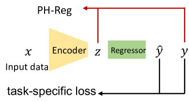
As shown in Figure 2(d) and Figure 3, well preserves the topology of the target space. We define the persistent homology regression regularizer, PH-Reg, as . As shown in Figure 2(e) and Figure 3, PH-Reg can both encourage a lower intrinsic dimension and preserve the topology of target space. The final loss function is defined as:
| (13) |
where is the task-specific regression loss and are trade-off parameters, and their values are determined by the value of the task task-specific loss , e.g. for a high , and should also be set to high values.
5 Experiments
We compare our method with four methods. 1) Information Dropout (InfDrop) (Achille & Soatto, 2018b). InfDrop serves as an IB baseline. It functions as a regularizer designed based on IB, aiming to learn representations that are minimal, sufficient, and disentangled. 2) Ordinal Entropy (OE) (Zhang et al., 2023). OE acts as a regression baseline. It takes the advantages of classification by learning higher entropy feature space for regression tasks. 3) Birdal’s regularizer (i.e., ) (Birdal et al., 2021) serves as an intrinsic dimension baseline. 4) Topology Autoencoder (i.e., ) (Moor et al., 2020) serves as a topology baseline. Note that the proposed PH-Reg is mainly introduced to verify the established connections, and we do not aim for the state-of-the-art results.
5.1 Coordinate Prediction on the Synthetic Dataset
To verify the topological relationship between the feature space and target space, we synthetic a dataset that contains points sampled from topologically different objects, including swiss roll, torus, circle and the more complex object “mammoth” (Coenen & Pearce, 2019). We randomly sample points with coordinate from each object. These points are then divided into sets of for training, for validation, and for testing. Each point is encoded into a dimensional vector , where the dimensions - are signal and the rest dimensions are noise. The coordinate prediction task aims to learn the mapping from to , and the mean-squared error is adopted as the evaluation metric. We use a two-layer fully connected neural network with 100 hidden units as the baseline architecture. More details are given in Appendix E.
| Method | Swiss Roll | Mammoth | Torus | Circle |
| Baseline | 2.99 0.43 | 211 55 | 3.01 0.11 | 0.154 0.006 |
| InfDrop | 4.15 0.37 | 367 50 | 2.05 0.04 | 0.093 0.003 |
| OE | 2.95 0.69 | 187 88 | 2.83 0.07 | 0.114 0.007 |
| 2.74 0.85 | 141 104 | 1.13 0.06 | 0.171 0.04 | |
| 0.66 0.08 | 89 66 | 0.62 0.12 | 0.090 0.019 | |
| 1.83 0.70 | 80 61 | 0.95 0.05 | 0.036 0.004 | |
| 0.61 0.17 | 49 27 | 0.61 0.05 | 0.013 0.008 |
Table 1 shows that encouraging a lower intrinsic dimension while considering the target space () enhances performance, particularly for Swiss Roll and Torus. In contrast, naively lowering the intrinsic dimension () performs poorly. Enforcing the topology similarity between the feature space and target space () decreases the by more than , except for the Swiss roll. The best gains, however, are achieved by incorporating both and , which decrease the even more than for the circle coordinate prediction task. Figure 3 shows feature space visualization results using t-SNE ( dimensions dimensions). The feature space of the regression baseline shows a similar structure to the target space, especially for Swiss roll and mammoth, which indicates regression potentially captures the topology of the target space. Regression significantly preserves the topology of the target space. Regression potentially preserves the topology of the target space, e.g. circle, while it primarily reduces the complexity of the feature space by maintaining the same intrinsic dimension as the target space. Combining both and in regression preserves the topology information while also reducing the complexity of the feature space, i.e. lower its intrinsic dimension.
5.2 Real-World Regression Tasks
We conduct experiments on three real-world regression tasks, including depth estimation (Table 2), super-resolution (Table 3) and age estimation (Table 4). The target spaces of the three tasks are topologically different, i.e. a - dimensional line for depth estimation, -dimensional space for super-resolution and discrete points for age estimation. Detailed settings, related introductions and more results are given in Appendix F.
Results on the three tasks demonstrate that both and can enhance performance, and combining both further boosts the performance. Specifically, combining both achieves overall improvements (i.e. ALL) on age estimation, a PSNR improvement of on super-resolution for Urban100, and a reduction of error on depth estimation.
| Method | ALL | Many | Med. | Few |
| Baseline | 7.80 0.12 | 6.80 0.06 | 9.11 0.31 | 13.63 0.43 |
| InfDrop | 8.04 0.14 | 7.14 0.20 | 9.10 0.71 | 13.61 0.32 |
| OE | 7.65 0.13 | 6.72 0.09 | 8.77 0.49 | 13.28 0.73 |
| 7.75 0.05 | 6.80 0.11 | 8.87 0.05 | 13.61 0.50 | |
| 7.64 0.07 | 6.82 0.07 | 8.62 0.20 | 12.79 0.65 | |
| 7.50 0.04 | 6.59 0.03 | 8.75 0.03 | 12.67 0.24 | |
| 7.32 0.09 | 6.50 0.15 | 8.38 0.11 | 12.18 0.38 |
| Method | Set5 | Set14 | B100 | Urban100 | DIV2K |
| Baseline | 32.241 | 28.614 | 27.598 | 26.083 | 28.997 |
| InfDrop | 32.219 | 28.626 | 27.594 | 26.059 | 28.980 |
| OE | 32.280 | 28.659 | 27.614 | 26.117 | 29.005 |
| 32.252 | 28.625 | 27.599 | 26.078 | 28.989 | |
| 32.293 | 28.644 | 27.619 | 26.151 | 29.022 | |
| 32.322 | 28.673 | 27.624 | 26.169 | 29.031 | |
| 32.288 | 28.686 | 27.627 | 26.179 | 29.038 |
| Method | REL | RMS | ||||
| Baseline | 0.792 | 0.955 | 0.990 | 0.153 | 0.512 | 0.064 |
| InfDrop | 0.791 | 0.960 | 0.992 | 0.153 | 0.507 | 0.064 |
| OE | 0.811 | - | - | 0.143 | 0.478 | 0.060 |
| 0.804 | 0.954 | 0.988 | 0.151 | 0.502 | 0.063 | |
| 0.795 | 0.959 | 0.992 | 0.150 | 0.497 | 0.063 | |
| 0.798 | 0.958 | 0.990 | 0.149 | 0.502 | 0.063 | |
| 0.807 | 0.959 | 0.992 | 0.144 | 0.481 | 0.061 |
5.3 Ablation Studies
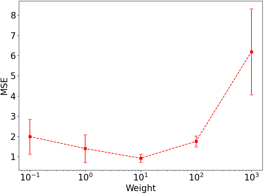
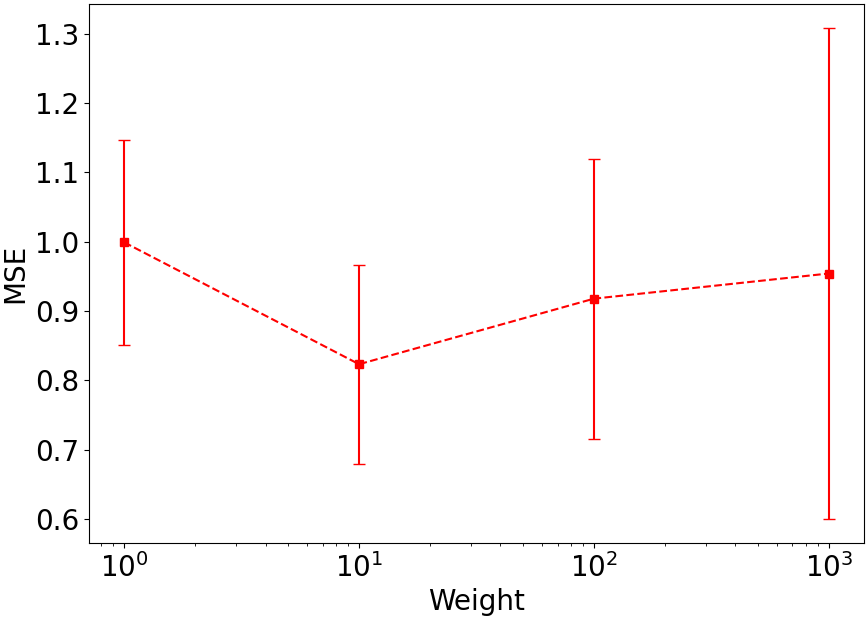
Hyperparameter and : We maintain and at their default value for Swiss roll coordinate prediction, and we vary one of them to examine their impact. Figure 4(a) shows when , the MSE decreases consistently as increases. However, it tends to overtake the original learning objective when set too high, i.e. . Regarding the , as shown in Figure 4(b), MSE remains relatively stable over a large range of , with a slight increase in variance when .
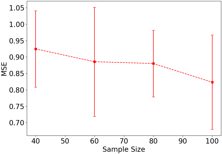
Sample Size (): In practice, we model the feature space using a limited number of samples within a batch. For dense prediction tasks, the available No. of samples is very large (No. pixels per image batch size), while it is constrained to the batch size for image-wise prediction tasks. We investigate the influence of from Eq. 10 and 11 on Swiss roll coordinate prediction. Figure 4(c) shows our PH-Reg performs better with a larger , while maintaining stability even with a small .
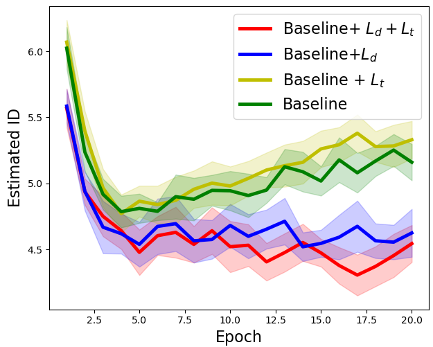
ID of different methods: Figure 4(d) displays the intrinsic dimension of the last hidden layer, estimated using TwoNN (Facco et al., 2017), for the testing set of NYU-Depth-v2 from different methods throughout training. While our method is based on the Birdal’s estimator (Birdal et al., 2021), another estimator, TwoNN, captures a decrease in intrinsic dimension when applied . We observe that without , the intrinsic dimension tends to increase after epoch , potentially overfitting details, whereas prevents such a trend.
Efficiency: Efficiency-wise, the computing complexity equals finding the minimum spanning tree from the distance matrix of the samples, which have a complexity of using the simple Kruskal’s Algorithm, and it can speed up with some advanced methods (Bauer, 2021). The synthetic experiments (Table 5) use a simple 2-layer MLP, so the regularizer adds significant computing time. However, the real-world experiments on depth estimation (Table 5) use a ResNet-50 backbone, and the added time and memory are negligible (18.6% and 0.3%, respectively), even with . These increases are only during training and do not add demands for inference.
| Regularizer | Coordinate Prediction | Depth Estimation | |||
| ( Layer MLP) | (ResNet-50) | ||||
| Training(s) | Memory (MB) | Training(s) | Memory (MB) | ||
| 0 | - | 8.88 | 959 | 1929 | 11821 |
| 100 | 175.06 | 959 | 1942 | 11833 | |
| 100 | 439.68 | 973 | 1950 | 12211 | |
| 100 | 617.41 | 973 | 1980 | 12211 | |
| 300 | - | - | 2370 | 12211 | |
6 Conclusion
In this paper, we establish novel connections between topology and the IB principle for regression representation learning. The established connections imply that the desired should exhibit topological similarity to the target space and share the same intrinsic dimension as the target space. Inspired by the connections, we proposed a regularizer to learn the desired . Experiments on synthetic and real-world regression tasks demonstrate its benefits.
7 Impact Statements
This paper presents work whose goal is to advance the field of Machine Learning. There are many potential societal consequences of our work, none which we feel must be specifically highlighted here.
References
- Achille & Soatto (2018a) Achille, A. and Soatto, S. Emergence of invariance and disentanglement in deep representations. The Journal of Machine Learning Research, 19(1):1947–1980, 2018a.
- Achille & Soatto (2018b) Achille, A. and Soatto, S. Information dropout: Learning optimal representations through noisy computation. IEEE transactions on pattern analysis and machine intelligence, 40(12):2897–2905, 2018b.
- Ansuini et al. (2019) Ansuini, A., Laio, A., Macke, J. H., and Zoccolan, D. Intrinsic dimension of data representations in deep neural networks. Advances in Neural Information Processing Systems, 32, 2019.
- Barannikov et al. (2021a) Barannikov, S., Trofimov, I., Balabin, N., and Burnaev, E. Representation topology divergence: A method for comparing neural network representations. ICML, 2021a.
- Barannikov et al. (2021b) Barannikov, S., Trofimov, I., Sotnikov, G., Trimbach, E., Korotin, A., Filippov, A., and Burnaev, E. Manifold topology divergence: a framework for comparing data manifolds. NeurIPS, 34:7294–7305, 2021b.
- Bauer (2021) Bauer, U. Ripser: efficient computation of vietoris–rips persistence barcodes. Journal of Applied and Computational Topology, 5(3):391–423, 2021.
- Bengio et al. (2013) Bengio, Y., Courville, A., and Vincent, P. Representation learning: A review and new perspectives. IEEE transactions on pattern analysis and machine intelligence, 35(8):1798–1828, 2013.
- Bevilacqua et al. (2012) Bevilacqua, M., Roumy, A., Guillemot, C., and Alberi-Morel, M. L. Low-complexity single-image super-resolution based on nonnegative neighbor embedding. 2012.
- Birdal et al. (2021) Birdal, T., Lou, A., Guibas, L. J., and Simsekli, U. Intrinsic dimension, persistent homology and generalization in neural networks. Advances in Neural Information Processing Systems, 34:6776–6789, 2021.
- Boudiaf et al. (2020) Boudiaf, M., Rony, J., Ziko, I. M., Granger, E., Pedersoli, M., Piantanida, P., and Ayed, I. B. A unifying mutual information view of metric learning: cross-entropy vs. pairwise losses. In European conference on computer vision, pp. 548–564. Springer, 2020.
- Brown et al. (2022a) Brown, B. C., Caterini, A. L., Ross, B. L., Cresswell, J. C., and Loaiza-Ganem, G. Verifying the union of manifolds hypothesis for image data. In The Eleventh International Conference on Learning Representations, 2022a.
- Brown et al. (2022b) Brown, B. C., Juravsky, J., Caterini, A. L., and Loaiza-Ganem, G. Relating regularization and generalization through the intrinsic dimension of activations. arXiv preprint arXiv:2211.13239, 2022b.
- Chazal & Michel (2021) Chazal, F. and Michel, B. An introduction to topological data analysis: fundamental and practical aspects for data scientists. Frontiers in artificial intelligence, 4:108, 2021.
- Chen et al. (2019) Chen, C., Ni, X., Bai, Q., and Wang, Y. A topological regularizer for classifiers via persistent homology. In The 22nd International Conference on Artificial Intelligence and Statistics, pp. 2573–2582. PMLR, 2019.
- Coenen & Pearce (2019) Coenen, A. and Pearce, A. Understanding umap, mammoth dataset, 2019. URL https://github.com/MNoichl/UMAP-examples-mammoth-/tree/master.
- Eigen et al. (2014) Eigen, D., Puhrsch, C., and Fergus, R. Depth map prediction from a single image using a multi-scale deep network. Advances in neural information processing systems, 27, 2014.
- Facco et al. (2017) Facco, E., d’Errico, M., Rodriguez, A., and Laio, A. Estimating the intrinsic dimension of datasets by a minimal neighborhood information. Scientific reports, 7(1):12140, 2017.
- Ghosh & Motani (2023) Ghosh, R. and Motani, M. Local intrinsic dimensional entropy. AAAI, 2023.
- Hatcher (2001) Hatcher, A. Algebraic topology. Cambridge University Press, 2001.
- He et al. (2016) He, K., Zhang, X., Ren, S., and Sun, J. Deep residual learning for image recognition. In Proceedings of the IEEE conference on computer vision and pattern recognition, pp. 770–778, 2016.
- Hofer et al. (2019) Hofer, C., Kwitt, R., Niethammer, M., and Dixit, M. Connectivity-optimized representation learning via persistent homology. In International conference on machine learning, pp. 2751–2760. PMLR, 2019.
- Huang et al. (2015) Huang, J.-B., Singh, A., and Ahuja, N. Single image super-resolution from transformed self-exemplars. In Proceedings of the IEEE conference on computer vision and pattern recognition, pp. 5197–5206, 2015.
- Kawaguchi et al. (2023) Kawaguchi, K., Deng, Z., Ji, X., and Huang, J. How does information bottleneck help deep learning? ICML, 2023.
- Lee et al. (2019) Lee, J. H., Han, M.-K., Ko, D. W., and Suh, I. H. From big to small: Multi-scale local planar guidance for monocular depth estimation. arXiv preprint arXiv:1907.10326, 2019.
- Lim et al. (2017) Lim, B., Son, S., Kim, H., Nah, S., and Mu Lee, K. Enhanced deep residual networks for single image super-resolution. In Proceedings of the IEEE conference on computer vision and pattern recognition workshops, pp. 136–144, 2017.
- Ma et al. (2018) Ma, X., Wang, Y., Houle, M. E., Zhou, S., Erfani, S., Xia, S., Wijewickrema, S., and Bailey, J. Dimensionality-driven learning with noisy labels. In International Conference on Machine Learning, pp. 3355–3364. PMLR, 2018.
- Martin et al. (2001) Martin, D., Fowlkes, C., Tal, D., and Malik, J. A database of human segmented natural images and its application to evaluating segmentation algorithms and measuring ecological statistics. In Proceedings Eighth IEEE International Conference on Computer Vision. ICCV 2001, volume 2, pp. 416–423. IEEE, 2001.
- Moor et al. (2020) Moor, M., Horn, M., Rieck, B., and Borgwardt, K. Topological autoencoders. In International conference on machine learning, pp. 7045–7054. PMLR, 2020.
- Rieck et al. (2020) Rieck, B., Yates, T., Bock, C., Borgwardt, K., Wolf, G., Turk-Browne, N., and Krishnaswamy, S. Uncovering the topology of time-varying fmri data using cubical persistence. Advances in neural information processing systems, 33:6900–6912, 2020.
- Shwartz-Ziv & Tishby (2017) Shwartz-Ziv, R. and Tishby, N. Opening the black box of deep neural networks via information. arXiv preprint arXiv:1703.00810, 2017.
- Silberman et al. (2012) Silberman, N., Hoiem, D., Kohli, P., and Fergus, R. Indoor segmentation and support inference from rgbd images. In European conference on computer vision, pp. 746–760. Springer, 2012.
- Timofte et al. (2017) Timofte, R., Agustsson, E., Van Gool, L., Yang, M.-H., and Zhang, L. Ntire 2017 challenge on single image super-resolution: Methods and results. In Proceedings of the IEEE conference on computer vision and pattern recognition workshops, pp. 114–125, 2017.
- Tishby & Zaslavsky (2015) Tishby, N. and Zaslavsky, N. Deep learning and the information bottleneck principle. In 2015 ieee information theory workshop (itw), pp. 1–5. IEEE, 2015.
- Trofimov et al. (2023) Trofimov, I., Cherniavskii, D., Tulchinskii, E., Balabin, N., Burnaev, E., and Barannikov, S. Learning topology-preserving data representations. ICLR, 2023.
- Tulchinskii et al. (2023) Tulchinskii, E., Kuznetsov, K., Kushnareva, L., Cherniavskii, D., Barannikov, S., Piontkovskaya, I., Nikolenko, S., and Burnaev, E. Intrinsic dimension estimation for robust detection of ai-generated texts. NeurIPS, 2023.
- Yang et al. (2021) Yang, Y., Zha, K., Chen, Y., Wang, H., and Katabi, D. Delving into deep imbalanced regression. In International Conference on Machine Learning, pp. 11842–11851. PMLR, 2021.
- Zeyde et al. (2012) Zeyde, R., Elad, M., and Protter, M. On single image scale-up using sparse-representations. In Curves and Surfaces: 7th International Conference, Avignon, France, June 24-30, 2010, Revised Selected Papers 7, pp. 711–730. Springer, 2012.
- Zhang et al. (2023) Zhang, S., Yang, L., Mi, M. B., Zheng, X., and Yao, A. Improving deep regression with ordinal entropy. ICLR, 2023.
- Zhu et al. (2018) Zhu, W., Qiu, Q., Huang, J., Calderbank, R., Sapiro, G., and Daubechies, I. Ldmnet: Low dimensional manifold regularized neural networks. In Proceedings of the IEEE conference on computer vision and pattern recognition, pp. 2743–2751, 2018.
Appendix A Proofs
A.1 Proof of the Theorem 1
Theorem 1 Assume that the conditional entropy is a fixed constant for for some set of the random variables, or is determined given . Then, .
Proof.
From the definition of the mutual information, we have
By substituting the right-hand side of this equation into ,
| (14) |
Since ,
| (15) | ||||
| (16) |
1) If is a constant for . Since is a fixed constant for any , this implies that
where is a fixed constant for . Thus:
2) If is determined given , then is not a term can be optimized. Since is a fixed constant for any :
A.2 Proof of the Theorem 2 and Proposition 1
Theorem 2 Consider dataset sampled from distribution , where is the input, is the corresponding representation, and is the label. Let be the maximum distance of to its nearset . Assume follows a distribution and the dispersion of is bounded by its entropy:
| (17) |
where is the mean of the distribution and is some function of . Assume the regressor f is -Lipschitz continuous, then as , we have:
| (18) |
Proof.
For any sample , we define its local neighborhood set as
| (19) |
For each set , we have
| (20) | ||||
| (21) | ||||
| (22) | ||||
| (23) | ||||
| (24) | ||||
| (25) |
We denote the probability distribution over as , where . Then, we have
| (26) | ||||
| (27) | ||||
| (28) |
As , we can approximate as . Since , we have for all , and can thus be approximate as . We have:
| (29) | |||
| (30) | |||
| (31) | |||
| (32) | |||
| (33) |
Proposition 1 If is a multivariate normal distribution , where is a scalar and is the mean of the distribution . Then, the function in Theorem 2 can be selected as , where is the dimension of . If is a uniform distribution, then the can be selected as .
Proof.
We first consider the case when . Assume , then :
| (34) | ||||
| (35) | ||||
| (36) | ||||
| (37) | ||||
| (38) | ||||
| (39) | ||||
| (40) | ||||
| (41) | ||||
| (42) | ||||
| (43) | ||||
| (44) |
We have the following:
| (45) |
The following also holds:
| (46) |
Thus, we have:
| (47) |
Similarly, if is a uniform distribution , then its variance is given by:
| (49) |
and its entropy is given by:
| (50) |
We have:
| (51) |
Finally,
| (52) |
Thus, in Theorem 2 can be selected as , when is a uniform distribution
A.3 Proof of the Theorem 3
We first show a straightforward result of [(Ghosh & Motani, 2023), Proposition 1]:
Lemma 1.
Assume that lies in a manifold and the is a manifold corresponding to the distribution . Assume for all features , the following holds:
| (53) |
where is some function of . The above imposes a constraint where the distribution is uniformly distributed across . Then, as , we have:
| (54) |
for some fixed scalar K. is the intrinsic dimension of the manifold .
Proof.
By using the same proof technique as [(Ghosh & Motani, 2023), Proposition 1], we can show
| (55) |
Since , the result follows.
Theorem 3 Assume that lies in a manifold and the is a manifold corresponding to the distribution . Let be some function of :
| (56) |
where is the probability of when is uniformly distributed across , and is any point on . Then, as , we have:
| (57) |
for some fixed scalar K. is the intrinsic dimension of the manifold .
Proof.
Since the uniform distribution has the largest entropy over all distributions over the support , based on Lemma 1, we thus have:
| (58) |
A.4 Proof of the Proposition 2
Proposition 2 Let the target where is fully determined by and is the aleatoric uncertainty that is independent of . Assume the underlying mapping between and and its inverse are continuous, where the continuous mapping is based on the topology induced by the Euclidean distance. Then the representation is optimal if and only if is homeomorphic to .
Proof.
If is optimal (optimal is homeomorphic to ):
| (59) |
| (60) |
Since is optimal, we have . Based on the two equations above, we have:
| (61) |
Since is fully determined by and , is also fully determined by . Thus, for each , there exists and only exists one corresponding to the , and thus the mapping function exists.
is optimal also means is fully determined given , Since is independent of :
| (62) |
thus, for each , there exist and only exist one corresponding to the . Thus, the mapping function is a bijection, and since and are continuous, is homeomorphic to .
If is homeomorphic to : ( is homeomorphic to optimal ):
is homeomorphic to means a continuous bijection exist between and , thus and is minimal. We have:
| (63) |
thus, is optimal.
Appendix B Discussions about Theorem 1
Choice of in Theorem 1: in means we need to maximize for sufficiency, while we want to minimize for minimality. When , then we value the minimality more than the sufficiency, resulting in the need to maximize . But, in the typical setting, we always value more than for a good task-specific performance, and will lead compressed to be a single point, as is minimal and is maximized in this case. The qualitative behavior should change based on or , as it controls which we value the more: sufficiency or minimality.
Difference between the target and the predicted : The target is different from the predicted . always equals to if we exploit neural networks as deterministic functions. In an extreme case, we can treat the predicted as the representation , which shows minimizing is the learning target. From the invariance representation learning point of view, lowering is learning invariance representations with respect to .
More discussions about the assumptions: For discrete entropy, is determined given implies is a constant for , as here. However, this does not hold for differential entropy. For differential entropy, is determined given means , since given Y, Z is distributed as a delta function in this case.
Appendix C Connections with the bound in Kawaguchi et al. (2023)
Kawaguchi et al. (2023) provide several bounds that are all applicable for both classification and regression for various cases. In the case where the encoder model (whose output is ) and the training dataset of the downstream task are dependent (e.g., this is when for is dependent of all training data points through the training of by using ), they show that any valid and general generalization bound of the information bottleneck must include two terms, and , where the second term measures the effect of overfitting the encoder . This is because the encoder can compress all information to minimize arbitrarily well while overfitting to the training data: e.g., we can simply set for all and for all for some constant to achieve the best training loss while minimizing and performing arbitrarily poorly for test loss. Given this observation, they prove the first rigorous generalization bounds for two separate cases based on the dependence of and . Their generalization bounds scales with without the second term in case of and being independent, and with and in case of and being dependent.
In Theorem 2, we consider the case where and are independent, since in is drawn without dependence on the entire data points in equation (18). Thus, our results are consistent and do not contradict with previous findings. Unlike the previous bounds, our bound is determined by the function , which characterizes the dispersion or the standard deviation of a distribution by its entropy. The function exists for general cases, as the dispersion or the standard deviation and the entropy commonly can be estimated for a specific distribution. We thus can find a function to upper bound the relationship on the entropy and its dispersion or the standard deviation.
It is worth mentioning that we are not targeting a tight or an advanced bound here. Our bound is introduced to support the analysis that follows after Theorem 2, which is challenging with the previous bounds.
Appendix D Preliminaries on Topology
The simplicial complex is a central object in topological data analysis, and it can be exploited as a tool to model the ‘shape’ of data. Given a set of finite samples , the simplicial complex can be seen as a collection of simplices of varying dimensions: vertices , edges, and the higher-dimensional counterparts. The faces of a simplex is the simplex spanned by the subset of . The dimension of the simplicial complex is the largest dimension of its simplices. A simplicial complex can be regarded as a high-dimensional generalization of a graph, and a graph can be seen as a 1-dimensional simplicial complex. For each , there exist many ways to build simplicial complexes and the Vietoris-Rips Complexes are widely used:
Definition 3.
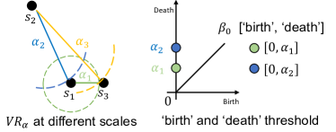
(Vietoris-Rips Complexes). Given a set of finite samples sampled from the feature space or target space and a threshold , the Vietoris-Rips Complexes VRα is defined as:
| (64) |
where is the Euclidean distance between samples and .
is the set of all simplicial complexes where the pairwise distance is within the threshold . Let denote the vector space generated by its -dimensional simplices over 222It is not specific to , but is a typical choice.. The boundary operator maps each simplex to its boundary , which consists of the sum of all its faces, is a homomorphism from to . It can be shown that , which leads to the chain complex: , and the homology group is defined as the quotient group . ker represents kernel, which is the set of all elements that are mapped to the zero element. im represents image, which is the set of all the outputs. Rank is known as the Betti number , which counts the number of -dimensional holes and can be used to represent the topological features of the manifold that the set of points sampled from.
However, the is obtained based on a single , which is easily affected by small changes in . Thus it is not robust and is of limited use for real-world datasets. The persistent homology considers all the possible instead of a single one, which results in a sequence of . This is achieved through a nested sequence of simplicial complexes, called filtration: for . Let be the interval corresponding to a -dimensional hole ‘birth’ at the threshold and ‘death’ at the threshold , we denote the set of ‘birth’ and ‘death’ intervals of the -dimensional holes. We only exploit in our PH-Reg, since we exploit the topological autoencoder as the topology part and higher topological features merely increase its runtime. An illustration of the calculation is given in Figure 5(b). We define , where is the length of the interval .
Appendix E More details about the Coordinate Prediction task
Details about the synthetic dataset: We encode coordinates into dimensional vectors , where the dimensions are signal and the rest dimensions are noise. The encoder functions are defined as:
-
•
-
•
-
•
-
•
As shown above, the accurate coordinates can be obtained correctly when are given. We introduce noise to the remaining dimensions by using on other randomly selected samples . The proximity of to can be intuitively seen as an indicator of the noise’s relationship to the signal.
More training details: We train the models for epochs using AdamW as the optimizer with a learning rate of . We report results as mean standard variance over runs. For the regression baseline Oridnal Entropy and the IB baseline Information Dropout, we tried various weights and reported the best results. The trade-off parameters and are default set to and , respectively, while is set to and is set to for Mammoth, and is set to 1 for torus and circle.
Appendix F Details about the real-world tasks
F.1 Age estimation on AgeDB-DIR dataset
We exploit the AgeDB-DIR (Yang et al., 2021) for age estimation task. We follow the setting of Yang et al. (2021) and exploit their regression baseline model, which uses ResNet-50 (He et al., 2016) as the backbone. The evaluation metrics are MAE and geometric mean(GM), and the results are reported on the whole set and the three disjoint subsets, i.e. Many, Med. and Few. The trade-off parameters and are set to and , respectively. Table 6 shows that both and can improve the performance, and combining both achieves overall improvements (i.e. ALL) on MAE and overall improvements on GM.
| Method | MAE | GM | ||||||
| ALL | Many | Med. | Few | ALL | Many | Med. | Few | |
| Baseline (Yang et al., 2021) | 7.80 0.12 | 6.80 0.06 | 9.11 0.31 | 13.63 0.43 | 4.98 0.05 | 4.32 0.06 | 6.19 0.07 | 10.29 0.57 |
| Information dropout (Achille & Soatto, 2018b) | 8.04 0.14 | 7.14 0.20 | 9.10 0.71 | 13.61 0.32 | 5.11 0.06 | 4.49 0.17 | 6.14 0.49 | 10.54 0.65 |
| Oridnal Entropy (Zhang et al., 2023) | 7.65 0.13 | 6.72 0.09 | 8.77 0.49 | 13.28 0.73 | 4.91 0.14 | 4.29 0.06 | 6.04 0.51 | 10.09 0.62 |
| 7.75 0.05 | 6.80 0.11 | 8.87 0.05 | 13.61 0.50 | 4.96 0.04 | 4.33 0.09 | 6.05 0.36 | 10.43 0.40 | |
| 7.64 0.07 | 6.82 0.07 | 8.62 0.20 | 12.79 0.65 | 4.85 0.05 | 4.27 0.06 | 5.91 0.13 | 9.75 0.53 | |
| 7.50 0.04 | 6.59 0.03 | 8.75 0.03 | 12.67 0.24 | 4.77 0.07 | 4.27 0.06 | 6.09 0.03 | 9.34 0.70 | |
| 7.32 0.09 | 6.50 0.15 | 8.38 0.11 | 12.18 0.38 | 4.69 0.07 | 4.15 0.08 | 5.64 0.09 | 8.99 0.38 | |
F.2 Super-resolutuion on DIV2K dataset
We exploit the DIV2K dataset (Timofte et al., 2017) for 4x super-resolution training (without the 2x pretrained model) and we evaluate on the validation set of DIV2K and the standard benchmarks: Set5 (Bevilacqua et al., 2012), Set14 (Zeyde et al., 2012), BSD100 (Martin et al., 2001), Urban100 (Huang et al., 2015). We follow the setting of Lim et al. (2017) and exploit their small-size EDSR model as our baseline architecture. We adopt the standard metric PNSR and SSIM. The trade-off parameters and are set to and , respectively. Table 3 shows that both and contribute to improving the baseline and adding both terms has the largest impact.
| Method | Set5 | Set14 | B100 | Urban100 | DIV2K |
| Baseline (Lim et al., 2017) | 32.241/ 0.8656 | 28.614/ 0.7445 | 27.598/ 0.7120 | 26.083/ 0.7645 | 28.997/ 0.8189 |
| Information dropout (Achille & Soatto, 2018b) | 32.219/ 0.8649 | 28.626/ 0.7441 | 27.594/ 0.7113 | 26.059/ 0.7624 | 28.980/ 0.8182 |
| Oridnal Entropy (Zhang et al., 2023) | 32.280/ 0.8653 | 28.659/ 0.7445 | 27.614/ 0.7119 | 26.117/ 0.7641 | 29.005/ 0.8188 |
| 32.252/ 0.8653 | 28.625/ 0.7443 | 27.599/ 0.7118 | 26.078/ 0.7638 | 28.989/ 0.8186 | |
| 32.293/ 0.8660 | 28.644/ 0.7453 | 27.619/ 0.7127 | 26.151/ 0.7662 | 29.022/0.8197 | |
| 32.322/ 0.8663 | 28.673/ 0.7455 | 27.624/ 0.7127 | 26.169/ 0.7665 | 29.031/ 0.8196 | |
| 32.288/ 0.8663 | 28.686/ 0.7462 | 27.627/ 0.7132 | 26.179/ 0.7670 | 29.038/ 0.8201 |
F.3 Depth estimation on NYU-Depth-v2 dataset
We exploit the NYU-Depth-v2 (Silberman et al., 2012) for the depth estimation task. We follow the setting of Lee et al. (2019) and use ResNet50 as our baseline architecture. We exploit the standard metrics of threshold accuracy , average relative error (REL), root mean squared error (RMS) and average error. The trade-off parameters and are both set to . Table 4 shows that exploiting and results in reduction of and in the and errors, respectively.