The complete exterior spacetime of spherical Brans-Dicke stars

Abstract

We derive the complete expression for the Brans Class I exterior spacetime explicitly in terms of the energy and pressures profiles of a stationary spherisymmetric gravity source. This novel and generic expression is achieved in a parsimonious manner, requiring only a subset of the Brans-Dicke field equation and the scalar equation. For distant orbiting test particles, this expression promptly provides a simple, closed and exact formula of the γ Eddington parameter, which reads $\gamma_{\,\text{exact}}=\frac{\omega+1+\left(\omega+2\right)\Theta}{\omega+2+\left(\omega+1\right)\Theta}$, where $\Theta$ is the ratio of the star’s “total pressure” integral over its energy integral. This non-perturbative result reproduces the usual Post-Newtonian $\frac{\omega+1}{\omega+2}$ expression in the case of a “Newtonian star”, in which the pressure is negligible with respect to the energy density. Furthermore, it converges to the General Relativity value ($\gamma_{\,\text{GR}}=1$) as the star’s equation of state approaches that of ultra-relativistic matter (in which case $\Theta$ approaches 1), a behavior consistent with broader studies on scalar-tensor gravity. Our derivation underscores the essence of these results involving (1) the key relevant portion of the Brans-Dicke field equations, (2) the uniqueness of the Brans Class I vacuum solution for the non-phantom action, viz. $\omega>-3/2$, and (3) the involvement of only two free parameters in this solution. From a practical standpoint, it elucidates how a given stellar interior structure model determines the star’s exterior gravitational field and impacts the motions of light objects (such as planets and accretion disks) orbiting it.

General Relativity (GR) proved to be a very powerful gravity theory, able to account for many physical and astrophysical issues. This includes Solar System dynamics [1, 2], binary pulsars dynamics [1, 3], daily Global Positioning System (GPS) technological application [4, 5], dynamics [6, 7, 8, 9] and optical effects (shadow) [10, 11, 12] in supermassive black holes’ neighborhood, and the ability of GR to account for many high energy astrophysics phenomena, like quasar or active galactic nuclei physics [13] and binary black holes merging [14]. Despite these many successes, the quest to quantize gravity and unify it with other known interactions has spurred significant efforts, which produce, such as via superstring theories, (classical) gravity theory in the low energy regime that qualitatively depart from GR by the presence of a scalar partner to the metric field. More specifically, the gravitational sector often achieves a Brans-Dicke (BD) structure [15, 16, 17], the BD theory being a special case of scalar-tensor (ST) theories [18, 19, 20]. In brief, while the metric of an ST theory describes the spacetime geometry in a GR similar way, the scalar field determines the local value of Newton’s gravitational “constant”, which then depends on the spatial location and varies with time. These theoretical circumstances have stimulated a significant revival of interest in ST theories in the past three decades, despite the aforementioned successes of GR. (See for instance [21, 22, 23] for overviews on BD/ST theories and their links with attempts to quantify gravity.) Hence, we revisit some aspects of BD gravity in this letter.

In far field regions, the ST nature of gravity leaves its imprint on the Eddington parameters $\left(\beta,\,\gamma\right)$, which determine the first Post-Newtonian (PN) terms of the metric in the PN approximation. On the other hand, the description of the strong field region is generally by far more complex. The Eddington parameters are defined in such a way that their GR values are $\left(\beta_{\,\text{GR}},\,\gamma_{\,\text{GR}}\right)=\left(1,1\right)$. Therefore, the closer to unity are $\left(\beta,\,\gamma\right)$ for a specific theory, the closer is the (far) metric from the GR one, and are the predicted particle’s orbit to GR’s predictions. Each of the ST theories previously specified is characterized by a specific $\omega\left(\Phi\right)$ function. The ST Eddington parameters reads [1]

$$\left\{\begin{array}[]{l}\beta=1+\frac{\Phi_{0}\omega_{0}^{\prime}}{\left(2\omega_{0}+3\right)\left(2\omega_{0}+4\right)^{2}}\\ \gamma=\frac{\omega_{0}+1}{\omega_{0}+2}\end{array}\right.$$ (1)

where $\omega_{0}=\omega\left(\Phi_{0}\right)$ and $\omega_{0}^{\prime}=\omega^{\prime}\left(\Phi_{0}\right)$, $\Phi_{0}$ being the value of the scalar at the considered event. The experimental tests constrain $\left(1-\gamma\right)$ at the $10^{-5}$ level (see chapter 7 of Ref. [2]), and require acceptable ST theories to satisfy $\omega_{0}>4\times 10^{-5}$. (Let us remind that the $\omega_{0}<-3/2$ values correspond to a “phantom” kinetic energy for the scalar field, a case that could be deemed unphysical. Accordingly, the $\omega_{0}\ll-1$ possibility is usually discarded.) If gravity would be of ST nature, it could seem unnatural that it is adjusted in such a way that it mimics so closely GR. However, it has been shown in the nineties that a significant subset of ST theories obey an “attractor mechanism” in which the Universe’s expansion drives the scalar field to a value for which $\omega\left(\Phi\right)$ diverges, which finally imposes the theory to mimic GR [24, 25].

The BD theory [15] corresponds to the case where $\omega$ is $\Phi$ independent, i.e. is constant. The theory offers the advantage that the exact and general vacuum static spherical solution can be written in explicit form. It is the Brans Class I solution in the $\omega>-3/2$ case. This solution, which depends on two parameters, is the BD counterpart of the GR Schwarzschild solution, which depends on just one parameter. However, there is a strong difference between BD and GR: the Birkhoff theorem no longer applies in BD gravity. Therefore, the Brans Class I solution only describes the external gravitational field of static spherical stars.

Gluing Brans Class I to a Newtonian star (a weak field star in which the pressure $p$ is negligible with respect to the energy density $\epsilon$) and Taylor expanding the exterior metric, Brans and Dicke essentially found

$$\left\{\begin{array}[]{l}\beta_{\,\text{BD}}=1\\ \gamma_{\,\text{BD}}=\frac{\omega+1}{\omega+2}\end{array}\right.$$ (2)

in their seminal paper [15], in accordance with (1). However, considering asymptotically flat solutions, the Taylor expansion of the metric, in its form involving the Eddington parameters, is generic in far regions of the spacetime. It is then also relevant in the case of a compact and static spherical star. The purpose of this letter is to provide the exact and readily applicable expressions of the Brans Class I solution parameters, and of the induced expression of $\gamma$, in terms of the stellar internal structure.

The (Jordan-frame) BD field equations read

$$R_{ab}-\frac{\omega}{\Phi^{2}}\partial_{a}\Phi\partial_{b}\Phi-\frac{1}{\Phi}\partial_{a}\partial_{b}\Phi+\Gamma_{ab}^{c}\partial_{c}\ln\Phi =\frac{8\pi}{\Phi}\left(T_{ab}-\frac{\omega+1}{2\omega+3}Tg_{ab}\right)$$ (3)

$$\partial_{a}\left(\sqrt{-g}g^{ab}\partial_{b}\Phi\right) =\frac{8\pi}{2\omega+3}T\sqrt{-g}.$$ (4)

Let us consider a static spherisymmetric spacetime in isotropic coordinates

$$ds^{2}=-A\left(r\right)dt^{2}+B\left(r\right)\left[dr^{2}+r^{2}\left(d\theta^{2}+\sin^{2}\theta d\varphi^{2}\right)\right]$$ (5)

with a scalar $\Phi\left(r\right)$. The stationarity and spherisymmetry also imposes the stress tensor to have the form (let us spot that stationarity prevents the existence of radial heat fluxes)

$$\left(T_{a}^{b}\right) =\text{diag}\bigl{(}-\epsilon,p_{\|},p_{\bot},p_{\bot}\bigr{)}$$ (6)

where $\bigl{(}\,\epsilon,p_{\|},p_{\bot}\bigr{)}$ are three $r$–dependent functions. Thence, the most general gravity source differs from the perfect fluid by the only anisotropy between the radial and orthogonal pressures $p_{\|}$ and $p_{\bot}$. The (3)–(4) system yields four independent non-trivial equations. These four equations are needed for a complete stellar internal structure description, but one defers this for dedicated studies. For what is targeted here, only the scalar equation and the $\left(00\right)$ component of Eq. (3) are required. These two equations read respectively

$$\left(r^{2}\sqrt{AB}\Phi^{\prime}\right)^{\prime} =\frac{8\pi}{2\omega+3}\Bigl{[}-\epsilon+p_{\|}+2p_{\bot}\Bigr{]}r^{2}\sqrt{AB^{3}}$$ (7)

$$\left(r^{2}\Phi\sqrt{\frac{B}{A}}A^{\prime}\right)^{\prime} =16\pi\Bigl{[}\,\epsilon+\frac{\omega+1}{2\omega+3}\bigl{(}-\epsilon+p_{\|}+2p_{\bot}\bigr{)}\Bigr{]}r^{2}\sqrt{AB^{3}}$$ (8)

where relativistic units are used. These equations offer the advantage of having both their left hand sides in exact derivative forms. Outside the star, the scalar-metric is the Brans Class I solution (which of course satisfies the full (3)–(4) system), which reads [17]

$$\left\{\begin{array}[]{l}A=\left(\frac{r-k}{r+k}\right)^{\frac{2}{\lambda}}\\ B=\left(1+\frac{k}{r}\right)^{4}\left(\frac{r-k}{r+k}\right)^{2-2\frac{\Lambda+1}{\lambda}}\\ \Phi=\left(\frac{r-k}{r+k}\right)^{\frac{\Lambda}{\lambda}}\end{array}\right.\ \ \ \ \ \text{for }r\geqslant r_{*}$$ (9)

where $r_{\ast}$ is the star’s radius, and

$$\lambda^{2}=\left(\Lambda+1\right)^{2}-\Lambda\left(1-\frac{\Lambda}{2}\omega\right)$$ (10)

Since $\lambda$ and $\Lambda$ are linked by (10), this solution involves two independent parameters, which one chooses to be $\left(k,\,\Lambda\right)$. In remote spatial regions, the Taylor expansion of the metric yields the gravitational mass and the Eddington parameters. They read

$$m = \frac{2k}{\lambda}$$ (11)

$$\beta_{\,\text{exact}} = 1$$ (12)

$$\gamma_{\,\text{exact}} = 1+\Lambda$$ (13)

where $1+\Lambda$ is a priori not fixed to be $\frac{\omega+1}{\omega+2}$ (or anything else), i.e. $\Lambda$ not fixed to be $\frac{-1}{\omega+2}$, which was implicitly recognized by Brans and Dicke who explicitly wrote $\Lambda\simeq-1/(\omega+2)$ in their seminal paper (see Eq. (34) of Ref. [15]). The link between $\Lambda$ and $\omega$ can be found by matching the (exterior) Brans Class I solution with the internal scalar-metric of a regular star. An equivalent way would be to integrate Eqs. (7) and (8) from the star’s center up to $r>r_{\ast}$, which is the approach to be adopted henceforth. The fact that Brans Class I involves two independent parameters explains why just two field equations are needed for achieving the link.

Let us integrate Eqs. (7) and (8) from the star’s center to a coordinate $r>r_{\ast}$. The $\left(A,B,\Phi\right)$ functions are then given by (9) at $r$. For $r>r_{*}$, both $r^{2}\sqrt{AB}\Phi^{\prime}$ and $r^{2}\Phi\sqrt{\frac{B}{A}}A^{\prime}$ terms that enter the left hand sides of (7) and (8) are $r-$independent, since the right hand sides of these equations vanish in the exterior vacuum. On the other hand, regularity conditions inside the star impose $\Phi^{\prime}\left(0\right)=A^{\prime}\left(0\right)=0$ (for having no conic singularity) and finite values of the fields themselves. The calculation yields

$$\frac{k\,\Lambda}{\lambda} =\frac{4\pi}{2\omega+3}\int_{0}^{r_{\ast}}dr\,r^{2}\sqrt{AB^{3}}\Bigl{[}-\epsilon+p_{\|}+2p_{\bot}\Bigr{]}$$ (14)

and

$$\frac{k}{\lambda} =\frac{4\pi}{2\omega+3}\int_{0}^{r_{\ast}}dr\,r^{2}\sqrt{AB^{3}}\Bigl{[}(\omega+2)\epsilon+(\omega+1)\bigl{(}p_{\|}+2p_{\bot}\bigr{)}\Bigr{]}.$$ (15)

Let us note that $r^{2}\sqrt{AB^{3}}$ is the square root of the determinant of the metric, up to the $\sin\theta$ term. (Accordingly, the integrals in the right hand sides of Eqs. (14) and (15) are invariant through radial coordinate transformations, if $r^{2}\sqrt{AB^{3}}\sin\theta$ is replaced by $\sqrt{-g}$.) One defines the energy’s and pressures’ integrals by

$$E^{\ast} = 4\pi\int_{0}^{r_{\ast}}dr\,r^{2}\sqrt{AB^{3}}\,\epsilon$$ (16)

$$P_{\|}^{\ast} = 4\pi\int_{0}^{r_{\ast}}dr\,r^{2}\sqrt{AB^{3}}\,p_{\parallel}$$ (17)

$$P_{\bot}^{\ast} = 4\pi\int_{0}^{r_{\ast}}dr\,r^{2}\sqrt{AB^{3}}\,p_{\perp}.$$ (18)

Inserting in (14) and (15), we obtain

$$\frac{k}{\lambda}=\frac{4\pi}{2\omega+3}\Bigl{[}(\omega+2)E^{*}+(\omega+1)\bigl{(}P_{\parallel}^{*}+2P_{\bot}^{*}\bigr{)}\Bigr{]}$$ (19)

and

$$\Lambda=\frac{-E^{*}+P_{\parallel}^{*}+2P_{\perp}^{*}}{(\omega+2)E^{*}+(\omega+1)\bigl{(}P_{\parallel}^{*}+2P_{\bot}^{*}\bigr{)}}$$ (20)

which, together with (9) and (10), provide a complete expression for the exterior spacetime and scalar field of a spherical BD star. To the best of our knowledge, this prescription has not been explicitly documented in the literature.

For a perfect fluid, $p_{\|}=p_{\bot}\equiv p$, thence $P_{\|}^{\ast}=P_{\bot}^{\ast}\equiv P$. The equations (10), (14) and (15) fully determine the exterior solution (9) once the integrals (16)–(18) are known, with these integrals being fixed by the stellar internal structure model. This explicitly determines the particles’ motion outside the star, in both the remote and close to the star regions. Let us spot that, from (11), the integral (15) is exactly half of the mass of the star.

For dynamics in the remote region, one further finds, combining (14), (15) and (13)

$$\gamma_{\,\text{exact}}=\frac{\omega+1+\left(\omega+2\right)\Theta}{\omega+2+\left(\omega+1\right)\Theta}$$ (21)

where $\Theta\equiv\left(P_{\|}^{\ast}+2P_{\bot}^{\ast}\right)/E^{\ast}$ is the ratio of the “total pressure integral” $P_{\|}^{\ast}+2P_{\bot}^{\ast}$ to the energy integral. To our knowledge, the closed-form expression (21) is presented here for the first time.

In the case of a perfect fluid Newtonian star, $p\ll\epsilon$, which yields $\Theta\ll 1$. Therefore, the usual $\gamma_{\,\text{BD}}$ expression in (2) is recovered. On the other hand, if the pressures cannot be neglected, $\gamma_{\,\text{exact}}$ carries mixed information on the gravity theory (through $\omega$ in this BD example) and on the star’s physical properties. This can be seen in the contour plot in Figure 1 which shows the value of $\gamma_{\,\text{exact}}$ in terms of $\varTheta$ and $\frac{\omega+1}{\omega+2}$. For example, with $\omega=2$ and $\varTheta=0.8$, one would obtain $\gamma_{\,\text{exact}}=0.96875$, while the weak field expression yields 0.75.

Let us stress that since this is also true in the perfect fluid case, the claim has nothing to do with a possible anisotropic pressure. Despite the fact that a linear barotropic equation of state (EoS) $p\propto\epsilon$ (considering the perfect fluid case) describes a medium of infinite extension (no surface for a linear barotropic medium), one can contemplate the case of a star the matter of which is close to the ultra-relativistic EoS, i.e. $p$ is close to $\epsilon/3$ through the whole star apart from a layer close to its surface. In this case, $\Theta$ is close to $1$, in such a way that $\gamma_{\,\text{exact}}$ is close to $1$, i.e. to the GR value. Let us stress that this point does not dependent on the $\omega$ value. To some extent, the BD theory mimics GR despite $\omega$ is finite, because of the internal structure of the star.

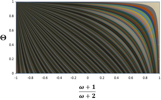
Figure 1: Contour plot of $\gamma_{\text{exact}}$ in terms of $\varTheta$ and $\frac{\omega+1}{\omega+2}$, for the physical range of $\varTheta\in[0,1]$ and $\omega\in(-3/2,+\infty)$. The latter is translated to $\frac{\omega+1}{\omega+2}\in(-1,1)$. Contours are equally spaced in 0.005 increments. Note that for a given contour, the corresponding value of $\gamma_{\,\text{exact}}$ equals to that on the abscissa axis where the contour intersects it. A value of $\gamma_{\,\text{exact}}$ approximately 1 can infer that $\frac{\omega+1}{\omega+2}\approx 1$ (i.e., $\omega\gg 1$) or $\varTheta\approx 1$ (i.e., ultra-relativistic matter).

The previous conclusions were implicit in Ref. [26], in which the general multi-tensor-scalar case was considered. Nevertheless, we have provided here, for the first time, an explicit and ready-for-use compact formula (21) for the $\gamma$ parameter in the BD case. Such an explicit expression immediately elucidates how a given stellar interior model directly impacts the orbital dynamics of bodies orbiting at intermediate distances. Besides, the (16)–(18) integrals also fully determine the parameters of the Brans Class I solution (9), which then also allow to determine orbital dynamics in the strong field region of the star.

Rewriting (21) as $1-\gamma_{\,\text{exact}}=\frac{1-\Theta}{\omega+2+\left(\omega+1\right)\Theta}$ shows that, as illustrated in Figure 1, having $\gamma_{\,\text{exact}}$ close to $1$ (GR mimicking) requires either large $\omega$ (BD itself close to GR) or $\Theta$ close to $1$ (ultra-relativistic matter). On the other hand, (21) also yields

$$\gamma_{\,\text{exact}}-\frac{\omega+1}{\omega+2} =\frac{\left(2\omega+3\right)\Theta}{\left(\omega+2\right)\left[\omega+2+\left(\omega+1\right)\Theta\right]}$$ (22)

$$=\left\{\begin{array}[]{l}\frac{2\omega+3}{\left(\omega+2\right)^{2}}\Theta+O\left(\Theta^{2}\right)<\frac{2\Theta}{\omega}+O\left(\Theta^{2}\right)\\ \frac{2}{\omega\left(1+\Theta\right)}\Theta+O\left(\frac{1}{\omega^{2}}\right)<\frac{2\Theta}{\omega}+O\left(\frac{1}{\omega^{2}}\right)\end{array}\right.$$ (25)

(the upper bound by $2\Theta/\omega$ being satisfied for positive $\omega$). At first glance, since $\Theta$ is strongly expected to be much smaller than 1 for the Sun, there is no significant impact to expect in Solar System dynamics, since $\omega\gg 1$ seems unavoidable. Indeed, if $\omega$ were not much larger than 1, or were of order of unity, a small $\left(1-\Theta\right)$, i.e. $\varTheta\approx 1$, would be required since $\left(1-\gamma\right)$ is experimentally known to be small.

As a final remark, let us stress that the calculation presented here reveals an important consequence. It shows that, even in the spherical case, motions around a compact star do not only carry information on the gravity theory, but that this information is mixed with features of the star’s structure beyond its only mass. The point has some acquaintance with the loss of the Birkhoff theorem in BD. Indeed, this loss means that the pulsations (or the collapse) of a non static spherical star affect orbital motions around it, which therefore are no longer just determined by the star’s mass (for a given $\omega$ parameter, i.e. BD theory). The notable point here is that, also in the static case, the sole mass knowledge does not permit to know what PN orbital motions around the star are. Knowing more is needed.

References

- [1] C. M. Will, The confrontation between general relativity and experiments. Living Rev. Relativ. 17, https://doi.org/10.12942/lrr-2014-4, 4 (2014).
- [2] C. M. Will, Theory and Experiment in Gravitational Physics (Cambridge University Press, 2018).
- [3] R. A. Hulse and J. H. Taylor, Astrophys. J. Lett. 195, L51 (1975).
- [4] N. Ashby, Relativity in the Global Positioning System. Living Rev. Relativ. 6, https://doi.org/10.12942/lrr-2003-1 (2003).
- [5] O. Bertolami and J. Páramos, IJMPD 20, 1617 (2011).
- [6] A. M. Ghez, B. L. Klein, M. Morris, and E. E. Becklin, ApJ 509, 678 (1998).
- [7] A. G. Riess et al, Astron. J. 116, 1009 (1998).
- [8] S. Perlmutter et al, Astrophys. J. 517, 565 (1999).
- [9] R. Genzel et al., Nature 425, 934 (2003).
- [10] K. Akiyama et al., ApJL, 875, L1 to L6 (2019).
- [11] K. Akiyama et al., ApJL, 910, L12 and L13 (2021).
- [12] K. Akiyama et al., ApJL, 930, L12 to L21 (2022).
- [13] A.C. Fabian and A.N. Lasenby, arXiv:1911.04305 (2019).
- [14] B. P. Abbott et al., Phys. Rev. Lett. 116, 061102 (2016).
- [15] C. Brans and R. H. Dicke, Phys. Rev. 124, 925 (1961).
- [16] R. H. Dicke, Phys. Rev. 125, 2163 (1962).
- [17] C. H. Brans, Phys. Rev. 125, 2194 (1962).
- [18] P. G. Bergmann, Int. J. Theor. Phys. 1, 25 (1968).
- [19] K. J. Nordtvedt, Astrophys. J. 116, 1059 (1970).
- [20] R. V. Wagoner, Phys. Rev. D 1 3029 (1970).
- [21] Y. Fujii and K. Maeda, The scalar-tensor theory of gravitation (Cambridge University Press, 2003).
- [22] V. Faraoni, Cosmology in scalar-tensor gravity (Kluwer Academic Publishers, 2004).
- [23] S. Capozziello and V. Faraoni, Beyond Einstein’s gravity, Fundamental Theories of Physics, volume 170, Springer (2011).
- [24] T. Damour and K. Nordtvedt, Phys. Rev. Lett. 70, 2217 (1993).
- [25] T. Damour and K. Nordtvedt, Phys. Rev. D 48, 3436 (1993).
- [26] T. Damour and G. Esposito-Farese, Class. Quant. Grav. 9, 2093 (1992).