Fair Concurrent Training of Multiple Models in Federated Learning

Abstract

Federated learning (FL) enables collaborative learning across multiple clients. In most FL work, all clients train a single learning task. However, the recent proliferation of FL applications may increasingly require multiple FL tasks to be trained simultaneously, sharing clients’ computing and communication resources, which we call Multiple-Model Federated Learning (MMFL). Current MMFL algorithms use naïve average-based client-task allocation schemes that can lead to unfair performance when FL tasks have heterogeneous difficulty levels, e.g., tasks with larger models may need more rounds and data to train. Just as naïvely allocating resources to generic computing jobs with heterogeneous resource needs can lead to unfair outcomes, naïve allocation of clients to FL tasks can lead to unfairness, with some tasks having excessively long training times, or lower converged accuracies. Furthermore, in the FL setting, since clients are typically not paid for their training effort, we face a further challenge that some clients may not even be willing to train some tasks, e.g., due to high computational costs, which may exacerbate unfairness in training outcomes across tasks. We address both challenges by firstly designing FedFairMMFL, a difficulty-aware algorithm that dynamically allocates clients to tasks in each training round. We provide guarantees on fairness and FedFairMMFL’s convergence rate. We then propose a novel auction design that incentivizes clients to train multiple tasks, so as to fairly distribute clients’ training efforts across the tasks. We show how our fairness-based learning and incentive mechanisms impact training convergence and finally evaluate our algorithm with multiple sets of learning tasks on real world datasets.

I Introduction

Federated learning (FL) enables multiple devices or users (called clients) to collectively train a machine learning model  [1, 2, 3, 4], with data staying at the user side. Several recent works have demonstrated FL’s potential in many applications, such as smart homes [2, 3], analyzing healthcare data [5], and next word prediction [6]. Despite the large and growing set of FL applications, however, the vast majority of FL research assumes that each client only trains one learning task during FL. In practice, clients may concurrently train multiple tasks, e.g., if smartphones contribute to training both next-word prediction and advertisement recommendation models, or if hospitals contribute to training separate prediction models for heart disease and breast cancer. Clients could also train multiple versions of a model, in order to select the best-performing one for deployment, e.g., training many different neural network architectures on the same data. We call this setting in which FL clients simultaneously train multiple tasks, Multiple-Model Federated Learning (MMFL) [7, 8, 9, 10, 11]. Training multiple tasks in one FL setting amortizes the real-world costs of recruiting clients and coordinating the training time across clients, improving resource efficiency.

Since FL clients, especially mobile or Internet of Things devices, may be resource-constrained [1], they may not be able to train every FL task at the same time. Thus, we must allocate clients to the different tasks in each training round. Prior work on MMFL has shown that with careful selection of clients for each task in each training round, concurrent training yields comparable accuracy to training tasks separately [7]. These works, however, seek to optimize the average task accuracy or training time, and often assume that training tasks have similar difficulties, e.g., training multiple copies of the same model [8, 7]. In practice, however, FL tasks may be requested by different entities and users, and it is important to ensure comparable convergence time and converged accuracies across tasks of varied difficulty levels. Hospitals, for example, may wish to concurrently train prediction models for different diseases, without favoring one disease’s model over another. Likewise, in applications like autonomous driving, improving the worst-performing FL task helps to improve the overall quality of experience for users. Indeed, even if the multiple tasks are different models trained by the same FL operator, the operator will not know which model performs best until the training of all models is complete: we therefore would want to dynamically allocate clients to tasks so as to optimize the performance of the worst-performing task, which is accomplished by optimizing for fairness. To the best of our knowledge, we are the first to extend the MMFL setting to consider fair training of concurrent FL models.

I-A Research Challenges in Fair MMFL

In considering fairness across multiple different models, we seek to ensure that each model achieves comparable training performance, in terms of their converged accuracies, or the time taken to reach threshold accuracy levels. The first challenge to doing so is that the multiple models can have varying difficulties and thus require different amounts of data and computing resources to achieve the same accuracy. Existing MMFL training algorithms, e.g., the round-robin algorithm proposed in [7], allocate clients to tasks uniformly, or assume that tasks have similar or the same difficulty, e.g., training multiple copies of the same model [8]. However, while such strategies arguably achieve fairness, or at least equality, in resource (i.e., client) allocation to different models, they may lead to “unfair” outcomes. For example, smart home devices may train simple temperature prediction models that take low-dimensional timeseries as input data, as well as complex person identification ones that use high-dimensional image input data [3]. Allocating equal resources to each model may then yield poor performance for the more difficult ones.

Much work in computer systems and networks has focused on fairness in allocating resources to different computing jobs or network flows, given their heterogeneous resource requirements [12, 13, 14]. Simply applying these allocation algorithms to MMFL, however, is difficult: here, each “resource” is a client, and the performance improvement realized by allocating this client to a given model’s training task is unknown in advance and will change over time. This is because it depends on the current model state and the data distribution across clients, both of which are highly stochastic. We must therefore handle significant uncertainty and dynamics in how much each client contributes to each task’s training performance.

Finally, purely viewing MMFL fairness as a matter of assigning clients to tasks ignores the fact that clients may not be equally willing to contribute resources to each model. For example, smartphone users may benefit from better next-word prediction models if they text frequently, but may derive limited benefit from a better ad recommendation model. Users may refuse to compute updates if they judge that associated computing costs outweigh personal benefits. If multiple users prefer one model over another, then the disfavored model will overfit to users willing to train it, again leading to an unfair outcome. In an extreme case, no users may be assigned to train this task at all. Prior work[15] has proposed mechanisms to incentivize clients to help train multiple non-simultaneously trained FL models, but the focus was on optimizing the task take-up rate, instead of ensuring that clients are fairly distributed across models.

I-B Our Contributions

Our goal is to design methods to ensure fair concurrent training of MMFL, addressing the challenges above. To do so, we utilize the popular metric of $\alpha$-fairness, commonly used for fair resource allocation in networking [16] and previously proposed to measure fairness across clients in training a single FL model [17]. We use $\alpha$-fairness and Max-Min fairness (a special case of $\alpha$-fairness when $\alpha\rightarrow\infty$ [16]) to design novel algorithms that both incentivize clients to contribute to FL tasks and adaptively allocate these incentivized clients to multiple tasks during training. Intuitively, these algorithms ensure that client effort is spread across the MMFL tasks in accordance with their difficulty, helping to achieve fairness with respect to task performances. After discussing related works in Section II, we make the following contributions:

• We first suppose that all clients are willing to train all models, and propose FedFairMMFL, an algorithm to fairly allocate clients to tasks (i.e., models) in Section III. Our algorithm dynamically allocates clients to tasks according to the current performance levels of all tasks. We design FedFairMMFL to approximately optimize the $\alpha$-fairness of all tasks’ training accuracies.

• From the perspective of a single model, our client-task allocation algorithm in MMFL can be viewed as a form of client selection. We therefore adapt and refine convergence guarantees from analyses of client selection in FL to analyze the convergence of MMFL tasks under FedFairMMFL in Section IV, showing that FedFairMMFL preferentially accelerates convergence of more difficult tasks (Theorem 4 and Corollary 5) and allows each model’s training to converge (Corollary 6).

• We next suppose that clients may have unequal interest in training different tasks and may need to be incentivized. We discuss Budget-Fairness and Max-min Fairness, and we propose a max-min fair auction mechanism to ensure that a fair number of clients are incentivized across tasks. We show that it incentivizes truthful client bids with high probability (Theorem 8 and Corollary 9). We also show that it leads to more fair outcomes: it allocates more clients to each model, compared to other auction mechanisms that either ignore fairness or allocate the same budget to each task (Corollary 10). Following which, we provide a convergence bound showing how our proposed incentive mechanisms coupled with FedFairMMFL impact the convergence rate (Theorem 11).

• We finally validate our client incentivization and allocation algorithms on multiple FL datasets. Our results show that our algorithm achieves a higher minimum accuracy across tasks than random allocation and round robin baselines, and a lower variance across task accuracy levels, while maintaining the average task accuracy. Our max-min client incentivization further improves the minimum accuracy in the budget-constrained regime.

We discuss future directions and conclude in Section VII.

II Related Work

We distinguish our MMFL setting from that of multi-task learning (MTL), in which multiple training tasks have the same or a similar structure [18], e.g., a similar underlying lower rank structure. Unlike clustered FL [19, 20], our work is different from combining MTL with FL, instead we consider multiple distinct learning tasks. Our analysis of MMFL performance is closer to prior convergence analysis of client selection in FL [21, 22, 23]. We adapt prior work on FL convergence to reveal the relationships between model convergence and our definition of fairness across tasks.

Past work on multi-model federated learning also aims to optimize the allocation of clients to model training tasks. To the best of our knowledge, we are the first to explicitly consider fairness across the different tasks. Some algorithms focus on models with similar difficulties, for which fairness is easier to ensure [7], while other works propose reinforcement learning [24], heuristic [9], or asynchronous client selection algorithms [10] to optimize average model performance. Other work optimizes the training hyperparameters [25] and allocation of communication channels to tasks [21].

Fair allocation of multiple resources has been considered extensively in computer systems and networks  [26, 12, 13]. In crowdsourcing frameworks, the fair matching of clients to tasks has been studied in energy sensing [27], delivery [28], and social networks [29]. However, unlike MMFL tasks, individual crowdsourcing tasks generally do not need multiple clients. Fair resource allocation across tasks in FL differs from all the above applications as the amount of performance improvement realized by allocating one (or more) clients to a given model’s training task is unknown and stochastic, dependent on the model state and clients’ data distributions. In FL, fairness has generally been considered from the client perspective, e.g., accuracies or contribution when training a single model [17, 30], and not across distinct training tasks.

Many incentive mechanisms have been proposed for FL and other crowdsourcing systems [31, 32, 33, 34, 35], including auctions for clients to participate in many FL tasks [15]. To the best of our knowledge, this is the first time client incentives have aimed to ensure fair training of multiple tasks in MMFL.

III Fair Client Task Allocation for Multiple-Model FL

We aim to train multiple models (i.e., tasks) concurrently, such that there is fair fair training performance across models, e.g., in terms of the time taken, or converged accuracies. Models may be trained on distinct or the same datasets. This performance is a function of which clients train which model at which training round. In this section, we assume clients always train any given model upon request and propose a client-model (i.e., client-task) allocation scheme that enables fair training of the multiple tasks. In Sec. V, we introduce auction mechanisms, which incentivize clients to commit to tasks at a fair rate across tasks, before training begins (Fig. 1).

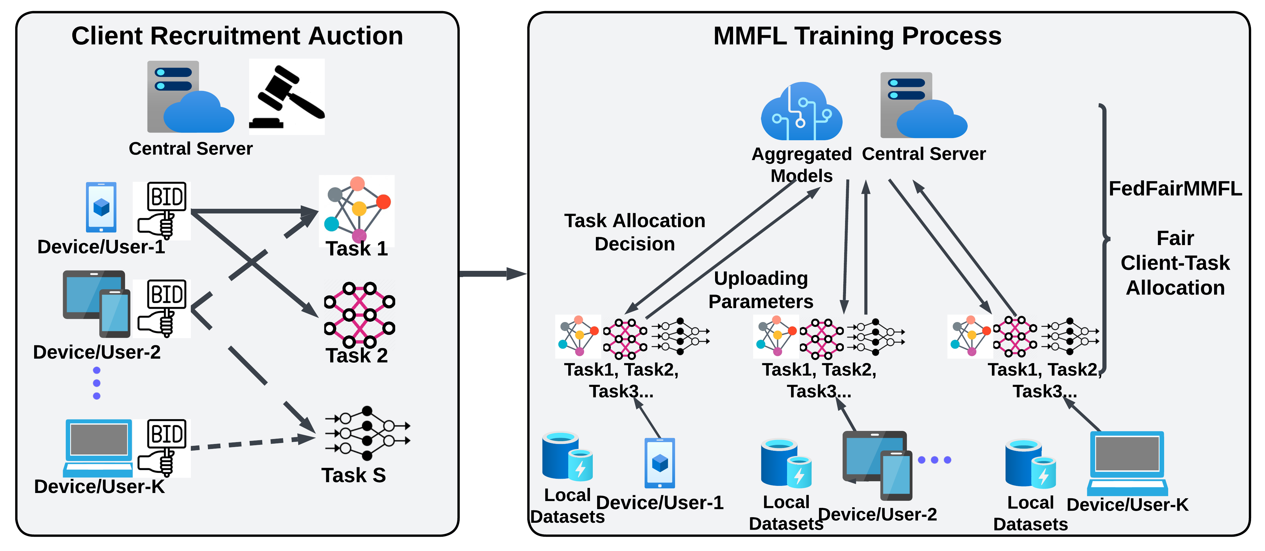
Figure 1: Fair Multiple Model Federated Learning to ensure that each model achieves comparable training performance: The pipeline’s first part involves incentive-aware client recruitment auctions to ensure a fair take-up rate over tasks. This is followed by a difficulty-aware client-task allocation scheme that allocates tasks to clients based on the current loss levels of all tasks.

MMFL framework: Consider $K$ clients collaboratively training $S$ distinct machine learning tasks in MMFL (Fig. 1). If $S=1$, our setting reduces to traditional FL. Each client is equipped with local data for training each task. All clients can communicate with a central server that maintains a global model $\textbf{w}_{s}$ for each task $s\in\mathbb{S}$. Let each client $k$’s local loss over its local dataset $\mathcal{D}_{k,s}$ for task $s$ be $F_{k,s}(\textbf{w}_{s})=\sum_{d\in\mathcal{D}_{k,s}}\ell\left(d,\textbf{w}_{s}\right)/\left|\mathcal{D}_{k,s}\right|$, where $\ell$ is a loss function that measures the accuracy of the model $\textbf{w}_{s}$ on data point $d$. We then define the global loss for task $s$ as a weighted sum over the local losses: $f_{s}(\textbf{w}_{s})=\sum_{k=1}^{K}p_{k,s}F_{k,s}(\textbf{w}_{s})$, where $p_{k,s}=\frac{\left|\mathcal{D}_{k,s}\right|}{\sum_{k}\left|\mathcal{D}_{k,s}\right|}$ is the fraction of training data for task $s$ that resides at client $k$. Similar to traditional FL, in MMFL, the usual aim is to minimize the sum of losses [10]:

$$\min_{\textbf{w}_{1},\textbf{w}_{2},...,\textbf{w}_{S}}\sum_{s=1}^{S}f_{s}(\textbf{w}_{s}),$$ (1)

Fairness over tasks: We introduce fairness into this objective by utilizing the celebrated $\alpha$-fair utility function often employed to ensure fair network resource allocation [16, 13]. Viewing the loss of each model as an inverse “utility,” we then define our $\alpha$-fair MMFL objective as

$$\min_{\textbf{w}_{1},\textbf{w}_{2},...\textbf{w}_{S}}g^{\alpha}\left(\textbf{w}_{1},\textbf{w}_{2},...\textbf{w}_{S}\right)\equiv\sum_{t=1}^{S}f_{s}^{\alpha}(\textbf{w}_{t}),$$ (2)

where $f_{s}^{\alpha}$ is task $s$’s $\alpha$-fair global loss function. This objective function helps to improve the uniformity of the converged losses, as we will analytically show in Section IV. Here the parameter $\alpha\in[1,\infty)$ controls the emphasis on fairness; for $\alpha=1$, the objective is to minimize the average global loss across tasks. As $\alpha$ grows, we put more emphasis on fairness, because analytically, a higher $\alpha$ will give higher priority to the terms in the objective with larger $f_{s}$, during minimization.

To solve (2) within the FL framework, we will use gradient descent to design a training algorithm given the gradient

$$\nabla_{\textbf{w}_{s}}g=\alpha f_{s}^{\alpha-1}(\textbf{w}_{s})\sum_{k}p_{k}\nabla F_{k,s}(\textbf{w}_{s}).$$ (3)

FedFairMMFL training (Algorithm 1): Our MMFL training begins with the initialization of the global model weights $\textbf{w}_{s}$ for all tasks, along with an initial random client-task allocation (line 1). The algorithm then enters a loop over global rounds (lines 2-15). During each global round $t$, $m=C\times|\mathcal{C}|$ clients are active (line 3). Here $C$ is the rate at which clients are active. For all active clients, task allocation happens. We let $Sel_{s}(t)$ denote the set of clients allocated to task $s$ in round $t$, dropping the subscript $s$ if it is clear from context. Following prior work on MMFL [7, 8, 24], we allocate each client to at most one task during each training round, i.e., the $Sel_{s}(t)$ are disjoint across tasks $s$. For example, mobile clients or other resource constrained devices may be performing other background tasks, e.g., running multiple applications, and thus may not have the computing power or battery to complete training rounds of multiple tasks.

Intuitively, uniform client-task allocation methods, like random or round robin allocation [8], will train simpler tasks faster, since they allocate an equal number of clients to each task, in expectation. We would instead like to ensure tasks are trained at more similar rates (i.e., achieve more fair performance) with a difficulty-aware client-task allocation algorithm, in which more users are allocated to tasks that currently have a higher loss compared to other tasks. We can do so by inspecting the gradient of our MMFL objective in (3). Since resource-constrained clients can only compute gradients for one task per training round, we cannot exactly compute these gradients. Instead, we will assign each client to contribute to the gradient $\nabla F_{k,s}(\textbf{w}_{s})$ for each task $s$ at a probability in proportion to its weight for that task, i.e., proportional to $\alpha f_{s}(\textbf{w}_{s})^{\alpha-1}p_{k}$. We therefore allocate a task to each client according to the probability vector (lines 4-5):

$$\textbf{p}=\left[\frac{f^{\alpha-1}_{1}}{\sum_{s\in\mathbb{S}}f^{\alpha-1}_{s}},\frac{f^{\alpha-1}_{2}}{\sum_{s\in\mathbb{S}}f^{\alpha-1}_{s}},...,\frac{f^{\alpha-1}_{S}}{\sum_{s\in\mathbb{S}}f^{\alpha-1}_{s}}\right],$$ (4)

This allocation fulfills our intuition: tasks currently with higher losses $f_{s}$ have a higher probability of being allocated clients. For example, when $\alpha\rightarrow\infty$, all clients will be allocated to the worst performing task, and when $\alpha=1$, allocation will be uniform. In Section IV, we formalize this intuition by deriving a convergence bound for each task using FedFairMMFL. This selection scheme is unbiased across clients: each client is equally likely to train a given task.

Given the clients allocated to each task $s$ at time $t$, $Sel_{s}(t)$, the server then sends the latest global model weights $\textbf{w}_{s}(t)$ to task $s$’s allocated clients (lines 7-8). Each client then trains its task on its corresponding local dataset by running $\tau$ SGD steps on the local loss $F_{k,s}$ of its assigned task $s$, as in traditional FL [1] (line 9). Let $\textbf{w}_{k,s}(t)$ denote the updated local model for active client $k$ on its allocated task $s$. Each active client then uploads $\textbf{w}_{k,s}(t)$ to the server (line 9), which aggregates the model parameters to synchronize the global model. This aggregation uses weights $p_{k,Sel}=p_{k}/\sum_{k\in Sel}p_{k^{\prime}}$ for each client $k$ (line 12), where $Sel$ is the set of clients training task $s$ in this training round. The server then obtains the global loss for each task $f_{s}$, to guide allocation in the next training round (line 13). The next training round then begins.

Algorithm 1 FedFairMMFL: Fair Training of Multiple Models in Federated Learning

1:Initialization: The global model weights $\textbf{w}_{s}$, for all tasks, initial random client-task allocation.

2:for $Globalepoch=1,2,\ldots$ do

3:    $m=C\times|\mathcal{C}|$ clients are active.

4:    Server determines task allocation for active clients,

5:    based on $\mathbf{p}=\left[{f^{\alpha-1}_{1}}/{\sum_{s\in\mathbb{S}}f^{\alpha-1}_{s}},...\right]$ (Eq. 4).

6:    for all active clients $k$ do

7:         Server sends latest global model weights of task $s$,

8:         $\textbf{w}_{s}$ to clients allocated.

9:         Client performs local SGD (stochastic gradient descent) $\tau$ times for allocated task, optimizing $\textbf{w}_{k,s}$, and uploads $\textbf{w}_{k,s}$ to the server.

10:    end for

11:    for all tasks $s\in\mathbb{S}$ do

12:         Server aggregates $\textbf{w}_{s}\leftarrow\textbf{w}_{s}-\eta_{t}\sum_{k}p_{k,Sel}\nabla F_{k}(\textbf{w}_{s})$.

13:         Obtain global accuracy $f_{s}$ for task $s$.

14:    end for

15:end for

IV Fairness and Convergence Guarantees

We now analyze FedFairMMFL’s performance. The full versions of all our proofs are in our Technical Report [36].

IV-A Fairness Guarantees

We first analyze the optimal solution to our fairness objective (2) to show that it reduces the variation in training accuracy, which intuitively improves fairness across tasks. Firstly, we denote $\textbf{w}^{*}_{s,\alpha}=G^{\alpha}=\min_{\textbf{w}_{s}}g^{\alpha}(\{\textbf{w}_{s}\})$, where

$$G^{\alpha}=\min_{\mathbf{\textbf{w}_{s}}}\bigg{\{}\bigg{(}\frac{1}{S}\sum^{S}_{s=1}f^{\alpha}_{s}(\textbf{w}_{s})\bigg{)},\text{s.t.}\sum_{s}a_{k,s}=1\ \forall k\ \forall t\bigg{\}},$$ (5)

where $a_{k,s}$ indicates that user $k$ trains task $s$ during epoch $t$ and $\sum_{s}a_{k,s}=1\ \forall k\ \forall t$ expresses the constraint that each client trains 1 task each epoch, and $\textbf{w}^{*}_{s,\alpha}$ is the global optimal solution when parameter $\alpha$ is used. In other words, $G^{\alpha}$ represents the optimal value of our MMFL objective (2).

To motivate the choice of $\alpha$, we show that for $\alpha=1,2$, a higher $\alpha$ puts more emphasis on fairness: we relate this $\alpha$-fairness metric to the well-known variance and cosine similarity metrics for similarity across task accuracies.

Lemma 1 (Fairness and Variance).

$\alpha=2$ yields a smaller variance in the task accuracies than $\alpha=1$:

$$\textbf{Var}(f_{1}(\textbf{w}_{1,2}^{*}),...,f_{n}(\textbf{w}_{n,2}^{*}))\leq\textbf{Var}(f_{1}(\textbf{w}_{1,1}^{*}),...,f_{n}(\textbf{w}_{n,1}^{*})).$$

Proof Sketch: We followed the outline of the proof if [17]. As we are interested in task fairness, unlike [17], we replace client loss functions with the global task loss functions $f_{s}(\textbf{w}_{s,\alpha})$ in our derivations. We next combine the definitions of the variance and $\textbf{w}_{s,\alpha}^{*}$ in Eq. (5) to obtain our result. ∎

Next, we use the definition of cosine similarity to show that $\alpha=2$ results in a fairer solution than $\alpha=1$ (non-fairness).

Lemma 2 (Fairness and Cosine Similarity).

$\alpha=2$ results in a higher cosine similarity across tasks than $\alpha=1$, i.e.

$$\frac{\frac{1}{S}\sum_{s=1}^{S}f_{s}(\textbf{w}_{s,2}^{*})}{\sqrt{\frac{1}{S}\sum_{s=1}^{S}f_{s}^{2}(\textbf{w}_{s,2}^{*})}}\geq\frac{\frac{1}{S}\sum_{s=1}^{S}f_{s}(\textbf{w}_{s,1}^{*})}{\sqrt{\frac{1}{S}\sum_{s=1}^{S}f_{s}^{2}(\textbf{w}_{s,1}^{*})}}.$$ (6)

Proof Sketch: We followed the outline of [17]. Unlike [17], we are concerned with fairness across tasks, hence we replace user loss functions with the global task loss functions in our derivations. We further use the definition of cosine similarity, and the definition of $\textbf{w}_{s,\alpha}^{*}$ and $G^{\alpha}(\textbf{w}_{s})$ to obtain our result.∎

IV-B Convergence Guarantees

Here, we analyze the convergence of training tasks under our client-task allocation algorithm, showing that it preferentially accelerates training of tasks with higher losses and that each task will converge. We prove convergence by taking the perspective of a single task in MMFL, without loss of generality.

We first characterize $B_{Sel}^{s}$, the probability that a specific set of clients $Sel$ is allocated (i.e., selected) for a specific task $s$ by our algorithm FedFairMMFL.

$$B_{Sel}^{s}(\alpha)=\textstyle\left(\frac{f_{s}^{\alpha}(t)}{\sum_{s^{\prime}\in S}f_{s^{\prime}}^{\alpha}(t)}\right)^{|Sel|}\left(1-\frac{f_{s}^{\alpha}(t)}{\sum_{s^{\prime}\in S}f_{s^{\prime}}^{\alpha}(t)}\right)^{K-|Sel|}$$ (7)

$B_{Sel}^{s}(\alpha)$ depends on the losses of all tasks $s\in S$, and our $\alpha$-fair parameter $\alpha$. Next we introduce $\Gamma_{s}$, the gap between the loss evaluated at the global optimum $\mathbf{w}_{s}^{*}$, and the loss evaluated at client $k$’s optimal $\mathbf{w}^{*}_{k,s}$, for task $s$: $\Gamma_{s}=\sum_{k=1}^{K}p_{k}(F_{k,s}(\mathbf{w^{*}}_{s})-F_{k,s}(\mathbf{w}^{*}_{k,s}))=f_{s}^{*}-\sum_{k=1}^{K}p_{k}F_{k,s}^{*}.$ We further characterise the selection skew $\rho^{\alpha}(B^{s}_{Sel},\mathbf{w}^{\prime})$. The selection skew is a ratio of the expected ‘local-global objective gap’ of the selected clients under FedFairMMFL over the ‘local-global objective gap’ of all $K$ clients, where $\textbf{w}^{\prime}$ is the point at which $F_{k,s}$ and $f_{s}$ are evaluated. This skew depends on the expectation of client allocation combinations, and hence on $B_{Sel}^{s}$ and the $\alpha$-fair parameter $\alpha$:

$$\rho^{\alpha}(B^{s}_{Sel},\mathbf{w}^{\prime})$$

$$=\frac{\sum_{Sel\in\mathbb{S}}{\color[rgb]{0,0,0}B_{Sel}^{s}(\alpha)}\sum_{k\in Sel}{\color[rgb]{0,0,0}\frac{p_{k}}{\sum_{k^{\prime}\in Sel}p_{k’}}}(F_{k,s}(\textbf{w}_{s}^{{}^{\prime}})-F_{k,s}^{*})}{f_{s}(\mathbf{w}^{\prime})-\sum_{k=1}^{K}p_{k}F_{k,s}^{*}}$$

We use $\overline{\rho}^{\alpha}$ and $\underline{\rho}^{\alpha}$ respectively to denote upper and lower bounds on the selection skew throuhgout the training. Recall that $\tau$ denotes the number of SGD epochs in local training. We then introduce the following assumptions used in our convergence analysis, which are standard in the FL literature [22].

Assumption 1: $F_{1,s},..,F_{k,s}$ are L-smooth, i.e. $F_{k,s}(\mathbf{v})\leq F_{k,s}(\mathbf{w})+(\mathbf{v}-\mathbf{w})^{T}\nabla F_{k,s}(\mathbf{w})+\frac{L}{2}\|\mathbf{v}-\mathbf{w}\|^{2},\ \forall\mathbf{v}$ and $\mathbf{w}$.

Assumption 2: $F_{1,s},..F_{k,s}$ are $\mu$-strongly convex, i.e. $F_{k,s}(\mathbf{v})\geq F_{k,s}(\mathbf{w})+(\mathbf{v}-\mathbf{w})^{T}\nabla F_{k,s}(\mathbf{w})+\frac{\mu}{2}\|\mathbf{v}-\mathbf{w}\|^{2}$, for all $\mathbf{v}$ and $\mathbf{w}$. Note that $\mu\leq L$ in from Assumption 1.

Assumption 3: For all clients $k$, for the minibatch $\xi_{k,s}$ uniformly sampled at random, the stochastic gradient is unbiased: $\mathbb{E}[g_{k,s}(\mathbf{w}_{k,s},\xi_{k,s})]=\nabla F_{k,s}(\textbf{w}_{k,s})$, and its variance is bounded: $\mathbb{E}\|g_{k,s}(\mathbf{w}_{k,s},\xi_{k,s})]-\nabla F_{k,s}(\textbf{w}_{k,s})\|^{2}\leq\sigma^{2}$.

Assumption 4: Bounded stochastic gradient. For all clients $k$, the expected square norm of the stochastic gradient is bounded $\mathbb{E}\|g_{k,s}(\textbf{w}_{k,s},\xi_{k,s})\|^{2}\leq G^{2}$.

Lemma 3 (Local and Global Model Discrepancy).

The expected average discrepancy between the global model for task $s$, $\overline{\textbf{w}}^{(t)}_{s}$ and client $k$’s model for $s$, $\textbf{w}_{k,s}^{(t)}$, under selection $k\in Sel(t)$, can be bounded as

$$\mathbb{E}[\sum_{k\in Sel(t)}\frac{p_{k}}{\sum_{k^{\prime}\in Sel(t)}p_{k^{\prime}}}\|\overline{\textbf{w}}^{(t)}_{s}-\textbf{w}_{k,s}^{(t)}\|^{2}]$$ (8)

$$\leq 16\eta_{t}^{2}\tau^{2}G^{2}\sum_{Sel(t)\in\mathbb{S}(t)}B_{Sel(t)}^{s}(\alpha)P^{k,2}_{Sel(t)}$$ (9)

where $P^{k,2}_{Sel(t)}=\sum_{\begin{subarray}{c}k\neq k^{\prime},\\ k,k^{\prime}\in Sel(t)\end{subarray}}p_{k}\frac{p_{k^{\prime}}}{(\sum_{k^{{}^{\prime\prime}}\in Sel(t)}p_{k^{\prime\prime}})^{2}}$.

In the next theorem, without loss of generality we show the convergence rate of a task in the MMFL setting under FedFairMMFL, and show its dependence on the relative loss levels of all tasks. When the prevailing loss level of task $s$ is higher, its convergence will be sped up under our algorithm.

Theorem 4 (Model Parameter Convergence).

Suppose we use learning rate $\eta_{t}$ at each round $t$. Under Assumptions 1-4, the progress of task $s$’s global parameters at round $t+1$, $\overline{\textbf{w}}_{s}^{(t+1)}$, towards the optimal parameters $\textbf{w}^{*}$: $\mathbb{E}\left[\|\overline{\textbf{w}}^{(t+1)}_{s}-\textbf{w}_{s}^{*}\|^{2}\right]$ is upper-bounded by

$$\left[1-\eta_{t}\mu(1+\frac{3\overline{\rho}^{\alpha}}{8})\right]\mathbb{E}[\|\overline{\textbf{w}}^{(t)}-\textbf{w}^{*}_{s}\|^{2}]+2\eta_{t}\Gamma_{s}(\tilde{\rho}^{\alpha}-\overline{\rho}^{\alpha})$$

$$+\eta_{t}^{2}\sigma^{2}\sum_{Sel(t)\in\mathbb{S}(t)}\sum_{k\in Sel(t)}B_{Sel(t)}^{s}(\alpha)\left(\frac{p_{k}}{\sum_{k^{\prime}\in Sel(t)}p_{k’}}\right)^{2}$$

$$+\eta_{t}^{2}\left(32\tau^{2}G^{2}+6\overline{\rho}^{\alpha}L\Gamma_{s}\right).$$ (10)

Proof Sketch: We adapted the outline of [22]’s proof to incorporate our distinct client selection scheme, which unlike [22]’s proof requires explicitly quantifying the impact of $Sel(t)$ and $B^{s}_{Sel}$ (Eq. 7) through various bounds on the loss function gradients. In the rest of our proof, we add and subtract multiple expressions involving the gradients, bound the various terms, and incorporate Lemma 3’s result. ∎

In tracking the impact of our client-task allocation on the convergence in Theorem 4’s proof, we also reveal how the convergence bound in (4) depends on our client-task allocation algorithm, in particular the parameter $\alpha$ and the current task losses. This result not only helps us to prove the convergence of our FedFairMMFL training algorithm, but also provides additional justification for our client-task allocation strategy: Mathematically, tasks that are further from the optimum (i.e., with a larger $\mathbb{E}[\|\overline{\textbf{w}}^{(t)}-\textbf{w}^{*}_{s}\|^{2}$) should be allocated clients to reduce the right-hand side of (4) to equalize the progress across all tasks, which agrees with our algorithm. In Corollary 5, we show that under certain conditions on $p_{k}$, as $\alpha$ increases, the term with $B^{s}_{Sel}(\alpha)$ decreases, hence controlling the task’s progress towards its optimum.

Corollary 5 (Fairness and Convergence).

Suppose that all of the $p_{k}=\frac{1}{K}$ and consider task $s$ that has the highest loss $f_{s}\left(\textbf{w}_{s}(t+1)\right)$. Then as $\alpha$ increases, the term $\eta_{t}^{2}\sigma^{2}\sum_{Sel\in\mathbb{S}(t)}\sum_{k\in Sel}B_{Sel}^{s}(\alpha)\left(\frac{p_{k}}{\sum_{k^{\prime}\in S(t)}p_{k’}}\right)^{2}$ in the right-hand side of (4) decreases.

Proof.

Let $\overline{f}_{s}(\alpha)=\frac{f_{s}\left(\textbf{w}_{s}(t+1)\right)^{\alpha}}{\sum_{s^{\prime}}f_{s^{\prime}}\left(\textbf{w}_{s}(t+1)\right)^{\alpha}}$. When $p_{k}=\frac{1}{K}$, we can rewrite $\sum_{Sel\in\mathbb{S}(t)}\sum_{k\in Sel}B_{Sel}^{s}(\alpha)\left(\frac{p_{k}}{\sum_{k^{\prime}\in S(t)}p_{k’}}\right)^{2}$ as $\sum_{j=1}^{K}\frac{1}{j}\left(\overline{f}_{s}(\alpha)\right)^{j}\left(1-\overline{f}_{s}(\alpha)\right)^{K-j}{K\choose j}$.
Since $\sum_{j=1}^{K}\left(\overline{f}_{s}(\alpha)\right)^{j}\left(1-\overline{f}_{s}(\alpha)\right)^{K-j}{K\choose j}=1$, we can view this as a weighted average of $1,\frac{1}{2},\ldots,\frac{1}{K}$. It then suffices to show that, as $\alpha$ increases, we place more weight on smaller terms. Note that $\frac{d}{d\alpha}\left(\left(\overline{f}_{s}(\alpha)\right)^{j}\left(1-\overline{f}_{s}(\alpha)\right)^{K-j}\right)\propto\left(\frac{d\overline{f}_{s}(\alpha)}{\alpha}\right)\left(j-K\overline{f}_{s}(\alpha)\right).$ It then suffices to show that $\frac{d\overline{f}_{s}(\alpha)}{\alpha}>0$; if so, the terms with larger $j$ will increase as $\alpha$ increases. Hence, $\frac{d\overline{f}_{s}(\alpha)}{\alpha}\propto\sum_{s^{\prime}=1}^{S}f_{s^{\prime}}^{\alpha}\left(\log f_{s}-\log f_{s^{\prime}}\right)>0$ as we have assumed task $s$ has the highest loss $f_{s}$. ∎

As the fairness parameter $\alpha$ increases, our client-task allocation algorithm ensures that the worst-performing task makes more progress towards its training goal, thus helping to equalize the tasks’ performance and fulfilling the intuition of a higher $\alpha$ leading to more fair outcomes. The result further suggests that an alternative client-task allocation algorithm can explicitly enforce fairness across the upper-bounds in (4). However, this approach requires integer programming methods and estimating unknown constants like $\sigma^{2}$ for each task, making it less practical than FedFairMMFL. Finally, we provide the convergence bound for FedFairMMFL:

Corollary 6 (Model Convergence).

With Assumptions 1-4, under a decaying learning rate $\eta_{t}=\frac{1}{\mu(t+\gamma)}$ and under our difficulty-aware client-task allocation algorithm, the error after $T$ iterations of federated learning for a specific task $s$ in multiple-model federated learning is

$$\mathbb{E}[f_{s}(\overline{\textbf{w}}^{(T)}_{s})]-f_{s}^{*}\leq\frac{1}{T+\gamma}\bigg{[}\frac{4[16\tau^{2}G^{2}+\sigma^{2}]}{3\overline{\rho}^{\alpha}\mu^{2}}+\frac{8L^{2}\Gamma_{s}}{\mu^{2}}$$

$$+\frac{L\gamma\|\overline{\textbf{w}}^{(0)}_{s}-\textbf{w}^{*}_{s}\|^{2}}{2}\bigg{]}+\frac{8L\Gamma_{s}}{3\mu}(\frac{\tilde{\rho}^{\alpha}}{\overline{\rho}^{\alpha}}-1).$$

Proof Sketch. We follow the outline of the proof of [22]. As our client selection scheme is different from that in [22], we use the upper bound of $\mathbb{E}\left[\|\overline{\textbf{w}}^{(t+1)}_{s}-\textbf{w}_{s}^{*}\|^{2}\right]$ from Theorem 4, which incorporates our client-task allocation scheme. Next, we upper bound $\Delta_{t+1}=\sum_{Sel\in\mathbb{S}}B_{Sel(t)}^{s}(\alpha)P^{k,2}_{Sel}$ by $\frac{1}{2}$. Firstly, the inner summation $P^{k,2}_{S(t)}$ can be re-written as $\sum_{k\in Sel}\sum_{k^{\prime}\in Sel,k^{\prime}\neq k}\frac{p_{k}}{(\sum_{k^{{}^{\prime\prime}}\in Sel}p_{k^{\prime\prime}})}\frac{p_{k^{\prime}}}{(\sum_{k^{{}^{\prime\prime}}\in Sel}p_{k^{\prime\prime}})}=\frac{(\sum_{k^{{}^{\prime\prime}}\in Sel}p_{k^{\prime\prime}})^{2}-\sum_{k\in Sel}p_{k}^{2}}{2(\sum_{k^{{}^{\prime\prime}}\in Sel}p_{k^{\prime\prime}})^{2}}\leq\frac{1}{2}.$ Secondly, the outer summation $\sum_{Sel}B_{Sel}^{s}(\alpha(t))$ is a binomial distribution with binomial parameter $f_{s}^{\beta}(t)/{\sum_{s^{\prime}\in S}f_{s^{\prime}}^{\beta}(t)}$, and this sums to 1. Now we have a bound of $\Delta_{t+1}$ in terms of $\Delta_{t}$ and the learning rates $\eta_{t}$. Next, we use induction to bound $\Delta_{t+1}$ in terms of time independent variables. Finally, we use the L-smoothness of $F_{s}$ to obtain the result of this corollary. ∎

V Client Incentive-Aware Fairness across Tasks

In this section, we account for the fact that clients may have different willingness to train each model. Prior incentive-aware FL work [31] aimed to maximize the total number of users performing either one (or many) tasks. Here, we would like to ensure a “fair” number of users incentivized across tasks, to further ensure fair training outcomes. To avoid excessive overhead during training, this client recruitment occurs before training begins [37]. In this section, we refer to potential clients as ‘users’, as they have not yet committed to the training. We model user $i$’s unwillingness towards training task $s$ by supposing $i$ will not train task $s$ unless they receive a payment $\geq c_{i,s}$. Following prior work [15], we suppose the $c_{i,s}$ are private and employ an auction that does not require users to explicitly report $c_{i,s}$; auctions require no prior information about users’ valuations, which may be difficult to obtain in practice. Users will submit bids $b_{i,s}$ indicating the payment they want for each task. Given the bids, the server will choose the auction winners (which users will participate in training) and each user’s payment. User $i$’s utility for task $s$ will be

$$u_{i,s}=\begin{cases}p_{i,s}-c_{i,s}&\text{if they participate in this task}\\ 0&\text{otherwise}\end{cases}$$ (11)

where $p_{i,s}$ is the payment received. We suppose that there is a shared budget $B$ across tasks. Since $B$ is unlikely to be sufficient to incentivize all users to perform all tasks, we seek to distribute the budget so as to ensure fair training across the tasks. We consider two types of “fairness:” budget-fairness, i.e., an equal budget for each task; and max-min fairness, distributing the budget so as to maximize the minimum take-up rate across tasks. Budget fairness seeks to equalize the resources (in terms of budget) across task, while max-min fairness seeks to make the training outcomes fair.

V-A Fairness With Respect to the Same Budget across Tasks

Here, fairness is with respect to an equal budget $B$ across tasks. We aim to maximize the total take-up rate across tasks:

$$\max_{\textbf{x}_{s}\in\{0,1\},\textbf{p}}\ \sum_{s\in S}\left(\sum_{i\in I}x_{i,s}\right)$$ (12)

$$\text{s.t.}\ \sum_{i\in I}p_{i,s}x_{i,s}\leq\frac{B}{S},\forall s\,\textrm{and}\,p_{i,s}\geq b_{i,s}\mathbbm{1}_{\{x_{i,s}\geq 0\}},\ \forall i.$$ (13)

The decision variables for the server/ training coordinator are $\mathbf{x}_{s}$, a binary vector indicating whether each user is incentivized for task $s$, and $\mathbf{p}$, the set of payments to each user. The first constraint is the budget constraint for each task, and the second is that the user $i$ agrees to train task $s$ if $u_{i,s}\geq 0$.

We can decouple (12) across tasks and thus consider each task separately. The Proportional Share Mechanism proposed in [38] solves this problem by designing a mechanism that incentivizes users to report truthful bids $b_{i,s}=c_{i,s}$: after ordering bids in ascending order, for $i=1,2,\ldots$, check if $b_{i,s}\lessgtr\frac{B}{Si}$. Find the smallest $k$ s.t. $b_{k,s}>\frac{B}{Sk}$. This bid $b_{k,s}$ is the first loser, not in the winning set. All bids smaller than $b_{k,s}$ will be in the winning set and are paid $\frac{B}{S(k-1)}$.

While this budget-fair auction is truthful, tasks disfavored by users (i.e., for which all users have high $c_{i,s}$) may still be able to incentivize few clients, leading to poor training performance. Thus, we next look at max-min fairness.

V-B Fairness with Respect to Max-Min Task Take-Up Rates

We aim to maximize the minimum client take-up rate across tasks $\min_{s\in S}\ (\sum_{i\in I}x_{i,s})$, in light of the user valuations $c_{i,s}$.

$$\max_{\textbf{x}_{s}\in\{0,1\},\textbf{p}}\min_{s\in S}\ (\sum_{i\in I}x_{i,s})\ \text{s.t.}\ \sum_{s\in S}\sum_{i\in I}p_{i,s}x_{i,s}\leq B,\,p_{i,s}\geq b_{i,s}$$ (14)

As in (12)’s formulation, the decision variables are $\mathbf{x}_{s}$, and $\mathbf{p}$. The first constraint is the budget constraint, where the budget $B$ is coupled across the tasks $s\in S$. The second constraint is that users’ payments must exceed their bids. We first provide an algorithm to solve (14) in Algorithm 2, which greedily adds a user to each task until the budget $B$ is exhausted.

Algorithm 2 GMMFair: Greedy max-min fair algorithm

1:Initialization: $S_{s}=\{\}\,\forall s$, each task $s$ has no users

2:for task $s=1,2,\ldots,S$ do

3:    Order bids for task $s$ in ascending order

4:end for

5:$t=1$. Let $\underline{b}_{t,s}$ denote the $t$-th smallest bid.

6:while $\sum_{s}\underline{b}_{t,s}\leq B$, Check if there is enough budget to add one more user to each task do

7:    for task $s=1,2,\ldots,S$ do

8:         $S_{s}\leftarrow S_{s}\cup t$; add user with minimum bid to $S_{s}$

9:         $B\leftarrow B-b_{t}$, update remaining budget

10:    end for

11:    $t\leftarrow t+1$

12:end while

Lemma 7 (Max-Min Fair Solution Algorithm).

Algorithm 2 solves the optimization problem (14).

Proof sketch. For an optimal max-min objective value $t$, we show by contradiction that all users with bids $\leq\underline{b}_{t}$ must be included in the optimal set. Algorithm 2 finds this solution. See the Technical Report [36] for the full proof. ∎.

While Algorithm 2 is optimal, it is not truthful: any user $i$ in the winning set for a task $s$ can easily increase its payment by increasing its bid $b_{i,s}>c_{i,s}$. Thus, we next design an auction method that, like Algorithm 2, proceeds in rounds to add an additional user to each task. We adapt the payment rule from the budget-fair auction in Section V-A to help ensure truthfulness. Our novel max-min fair auction is presented in Algorithm 3. The main idea, is to begin with a budget-fair auction for each task, and allocate users to tasks in rounds until a task runs out of budget (lines 4-9), as in Algorithm 2. We then re-allocate the budget across tasks so as to keep allocating users to all tasks, if possible (lines 11-16). If there is insufficient budget to do so, we can optionally perform a fractional allocation that uses up the remaining budget while remaining fair (lines 17-23). This ensures max-min fairness, and that the difference in number of users allocated across tasks is at most a fraction. In the learning process, this fraction can be modelled in terms of the time spent training tasks.

Algorithm 3 MMFL Max-min Fair

1:Initialization: $B^{0}_{s}\leftarrow\frac{B}{s}$, equal initial budget $\forall$ tasks.

2:For all tasks, order received bids $b_{i}$ in ascending order.

3:for round $i$ = 1,2, … do

4:    for all tasks $s$ do

5:         Let $\underline{b}_{i,s}$ denote the $i$-th biggest bid.

6:         if $\underline{b}_{i,s}\leq\frac{B}{i}$ then

7:             User joins the winners’ set

8:             and the Payment is updated $p_{i,s}\leftarrow\frac{B_{s}^{t}}{t}$.

9:         end if

10:    end for

11:    if  $\exists\geq 1$ task s.t. the $i$-th user does not join then

12:         Let $S_{i-1}$ and $S_{i}$ denote the set of tasks with $i-1$ and $i$ users respectively.

13:         $A=\sum_{s\in S_{i-1}}[\underline{b}_{i,s}i-B_{s}^{i-1}]$

14:         $C=\sum_{s\in S_{i}}[B_{s}^{i-1}-\underline{b}_{i,s}i]$

15:         if $A<C$ then

16:             Re-allocate amount $A$ from $S_{i}$ to $S_{i-1}$, obtaining $A$ from $s\in S_{i}$ via a waterfilling manner.

17:         else

18:             Fractionally allocate $C$ across $S_{i-1}$.

19:             $\underline{p}_{i,s}=\begin{cases}\frac{C}{|S_{i-1}|}\ &\text{if}\frac{C}{|S_{i-1}|}\leq\underline{b}_{i,s}\\ \underline{b}_{i,s}&\text{otherwise}\end{cases}$

20:             $\underline{x}_{i,s}=\begin{cases}\frac{C}{|S_{i-1}|\ \underline{b}_{i,s}}&\text{if}\frac{C}{|S_{i-1}|}\leq\underline{b}_{i,s}\\ 1&\text{otherwise}\end{cases}$

21:             End the Auction.

22:         end if

23:    end if

24:end for

Without the re-allocation across tasks, we would expect this auction to be truthful. Indeed, we show that such re-allocation rounds are the only instances that incentivize un-truthfulness:

Theorem 8 (Untruthfulness Conditions).

The truthful strategy dominates, except in the following cases where user $i$ obtains higher utility by bidding $\hat{b}_{i,s}>c_{i,s}$. In all cases, $\nexists\,\underline{b}_{j,s}<\hat{b}_{i,s}$ for which a) $\underline{b}_{j,s}+\sum_{s^{\prime}\in S_{j-1}}\underline{b}_{j,s^{\prime}}>C$ and b) $\underline{b}_{j,s}>\frac{B_{s}^{j}}{j}$.

• c) $\hat{b}_{i,s}>\frac{B_{s}^{t}}{t}$ and d) $\hat{b}_{i,s}+\sum_{s^{\prime}\in S_{t-1}}\underline{b}_{t,s^{\prime}}<C$.

• If there is no $b_{j,s}$, $b_{i,s}<b_{j,s}<\hat{b}_{i,s}$, and no $\underline{b}_{j,s}$, $\underline{b}_{j,s}<b_{i,s}<\hat{b}_{i,s}$ for which e) $b_{i,s}>\frac{B^{t}_{s}}{t}$ f) $b_{i,s}+\sum_{s^{\prime}\in S_{t-1}}\underline{b}_{t,s^{\prime}}>C$, g) $\hat{b}_{i,s}>\frac{B^{t}_{s}}{t}$, h) $\hat{b}_{i,s}+\sum_{s^{\prime}\in S_{t-1}}\underline{b}_{t,s^{\prime}}>C$, and i) $\min(b_{i,s},\frac{C}{|S_{t-1}|})<\min(\hat{b}_{i,s},\frac{C}{|S_{t-1}|})$.

• If there is no $\underline{b}_{j,s}$, $b_{i,s}<\underline{b}_{j,s}<\hat{b}_{i,s}$ for which j) $\hat{b}_{i,s}+\sum_{s^{\prime}\in S_{t-1}}\underline{b}_{t,s^{\prime}}>C$: k) (there exists $l<t$ s.t. $b_{i,s}<\frac{B^{l}_{s}}{l}$), l) $\hat{b}_{i,s}>\frac{B_{s}^{t}}{t}$, and m) $\hat{b}_{i,s}<\frac{C}{|S_{t-1}|}$ or $\frac{C}{|S_{t-1}|}>\frac{B^{l}_{s}}{l}$.

• If there is no $b_{j,s}$, $b_{i,s}<b_{j,s}<\hat{b}_{i,s}$, and no $\underline{b}_{j,s}$, $\underline{b}_{j,s}<b_{i,s}<\hat{b}_{i,s}$ for which n) $b_{i,s}>\frac{B^{t}_{s}}{t}$ o) $b_{i,s}+\sum_{s^{\prime}\in S_{t-1}}\underline{b}_{t,s^{\prime}}<C$, p) $\hat{b}_{i,s}>\frac{B^{t}_{s}}{t}$, and q) $\hat{b}_{i,s}+\sum_{s^{\prime}\in S_{t-1}}\underline{b}_{t,s^{\prime}}>C$, r) $b_{i,s}<\min(\frac{C}{|S_{t-1}|},\hat{b}_{i,s})$.

Proof Sketch: We characterize the untruthful cases (all during re-allocation rounds). The negation of the conditions a) and b) indicate that the auction does not end at other bids $\underline{b}_{j,s}$ smaller than the untruthful bid $\hat{b}_{i,s}$. We analyze all cases in detail in the Technical Report [36].∎

In practice, it would be difficult for users to exploit these conditions: all four conditions rely on the un-truthful bid comprising part of a re-allocation round. This heavily depends on other users’ bids, which would not be known. Moreover, since re-allocations are more likely to happen near the end of the auction, such un-truthful bids have a high risk of not being in the winning set at all. Next, we show that even if a user successfully submits such an un-truthful bid, it would have limited impact on the max-min fairness objective:

Corollary 9 (Untruthfulness Impact).

Suppose a user submits an un-truthful bid under one of Theorem 8’s conditions. Under the un-truthful setting, the fractional re-allocation round will arrive at most one round earlier, compared to the truthful setting. This reduces the max-min objective by at most 2.

Proof Sketch: The proof follows from analyzing each case in Theorem 8, as detailed in the Technical Report ( [36]). ∎

We now compare our max-min fair auction to the (truthful) budget-fair auction. Intuitively, we expect that it may lead to more fair outcomes. We can quantify this effect by studying the extreme case in which one task has no users, even if user bids from two tasks follow the same distribution:

Corollary 10 (Auction Comparison).

Suppose that all user bids for a given task $s$ are independent samples from a probability distribution $f_{s}$. Let $x_{s}\sim\bar{f}_{s}$ denote the minimum of the $K$ user bids for task $s$. Then the max-min fair auction has a smaller probability that at least one task is allocated no users compared to the budget-fair auction: $\mathbb{P}\left[\sum_{s=1}^{S}x_{s}\geq B\right]\leq\mathbb{P}\left[\max_{s=1}^{S}x_{s}\geq\frac{B}{S}\right].$ For example, if $f_{s}\sim\exp(\lambda)$ and $S=2$, then the probability at least one task is allocated no users in the max-min fair auction is $\exp(-B\lambda)(1+B\lambda)$, which is strictly greater than the probability at least one task is allocated no users in the budget-fair auction, $\exp(-B\lambda)\left(2\exp\left(\frac{B\lambda}{2}\right)-1\right)$ if $\lambda B>0$.

Proof.

Under the max-min fair auction, a given task will have no users allocated if the sum of the lowest bids for each task is larger than the budget $B$. Similarly, under the budget-fair auction, a given task will have no users allocated if its lowest bid exceeds its budget $B/S$. When $f_{s}\sim\exp(\lambda)$ and $S=2$, $x_{1}+x_{2}\sim\gamma(2,1/\lambda)$, and $\max(x_{1},x_{2})\sim(1-\exp(-\lambda x))^{2}$. We can then show $\left(1-\sum_{s=0}^{1}(B\lambda)^{s}\exp(-B\lambda)\right)\geq\left(1-\exp\left(\frac{-B\lambda}{2}\right)\right)^{2}$. ∎

V-C Convergence Guarantees of our Incentive-Aware Auctions

We provide another convergence bound, based on the results of our incentive-aware auctions. For this, we firstly characterise the probabilities of users being in the auctions’ winning set (i.e., probabilities they agree to train a particular task).

Under the Budget-Fair Auction, the probability $p_{B,b_{i,s}}^{join}$ that a user with bid $b_{i}$ joins task $s$, given a total budget of $B$ is $\sum_{\overline{t}}P(b_{i,s}\ \text{is}\ \overline{t}\text{-th smallest})P(\frac{B}{s\overline{t}}>b_{i,s})$. Under the Max-min Fair Auction, the probability $p^{join}_{B,b_{i,s}}$ is $\sum_{\overline{t}}P(b_{i,s}\text{is}\ \overline{t}\text{-th smallest)}P(\frac{B}{s\overline{t}}>b_{i,s})+\sum_{\hat{t}}P(b_{i,s}\text{is}\ \hat{t}\text{-th smallest)}P(\frac{B}{s\hat{t}}<b_{i,s})P(\sum_{s\in S_{\hat{t}-1}}\underline{b}_{\hat{t},s}<C)$ for full participation, and $\sum_{\overline{t}}P(b_{i,s}\ \text{is}\ \overline{t}\text{-th smallest})P(\frac{B}{s\overline{t}}<b_{i,s})\times P(\sum_{s\in S_{\overline{t}-1}}\underline{b}_{\overline{t},s}>C)\min(1,\frac{C}{|S_{t-1}|b_{i,s}})$ for partial participation. Letting $\mathbb{W}$ be the set of auction winners, and $W_{K}$ be all the subsets of $K$ clients recruited from $N$ users:

Theorem 11 (Convergence with Auctions).

With Assumptions 1-4, under a decaying learning rate $\eta_{t}=\frac{1}{\mu(t+\gamma)}$, under an auction scheme and our difficulty-aware client-task allocation algorithm, the error after $T$ iterations of federated learning for a specific task $s$ in MMFL, $\mathbb{E}[f_{s}(\overline{\textbf{w}}^{(T)}_{s})]-f_{s}^{*}$, is upper-bounded by

$$\frac{1}{T+\gamma}\bigg{[}[{\color[rgb]{0,0,0}64}\tau^{2}G^{2}{\color[rgb]{0,0,0}\sum_{K=1}^{N}\sum_{\mathbb{W}\in W_{K}}J_{\mathbb{W}}}+4\sigma^{2}]/(3\overline{\rho}^{\alpha}\mu^{2})$$

$$+\frac{8L^{2}\Gamma_{s}}{\mu^{2}}+\frac{L\gamma\|\overline{\textbf{w}}^{(0)}_{s}-\textbf{w}^{*}_{s}\|^{2}}{2}\bigg{]}+\frac{8L\Gamma_{s}}{3\mu}(\frac{\tilde{\rho}^{\alpha}}{\overline{\rho}^{\alpha}}-1)$$

where ${\color[rgb]{0,0,0}J_{\mathbb{W}}=\Pi_{i\in\mathbb{W}}(p^{join}_{B,b_{i}})\Pi_{j\notin\mathbb{W}}(1-p^{join}_{B,b_{j}})}.$ Note that $p^{join}_{B,b_{i}}$ will be modified depending on the auction used.

Proof Sketch. We use a Poisson binomial distribution to model users being in the winning set of the auction. We then follow the proof of Corollary 6.∎

VI Evaluation

(a) Minimum accuracy across the 3 tasks.

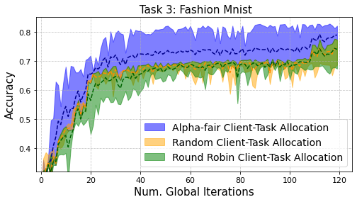
(b) Accuracy for task 3: Fashion-MNIST.

Figure 2: Results of Experiment 1: 3 tasks with varying difficulty levels. The 3 tasks have datasets MNIST, CIFAR-10, and Fashion-MNIST. FedFairMMFL achieves a higher minimum accuracy across tasks, as compared to the baselines, while maintaining the same or higher accuracy for the other 2 tasks (see Technical Report [36]).

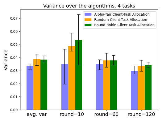
(a) Variance, Num. tasks=4.

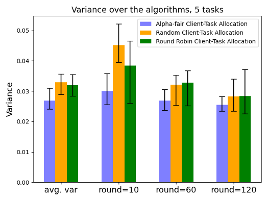
(b) Variance, Num. tasks=5.

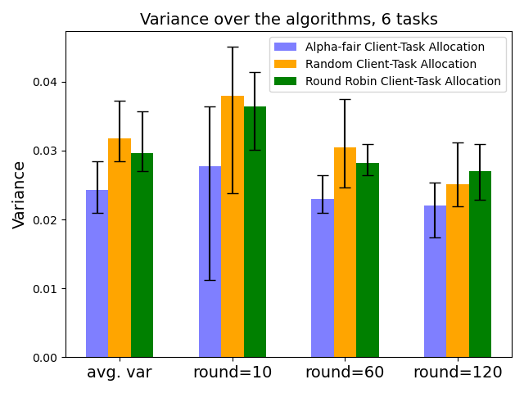
(c) Variance, Num. tasks=6.

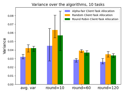
(d) Variance, Num. tasks=10.

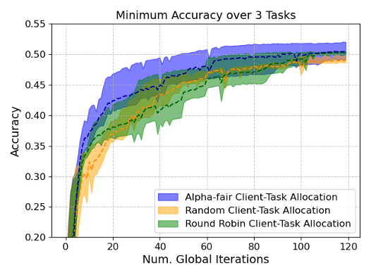
(e) Min accuracy, Num. tasks=3.

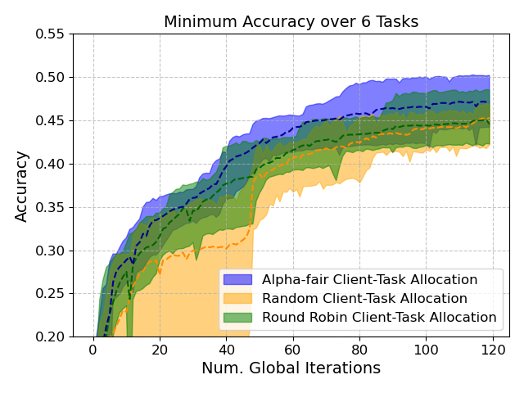
(f) Min accuracy, Num. tasks=6.

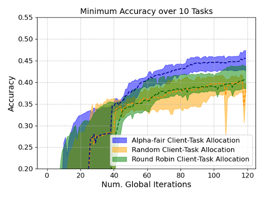
(g) Min accuracy, Num. tasks=10.

Figure 3: Results of Experiment 2: Increasing the number of tasks. (a), (b), (c), and (d) compare the variance in accuracy observed across multiple tasks, when employing the different algorithms. The error bars denote the max/min values of the corresponding variance among all 4 random seeds. Our algorithm generally achieves a lower variance amongst task performance. (e), (f), and (g) show the trend of minimum accuracy when task numbers are 3, 6, and 10, respectively.

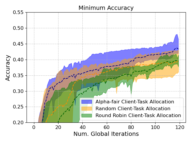
(a) Num. Clients=80.

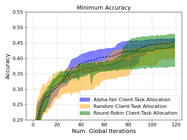
(b) Num. Clients=120.

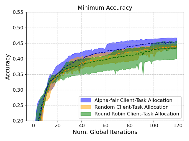
(c) Num. Clients=160.

Figure 4: Results of Experiment 3: Increasing the number of clients. All experiments have 5 tasks (MNIST, CIFAR-10, Fashion-MNIST, EMNIST, and CIFAR-10). Experiments are conducted with 4 random seeds. The participation rate is 0.25, and client numbers are 80, 120, and 160, respectively. Our algorithm FedFairMMFL generally achieves a higher minimum accuracy, and/or a faster convergence.

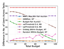
(a) Difference in the number of users which will train the tasks in MMFL.

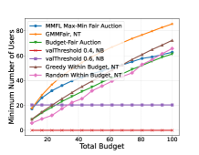
(b) Minimum number of users recruited for training, over two tasks.

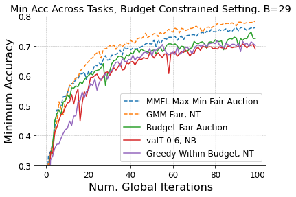
(c) The minimum accuracy after combining our auction strategies and baselines, with FedFairMMFL.

Figure 5: Results of Experiment 4: Client Take-Up Rates. (NB= No Budget, NT= Non Truthful Mechanism). Our near-truthful auction MMFL Max-Min Fair (a) leads to a lower difference in the number of users across tasks, and (b) incentivizes more clients than any incentivization algorithm but the un-truthful GMMFair. Results of Experiments 5: How auctions impact learning. Fig. (c) shows the minimum accuracy after combining the results of our auction strategies and baselines, with FedFairMMFL. The MMFL Max-Min Fair Auction leads to higher accuracies.

Finally we evaluate FedFairMMFL and our auction schemes. Our main results are that (i) FedFairMMFL consistently performs fairly across different experiment settings and (ii) our max-min auction increases the minimum learning accuracy across tasks in the budget constrained setting. We concurrently train (i) three tasks of varied difficulty levels, and evaluate the algorithms’ performance across varied numbers of (ii) tasks and (iii) clients. We analyze (iv) the impact of our auctions and baselines on the take-up rate over tasks, and analyze (v) the impact of these take-up rates on the tasks’ learning outcomes. We use $\alpha=3$ for FedFairMMFL in all experiments. The effect of different $\alpha$ is also measured (see Technical Report [36]).

Our client-task allocation algorithm FedFairMMFL is measured against two baselines: a) Random, where clients are randomly allocated a task with equal probability each global epoch (note that this corresponds to taking $\alpha=1$ in our $\alpha$-fair allocation), and b) Round Robin [8], where active clients are allocated to tasks in a round-robin manner, sequentially across global epochs. Our main fairness metrics are the minimum test accuracy across all tasks and the variance of the test accuracies (cf. Lemma 1). As some models may have larger training losses by nature, e.g., if they are defined on different datasets, making them more easily favored by the algorithm, we use the test accuracy instead of training loss in FedFairMMFL. Each experiment’s results are averaged over 3-5 random seeds - we plot the average values (dotted line), along with the maximum and minimum values indicated by the shaded area. Each client’s data is sampled from either all classes (i.i.d.) or a randomly chosen half of the classes (non-i.i.d.).

Experiment 1: Tasks of Varying Difficulty Levels. To model differing task difficulties, our tasks are to train image recognition models on MNIST and Fashion-MNIST on a convolutional neural network with 2 convolutional, 2 pooling, and 2 fully connected layers; and CIFAR-10 with a pre-activated ResNet. Experiments are run with 120 clients having $150-250$ datapoints from five (randomly chosen) of the ten classes (i.e., non i.i.d. data); $35\%$ of clients, chosen uniformly at random, are active each round. As seen in Fig. 2 a), FedFairMMFL has a higher minimum accuracy than the random and round robin baselines. FedFairMMFL adaptively allocates more clients to the prevailing worst-performing task, resulting in a higher accuracy for this task (Task 3: Fashion-MNIST), as seen in Fig. 2 b), while maintaining the same or a slightly higher accuracy for the other tasks (see Tech Report[36]). Though we might guess that CIFAR-10 would be the worst-performing task, as it uses the largest model, FedFairMMFL identifies that Fashion-MNIST is the worst-performing task, and it achieves fair convergence even in this challenging setting where Fashion-MNIST persistently performs worse than the other tasks.

Experiment 2: Increasing the number of tasks. To further understand the various algorithms (FedFairMMFL and the random allocation and round robin baselines) under different settings, their performance is measured as we increase the number of tasks, from 3 to 4, 5, 6 and 10. The tasks include MNIST, Fashion-MNIST, CIFAR-10, and EMNIST. We use the same networks as in Experiment 1 and a similar convolutional neural network with 2 convolutional, 2 pooling, and 2 fully connected layers for the EMNIST task. Experiments are run with 20 clients, having a participation rate of 1. Each client has $400-600$ datapoints from each dataset for each task. We plot the variance amongst tasks on average, as well as at global epoch round numbers 10, 60, and 120. As seen in Fig. 3, with the increase in the round number, all algorithms’ variance decreases, and FedFairMMFL has the lowest variance for all settings. This can be explained through the fact that FedFairMMFL dynamically allocates clients with a higher probability to tasks which are currently performing worse, eliminating the difference among tasks as training progresses. This effect remains even as we increase the number of tasks, which slows the training for all tasks as the clients are being shared among more tasks - see Fig. 3 (e), (f), and (g), which compare the minimum accuracy among different algorithms when task numbers are 3, 6, and 10. FedFairMMFL converges faster than both baselines.

Experiment 3: Increasing the number of clients. Different client numbers are also tested to further evaluate FedFairMMFL’s performance. Here, all experiments have 5 tasks (MNIST, CIFAR-10, Fashion-MNIST, EMNIST, and CIFAR-10), with client participation rate $25\%$ and $200-300$ datapoints for each client. We vary the number of clients from 80 to 160. Experiment results are shown in Fig. 4. It is clear to see that in this setting, FedFairMMFL outperforms the other two algorithms, either achieving a higher minimum accuracy, and/or a faster convergence. Its performance is also further improved as the client number increases, and is more stable among different random seeds, likely because having more clients allows the worse-performing tasks to ”catch up” with the others faster under the $\alpha$-fair allocation.

Experiment 4: Client Take-Up Rates. We compare the number of clients incentivized to train each task under our budget-fair (Section V-A) and max-min fair (Section V-B) auctions, as well as the (un-truthful) GMMFair algorithm, which upper-bounds the max-min fair auction result, and 4 other baselines: valThreshold 0.4 and valThreshold 0.6 assume no budget but that all users with cost (valuation) $c_{i,s}<0.4$ (respectively $c_{i,s}<0.6$) will agree to train the task; these simulate posted-price mechanisms that show the effect of the incentivization budget. Greedy Within Budget and Random Within Budget evenly divide the budget across tasks. Clients are added by ascending bid (for Greedy Within Budget) and randomly (for Random Within Budget), until the budget is consumed; comparison to these baselines shows the cost of enforcing truthfulness in the budget-fair auction. We consider two tasks and 100 clients; client bids are between 0 and 1 and are independently drawn from a truncated Gaussian distribution for Task 1 and an increasing linear distribution for Task 2. Results are averaged across 5 random seeds.

As seen in Fig. 5 a), our auction MMFL Max-min Fair leads to the lowest difference in the number of clients across tasks, managing to hit the theoretical optimal of the non-truthful algorithm GMMFair. Greedy within budget assigned the most clients to task 1, resulting in a high ”difference” as it assigns less clients to task 2 (increasing linear distribution of valuations), nevertheless Greedy within budget (along with GMMFair and Random within budget) are not truthful. Both Greedy within budget (non truthful) and the Budget-Fair Auction become more fair (decreasing difference across tasks) as the budget increases. Nevertheless MMFL Max-Min Fair outperforms them in the budget constrained region. As seen in Fig. 5 b), GMMFair yields the highest minimum number of users assigned to each task, consistent with Lemma 7. When the budget is low (budget constrained regime), our near-truthful auction MMFL Max-min Fair outperforms all the other mechanisms in the minimumn number of users. As the budget increases, the greedy-based mechanisms outperform it. Nevertheless, they and GMMFair are not truthful, and can be manipulated if all users jointly submit high bids.

Experiment 5: Take-Up Rates and Learning Outcomes. We finally consider a constrained budget ($B=29$) and evaluate how the outcome of the client recruitment strategies impact MMFL model training. Fig. 5 c) shows the minimum test accuracy across the two tasks (MNIST and CIFAR-10) at each training round, using FedFairMMFL for client-task allocation. GMMFair consistently has the highest minimum accuracy across tasks, likely because it recruits the most clients to each task, as shown in Experiment 4 (Fig. 5 b). Our MMFL auction, which additionally has the benefit of near-truthfulness, achieves nearly the same minimum accuracy, showing that it performs well in tandem with FedFairMMFL.

VII Conclusion and Future Directions

In this paper, we consider the fair training of concurrent MMFL tasks. Ours is the first work to both theoretically and experimentally validate algorithms that ensure fair outcomes across different learning tasks. We first propose FedFairMMFL, a simple algorithm to allocate clients to tasks in each training round, showing that it permits theoretical convergence guarantees. We then propose two auction mechanisms, Budget-Fair and MMFL Max-Min Fair, that seek to incentivize a fair number of clients to commit to training each task. Our experimental results for training different combinations of FL tasks show that FedFairMMFL and MMFL Max-Min Fair can jointly ensure fair convergence rates and final test accuracies across the different tasks. As the first work to consider fairness in the MMFL setting, we expect our work to seed many future directions, including how to balance achieving fairness over tasks with fairness over clients’ utilities. Another direction is to investigate fairness when tasks have differing difficulties and clients have heterogeneous, stochastic available computing resources for training each task.

References

- [1] B. McMahan, E. Moore, D. Ramage, S. Hampson, and B. A. y Arcas, “Communication-efficient learning of deep networks from decentralized data,” in Artificial intelligence and statistics. PMLR, 2017, pp. 1273–1282.
- [2] Y. Yao, M. M. Kamani, Z. Cheng, L. Chen, C. Joe-Wong, and T. Liu, “Fedrule: Federated rule recommendation system with graph neural networks,” in Accepted to ACM/IEEE IoTDI, 2023.
- [3] U. M. Aïvodji, S. Gambs, and A. Martin, “Iotfla: A secured and privacy-preserving smart home architecture implementing federated learning,” in 2019 IEEE security and privacy workshops. IEEE, 2019, pp. 175–180.
- [4] Y. Liu, L. Su, C. Joe-Wong, S. Ioannidis, E. Yeh, and M. Siew, “Cache-enabled federated learning systems,” in Proceedings of the Twenty-fourth International Symposium on Theory, Algorithmic Foundations, and Protocol Design for Mobile Networks and Mobile Computing, 2023, pp. 1–11.
- [5] D. C. Nguyen, Q.-V. Pham, P. N. Pathirana, M. Ding, A. Seneviratne, Z. Lin, O. Dobre, and W.-J. Hwang, “Federated learning for smart healthcare: A survey,” ACM Computing Surveys, vol. 55, no. 3, pp. 1–37, 2022.
- [6] A. Imteaj and M. H. Amini, “Distributed sensing using smart end-user devices: Pathway to federated learning for autonomous iot,” in 2019 International conference on computational science and computational intelligence (CSCI). IEEE, 2019, pp. 1156–1161.
- [7] N. Bhuyan, S. Moharir, and G. Joshi, “Multi-model federated learning with provable guarantees,” arXiv preprint arXiv:2207.04330, 2022.
- [8] N. Bhuyan and S. Moharir, “Multi-model federated learning,” in 2022 14th International Conference on COMmunication Systems & NETworkS (COMSNETS). IEEE, 2022, pp. 779–783.
- [9] C. Li, C. Li, Y. Zhao, B. Zhang, and C. Li, “An efficient multi-model training algorithm for federated learning,” in 2021 IEEE Global Communications Conference (GLOBECOM). IEEE, 2021, pp. 1–6.
- [10] Z.-L. Chang, S. Hosseinalipour, M. Chiang, and C. G. Brinton, “Asynchronous multi-model federated learning over wireless networks: Theory, modeling, and optimization,” arXiv preprint arXiv:2305.13503, 2023.
- [11] M. Siew, S. Arunasalam, Y. Ruan, Z. Zhu, L. Su, S. Ioannidis, E. Yeh, and C. Joe-Wong, “Fair training of multiple federated learning models on resource constrained network devices,” in Proceedings of the 22nd International Conference on Information Processing in Sensor Networks, 2023, pp. 330–331.
- [12] C. Joe-Wong, S. Sen, T. Lan, and M. Chiang, “Multiresource allocation: Fairness–efficiency tradeoffs in a unifying framework,” IEEE/ACM Transactions on Networking, vol. 21, no. 6, pp. 1785–1798, 2013.
- [13] E. Altman, K. Avrachenkov, and A. Garnaev, “Generalized -fair resource allocation in wireless networks,” in 2008 47th IEEE Conference on Decision and Control. IEEE, 2008, pp. 2414–2419.
- [14] E. Bampis, B. Escoffier, and S. Mladenovic, “Fair resource allocation over time,” in AAMAS 2018-17th International Conference on Autonomous Agents and MultiAgent Systems. International Foundation for Autonomous Agents and Multiagent Systems, 2018, pp. 766–773.
- [15] Y. Deng, F. Lyu, J. Ren, Y.-C. Chen, P. Yang, Y. Zhou, and Y. Zhang, “Fair: Quality-aware federated learning with precise user incentive and model aggregation,” in IEEE INFOCOM 2021-IEEE Conference on Computer Communications. IEEE, 2021, pp. 1–10.
- [16] T. Lan, D. Kao, M. Chiang, and A. Sabharwal, An axiomatic theory of fairness in network resource allocation. IEEE, 2010.
- [17] T. Li, M. Sanjabi, A. Beirami, and V. Smith, “Fair resource allocation in federated learning,” arXiv preprint arXiv:1905.10497, 2019.
- [18] Y. Zhang and Q. Yang, “A survey on multi-task learning,” IEEE Transactions on Knowledge and Data Engineering, vol. 34, no. 12, pp. 5586–5609, 2022.
- [19] Y. Ruan and C. Joe-Wong, “Fedsoft: Soft clustered federated learning with proximal local updating,” in Proceedings of the AAAI Conference on Artificial Intelligence, vol. 36, no. 7, 2022, pp. 8124–8131.
- [20] M. Hu, P. Zhou, Z. Yue, Z. Ling, Y. Huang, Y. Liu, and M. Chen, “Fedcross: Towards accurate federated learning via multi-model cross aggregation,” arXiv preprint arXiv:2210.08285, 2022.
- [21] W. Xia, T. Q. Quek, K. Guo, W. Wen, H. H. Yang, and H. Zhu, “Multi-armed bandit-based client scheduling for federated learning,” IEEE Transactions on Wireless Communications, vol. 19, no. 11, pp. 7108–7123, 2020.
- [22] Y. J. Cho, J. Wang, and G. Joshi, “Towards understanding biased client selection in federated learning,” in International Conference on Artificial Intelligence and Statistics. PMLR, 2022, pp. 10 351–10 375.
- [23] T. Nishio and R. Yonetani, “Client selection for federated learning with heterogeneous resources in mobile edge,” in 2019 IEEE international conference on communications (ICC). IEEE, 2019, pp. 1–7.
- [24] J. Liu, J. Jia, B. Ma, C. Zhou, J. Zhou, Y. Zhou, H. Dai, and D. Dou, “Multi-job intelligent scheduling with cross-device federated learning,” IEEE Transactions on Parallel and Distributed Systems, vol. 34, no. 2, pp. 535–551, 2022.
- [25] M. N. Nguyen, N. H. Tran, Y. K. Tun, Z. Han, and C. S. Hong, “Toward multiple federated learning services resource sharing in mobile edge networks,” IEEE Transactions on Mobile Computing, vol. 22, no. 1, pp. 541–555, 2021.
- [26] P. Poullie, T. Bocek, and B. Stiller, “A survey of the state-of-the-art in fair multi-resource allocations for data centers,” IEEE Transactions on Network and Service Management, vol. 15, no. 1, pp. 169–183, 2017.
- [27] A. Lakhdari and A. Bouguettaya, “Fairness-aware crowdsourcing of iot energy services,” in Service-Oriented Computing: 19th International Conference, ICSOC 2021, Virtual Event, November 22–25, 2021, Proceedings 19. Springer, 2021, pp. 351–367.
- [28] F. Basık, B. Gedik, H. Ferhatosmanoğlu, and K.-L. Wu, “Fair task allocation in crowdsourced delivery,” IEEE Transactions on Services Computing, vol. 14, no. 4, pp. 1040–1053, 2018.
- [29] X. Gan, Y. Li, W. Wang, L. Fu, and X. Wang, “Social crowdsourcing to friends: An incentive mechanism for multi-resource sharing,” IEEE Journal on Selected Areas in Communications, vol. 35, no. 3, pp. 795–808, 2017.
- [30] K. Donahue and J. Kleinberg, “Models of fairness in federated learning,” arXiv preprint arXiv:2112.00818, 2021.
- [31] Y. Zhan, J. Zhang, Z. Hong, L. Wu, P. Li, and S. Guo, “A survey of incentive mechanism design for federated learning,” IEEE Transactions on Emerging Topics in Computing, vol. 10, no. 2, pp. 1035–1044, 2021.
- [32] Y. Zhan, P. Li, Z. Qu, D. Zeng, and S. Guo, “A learning-based incentive mechanism for federated learning,” IEEE Internet of Things Journal, vol. 7, no. 7, pp. 6360–6368, 2020.
- [33] J. Weng, J. Weng, H. Huang, C. Cai, and C. Wang, “Fedserving: A federated prediction serving framework based on incentive mechanism,” in IEEE INFOCOM 2021. IEEE, 2021, pp. 1–10.
- [34] X. Wang, S. Zheng, and L. Duan, “Dynamic pricing for client recruitment in federated learning,” arXiv preprint arXiv:2203.03192, 2022.
- [35] M. Tang and V. W. Wong, “An incentive mechanism for cross-silo federated learning: A public goods perspective,” in IEEE Conference on Computer Communications. IEEE, 2021, pp. 1–10.
- [36] “Technical report.” [Online]. Available: http://tinyurl.com/MMFLpaper
- [37] Y. Ruan, X. Zhang, and C. Joe-Wong, “How valuable is your data? optimizing client recruitment in federated learning,” in 2021 19th International Symposium on Modeling and Optimization in Mobile, Ad hoc, and Wireless Networks (WiOpt). IEEE, 2021, pp. 1–8.
- [38] Y. Singer, “Budget feasible mechanism design,” ACM SIGecom Exchanges, vol. 12, no. 2, pp. 24–31, 2014.