Waiting time statistics for a double quantum dot coupled with an optical cavity

Abstract

A double quantum dot coupled to an optical cavity is a prototypical example of a non-trivial open quantum system. Recent experimental and theoretical studies show that this system is a candidate for single-photon detection in the microwave domain. This motivates studies that go beyond just the average current, and also take into account the full counting statistics of photon and electron detections. With this in mind, here we provide a detailed analysis of the waiting time statistics of this system within the quantum jump unravelling, which allows us to extract analytical expressions for the success and failure probabilities, as well as for the inter-detection times. Furthermore, by comparing single and multi-photon scenarios, we infer a hierarchy of occurrence probabilities for the different events, highlighting the role of photon interference events in the detection probabilities. Our results therefore provide a direct illustration of how waiting time statistics can be used to optimize a timely and relevant metrological task.

I Introduction

The utilization of waiting time statistics formalism extends to the analysis of diverse stochastic processes, encompassing realms such as quantum optics Vyas and Singh (1988); Carmichael et al. (1989), electronic transport Haack et al. (2014); Thomas and Flindt (2013), and entropy production estimation Skinner and Dunkel (2021), as pioneered by Stratonovich Stratonovich (1967). This powerful tool finds application in quantum master equations, enabling the study of system dynamics through quantum jumps, shifting the focus from explicit solutions of the von Neumann equation to the examination of waiting time distributions (WTDs) Brandes (2008); Landi et al. (2023). Notably, this approach proves valuable when describing systems with discrete phenomena, such as the punctual creation or annihilation of modes, as is the case with the coupling of a double quantum dot (DQD) to an optical cavity (CO).

The theoretical framework of the DQD-CO coupling is intricate, representing a nontrivial fermionic system interacting with a nontrivial bosonic system, allowing for analytical solutions only under specific considerations Zenelaj et al. (2022). These solutions unveil the statistical nature and constraints of the system Zenelaj et al. (2022); Xu and Vavilov (2013); Wong and Vavilov (2017); Ghirri et al. (2020). Beyond its theoretical richness, the DQD-CO system holds direct experimental relevance in diverse fields, including spectroscopy Oosterkamp et al. (1998); Michalet et al. (2007), photon observation in astronomy Huber et al. (2013), the implementation of quantum circuits Nian et al. (2023), and emerging THz quantum technologies Todorov et al. (2024). Notably, the system’s distinctive feature lies in its ability to function as a photodetector with a unique characteristic: the capacity to capture microwave-scale photons, an energy range four to five times smaller than the optical regime Khan et al. (2021).

By employing the WTDs formalism, the analysis of the DQD-CO system enables the explicit determination of the probabilities associated with the success or failure of photon detection. Additionally, this approach complements the estimation of quantum efficiency through full counting statistics Zenelaj et al. (2022); Xu and Vavilov (2013), offering valuable insights into the performance of this system in photon detection applications.

In this paper we investigate the waiting time statistics of a DQD-OC setup, unraveled in terms of clicks associated to both electron detection and photon leaks. We focus on regimes allowing for analytical solutions, and show that these can shed light on the potential applications of these devices as single-photon detectors.

II System and Model

Our focus lies in the investigation of a system comprising a double quantum dot (DQD) coupled with an optical cavity (OC) Khan et al. (2021); Xu and Vavilov (2013), as depicted in Figure 1. The DQD can be conceptualized as two fermionic reservoirs (leads), each coupled to a potential well capable of accommodating a single fermion at any given moment. Within the Coulomb blockade regime, disregarding electron spin and focusing solely on its presence in the potential wells, the Hamiltonian describing the DQD is given by

$$H_{DQD}=\frac{\epsilon}{2}\left(\ket{R}\bra{R}-\ket{L}\bra{L}\right)+t_{c}\left(\ket{R}\bra{L}+\ket{L}\bra{R}\right),$$ (1)

where $\ket{0}$ represents the Fock state denoting the absence of electrons ($Z=0$), the presence of an electron in the right dot ($Z=R$), or in the left dot ($Z=L$). Here, $\epsilon$ signifies the energy of the dots, and $t_{c}$ represents the coupling energy between them. Employing a transformation matrix

$$\begin{pmatrix}\ket{L}\\ \ket{R}\\ \ket{0}\end{pmatrix}=\begin{pmatrix}-\frac{\epsilon}{\Omega}&\frac{2t_{c}}{\Omega}&0\\ -\frac{2t_{c}}{\Omega}&-\frac{\epsilon}{\Omega}&0\\ 0&0&1\end{pmatrix}\begin{pmatrix}\ket{g}\\ \ket{e}\\ \ket{0}\end{pmatrix},\quad\Omega\equiv\sqrt{4t_{c}^{2}+\epsilon^{2}},$$ (2)

we redefine $H_{DQD}$ in terms of the excited ($\ket{e}$) and ground ($\ket{g}$) eigenstates, yielding

$$H_{DQD}=\frac{\Omega}{2}\left(\ket{e}\bra{e}-\ket{g}\bra{g}\right)\equiv\frac{\Omega}{2}\sigma_{z}.$$ (3)

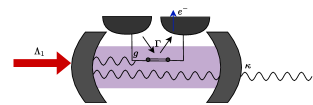
Figure 1: Double quantum dot coupled with an optical cavity.

Simultaneously, the OC is envisioned as the combination of a photon pump (e.g., LASER) with a geometric entity that predominantly selects photons possessing a specific frequency of interest Roberts and Clerk (2020). The total Hamiltonian $H_{OC}$ for this system is expressed as

$$H_{OC}=\omega_{r}a^{\dagger}a+\xi\left(e^{i\omega_{l}}a^{\dagger}+e^{-i\omega_{l}t}a\right),$$ (4)

where $a$ is a bosonic mode, $\omega_{r}$ denotes the resonance frequency of the cavity, $\omega_{l}$ is the pump frequency and $\xi$ is the pump strength.

Finally, to lowest order the DQD-OC coupling takes the form Khan et al. (2021)

$$H_{I}=g\left(a^{\dagger}\sigma_{-}+a\sigma_{+}\right),$$ (5)

where $\sigma_{+}\equiv\ket{e}\bra{g}$ is the raising operator for the DQD and $\sigma_{-}\equiv\sigma_{+}^{\dagger}$.

The unitary dynamics of the DQD-OC system, expressed by a Hamiltonian $H$ comprising (3), (4), and (5), is given in the rotating frame at the pump frequency, as Zenelaj et al. (2022)

$$H=\Delta_{d}\frac{\sigma_{3}}{2}+\Delta_{r}a^{\dagger}a+g\left(a^{\dagger}\sigma_{-}+a\sigma_{+}\right)+\xi\left(a^{\dagger}+a\right),$$ (6)

with $\Delta_{d}\equiv\Omega-\omega_{l}$ ($\Delta_{r}\equiv\omega_{r}-\omega_{l}$) representing the difference between the frequency of the DQD (OC) and the frequency of the pump.

Given the weak coupling in the DQD-OC system, the nonunitary dynamics can be modeled using independent dissipators for the DQD and OC  Breuer et al. (2002); Santos and Landi (2016). Specifically, focusing on single-photon dissipation, $\kappa\mathcal{D}[a]$ becomes the sole dissipator for the open dynamics of the OC, where $\kappa$ quantifies the dissipation rate and $\mathcal{D}[a]\rho=a\rho a^{\dagger}-\frac{1}{2}\{a^{\dagger}a,\rho\}$. In the case of the DQD, the ideal photodetector regime Zenelaj et al. (2022); Khan et al. (2021) is adopted, with interest centered on the input of electrons in the ground state (i.e., $\ket{0}\rightarrow\ket{g}$) and the output of electrons in the excited state (i.e., $\ket{e}\rightarrow\ket{0}$), both occurring at the same rate $\Gamma$. This is captured by $\Gamma\mathcal{D}[s_{g}^{\dagger}]$ and $\Gamma\mathcal{D}[s_{e}]$, respectively, with $s_{j}\equiv\ket{0}\bra{j}$ ($j=g,e$) representing the extraction of an electron in either the ground or excited states.

Consequently, the state $\rho$ governing the DQD-CO system is assumed to follow the Lindblad equation for its open dynamics

$$\dot{\rho}=-i\left[H,\rho\right]+\Gamma\mathcal{D}[s_{g}^{\dagger}]\rho+\Gamma\mathcal{D}[s_{e}]\rho+\kappa\mathcal{D}[a]\rho,$$ (7)

where $H$ is given by equation (6).

III Waiting Time Statistics

Prior to delving into the evaluation of pertinent quantities for DQD-CO system, it is instructive to introduce fundamental concepts of waiting time formalism Landi et al. (2023); Brandes (2008). The Lindblad equation (7) is recast as

$$\dot{\rho}=\mathcal{L}(\rho),$$ (8)

where $\mathcal{L}(\rho)$, given by the right side of (7), stands as the Liouvilian operator of the model. This formulation enables the expression of a formal solution

$$\rho(t)=e^{\mathcal{L}t}\rho(0),$$ (9)

which can be expanded in Dyson’s series as

$$\rho(t)=e^{\mathcal{L}0t}\rho(0)+\sum_{k\in\mathcal{M}}\int_{0}^{t}dt_{1}e^{\mathcal{L}_{0}(t-t_{1})}\mathcal{L}_{k}e^{\mathcal{L}0t_{1}}\rho(0)+\$$

$$+\sum_{k,q\in\mathcal{M}}\int_{0}^{t}dt_{2}\int_{0}^{t_{2}}dt_{1}e^{\mathcal{L}_{0}(t-t_{2})}\mathcal{L}_{k}e^{\mathcal{L}_{0}(t_{2}-t_{1})}\mathcal{L}_{q}e^{\mathcal{L}_{0}t_{1}}\rho(0)+...,$$ (10)

where

$$\mathcal{L}_{j}(\rho)=L_{j}\rho L_{j}^{\dagger},$$ (11)

represents the jumps observable in the system, and

$$\mathcal{L}0\equiv\mathcal{L}-\sum_{j\in\mathcal{M}}\mathcal{L}_{j}$$ (12)

is the no-jump operator. Here we also introduce the set $\mathcal{M}$ representing the jump operators which we assume can be monitored.

Each term in the expansion (10) corresponds to the probability associated with a specific number of jumps in the system. Notably, the probability of a jump occurring in the $j$-th channel at any given time is defined as a Waiting Time Distribution (WTD), expressed as

$$W(j,t|\rho)=\Tr{\mathcal{L}_{j}e^{\mathcal{L}_{0}t}\rho}.$$ (13)

Marginalizing over $t$, and assuming that the initial state is such that a jump must necessarily occur, yields

$$W(j|\rho)=\Tr{\mathcal{L}_{j}\left(\int_{0}^{\infty}dte^{\mathcal{L}_{0}t}\right)\rho}=-\Tr{\mathcal{L}_{j}\mathcal{L}_{0}^{-1}\rho},$$ (14)

which quantifies the likelihood of a jump in channel $j$, given that the initial state was $\rho$. Conversely, marginalizing over $j$ yields

$$W(t|\rho)=-\Tr\{\mathcal{L}_{0}e^{\mathcal{L}_{0}t}\rho\big{\}},$$ (15)

which is the probability distribution that the first jump occurs at time $t$, irrespective of in which channel it happens.

Similarly, for scenarios involving two jumps—one at time $t_{1}$ in channel $j_{1}$ and another at time $t_{2}$ in channel $j_{2}$—the associated probability distribution is given by

$$W\left(j_{1},t_{1},t_{2},j_{2}|\rho\right)=\Tr{\mathcal{L}_{j_{2}}e^{\mathcal{L}_{0}t_{2}}\mathcal{L}{j_{1}}e^{\mathcal{L}_{0}t_{1}}\rho}.$$ (16)

Furthermore, these distributions can be employed to define an average time for an event to occur in the system:

$$\langle t\rangle=\int_{0}^{\infty}dtW(t|\rho)t=-\Tr{\mathcal{L}_{0}^{-1}\rho}.$$ (17)

This quantity holds significance as it characterizes the characteristic time of the system’s evolution, playing a pivotal role in defining quasi-static processes in Thermodynamics Deffner and Campbell (2019).

IV Waiting Time Statistics of the DQD-OC system

The objective of this study is to formulate the probability distributions of success and failure in the detection of a photocurrent, given the presence of a photon within the cavity. The failure process is associated with photon leakage, while the success process is correlated with photon absorption by an electron. To address this problem analytically, we employ the ideal photodetector regime, assuming a weak pump ($\xi\ll 1$). The weak pump approximation is introduced by envisioning the activation of the pump, followed by a waiting period until the cavity absorbs $n$ photons. Due to the weak pump, the photon count remains nearly constant during this interval. Consequently, we can analyze the system’s dynamics within this time frame, treating the pump as negligible by setting $\xi=0$ and establishing an initial condition in the density matrix representing the $n$ initial photons in the cavity. We denote different choices of initial conditions as the ”$n$ photon scenario”, specified by the initial density matrix

$$\rho_{0}^{(n)}=\ket{\psi_{n}}\bra{\psi_{n}},\quad\ket{\psi_{n}}\equiv\ket{0}\otimes\ket{n}$$ (18)

where $\ket{n}$ is the Fock state of $n$ photons.

In the first step toward building a waiting time distribution, we identify the channels we can monitor—specifically, both the electron detection ($s_{e}$) and photon leakage channels ($a$). The channels of interest are the photocurrent channel (right reservoir in Figure 1) and the photon leak channel (photon accompanied by $\kappa$ in the same figure). The photocurrent channel can be represented by

$$\mathcal{L}_{e}\rho\equiv\Gamma s_{e}\rho s_{e}^{\dagger},$$ (19)

with jumps $\ket{e}\rightarrow\ket{0}$ in DQD, occurring at a rate of $\Gamma$. The photon leak channel is modeled by

$$\mathcal{L}_{\gamma}\rho\equiv\kappa a\rho a^{\dagger},$$ (20)

resulting in photon leakage from the cavity to the environment at a rate of $\kappa$.

Utilizing (19) and (20), we define a no-jump Liouvillian, implicitly determining the channels we lack access to:

$$\mathcal{L}_{0}=\mathcal{L}-\kappa\mathcal{L}_{\gamma}-\Gamma\mathcal{L}_{e}$$ (21)

This no-jump Liouvillian is employed to evaluate the probabilities of interest in a given scenario.

One Photon Scenario

We first consider the case $n=1$. In this scenario, two probabilities are of interest: the probability $p_{\gamma}$ of a single photon leaking to the environment and the probability $p_{e}$ of this photon being absorbed by an electron, resulting in a photocurrent. These probabilities are evaluated using Eq. (14), i.e.,

$$p_{j}\equiv W\left(j|\rho\right)=-\Tr{\mathcal{L}_{j}\mathcal{L}_{0}^{-1}\rho_{0}^{(1)}}.$$ (22)

The assumption that we start with a single photon in the cavity allows us to truncate the bosonic Hilbert space, and therefore obtain the following analytical expression for the success probability:

$$p_{e}=\frac{C}{C+1}\frac{\alpha^{2}}{(\alpha+1)^{2}},$$ (23)

where $C\equiv 4g^{2}/(\Gamma\kappa)$ is the cooperativity Aspelmeyer et al. (2014); Haroche and Raimond (2006) and $\alpha\equiv\Gamma/\kappa$ quantifies the competition between the electronic and bosonic dissipation rates. The failure probability is $p_{\gamma}=1-p_{e}$.

Notably, as $C\rightarrow 0$ or $\alpha\rightarrow 0$, $p_{e}\rightarrow 0$, or equivalently, $p_{\gamma}\rightarrow 1$. This is expected, as $\alpha\rightarrow 0$ implies more intense interaction of bosonic modes with the environment than fermionic modes, while $C\rightarrow 0$ indicates weak interaction between DQD and OC compared to their individual interactions with the environment. In both cases, photon absorption by an electron is attenuated. Conversely, $\alpha,C\gg 1$ implies $p_{e}\approx 1$, which is reasonable.

Furthermore, we evaluate the (dimensionless) average time $\kappa\langle t\rangle$ for any of the jumps ($e$ or $\gamma$) to occur in the system, representing the time until an event takes place (eq. 17), namely

$$\kappa\langle t\rangle=-\kappa\Tr{\mathcal{L}_{0}^{-1}\rho_{0}^{(1)}}=\frac{(\alpha+1)^{2}+C(3\alpha+1)}{(\alpha+1)^{2}(C+1)}.$$ (24)

Figure 5 illustrates the behavior of $\langle t\rangle$ in terms of $C$ for three distinct values of $\alpha$. For $0<\alpha<1$, the average time to an event increases with $C$, implying that the system takes longer to transition, within an upper bound given by $\kappa\langle t\rangle<(3\alpha+1)/(\alpha+1)^{2}$. Interestingly, we see that if $\alpha=1$ (equal dissipation rates for the two channels) we get $\kappa\langle t\rangle=1$, independent of the cooperativity. Notice that this is not true for $p_{e},p_{\gamma}$.

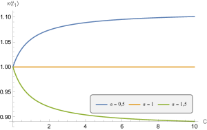
Figure 2: Average time.

Two Photon Scenario

Next we consider $n=2$. In this scenario, four probabilities of interest emerge instead of two: (i) the probability $p_{ee}$ of both initial photons being sequentially absorbed, resulting in a photocurrent; (ii) the probability $p_{e\gamma}$ of the first photon being absorbed and the second leaking; (iii) the probability of the first photon leaking, but the second being absorbed; and (iv) the probability $p_{\gamma\gamma}$ of both photons sequentially leaking. These two-sequential-jump probabilities are defined as (see eq. 16)

$$p_{ij}\equiv W(j,i|\rho)=\Tr{\mathcal{L}_{j}\mathcal{L}_{0}^{-1}\mathcal{L}_{i}\mathcal{L}_{0}^{-1}\rho_{0}^{(2)}},$$ (25)

with $i,j=e,\gamma$. We now find:

$$p_{ee} =\frac{C^{2}\alpha^{5}}{(1+C)(1+\alpha)^{2}(1+\alpha+C\alpha)(6+5\alpha+\alpha^{2})},$$ (26)

$$p_{e\gamma} =\frac{C\alpha^{3}\left(C+2C\alpha+(1+\alpha^{2})\right)}{(1+C)(1+\alpha)^{2}(3+\alpha)(1+\alpha+C\alpha)},$$ (27)

$$p_{\gamma e} =\frac{C\alpha^{2}\left(12+\alpha(3+\alpha)(7+\alpha)+C\alpha(9+5\alpha)\right)}{(1+C)(1+\alpha)^{2}(3+\alpha)(1+\alpha+C\alpha)},$$ (28)

$$p_{\gamma\gamma} =1-p_{ee}-p_{e\gamma}-p_{\gamma e}$$ (29)

We can further idetity probabilities allow us to identify

$$p_{e1}\equiv p_{ee}+p_{e\gamma}=\frac{C\alpha^{3}}{(2+\alpha)(3+\alpha)(1+\alpha+C\alpha)}$$ (30)

and

$$p_{e2} \equiv p_{ee}+p_{\gamma e}$$ (31)

$$=\frac{C\alpha^{2}\left(12+3(7+3C)\alpha+5(2+C)\alpha^{2}+(1+C)\alpha^{3}\right)}{(1+C)(1+\alpha)^{2}(2+\alpha)(3+\alpha)(1+\alpha+C\alpha)}$$ (32)

as the probability of a jump occurring in the $e$-channel (i.e., detection of a photocurrent) in the first and second measurements, respectively. These quantities, along with $p_{ee}$ (eq. 26) and $p_{e}$ (eq. 23), are plotted in Figure 3, where the hierarchy

$$p_{e2}\geq p_{e}\geq p_{e1},\quad\forall\text{ }\alpha,C,$$ (33)

is observed. Eq. (33) indicates that the probability of detecting a photocurrent in the first measurement in the two-photon scenario is lower than in the one-photon scenario, while the opposite holds for the probability of the second measurement resulting in a photocurrent, as it is always greater than the others. This result, independent of $\alpha$ and $C$, provides a method for verifying the scenario and highlights the nontrivial interference effects when there are multiple photons inside the cavity.

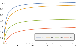
Figure 3: Photocurrent hierarchy.

The asymptotic limits $\alpha\rightarrow\infty$ and $C\rightarrow\infty$ yield

$$\lim_{\alpha\rightarrow\infty}p_{ee}=\frac{C^{2}}{(1+C)^{2}},$$ (34)

and

$$\lim_{\alpha\rightarrow\infty}p_{e\gamma}=\lim_{\alpha\rightarrow\infty}p_{\gamma e}=\lim_{\alpha\rightarrow\infty}p_{e}=\frac{C}{(1+C)^{2}},$$ (35)

in which we recalled equation (23). This last result indicates that in the strong fermionic interaction regime, the two-photon scenario reduces to a pair of one-photon scenarios, rendering them indistinguishable. However, the same is not true for the large cooperativity regime, where

$$\lim_{C\rightarrow\infty}p_{ee}=\frac{\alpha^{4}}{(1+\alpha)^{2}(6+5\alpha+\alpha^{2})},$$ (36)

$$\lim_{C\rightarrow\infty}p_{e\gamma}=\frac{\alpha^{2}(1+2\alpha)}{(1+\alpha)^{2}(6+5\alpha+\alpha^{2})},$$ (37)

and

$$\lim_{C\rightarrow\infty}p_{\gamma e}=\frac{\alpha^{2}(9+5\alpha)}{(1+\alpha)^{2}(6+5\alpha+\alpha^{2})}.$$ (38)

In this case, a nontrivial dependence on $\alpha$ exists in all cases, preventing specific conclusions. This observation underscores $\alpha$ as the parameter characterizing the scenarios. Finally, it is worth noting that

$$\lim_{\alpha\rightarrow 0}p_{ij}=\lim_{C\rightarrow 0}p_{ij}=\delta_{i\gamma}\delta_{\gamma j},$$ (39)

which is expected, as previously discussed in the one-photon scenario.

V Concluding Remarks

In conclusion, under the assumption of a weak-pump regime, we have leveraged the formalism of waiting statistics to derive probabilities governing the success and failure of photocurrent conversion within a DQD-CO system, examining scenarios involving one and two incident photons. While the extension of this approach to scenarios involving $n$ photons is conceptually straightforward, it is imperative to note that the validity of this approximation diminishes as $n$ increases, as it fails to account for mixed states at its core, leading to nonphysical outcomes.

Nevertheless, our methodology adequately captures the interference effects between photons within the cavity, significantly influencing the photocurrent detection process. A logical progression involves constructing WTDs for non-zero detunings ($\xi\neq 0$), corresponding to scenarios with reasonable to strong pumping. This analysis is anticipated to shed light on how the probabilities of photocurrent conversion evolve with varying pump intensities.

Moreover, we envisage incorporating additional complexities into our model, such as losses through phononic channels, as outlined in the work by Zenelaj et al. Zenelaj et al. (2022). This enhancement will contribute to a more realistic representation of the DQD-CO system, accounting for factors beyond the weak-pump approximation and further refining our understanding of the underlying physical processes.

References

- Vyas and Singh (1988) R. Vyas and S. Singh, Physical Review A 38, 2423 (1988).
- Carmichael et al. (1989) H. Carmichael, S. Singh, R. Vyas, and P. Rice, Physical Review A 39, 1200 (1989).
- Haack et al. (2014) G. Haack, M. Albert, and C. Flindt, Physical Review B 90, 205429 (2014).
- Thomas and Flindt (2013) K. H. Thomas and C. Flindt, Physical Review B 87, 121405 (2013).
- Skinner and Dunkel (2021) D. J. Skinner and J. Dunkel, Physical review letters 127, 198101 (2021).
- Stratonovich (1967) R. L. Stratonovich, Topics in the theory of random noise, Vol. 2 (CRC Press, 1967).
- Brandes (2008) T. Brandes, Annalen der Physik 520, 477 (2008).
- Landi et al. (2023) G. T. Landi, M. J. Kewming, M. T. Mitchison, and P. P. Potts, arXiv preprint arXiv:2303.04270 (2023).
- Zenelaj et al. (2022) D. Zenelaj, P. P. Potts, and P. Samuelsson, Physical Review B 106, 205135 (2022).
- Xu and Vavilov (2013) C. Xu and M. G. Vavilov, Physical Review B 88, 195307 (2013).
- Wong and Vavilov (2017) C. H. Wong and M. G. Vavilov, Physical Review A 95, 012325 (2017).
- Ghirri et al. (2020) A. Ghirri, S. Cornia, and M. Affronte, Sensors 20, 4010 (2020).
- Oosterkamp et al. (1998) T. Oosterkamp, T. Fujisawa, W. Van Der Wiel, K. Ishibashi, R. Hijman, S. Tarucha, and L. P. Kouwenhoven, Nature 395, 873 (1998).
- Michalet et al. (2007) X. Michalet, O. Siegmund, J. Vallerga, P. Jelinsky, J. Millaud, and S. Weiss, Journal of modern optics 54, 239 (2007).
- Huber et al. (2013) M. C. Huber, A. Pauluhn, and J. G. Timothy, in Observing Photons in Space: A Guide to Experimental Space Astronomy (Springer, 2013) pp. 1–19.
- Nian et al. (2023) L.-L. Nian, S. Hu, L. Xiong, J.-T. Lü, and B. Zheng, Physical Review B 108, 085430 (2023).
- Todorov et al. (2024) Y. Todorov, S. Dhillon, and J. Mangeney, Nanophotonics (2024).
- Khan et al. (2021) W. Khan, P. P. Potts, S. Lehmann, C. Thelander, K. A. Dick, P. Samuelsson, and V. F. Maisi, Nature communications 12, 5130 (2021).
- Roberts and Clerk (2020) D. Roberts and A. A. Clerk, Physical Review X 10, 021022 (2020).
- Breuer et al. (2002) H.-P. Breuer, F. Petruccione, et al., The theory of open quantum systems (Oxford University Press on Demand, 2002).
- Santos and Landi (2016) J. P. Santos and G. T. Landi, Physical Review E 94, 062143 (2016).
- Deffner and Campbell (2019) S. Deffner and S. Campbell, Quantum Thermodynamics: An introduction to the thermodynamics of quantum information (Morgan & Claypool Publishers, 2019).
- Aspelmeyer et al. (2014) M. Aspelmeyer, T. J. Kippenberg, and F. Marquardt, Reviews of Modern Physics 86, 1391 (2014).
- Haroche and Raimond (2006) S. Haroche and J.-M. Raimond, Exploring the quantum: atoms, cavities, and photons (Oxford university press, 2006).