TOI-837 b is a Young Saturn-sized Exoplanet with a Massive 70 Core
Abstract
We present an exhaustive photometric and spectroscopic analysis of TOI-837, a F9/G0 35 Myr young star, hosting a transiting exoplanet, TOI-837 b, with an orbital period of 8.32 d. Utilising data from TESS and ground-based observations, we determine a planetary radius of 0.82 for TOI-837 b. Through detailed HARPS spectroscopic time series analysis, we derive a Doppler semi-amplitude of 36 , corresponding to a planetary mass of 0.39 . The derived planetary properties suggest a substantial core of approximately 70 , constituting about 60% of the planet’s total mass. This finding poses a significant challenge to existing theoretical models of core formation. We propose that future atmospheric observations with JWST could provide insights into resolving ambiguities of TOI-837 b, offering new perspectives on its composition, formation, and evolution.
keywords:
Planets and satellites: individual: TOI-837 – Stars: activity – Techniques: radial velocities – Techniques: photometric1 Introduction
Characterising the properties of young exoplanets ( Gyr) at different stages is crucial to understanding the evolution and populations of exoplanets. These planets are often elusive to detection using indirect techniques like transit and radial velocity (RV) methods, as strong stellar activity generates stellar signals that often overshadows their signals in photometric and spectroscopic data. Recently, tens of young transiting exoplanets have been discovered (e.g., Bouma et al., 2020; David et al., 2018; Hobson et al., 2021; Martioli et al., 2021; Mann et al., 2021; Rizzuto et al., 2020; Barragán et al., 2022b). This success is largely attributed to missions like K2 (Howell et al., 2014) and the Transiting Exoplanet Survey Satellite (TESS; Ricker et al., 2015) that provide thousands of light curves of young stars.
After identifying a young transiting exoplanet, the next step typically involves spectroscopic observations to observe the star’s RV variations caused by the planet to measure its mass. However, separating signals from the planet and star in radial velocity data remains challenging. Gaussian Processes (GPs) have emerged as a favoured method for modelling activity-induced radial velocities, offering a flexible way to represent stochastic variations, such as the quasi-periodic stellar signals (see e.g., Aigrain & Foreman-Mackey, 2023). Multiple authors have used GPs, and variations of them such as multidimensional GPs (see e.g., Rajpaul et al., 2015; Barragán et al., 2022a), to detect RV planetary signals on spectroscopic time series of active young stars (e.g., Barragán et al., 2019b, 2023; Mantovan et al., 2023; Mallorquín et al., 2023; Zicher et al., 2022). Nevertheless, although widely embraced by the community, there exists a notable concern that the GP activity model may inadvertently mask or alter potential planetary signals (see e.g., discussions in Ahrer et al., 2021; Rajpaul et al., 2021). A recent example of this comes from Suárez Mascareño et al. (2021). The authors, utilising GPs, discovered that the planets orbiting the young V 1298 Tau exhibited significantly higher density than anticipated. However, these detections have been challenged by the exoplanet community. Blunt et al. (2023) suggested that Suárez Mascareño et al. (2021)’s detections may have been affected by over-fitting, thereby questioning the reliability of their RV Doppler detections. This is crucial, especially in cases where the measurements are in tension with models.
Bouma et al. (2020, hereafter B20) reported the discovery and validation of the young transiting exoplanet around TOI-837. The star is a young () F9/G0 dwarf star in the southern open cluster IC 2602. TOI-837’s main identifiers and parameters are given in Table 1. They used TESS cycle 1, the GAIA mission, multi-band photometry and spectroscopic observations to validate the planetary nature of a transit signal. The transit object corresponds to a planet with a radius of and a period of d. In this manuscript, we present a spectroscopic follow-up and exhaustive analysis of TOI-837, to characterise further the nature of TOI-837 b. This paper is structured as follows: The photometric and spectroscopic data of TOI-837 are detailed in Section 2. The analytical methods applied to this data are outlined in Section 3. A discussion of the findings is provided in Section 4, and the paper concludes with a summary of the key outcomes in Section 5. This manuscript is part of a series of papers under the project GPRV: Overcoming stellar activity in radial velocity planet searches funded by the European Research Council (ERC, P.I. S. Aigrain).
| Parameter | Value | Source |
| Main identifiers | ||
| Gaia DR3 | 5251470948229949568 | Gaia Collaboration (2020) |
| TYC | 8964-17-1 | Høg et al. (2000) |
| 2MASS | J10280898-6430189 | Cutri et al. (2003) |
| Spectral type | F9/G0 | Bouma et al. (2020) |
| Equatorial coordinates, proper motion, and parallax | ||
| (J2000.0) | 10 28 08.9903 | Gaia Collaboration (2020) |
| (J2000.0) | -64 30 18.9364 | Gaia Collaboration (2020) |
| (mas ) | Gaia Collaboration (2020) | |
| (mas ) | Gaia Collaboration (2020) | |
| (mas) | Gaia Collaboration (2020) | |
| Distance (pc) | Gaia Collaboration (2020) | |
| Magnitudes | ||
| B | Høg et al. (2000) | |
| V | Høg et al. (2000) | |
| Gaia | Gaia Collaboration (2020) | |
| J | Cutri et al. (2003) | |
| H | Cutri et al. (2003) | |
| Ks | Cutri et al. (2003) | |
| W1 | AllWISE | |
| W2 | AllWISE | |
| W3 | AllWISE | |
| Stellar parameters | ||
| (K) | This work | |
| spec (cgs) | This work | |
| [Fe/H] | This work | |
| () | This work | |
| Mass (M⊙) | This work | |
| Radius (R⊙) | This work | |
| Luminosity (L⊙) | This work | |
| Density () | This work | |
| isoc (cgs) | This work | |
| Age (Myr) | This work | |
| (d) | This work | |
2 TOI-837 data
2.1 TESS data
TOI-837 (TIC 460205581) was observed by the TESS mission on cycles 1, 3 and 5. During cycle 1, TOI-837 was observed in Sectors 10 and 11 from 2019 March 26 to 2019 May 20 with a 2 min cadence. The TESS Science Processing Operations Center (SPOC; Jenkins et al., 2016) transit search (Jenkins, 2002; Jenkins et al., 2010, 2020) discovered a transiting signal with a period of 8.3 d in TOI-837’s light curve. This was announced in the TESS SPOC Data Validation Report (DVR; Twicken et al., 2018; Li et al., 2019) and designated by the TESS Science Office as TESS Object of Interest (TOI; Guerrero et al., 2021) TOI-837.01 (hereafter TOI-837 b). B20 used this cycle 1 data, together with ancillary observations to validate the planetary nature of the TOI-837 b signal.
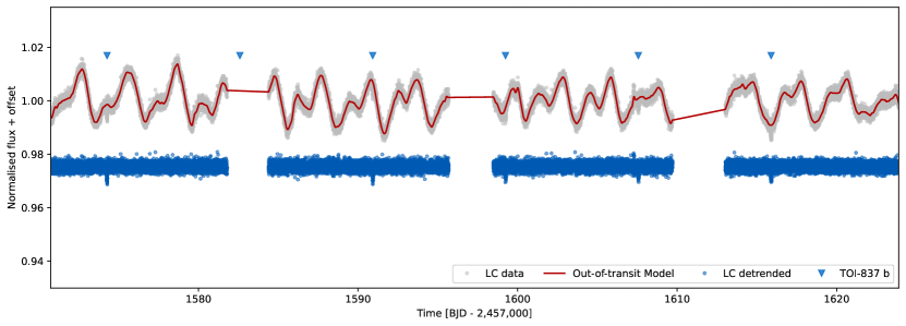
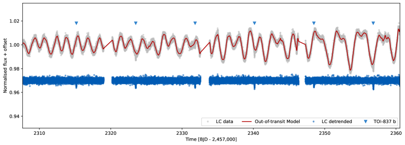
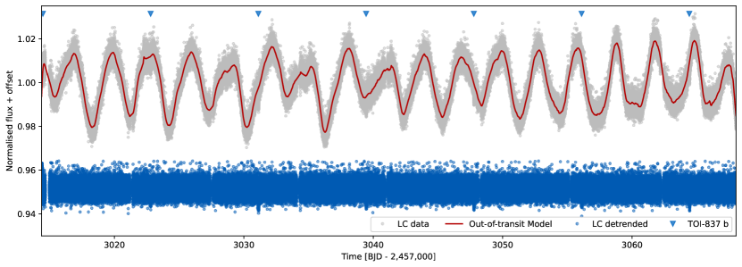
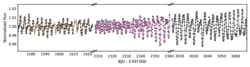
During cycles 3 and 5, TOI-837 was reobserved in Sectors 37 and 38 (from 2021 April 02 to 2021 May 26, with 2 min cadence) and Sectors 63 and 64 (2023 Mar 10 to 2023 May 04, with 20 s cadence), respectively. We downloaded the Presearch Data Conditioning Simple Aperture Photometry (PDCSAP; Smith et al., 2012; Stumpe et al., 2012, 2014) light curves for TOI-837 from the Mikulski Archive for Space Telescopes (MAST). Figure 1 shows the TOI-837’s light curves for all the three TESS cycles. TOI-837 will be re-observed by TESS in Sector 90 during the first semester of 2025.
To perform the transit analysis we flattened the TESS light curves (see Sect. 3.2). The TESS light curves for TOI-837 exhibit variations outside of transits, possibly due to stellar or instrumental variability. The TESS light curves were detrended using the open-source code citlalicue \faGithub (Barragán et al., 2022a). In essence, citlalicue employs GPs, as implemented in george (Ambikasaran et al., 2015), to model light curve fluctuations outside of transits. We provided citlalicue with normalised light curves and the ephemeris for the transit signal. To focus on removing low-frequency signals, we used data binned at 3-hour intervals and masked all transits when fitting the GP with a Quasi-Periodic kernel (as in Ambikasaran et al., 2015). We applied an iterative maximum Likelihood optimisation coupled with a -sigma clipping technique to identify the best model for light curve variations outside of transits. Subsequently, we divided the entire light curves based on this model, resulting in a flattened curve showing only transit signals. It is worth noting that each TESS cycle was detrended individually. The detrended light curves for all TESS cycles are presented in Figure 1.
2.2 Ground-based photometric data
B20 performed multi-band ground based follow-up of TOI-837. For full details on the acquisition and reduction we refer the reader to that paper. Four transit events were monitored using the 0.36-meter telescope at El Sauce Observatory, situated in Chile’s Río Hurtado Valley. The data collection occurred during specific nights: the Cousins-R band was used on April 1 and 26 of 2020, the Cousins-I band on May 21, 2020, and the Johnson-B band on June 14, 2020. TOI-837 was also observed by the Antarctic Search for Transiting Exoplanets (ASTEP) telescope at the Concordia base on the Antarctic Plateau, on the dates of May 12, May 29, June 14, and June 23 of 2020. We downloaded all these public data to include them in our analyses.
2.3 HARPS spectroscopic observations
We acquired 75 high-resolution (R 115 000, wavelength range of 380 to 690 nm) spectra of TOI-837 with the High Accuracy Radial velocity Planet Searcher (HARPS; Mayor et al., 2003) spectrograph. The instrument is mounted at the 3.6 m ESO telescope at La Silla Observatory, Chile.
The observations were carried out between October 03 2022 and January 16 2023, as part of the observing program 0110.C-4341(A) (PI: Yu). The typical exposure time per observation was 1800 s, except for the observations before October 25 where the exposure time was set to 900 s. This produced spectra with a typical signal-to-noise (S/N) of 50 (30 for the 900s exposures) at 550 nm.
We post-processed the 1-D spectra produced by the official data reduction software (DRS). All the spectra were first continuum normalised by RASSINE \faGithub (Cretignier et al., 2020b), an upper envelope method fitting the spectra continua . The normalised spectra time series was then post-processed by YARARA (Cretignier et al., 2021). Given the limited S/N of the observations, we restricted the cleaning by YARARA to cosmic rays and tellurics which are the only notable features at such a level of flux precision. From this step onwards, four observations were rejected by YARARA based on an anomalous number of detected outliers. Those spectra were all very low S/N observations (). Once spectra were corrected of systematics, the normalised flux spectra were scaled back to absolute flux units spectra by using a reference continuum111Sometimes referred as a “reference colour”. where the bolometric flux of the spectra was preserved during the scaling:
This step is equivalent in practice to the colour correction usually performed on the order-by-order CCFs to remove any dependency with airmass or weather condition (Lovis, 2007; Cretignier, 2022). We extracted the RVs by a Gaussian fit on CCFs obtained using the G2 mask of the HARPS DRS since for fast-rotating stars, the empirical line list (see e.g., Cretignier et al., 2020a) obtained from the observations could be imperfect due to a large number of blends.
Our HARPS RV measurements have a typical error of 10 and a RMS of 100 . The full width at half maximum (FWHM) of the CCF shows a consequent broadening with a value around FWHM in agreement with the fast rotation rate of the star (see Sect. 3.1). Table 2 lists the extracted HARPS RVs, FWHM, Bisector span (BIS), calcium lines S-index (), and Hydrogen-alpha () time series.
| Time | RV | FWHM | BIS | S/N (550 nm) | |||||||
|---|---|---|---|---|---|---|---|---|---|---|---|
| - 2 470 000 | |||||||||||
| 2855.882062 | 0.0634 | 0.0160 | 24.0112 | 0.0521 | -0.0708 | 0.0216 | 0.0386 | 0.0242 | 0.3979 | 0.0039 | 27 |
| 2859.873603 | -0.0075 | 0.0155 | 23.8725 | 0.0505 | -0.0957 | 0.0210 | 0.0811 | 0.0238 | 0.3918 | 0.0035 | 29 |
| 2860.880897 | 0.0386 | 0.0206 | 23.7631 | 0.0671 | -0.4361 | 0.0278 | 0.0255 | 0.0347 | 0.3972 | 0.0048 | 23 |
| 2861.882173 | 0.1588 | 0.0172 | 24.0269 | 0.0560 | -0.3255 | 0.0232 | 0.0683 | 0.0302 | 0.3954 | 0.0041 | 26 |
| 2863.879982 | 0.0442 | 0.0152 | 23.9185 | 0.0493 | -0.3695 | 0.0204 | -0.0254 | 0.0214 | 0.3899 | 0.0031 | 32 |
2.3.1 Periodograms
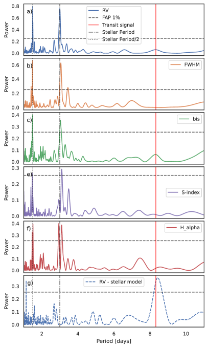
As a first check to test the information contained in our HARPS spectroscopic time series, we ran a General Lomb-Scargle (GLS; Zechmeister & Kürster, 2009) periodogram on them. Figure 2 shows the periodogram of all the time series. We can see that all of the spectroscopic time series peak around and d, which correspond to the rotational period of the star and its first harmonic. The peaks at the stellar rotation period and its first harmonic suggest the presence of active regions on the stellar surface (e.g., Aigrain et al., 2012). No substantial peak corresponding to the orbital period of TOI-837 b is evident in the raw RVs.
3 Data analysis
3.1 Stellar parameters
3.1.1 Atmospheric parameters
We used the HARPS spectra to derive the atmospheric parameters of TOI-837. As this star is a fast rotator, we analysed the spectra using spectral synthesis. Two different methods were employed, FASMA-synthesis222https://github.com/MariaTsantaki/FASMA-synthesis and PAWS333https://github.com/alixviolet/PAWS, as well as two different sets of spectra, the DRS spectra and the YARARA-processed spectra (see Sect. 2.3). Each set of spectra was shifted in the lab frame and co-added and the analyses were performed on this co-added spectrum.
FASMA-synthesis made use of the MARCS atmospheric models (Gustafsson et al., 2008) and the radiative transfer code MOOG444https://www.as.utexas.edu/~chris/moog.html. Micro- and macroturbulent velocities were calculated through the calibration relations mentioned in Tsantaki et al. (2013) and Doyle et al. (2014), respectively. More details on this method can be found in Tsantaki et al. (2020).
PAWS uses the functionalities from iSPEC (Blanco-Cuaresma, 2019) and is described in more detail in Freckelton et al. (2024). We used the Kurucz atmospheric models in our analysis (Kurucz, 1993) and skipped the initial step of the equivalent width analysis as this is less reliable for fast rotators where the spectral lines are broadened.
These four analyses provided values for the effective temperature, the surface gravity, the metallicity, and the projected rotational velocity. All values are in agreement with their 1-sigma errors. For our adopted parameters, listed in Table 1, we choose to take a weighted average of all the results. The high value of the projected rotational velocity (16.8 km/s) confirms the fast-rotating nature of TOI-837. All other parameters are close to Solar values.
3.1.2 Mass, radius, and age
To calculate the fundamental stellar parameters, we made use of the isochrones (Morton, 2015) package. Our stellar models came from the MESA Isochrones and Stellar Tracks (MIST - Dotter, 2016) and we used the nested sampler MultiNest (Feroz et al., 2019) for our likelihood analysis. As input data, we used the photometric magnitudes B, V, J, H, Ks, W1, W2, W3, the Gaia DR3 parallax, and the spectroscopically derived effective temperature and metallicity. In a similar way as described in Mortier et al. (2020), we ran the code four times, each time changing the spectroscopic input to the individually obtained results and keeping the other data the same. Narrow bounds were set on the stellar age, between 30 and 46 Myr, following B20, which helps constrain the stellar mass given strong correlations between mass and age for young stars.
After checking that all parameters from the individual runs agreed within errors, the final parameters and errors, listed in Table 1, were obtained from the median and 16th/84th percentile of the combined posterior distributions of the four runs. The mass and radius values are, unsurprisingly, close to Solar values. From these, we can recalculate a much more precise value of the surface gravity. It is lower than, but consistent with, the spectroscopically derived surface gravity. Using the stellar radius and the projected rotational velocity, we can furthermore also place an upper limit on the stellar rotation period. We find that the rotation period has a maximum value of d. This is fully compatible with the values obtained with TESS and spectroscopic time series (see Sect. 3.3).
3.2 Transit analysis
For all the subsequent planet analyses we used the code pyaneti \faGithub (Barragán et al., 2019a, 2022a). In all our runs we sample the parameter space with 250 walkers using the Markov chain Monte Carlo (MCMC) ensemble sampler algorithm implemented in pyaneti \faGithub (Barragán et al., 2019a; Foreman-Mackey et al., 2013). The posterior distributions are created with the last 5000 iterations of converged chains. We thinned our chains by a factor of 10 giving a distribution of 125 000 points for each sampled parameter.
To speed up the transit modelling, we only model data chunks spanning a maximum of three hours on either side of each transit mid-time. TESS and ground-base photometry were acquired with short cadence ( min). Therefore we can assume that this data can be described by instantaneous evaluations of the transit models and we do not need model re-sampling (see e.g., Gandolfi et al., 2018). In total we have six different photometric data sets named: TESS 2 min data (cycles 1 and 3), TESS 25s data (cycle 5), ASTEP, and El Sauce R, I, and B bands.
To model the transits of TOI-837 b, we need to set priors for the following set of parameters: time of mid-transit, ; orbital period, ; orbital eccentricity, and angle of periastron, using the polar parametrisation and ; scaled planetary radius ; the stellar density, ; and the the limb darkening parameters and for each band (following Mandel & Agol, 2002; Kipping, 2013, models and parametrisations). We assume a black object transit and we sample for a single for all bands (B20 showed that there is no variation of in different bands). The scaled semi-major axis, , is recovered from and Kepler’s third law (see e.g., Winn, 2010). The model also includes photometric jitter term per data set to penalise the likelihood. We start by assuming that the orbit is circular, so we fix . For the rest of parameters we set wide informative uniform priors as listed in Table 3.
To start our transit analysis, it is worth mentioning that TOI-837 b’s transit looks V-shaped, indicating that the transit could be grazing (where the grazing condition is given when ). B20 reported and , suggesting that the transit is either grazing or nearly grazing. We note that B20 performed this analysis using the available data at the time: TESS cycle 1 and the ground-based data. We performed an analysis using exactly this data set, and we obtained fully consistent results of and . The small differences with B20 can be explained by the different ways to deal with the detrending and/or different parametrisations.
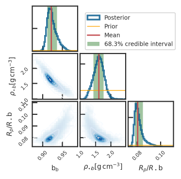
We then repeated the analysis including the new data of the TESS cycles 3 and 5. We obtained more precise values of and . These values are still consistent with a grazing transit. Figure 3 shows a correlation plot between , , and . We can see that the grazing condition covers only the low probability tail of the posterior distribution. Therefore, we are able to put strong constraints on the inferred planetary radius.
It is also worth mentioning that the stellar density recovered from the transit analysis, , is fully consistent with the stellar parameters derived in Section 3.1. This suggests that the planetary orbit is nearly circular. To test this further, we performed another transit analysis where we used a Gaussian prior on the stellar density using the value in Table 1. We also sample for the orbit eccentricity using the polar parametrisation and . We inferred and that relates to an eccentricity of . These results are consistent with a nearly circular orbit for TOI-837 b. It is also worth mentioning that the model with a circular orbit is strongly preferred over the model with eccentricity with a difference of Akaike Information Criterion ( AIC) of 52. We then conclude that the photometric data strongly prefers a model assuming a circular orbit. Figure 4 shows TOI-837 b’s transits for the different data sets with the respective inferred models.

| Parameter | Prior(a) | Final value(b) |
| TOI-837 b’s parameters | ||
| Orbital period (days) | ||
| Transit epoch (BJD2 470 000) | ||
| Scaled planet radius | ||
| Impact parameter, | ||
| 0 | ||
| 0 | ||
| Doppler semi-amplitude, () | ||
| GP hyperparameters | ||
| GP Period (days) | ||
| (days) | ||
| () | ||
| Other parameters | ||
| Stellar density () | ||
| TESS Parameterised limb-darkening coefficient | ||
| TESS Parameterised limb-darkening coefficient | ||
| El Sauce-R Parameterised limb-darkening coefficient | ||
| El Sauce-R Parameterised limb-darkening coefficient | ||
| El Sauce-I Parameterised limb-darkening coefficient | ||
| El Sauce-I Parameterised limb-darkening coefficient | ||
| El Sauce-B Parameterised limb-darkening coefficient | ||
| El Sauce-B Parameterised limb-darkening coefficient | ||
| ASTEP Parameterised limb-darkening coefficient | ||
| ASTEP Parameterised limb-darkening coefficient | ||
| Jitter term (ppm) | ||
| Jitter term (ppm) | ||
| Jitter term (ppm) | ||
| Jitter term (ppm) | ||
| Jitter term (ppm) | ||
| Jitter term (ppm) | ||
| HARPS offset () | ||
| HARPS Jitter, () | ||
| TOI-837 b’s derived parameters | ||
| Planet radius, () | ||
| Planet mass, () | ||
| Planet density, (g cm-3) | ||
| Scaled semi-major axis | ||
| semi-major axis (AU) | ||
| Orbital inclination (deg) | ||
| Equilibrium temperature(c) () | ||
| Transit duration (h) | ||
| Planet surface gravity ()(d) | ||
| Planet surface gravity ()(e) | ||
| Insolation () | ||
| a refers to a fixed value , to an uniform prior between and , to a Gaussian prior with mean and standard deviation , | ||
| and to the modified Jeffrey’s prior as defined by Gregory (2005, eq. 16). | ||
| b Inferred parameters and errors are defined as the median and 68.3% credible interval of the posterior distribution. | ||
| c Assuming an albedo of zero. | ||
| d Derived using . | ||
| e Derived using sampled parameters following Southworth et al. (2007). | ||
3.3 Characterising the stellar signal
Because of its youth, TOI-837 has strong stellar signals in its light curve and RVs time series. We performed several analyses of the light curves and spectroscopic time series to analyse the time scales over which the stellar signal evolves.
3.3.1 Stellar signal in the TESS light curves
We first performed a onedimensional GP regression of the TESS light curves to study the behaviour of the stellar signal at the different TESS cycles. Since we are interested in modelling the long-term evolution of the light curve, we binned the data into 3 hour chunks and masked the transits out of the light curve.
We model the covariance between two data points at times and for each time-series as
| (1) |
where is an amplitude term, and is the Quasi-Periodic (QP) kernel given by
| (2) |
whose hyperparameters are: , the GP characteristic period; , the inverse of the harmonic complexity; and , the long-term evolution timescale.
We sample 5 parameters in each run: four GP hyperparameters (, , , ), and a jitter term included in the Gaussian Likelihood. We set wide uniform priors for all the parameters: for we set a uniform prior between 0.1 and 100 d, for between 0.1 and 5, and for between 2.5 and 3.5 d. We sample the parameter space using the built-in MCMC sampler in pyaneti \faGithub using the same criteria as in Sect. 3.2.
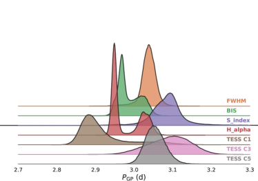
Table 4 shows the inferred , , and hyperparameters for all the light curves. Figure 5 shows the inferred posterior distributions for the , , and parameters for all the modelled time series. Figure 6 shows the TESS light curves with the inferred GP model. The first thing we observe is that the recovered is consistent within the maximum rotational period derived in Section 3.1. However, the rotational period obtained from TESS Cycle 1 is consistent with Cycles 3 and 5 just at 3 sigma. This could be evidence of differential rotation. This can also be caused by the relatively short evolution time-scale recovered that is smaller than the inferred period (see e.g., Rajpaul et al., 2015). We note that all the hyperparameters seem consistent between the different light curves. This is unusual for young stars given that each TESS cycle happens two years after another and the evolution of stellar activity can manifest as different signals that can be explained by different GP hyperparameters (e.g., Barragán et al., 2021).

| Time-series | [d] | [d] | |
|---|---|---|---|
| TESS cycle 1 | |||
| TESS cycle 3 | |||
| TESS cycle 5 | |||
| FWHM | |||
| BIS Span | |||
3.3.2 Stellar signal in the activity indicators
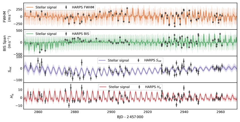
We performed an individual analysis of each activity indicator as the one presented in Barragán et al. (2023). We analyse the FWHM, BIS, , and spectroscopic time series. Note that, in comparison with Section 3.3.1, we are now facing a more difficult signal characterisation given that the spectroscopic time series are not as well sampled as the TESS light curves.
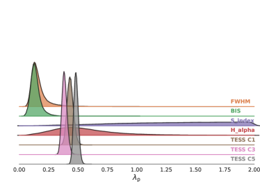
In Section 2.3.1 we show how all the spectroscopic time-series periodograms show significant peaks around 3 and 1.5 d, which are related to the stellar rotational period and its first harmonic, respectively. To better characterise the periodic signals and analyse further signal complexity, we performed a GP regression on each time series using the 1D modelling setup as the one presented in Sect. 3.3.1. We sample for 6 parameters in each run, the kernel hyperparameters (, , , ), an offset, and a jitter term. The priors used were uniform with the ranges: for between 0.1 and 100 d (that corresponds to the HARPS observing window), between 0.1 and 2, and for between 2.5 and 3.5 d.
Table 4 and Figure 5 summarise the inferred GP hyperparameters. Figure 6 shows the spectroscopic time-series data together with the inferred GP model. The first thing we note is that all activity indicators can recover a period that is consistent with the stellar rotation period. This is consistent with the results found in the periodogram analysis (even the double peak observed in the periodogram is presented in the recovered posterior, see Sect. 2.3.1). We were expecting a better agreement between the hyperparameters recovered from the spectroscopic time series (see Barragán et al., 2023). From Figure 6 we can see by eye that the recovered process in each time series looks significantly different. The processes recovered to explain FWHM and BIS Span present variations that are shorter than the time sampling of the HARPS data, this behaviour can be a result of overfitting (see Blunt et al., 2023). We can also see that the recovered signals for and are consistent with a low harmonic complexity process. Barragán et al. (2023) noted that this behaviour can be caused by relatively high white noise that does not allow to characterise the complexity of the underlying signal.
These results suggest that the stellar signal in the activity indicators time series cannot be characterised assuming it behaves as a GP. The rotation period of the star of 3 days is short compared with our sampling strategy of taking one point per night. Three points may not be enough to sample the complexity of the stellar signal, especially if this signal is expected to vary significantly in short time scales, as suggested by the TESS photometry. Therefore, our GP regression may not be able to characterise in full the stellar signal. Furthermore, the rotation period of the star is close to the integer of 3 d. This has as a consequence that observations do not sample properly the phase of the stellar rotation given that observations happen at similar times during the whole observing run. This is worsened in the case in which the stellar signal evolves drastically between each period.
We conclude that for our spectroscopic time series, we can constrain the rotation period of the star. However, any further complexity pattern that may exist cannot be characterised by our dataset. Because of this lack of information on the activity indicators, we conclude that this data set is not a good target to perform multi-dimensional GP regression.
3.4 RV analysis
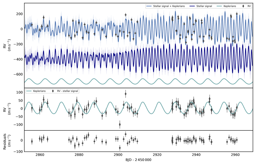
We also performed onedimensional GP modelling to the RVs time series. We first ran a model identical to the GP analyses in Sect. 3.3.2. This means that we sample for the QP kernel hyperparameters (, , , ), and a jitter term. As a mean function, we included just an offset (with no Keplerian model yet). For the GP hyperparameters, we use the same priors as the ones described in Sect. 3.3.2. We recover the hyperparameters d, d, and . We can see that besides the period, the hyperparameters do not compare with any of the hyperparameters obtained from the other spectroscopic time series (see Table 4).
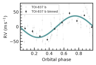
We then repeated the analysis but this time we added a mean function that includes an offset and a Keplerian model to account for the Doppler effect of TOI-837 b. For the planet model we assume a circular orbit, we set Gaussian priors for the planet ephemeris based on the analysis in Sect. 3.2. For the Doppler semi-amplitude we set a uniform prior between 0 and 100 . We inferred hyperparameters fully consistent with the no-planet model; d, d, and . We also recovered a Doppler semi-amplitude of . If this signal is caused by TOI-837 b, that would correspond to a planetary mass of .
When comparing both models, the one with the planetary signal is strongly favoured with a . It is also worth mentioning that the recovered jitter term for the model with the planet signal is , while with no-planet is . This is also evidence that the model that better adjusts the data is the one where the planetary signal is included.
3.5 Final joint model
Based on the analyses presented in this section, our final model for the photometric data of TOI-837 is the transit model described in Section 3.2, together with the RV model described in Sect. 3.4. For completeness, we ran a final joint model of photometry and RVs to characterise TOI-837 b. The whole set of sampled parameters and priors are shown in Table 3.
We also explored a solution where we allowed for an eccentricity. We inferred an orbital eccentricity of . However, the model including a circular orbit is slightly preferred with . This suggests that the orbit of TOI-837 b is (close to) circular and the data we have is not enough to measure any small deviation from it.
4 Discussion
4.1 RV detection tests
We know a priori that TOI-837 b exists and its nature is consistent with being planetary (B20). Therefore, we expect that there is a Doppler signal larger than zero that is consistent with the ephemeris of the transiting signal. If we assumed that TOI-837 b has the same properties as similar planets with its radius, we estimated a mass of that would generate a Doppler signal of (Chen & Kipping, 2017). Due to its youth ( Myr), we would expect a rather lower density object with a significantly smaller mass (e.g., Baraffe et al., 2008; Fortney et al., 2007). Our detected Doppler semi-amplitude is which translates to a mass of for TOI-837 b. This mass together with the inferred radius of results in a planetary density of . This unexpected high density on young giant planets has been found previously (Suárez Mascareño et al., 2021), but the RV detection of such planets are challenged by the community (e.g., Blunt et al., 2023). In this section, we test the reliability of our detection of the induced Doppler signal on TOI-837.
4.1.1 Planet signal in periodograms
As shown in Section 2.3.1 and Figure 2 there is no evidence of the planetary signal in RV GLS periodogram of TOI-837. This is expected given that any planetary signal would be dwarfed by the relatively high stellar activity signal.
We then took the residuals that we obtained from the no-planet onedimensional GP analysis presented in Sect. 3.4 and we applied a GLS periodogram that is shown in the bottom panel of Figure 2. We can see that the peaks that correspond to the stellar signal disappeared from the periodogram, indicating that the GP model was able to remove the intrinsic stellar signal in the RV time series. Furthermore, a significant peak appeared close to the orbital period of the planet. This result is unexpected. GPs have been proven to engulf planetary signals, especially when the latter ones are not included in the model (e.g., Ahrer et al., 2021; Rajpaul et al., 2021). We speculate that if a relatively strong coherent signals is present in our data set, it may survive a GP regression if it evolves with significantly different time scales than the stellar signal. This assumption is consistent with the recovered Doppler signal of TOI-837 b.
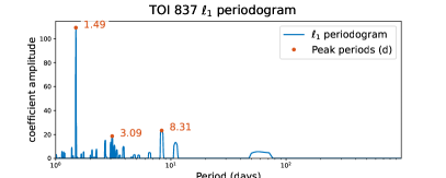
To explore further the existence of the planetary signal in the periodogram, we ran a periodogram (Hara et al., 2017) on the raw RV time series. Briefly, the 1-periodogram is a variation of the Lomb-Scargle periodogram methodology that has reduced sensitivity towards outliers and non-Gaussian noise. Figure 9 shows the 1-periodogram applied to the raw RV time-series of TOI-837. The three most significant peak happens at 1.5, 8.31 and 3.09 d that correspond to the first harmonic of the rotation period of the star, the planet orbit, and the rotation period of the star, respectively. This suggests that there is a strong deep-seated signal that coincides with the orbital period of TOI-837 b. This result supports our previous speculation that there is evidence of strong coherent signal in the RVs that is consistent with our TOI-837 b’s recovered Doppler signal.
4.1.2 Cross-validation
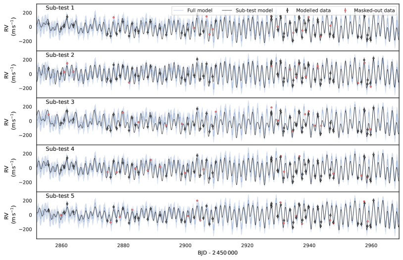
The next test we perform is cross-validation to check for overfitting as suggested by Blunt et al. (2023). To do so, we employ a data partitioning strategy similar to the principles of k-fold cross-validation (see e.g., Fazekas & Kovacs, 2024) to systematically divide our dataset into distinct subsets. Specifically, we first randomised the dataset to ensure that each partition is representative of the overall data distribution. Subsequently, we segmented the dataset into five partitions. In each iteration, we use four out of these five partitions (constituting approximately 80% of the data) for the modelling, while the remaining partition (approximately 20% of the data) is masked out. This approach guarantees that each unique subset serves as the test set exactly once, eliminating any potential overlap between masked-out data across all iterations. Figure 10 shows the five different sub-samples created with this approach.
We then perform a RV analysis (accounting for the planet signal) as the one presented in Sect. 3.4 for each sub-sample, we call each one of these runs as sub-test , where runs between 1 and 5. Figure 10 shows the data and recovered model for all cases. The recovered Doppler semi-amplitude for each case is fully consistent with the value reported in Sect. 3.4, but with slightly larger error bars, as expected due to the smaller number of data modelled. We can see that, by eye, the masked-out points fall well within the limits of the inferred models in each case, suggesting that the predictive model in each case can explain the masked-out observations (see also discussion in Luque et al., 2023). We can also see that the predictive model for each sub-set (black lines) falls well within the confidence intervals of the predictive distribution of the model of the full data set (blue lines and shaded region). These results suggest that our model does not suffer overfitting.
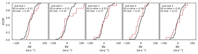
To assess further the reliability of our cross-validation, we perform a Two-sample Kolmogorov-Smirnov (KS; Kolmogorov, 1933; Smirnov, 1948) test. Briefly, the KS test is a non-parametric statistical test that is utilised to validate the hypothesis that two subsets of data originate from the same continuous distribution. This test compares the empirical cumulative distribution functions (ECDFs) of two samples without making any assumptions about the underlying distribution of data. The maximum absolute difference between the ECDFs of the two samples, known as the KS statistic, serves as the basis for evaluating the null hypothesis that the two samples are drawn from the same distribution. A low KS statistic, accompanied by a high p-value, indicates a failure to reject the null hypothesis, suggesting that the differences between the two samples could be attributed to random variation, and hence, they can be considered as coming from the same distribution.
We apply the KS test to each one of our sub-tests in which we compare the residuals of the modelled data with the residuals of the masked-out data (i.e., masked-out points minus predictive distribution at their respective times). If the KS test proves that both samples are explained from the same distribution, then we can conclude that the predictive model explains well the masked-out data. This implies that the inferred model has the ability to explain unseen data, thus, it does not overfit. Figure 10 shows the ECDF for the modelled and masked-out data for each one of the sub-tests. The p-values of the five sub-tests are significantly larger than 0.05, therefore, we can conclude that both samples are consistent with being described by the same underlying distribution. These results give us confidence that our RV model for TOI-837 does not suffer from overfitting.
4.1.3 Injection tests
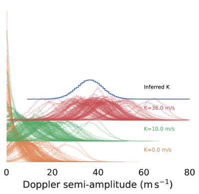
Previous research indicates that complex models can generate false planet-like RV time series, particularly in stars with high activity levels (e.g., Rajpaul et al., 2016). To check if this is our case, we performed injection tests similar to the ones presented in Barragán et al. (2019b); Zicher et al. (2022). We used citlalatonac (Barragán et al., 2022a) to simulate synthetic RV time series at the same time-stamps as our HARPS data. We first took the predictive distribution for the stellar signal that we obtained for TOI-837 in Sect. 3.4. We then added correlated noise using a squared exponential kernel with a length scale of one day, and the same amplitude as the jitter term obtained from the real data to simulate the red noise in our data. To finish, we also added white noise for each synthetic observation according to the nominal measurement uncertainty of each HARPS datum. We created 100 different realisations of stellar-like signals. For each stellar-like signal, we created 3 different types of RV time series injecting signals with Doppler semi-amplitudes of 0 (assuming there is no planet), 10 (expected signal of this planet if it were inflated), and 36 (the recovered signal). This leads to a total of 300 synthetic RV time series with similar noise properties and the same time sampling as the real data.
We model each synthetic dataset using a one-planet model and onedimensional GP configuration as described in Sect. 3.4. We plot the recovered posterior distribution of the Doppler semi-amplitude of the planet for all the runs in Figure 11.
We first check the percentage of the simulations in which we can claim a detection.
For this purpose, we consider that a detection has occurred if the median of the posterior is larger than 3-, where is half the interval between the and percentiles.
We found that we can claim a detection of 4%, 28%, and 100% for the synthetic time series with injected signals of 0, 10, and 36 , respectively.
We then revise which percentage of these detections is consistent with our detection in the real data set. We check what fraction of the time the recovered semi-amplitude in the synthetic time series is within 1- of the recovered posterior distribution from the real data set.
We found that this condition is filled in 0%, 2%, and 55% of the cases for the 0, 10, and 36 time series, respectively.
These results suggest that if the real Doppler signal presented in our RV time-series was 10 we would detect the 36 signal with a probability of 2%.
The 55% recovered in the 36 case is consistent with the expected value taking into account Poisson counting errors.
For the remainder of the paper, we will assume that our mass and radius measurements of TOI-837 b are reliable. Below we describe the physical implications of this for the planet’s properties.
4.2 TOI-837b’s properties
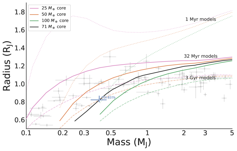
With a mass of and radius of , TOI-837 b’s position in the mass-radius diagram is highlighted in Fig. 12. Figure 12 also shows a mass-radius diagram for giant exoplanets ( and ) detected with a precision better than 30% in radius and mass. Considering that the evolution of planets is influenced by their distance from their host star, we only present planets that orbit within a semi-major axis range of 0.08 to 1 AU. This selection is informed by the semi-major axis of TOI-837 b, AU, and is supported by models that forecast a comparable evolution for planets situated within this range of semi-major axes (see Fortney et al., 2007). We also over plot the Fortney et al. (2007)’s models with similar parameters to those of TOI-837 b. This corresponds to models for planets around a solar-like star, with an age of 32 Myr, at a distance of 0.1 AU with cores of 25 (pink), 50 (orange) and 100 (green) . We performed a radial basis function interpolation on the aforementioned Fortney et al. (2007)’s models to find the core mass that best describes the mass and radius of TOI-837 b. We found that the position and age of TOI-837 b would be consistent with a young planet with a core mass of , assuming a 50-50% ice-silicate core (black line in Fig. 12). This core mass corresponds to of TOI-837 b total mass of .
From figure 12, we can see that if well there are planets that fall close to TOI-837 b in the mass vs radius diagram, they all are older than 1 Gyr and they should be compared with older planet’s models. This can be done from figure 12 where we also show the Fortney et al. (2007)’s models for planets aged 3 Gyr with orbital semi-major axis of 0.1 AU. The first thing we see is that the older counterparts of TOI-837 b are consistent with planets with cores . If TOI-837 b itself was older, we would estimate a significantly smaller core of , our estimation of is a pure consequence of the expected inflated state, hence larger radius, given its youth. In this line of thought, TOI-837 b stands out as the only planet with a semi-major axis of AU consistent with a core.
We then relaxed our assumptions and proceed to compare TOI-837 b with planets with similar mass and radius, but without constrain on their semi-major axes. We found that K2-60 b (Eigmüller et al., 2017), HD 149026 b (Sato et al., 2005), and TOI-1194 b (Wang et al., 2023) are denser than TOI-837 b and are consistent with core masses between despite being significantly older ( Gyr). This suggests that planets with relatively similar masses to TOI-837 b and large cores can exist. The question now is what physical mechanisms can create such massive cores. Johnson & Li (2012) theorised that a star’s high metallicity might reflect a primordial circumstellar disc with elevated dust content that could potentially enhance core formation. Both, HD 149026 b and TOI-1194 b have super-solar atmospheric metallicities that are consistent with this model. In fact, Bean et al. (2023) observed a significant atmospheric metal enrichment on the atmosphere of HD 149026 b that is explained by a bulk heavy element abundance of 66% of the planetary mass. However, the solar metallicity of TOI-837 and K2-60 does not support this hypothesis, suggesting that other factors may also play a critical role in the formation of massive cores. Boley et al. (2016) proposed a theory where massive cores, with masses exceeding , could result from the merging of tightly packed orbiting inner planets that formed during the initial phases of the circumstellar disc’s evolution.
Another possibility is that TOI-837 b has a less massive core, but the models are biased towards larger radii for young planets.
Core-accretion models of planetary evolution predict planets of
Myr to be at the early stages of their contraction phase, showing very large radii and low densities (Baraffe et al., 2008; Fortney et al., 2007, see also 1 Myr models in Fig. 12).
However, Fortney et al. (2007)’s models do not include a formation mechanism and can be arbitrarily large and hot at very young ages (see Marley et al., 2007). This can lead to giant planet’s models with radii several tenths
of a Jupiter radius larger than one computed taking into account formation mechanisms. This would lead as a consequence to estimate more massive cores for a given planet’s mass and radius.
For the remainder of the paper we will assume that TOI-837 b can be described by Fortney et al. (2007)’s models assuming a core of .
4.3 Atmospheric characterisation perspectives
Atmospheric observations could play a crucial role in differentiating among various potential formation mechanisms for TOI-837 b. According to the mass-metallicity relationship empirically established by Thorngren et al. (2016), our mass measurement of TOI-837 b suggests a predicted metal fraction ratio between the planet and its host star of . With TOI-837’s stellar metallicity measured at , this translates into an estimated bulk metallicity fraction for TOI-837 b of . Bean et al. (2023) presents a relationship between atmospheric and bulk metallicity fractions. If we assume that TOI-837 b follows this trend, we could expect its atmospheric metallicity to surpass solar values by a factor of . This significant enhancement in atmospheric metallicity would not only support the substantial core mass inferred from our observations but also provide insight into the planet’s formation conditions and subsequent evolutionary history.
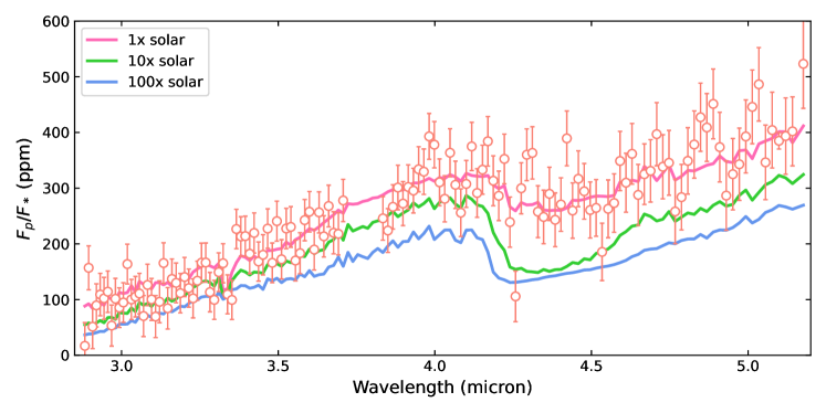
To predict the observability of the atmosphere of TOI-837 b with JWST, we leverage packages picaso555https://natashabatalha.github.io/picaso/ and pandexo666https://natashabatalha.github.io/PandExo/index.html. We forward model the emission spectrum of TOI-837 b using picaso (Batalha et al., 2019), based on the parameters derived in this work. We make use of the integrated 1D climate modelling for the temperature-pressure (TP) profile and chemical abundance solution (Mukherjee et al., 2023), including all opacities available in picaso. The TP profile includes a convective zone only in the deepest atmospheric layers. We then use pandexo to estimate the signal-to-noise of the dayside emission signal of TOI-837 b with JWST/NIRSpec G395H; the predicted observations using three eclipses are shown in Fig. 13, assuming solar metallicity and C/O. At least two eclipse observations are needed to distinguish between a and solar metallicity scenario. Using the chi-square statistic for hypothesis testing, we would expect to distinguish between these cases to a significance of with two eclipse observations (totalling 10.01 hrs), rising to with three eclipses (Fig. 13). Constraining the atmospheric metallicity will help to break the degeneracy with interior composition and the implications for formation.
5 Conclusions
Our investigation into the TOI-837 system and its intriguing companion, TOI-837 b, unveils a young Saturn-sized exoplanet that defies conventional expectations with its unexpected massive core. Our exhaustive analysis of data from TESS ground-based observations, and HARPS spectroscopic enabled us to determine TOI-837 b’s radius at and mass at , translating to a density of . This density together with its age and distance to the star suggest a core mass of approximately 70 , accounting for 60% of the planet’s total mass. Such a substantial core within a relatively young planetary body presents a challenging scenario for current models of planet formation and core accretion, especially due to the relatively low stellar metallicity.
The unique characteristics of TOI-837 b underscore the urgency for advanced atmospheric characterisation. Eclispe observations with JWST could to offer unparalleled insights into the composition of TOI-837 b. A measurement of the planetary atmospheric bulk metal fraction will potentially elucidate the true nature of its significant core. Such future studies are crucial for breaking the current degeneracies in planet composition models and could revolutionise our understanding of planetary formation.
We also leave open the possibility that our RV detection could not be accurate. Despite the tailored campaign with a high cadence of observations, the apparent fast evolution of the strong stellar signal could generate biased measurements of the Doppler semi-amplitude. We showed with several statistical tests that our RV planetary detection is robust, nevertheless, further observations could help us to test this further. For example, tailored near Infrared RV campaigns, where stellar activity is less significant, with instruments such as the Near Infra Red Planet Searcher (NIRPS) could help to assert our detection in the optical.
Acknowledgements
This publication is part of a project that has received funding from the European Research Council (ERC) under the European Union’s Horizon 2020 research and innovation programme (Grant agreement No. 865624). This work made use of numpy (Harris et al., 2020), matplotlib (Hunter, 2007), and pandas (pandas development team, 2020) libraries. This work made use of Astropy:777http://www.astropy.org a community-developed core Python package and an ecosystem of tools and resources for astronomy (Astropy Collaboration et al., 2013, 2018, 2022). This publication made use of data products from the Wide-field Infrared Survey Explorer, which is a joint project of the University of California, Los Angeles, and the Jet Propulsion Laboratory/California Institute of Technology, funded by the National Aeronautics and Space Administration. AVF acknowledges the support of the IOP through the Bell Burnell Graduate Scholarship Fund. OB acknoweledges that the random seed used for the injection simulations was 060196.
Data Availability
The codes used in this manuscript are freely available at https://github.com/oscaribv. The spectroscopic measurements that appear in Table 2 are available as supplementary material in the online version of this manuscript. All TESS data are available via the MAST archive. Ground-based photometry are available on the online version of Bouma et al. (2020).
References
- Ahrer et al. (2021) Ahrer E., et al., 2021, MNRAS, 503, 1248
- Aigrain & Foreman-Mackey (2023) Aigrain S., Foreman-Mackey D., 2023, ARA&A, 61, 329
- Aigrain et al. (2012) Aigrain S., Pont F., Zucker S., 2012, MNRAS, 419, 3147
- Akeson et al. (2013) Akeson R. L., et al., 2013, PASP, 125, 989
- Ambikasaran et al. (2015) Ambikasaran S., Foreman-Mackey D., Greengard L., Hogg D. W., O’Neil M., 2015, IEEE Transactions on Pattern Analysis and Machine Intelligence, 38, 252
- Astropy Collaboration et al. (2013) Astropy Collaboration et al., 2013, A&A, 558, A33
- Astropy Collaboration et al. (2018) Astropy Collaboration et al., 2018, AJ, 156, 123
- Astropy Collaboration et al. (2022) Astropy Collaboration et al., 2022, ApJ, 935, 167
- Baraffe et al. (2008) Baraffe I., Chabrier G., Barman T., 2008, A&A, 482, 315
- Barragán et al. (2018) Barragán O., et al., 2018, A&A, 612, A95
- Barragán et al. (2019a) Barragán O., Gandolfi D., Antoniciello G., 2019a, MNRAS, 482, 1017
- Barragán et al. (2019b) Barragán O., et al., 2019b, MNRAS, 490, 698
- Barragán et al. (2021) Barragán O., Aigrain S., Gillen E., Gutiérrez-Canales F., 2021, Research Notes of the AAS, 5, 51
- Barragán et al. (2022a) Barragán O., Aigrain S., Rajpaul V. M., Zicher N., 2022a, MNRAS, 509, 866
- Barragán et al. (2022b) Barragán O., et al., 2022b, MNRAS, 514, 1606
- Barragán et al. (2023) Barragán O., et al., 2023, MNRAS, 522, 3458
- Batalha et al. (2019) Batalha N. E., Lewis T., Fortney J. J., Batalha N. M., Kempton E., Lewis N. K., Line M. R., 2019, ApJ, 885, L25
- Bean et al. (2023) Bean J. L., et al., 2023, Nature, 618, 43
- Blanco-Cuaresma (2019) Blanco-Cuaresma S., 2019, MNRAS, 486, 2075
- Blunt et al. (2023) Blunt S., et al., 2023, AJ, 166, 62
- Boley et al. (2016) Boley A. C., Granados Contreras A. P., Gladman B., 2016, ApJ, 817, L17
- Bouma et al. (2020) Bouma L. G., et al., 2020, AJ, 160, 239
- Chen & Kipping (2017) Chen J., Kipping D., 2017, ApJ, 834, 17
- Cretignier (2022) Cretignier M., 2022, PhD thesis, University of Geneva, Switzerland
- Cretignier et al. (2020a) Cretignier M., Dumusque X., Allart R., Pepe F., Lovis C., 2020a, A&A, 633, A76
- Cretignier et al. (2020b) Cretignier M., Francfort J., Dumusque X., Allart R., Pepe F., 2020b, A&A, 640, A42
- Cretignier et al. (2021) Cretignier M., Dumusque X., Hara N. C., Pepe F., 2021, A&A, 653, A43
- Cutri et al. (2003) Cutri R. M., et al., 2003, VizieR Online Data Catalog, p. II/246
- David et al. (2018) David T. J., et al., 2018, AJ, 155, 222
- Dotter (2016) Dotter A., 2016, ApJS, 222, 8
- Doyle et al. (2014) Doyle A. P., Davies G. R., Smalley B., Chaplin W. J., Elsworth Y., 2014, MNRAS, 444, 3592
- Eigmüller et al. (2017) Eigmüller P., et al., 2017, AJ, 153, 130
- Fazekas & Kovacs (2024) Fazekas A., Kovacs G., 2024, arXiv e-prints, p. arXiv:2401.13843
- Feroz et al. (2019) Feroz F., Hobson M. P., Cameron E., Pettitt A. N., 2019, The Open Journal of Astrophysics, 2, 10
- Foreman-Mackey et al. (2013) Foreman-Mackey D., Hogg D. W., Lang D., Goodman J., 2013, PASP, 125, 306
- Fortney et al. (2007) Fortney J. J., Marley M. S., Barnes J. W., 2007, ApJ, 659, 1661
- Freckelton et al. (2024) Freckelton A. V., Sebastian D., Mortier A., Triaud A., et a., 2024, submitted to MNRAS
- Gaia Collaboration (2020) Gaia Collaboration 2020, VizieR Online Data Catalog, p. I/350
- Gandolfi et al. (2018) Gandolfi D., et al., 2018, A&A, 619, L10
- Gregory (2005) Gregory P. C., 2005, ApJ, 631, 1198
- Guerrero et al. (2021) Guerrero N. M., et al., 2021, ApJS, 254, 39
- Gustafsson et al. (2008) Gustafsson B., Edvardsson B., Eriksson K., Jørgensen U. G., Nordlund Å., Plez B., 2008, A&A, 486, 951
- Hara et al. (2017) Hara N. C., Boué G., Laskar J., Correia A. C. M., 2017, MNRAS, 464, 1220
- Harris et al. (2020) Harris C. R., et al., 2020, Nature, 585, 357
- Hobson et al. (2021) Hobson M. J., et al., 2021, AJ, 161, 235
- Høg et al. (2000) Høg E., et al., 2000, A&A, 355, L27
- Howell et al. (2014) Howell S. B., et al., 2014, PASP, 126, 398
- Hunter (2007) Hunter J. D., 2007, Computing in Science & Engineering, 9, 90
- Jenkins (2002) Jenkins J. M., 2002, ApJ, 575, 493
- Jenkins et al. (2010) Jenkins J. M., et al., 2010, in Radziwill N. M., Bridger A., eds, Society of Photo-Optical Instrumentation Engineers (SPIE) Conference Series Vol. 7740, Software and Cyberinfrastructure for Astronomy. p. 77400D, doi:10.1117/12.856764
- Jenkins et al. (2016) Jenkins J. M., et al., 2016, in Proc. SPIE. p. 99133E, doi:10.1117/12.2233418
- Jenkins et al. (2020) Jenkins J. M., Tenenbaum P., Seader S., Burke C. J., McCauliff S. D., Smith J. C., Twicken J. D., Chandrasekaran H., 2020, Kepler Data Processing Handbook: Transiting Planet Search, Kepler Science Document KSCI-19081-003
- Johnson & Li (2012) Johnson J. L., Li H., 2012, ApJ, 751, 81
- Kipping (2013) Kipping D. M., 2013, MNRAS, 435, 2152
- Kolmogorov (1933) Kolmogorov A., 1933, G. Ist. Ital. Attuari, 4, 83
- Kurucz (1993) Kurucz R. L., 1993, SYNTHE spectrum synthesis programs and line data. Kurucz CD-ROM
- Li et al. (2019) Li J., Tenenbaum P., Twicken J. D., Burke C. J., Jenkins J. M., Quintana E. V., Rowe J. F., Seader S. E., 2019, PASP, 131, 024506
- Lovis (2007) Lovis C., 2007, PhD thesis, University of Geneva, Switzerland
- Luque et al. (2023) Luque R., et al., 2023, Nature, 623, 932
- Mallorquín et al. (2023) Mallorquín M., et al., 2023, A&A, 680, A76
- Mandel & Agol (2002) Mandel K., Agol E., 2002, ApJ, 580, L171
- Mann et al. (2021) Mann A. W., et al., 2021, arXiv e-prints, p. arXiv:2110.09531
- Mantovan et al. (2023) Mantovan G., et al., 2023, arXiv e-prints, p. arXiv:2310.16888
- Marley et al. (2007) Marley M. S., Fortney J. J., Hubickyj O., Bodenheimer P., Lissauer J. J., 2007, ApJ, 655, 541
- Martioli et al. (2021) Martioli E., Hébrard G., Correia A. C. M., Laskar J., Lecavelier des Etangs A., 2021, A&A, 649, A177
- Mayor et al. (2003) Mayor M., et al., 2003, The Messenger, 114, 20
- Mortier et al. (2020) Mortier A., et al., 2020, MNRAS, 499, 5004
- Morton (2015) Morton T. D., 2015, VESPA: False positive probabilities calculator, Astrophysics Source Code Library (ascl:1503.011)
- Mukherjee et al. (2023) Mukherjee S., Batalha N. E., Fortney J. J., Marley M. S., 2023, ApJ, 942, 71
- Rajpaul et al. (2015) Rajpaul V., Aigrain S., Osborne M. A., Reece S., Roberts S., 2015, MNRAS, 452, 2269
- Rajpaul et al. (2016) Rajpaul V., Aigrain S., Roberts S., 2016, MNRAS, 456, L6
- Rajpaul et al. (2021) Rajpaul V. M., et al., 2021, MNRAS, 507, 1847
- Ricker et al. (2015) Ricker G. R., et al., 2015, Journal of Astronomical Telescopes, Instruments, and Systems, 1, 014003
- Rizzuto et al. (2020) Rizzuto A. C., et al., 2020, AJ, 160, 33
- Sato et al. (2005) Sato B., et al., 2005, ApJ, 633, 465
- Smirnov (1948) Smirnov N., 1948, The Annals of Mathematical Statistics, 19, 279
- Smith et al. (2012) Smith J. C., et al., 2012, PASP, 124, 1000
- Southworth et al. (2007) Southworth J., Wheatley P. J., Sams G., 2007, MNRAS, 379, L11
- Stumpe et al. (2012) Stumpe M. C., et al., 2012, PASP, 124, 985
- Stumpe et al. (2014) Stumpe M. C., Smith J. C., Catanzarite J. H., Van Cleve J. E., Jenkins J. M., Twicken J. D., Girouard F. R., 2014, PASP, 126, 100
- Suárez Mascareño et al. (2021) Suárez Mascareño A., et al., 2021, Nature Astronomy, 6, 232
- Thorngren et al. (2016) Thorngren D. P., Fortney J. J., Murray-Clay R. A., Lopez E. D., 2016, ApJ, 831, 64
- Tsantaki et al. (2013) Tsantaki M., Sousa S. G., Adibekyan V. Z., Santos N. C., Mortier A., Israelian G., 2013, A&A, 555, A150
- Tsantaki et al. (2020) Tsantaki M., Andreasen D., Teixeira G., 2020, Journal of Open Source Software, 5, 2048
- Twicken et al. (2018) Twicken J. D., et al., 2018, PASP, 130, 064502
- Wang et al. (2023) Wang J.-Q., et al., 2023, arXiv e-prints, p. arXiv:2310.12458
- Winn (2010) Winn J. N., 2010, arXiv e-prints, p. arXiv:1001.2010
- Zechmeister & Kürster (2009) Zechmeister M., Kürster M., 2009, A&A, 496, 577
- Zicher et al. (2022) Zicher N., et al., 2022, MNRAS, 512, 3060
- pandas development team (2020) pandas development team T., 2020, pandas-dev/pandas: Pandas, doi:10.5281/zenodo.3509134, https://doi.org/10.5281/zenodo.3509134