Bbbk \savesymbolopenbox \restoresymbolNEWBbbk \restoresymbolNEWopenbox
Interval Abstractions for Robust Counterfactual Explanations
Abstract
Counterfactual Explanations (CEs) have emerged as a major paradigm in explainable AI research, providing recourse recommendations for users affected by the decisions of machine learning models. However, when slight changes occur in the parameters of the underlying model, CEs found by existing methods often become invalid for the updated models. The literature lacks a way to certify deterministic robustness guarantees for CEs under model changes, in that existing methods to improve CEs’ robustness are heuristic, and the robustness performances are evaluated empirically using only a limited number of retrained models. To bridge this gap, we propose a novel interval abstraction technique for parametric machine learning models, which allows us to obtain provable robustness guarantees of CEs under the possibly infinite set of plausible model changes . We formalise our robustness notion as the -robustness for CEs, in both binary and multi-class classification settings. We formulate procedures to verify -robustness based on Mixed Integer Linear Programming, using which we further propose two algorithms to generate CEs that are -robust. In an extensive empirical study, we demonstrate how our approach can be used in practice by discussing two strategies for determining the appropriate hyperparameter in our method, and we quantitatively benchmark the CEs generated by eleven methods, highlighting the effectiveness of our algorithms in finding robust CEs.
1 Introduction
As the field of explainable AI (XAI) has matured, counterfactual explanations (CEs) have risen to prominence as one of the dominant post-hoc methods for explaining the outputs of AI models (see Guidotti (2022); Karimi et al. (2023) for overviews). For a given input to a model, a CE essentially presents a user with a modified input which results in a different output from the model, thus pointing to the reasons for the original output. CEs have been advocated to improve human understanding and trust Miller (2019), as they can help humans build rich mental representations Celar and Byrne (2023). Intially Tolomei et al. (2017); Wachter et al. (2017), CEs were optimised for validity, i.e. correctness in changing the output, and proximity, with respect to some distance measure between the original and modified inputs. Since then, additional metrics have been proposed (see Guidotti (2022) for an overview), such as diversity Mothilal et al. (2020), i.e. how widely CEs differ from one another, and plausibility Dhurandhar et al. (2018), i.e. whether the CEs lie within the data distribution.
A further metric which is receiving increasing attention of late is robustness, i.e. how the validity of a CE is affected by changes in the scenario for which the CE was initially generated. In this paper, we focus on robustness to slight changes in the AI model parameters induced by, for example, retraining Upadhyay et al. (2021); Bui et al. (2022); Black et al. (2022); Dutta et al. (2022); Nguyen et al. (2022); Jiang et al. (2023a, 2024a). This form of robustness is of critical importance in practice. For illustration, consider a mortgage applicant who was rejected by a model and received a CE demonstrating changes they could make to their situation in order to have their application accepted. If retraining occurs while the applicant makes those changes, without robustness, their modified case may still result in a rejected application, leaving the mortgage provider liable due to their conflicting statements. This is especially concerning when CEs are optimised for proximity, as they are likely to be close to the model’s decision boundary and thus at high risk of being invalid if small changes in this boundary occur Upadhyay et al. (2021).
Methods recently introduced to target this problem typically rely on heuristics to induce robustness to model changes, used either directly in a gradient-based optimisation procedure Nguyen et al. (2022); Upadhyay et al. (2021) or post-hoc to refine any candidate CEs found by non-robust CE generation methods Black et al. (2022); Dutta et al. (2022); Hamman et al. (2023). Due to their heuristic nature, these methods lack formal guarantees, which are advocated as being vital towards achieving trustworthy AI Marques-Silva and Ignatiev (2022).
In this work, we present a method which provides deterministic robustness guarantees for CEs, filling the above gap. Specifically, we first define the plausible model changes, , which represents our robustness target. Then, we propose a novel interval abstraction technique, which over-approximates the output node ranges of parametric machine learning models (including neural networks and logistic regressions) when subject to the model changes encoded in . This technique is inspired by the abstraction method in Prabhakar and Afzal (2019), originally proposed for estimating neural networks’ outputs by grouping weight edges into weight intervals. We show that using our interval abstraction, the robustness of CEs under can be formally verified. We formalise such provable robustness as the -robustness of CEs. Unlike most previous robust CE methods which only apply to binary classification, our focus on computing output node ranges allows our method to also work on multi-class classification. Mixed Integer Linear Programming (MILP) is used to practically test -robustness. Using this, we further propose an iterative algorithm operating on existing CEs methods, and a sound and complete Robust Nearest-neighbour Counterfactual Explanations (RNCE) algorithm to generate provably robust CEs. Finally, in an extensive empirical study, we show how our approach can also adapt to capture robustness against unbounded model changes. We demonstrate the effectiveness of our CE generation algorithms in the benchmarking study against seven existing methods. Notably, one configuration of our iterative algorithm finds -robust CEs with the lowest costs among all the robust baselines, and our new RNCE algorithm achieves perfectly robust results while finding CEs close to the data manifold.
The paper is structured as follows. In Section 2 we cover the related work, and in Section 3 we introduce the context of computing CEs with formal notations. Sections 4, 5, and 6 introduce the formalisations for -robustness and the MILP encodings for testing it. Then, the two CEs generation algorithms are presented in Section 7, which are extensively evaluated through experiments in Section 8. We conclude in Section 9 with future research directions. The core contributions of our work are summarised as follows:
-
•
We propose a novel interval abstraction method to test -robustness, deterministically verifying whether a CE is robust against plausible model changes.
-
•
Our method explicitly characterises provable robustness guarantees for CEs in multi-class classification, and, to the best of our knowledge, is the first to do so.
-
•
We introduce an iterative algorithm and the RNCE algorithm to generate provably robust CEs, which are demonstrated to have superior performances against seven baselines.
-
•
We present a principled workflow demonstrating the usefulness of -robustness for evaluating and generating robust CEs in practice.
This paper builds upon our previous work Jiang et al. (2023a) with significant extensions. Specifically, Section 4 extends the corresponding section in Jiang et al. (2023a) to account for different parametric machine learning models in addition to feed-forward neural networks. We present in-depth discussions and relaxations for the soundness of (Definition 9), and formalisations for multi-class classifications are included with an empirical study (Sections 5, 8.5). Section 6 formalises testing procedures for -robustness in terms of MILP programs, which were only briefly mentioned in Appendix B of our previous work. Section 7 significantly extends the algorithm proposed in Jiang et al. (2023a), which could fail to find provably robust CEs. We show that our new algorithm, RNCE, (Algorithm 2), is sound and complete and thus solves the above issue, while also addressing plausibility, an additional desirable property of CEs. In Section 8, we propose and comprehensively investigate two strategies to find the optimal hyperparameters in our approach, which is not presented in the previous work. Further, the empirical study additionally includes logistic regression models, and four more CE generation baselines, two of which generate robust CEs, giving a more thorough experimental evaluation of both our approach and the research landscape in general. Finally, throughout the paper, we have added discussion and examples to give more intuition on the introduced concepts, as well as a more in-depth view of the existing literature.
2 Related work
2.1 Counterfactual Explanations
Various methods for generating CEs in classification tasks have been proposed throughout the recent surge in XAI research, often optimising for one or more metrics characterising desirable properties of CEs. Tolomei et al. (2017) focused on tree-based classifiers and evaluated the CEs’ validity, whereas Wachter et al. (2017) formulated the CE search problem for differentiable models as a gradient-based optimisation problem and evaluated also CEs’ proximity (we refer their method as GCE in Section 8). These metrics remain a prominent research focus, e.g. Mohammadi et al. (2021) treat CE generation in neural networks as a constrained optimisation problem such that formal validity and proximity guarantees can be given. Various works have considered plausibility, e.g. Brughmans et al. (2023) find dataset points which are naturally on the data manifold as CEs (we refer to their method as NNCE in Section 8). Meanwhile, variational auto-encoders have been used to generate plausible111“Plausible” has been used to describe both the property of CEs and the form of model changes; the specific meanings are clear from the context. CEs Dhurandhar et al. (2018); Pawelczyk et al. (2020a); Van Looveren and Klaise (2021). Actionability ensures that the CEs only coherently change the mutable features. This is usually dealt with by customising constraints in the optimisation process of finding CEs Ustun et al. (2019). Mothilal et al. (2020) and Dandl et al. (2020) build optimisation frameworks for the diversity of the generated CEs. Another line of research focuses on building links between CEs and the causality literature, formulating the problem of finding CEs as intervention operations in causal frameworks Karimi et al. (2020, 2021).
Methods for generating CEs have also been defined for other classifiers, e.g. Ustun et al. (2019) consider different types of linear classification models, Albini et al. (2020) focus on different forms of Bayesian classifier, and Kanamori et al. (2020) target logistic regression and random forest classifiers. Outside the scope of tabular data classification, studies have also investigated CEs for, e.g., graph data tasks Bajaj et al. (2021), visual tasks Augustin et al. (2022), time series prediction tasks Delaney et al. (2021), etc. We refer to Guidotti (2022); Karimi et al. (2023) for recent overviews.
2.2 Robustness of Counterfactual Explanations
In this work, we consider the robustness of CEs against model changes. When using the non-robust traditional methods (i.e. methods that focus on the properties introduced in Section 2.1) to find CEs for some classification models, when the model parameters are updated, the resulting CEs are highly unlikely to remain as valid CEs under the new classifiers Rawal et al. (2020); Upadhyay et al. (2021). As illustrated in Section 1, this could cause issues for both the users receiving the CEs and the providers of the explanations.
Many research studies have been conducted to tackle this problem, aiming at facilitating high-quality CEs. Upadhyay et al. (2021) adopt a gradient-based robust optimisation approach to generate CEs that are robust to model parameter changes. A similar gradient-based approach is taken by Nguyen et al. (2022); Bui et al. (2022); Nguyen et al. (2023) under probabilistic frameworks where model changes are expressed by probability distributions associated with ambiguity sets. Ferrario and Loi (2022) proposes a retraining procedure using counterfactual data augmentation to mitigate the invalidation of previously generated non-robust CEs, while Guo et al. (2023) introduces a robust training framework which jointly optimises the accuracy of neural networks and the robustness of CEs. A line of work places more focus on designing heuristics central to increasing the model confidence (predicted class probability) to induce more robust CEs Black et al. (2022); Dutta et al. (2022); Hamman et al. (2023). These heuristics are then used as part of certain search-based refining processes to improve the robustness of CEs found by any base CEs generation methods. Though some studies could provide probabilistic measures of CEs’ robustness Bui et al. (2022); Dutta et al. (2022); Hamman et al. (2023), to the best of our knowledge, no existing work could give deterministic formal guarantees which our method affords.
Other forms of robustness of CEs have also been studied. Robustness against input perturbations requires that the CEs generation method not produce drastically different CEs for very similar inputs Slack et al. (2021); Leofante and Potyka (2024). Robustness against changes in the training dataset, especially those that resulted in data deletion requests, aims to ensure the CEs’ validity under the consequently retrained models Krishna et al. (2023); Pawelczyk et al. (2023b). The methods in Pawelczyk et al. (2020b); Leofante et al. (2023); Jiang et al. (2023b) focus on the implications of the inconsistencies of CEs under predictive multiplicity, where multiple comparable models exist for the same task while assigning conflicting labels for the same inputs. Finally, users might only implement the recourse indicated by CEs to an approximate level, instead of achieving the prescribed feature values exactly. It is therefore desirable that CEs stay valid when subject to such noisy execution Dominguez-Olmedo et al. (2022); Leofante and Lomuscio (2023a, b); Virgolin and Fracaros (2023); Maragno et al. (2024). The study of these forms of robustness is outside the scope of this paper as our focus is on model changes, we refer to Mishra et al. (2021); Jiang et al. (2024b) for recent surveys.
2.3 Robustness and verification in machine learning
The robustness problem has been extensively studied in the machine learning literature. The form of robustness is usually concerned with the consistency of neural network predictions when various types of small perturbations occur in the input Carlini and Wagner (2017); Weng et al. (2018) or in the model parameters Weng et al. (2020); Tsai et al. (2021). One line of research to address the robustness challenge is using abstraction techniques. These methods derive over-estimations of the neural networks’ output ranges, which are then integrated into the training loop to ensure provable robustness guarantees against small perturbations Wong and Kolter (2018); Mirman et al. (2018); Gowal et al. (2019); Zhang et al. (2020); Henriksen and Lomuscio (2023). Notably, interval bound propagation-based methods have been found effective, using interval arithmetic to propagate the perturbations in the input space to the output layer Mirman et al. (2018); Gowal et al. (2019). Tighter bounds are further obtained by symbolic interval propagation Zhang et al. (2020); Henriksen and Lomuscio (2023). Finally, the most relevant work to our study is the Interval Neural Networks (INNs) proposed by Prabhakar and Afzal (2019). INNs also use interval arithmetic to estimate the model output ranges, but with a focus on aggregating adjacent weights to simplifying the neural network architecture for easier verification. By solving MILP programs, over-approximations of model output ranges can be obtained. Differently from previous work, we propose to use INNs to obtain a novel abstraction technique that represents the robustness property of CEs under a pre-defined set of plausible model changes.
3 Background
Notation
We use to denote the set , for . Given a vector we use to denote the -th component. Similarly, for a matrix , we use to denote the -th element and to refer to ’s vectorisation . Finally, denotes the set of all closed intervals over .
Classification models
A classification model is a parametric model characterised by a set of equations over a parameter space , for some . We use to denote the family of classifiers spanning and to refer to a specific concretisation obtained for some . The latter is typically obtained by training on a set of labelled inputs. Then, for any unlabelled input , can be used to infer (predict) its label.
Example 1.
Consider an input and assume implements a logistic regression classifier, characterised by the following equation:
where is a logistic function defined as usual. Then, .
Example 2.
Consider an input and assume implements a fully connected neural network with hidden layers, characterised by the following equations:
-
•
;
-
•
for , where and are weights and biases, respectively, associated with layer , and is an activation function applied element-wise;
-
•
, where is a logistic function defined as usual.
Then, .
We now define the classification outcome of ; while we focus on binary classification tasks for legibility, i.e. with label , the ensuing definitions can be generalised to any classification setting.
Definition 1.
Given input and model , we say that classifies as if , and otherwise is classified as .
Counterfactual explanations
Consider a classification model trained to solve a binary classification problem. Assume an input is given for which . Intuitively, a counterfactual explanation is a new input which is somehow similar to , e.g. in terms of some specified distance between features values, and for which . Formally, existing methods in the literature may be understood to compute counterfactuals as follows.
Definition 2.
Consider an input and a (binary) classification model s.t. . Given a distance metric , a counterfactual explanation is any such that:
| (1a) | ||||
| subject to | (1b) | |||
A counterfactual explanation thus corresponds to the closest input (Eq. 1a) belonging to the original input space that makes the classification flip (Eq. 1b). Eq. 1a and 1b are typically referred to as proximity and validity properties, respectively, of counterfactual explanations. A common choice for the distance metric is the normalised distance Wachter et al. (2017) for sparse changes in the CEs, which we also adopt here. Under this choice of , we note that when is a piece-wise linear model, an exact solution to Eqs. 1a-b can be computed with MILP – see, e.g., Mohammadi et al. (2021).
Example 3.
(Continuing from Example 1.) Assume a logistic regression classification model for any input , where is the standard sigmoid function. For a concrete input , we have . A possible counterfactual explanation for may be , for which .
Example 4.
(Continuing from Example 2.) Consider the fully-connected feed-forward neural network below, where weights are as indicated in the diagram, biases are zero. Hidden layers use ReLU activations, whereas the output node uses a sigmoid function. The network receives a two-dimensional input and produces output .
The symbolic expressions for the output is , where denotes a sigmoid function with the usual meaning. Given a concrete input , we have . A possible counterfactual explanation may be , for which .
4 Interval abstractions and robustness for binary classification
In this section, we introduce a novel interval abstraction technique inspired by INNs to reason about the provable robustness guarantees of CEs, under the possibly infinite family of classification models obtained by applying a pre-defined set of plausible model changes, . We formalise the novel notion of -robustness, which, once satisfied, will ensure that the validity of CEs is not compromised by any model parameter change encoded in .
4.1 Plausible model changes
First, in this section, we formalise the type of model changes central to our method. We begin by defining a notion of distance between two concretisations of a parametric classifier.
Definition 3.
Let and be two concretisations of a parametric classification model . For , the p-distance between and is defined as:
.
Example 5.
Consider two models and . Assume . Then, their p-distance is .
Intuitively -distance compares and in terms of their parameters and computes the distance between them as the -norm of the difference of their parameter vectors. Using this notion, we next characterise a model shift as follows.
Definition 4.
Given , a model shift is a function mapping a classification model into another such that:
-
•
and are concretisations of the same parameterised family ;
-
•
.
Model shifts are typically observed in real-world applications when a model is regularly retrained to incorporate new data. In such cases, models are likely to see only small changes at each update. In the same spirit as Upadhyay et al. (2021), we capture this as follows.
Definition 5.
Given a classification model , a threshold and , the set of plausible model shifts is defined as:
When a set of plausible model shifts is applied on , the resulting maximum change on each model parameter in the original model is conservatively upper-bounded:
Lemma 1.
Consider a classification model and a set of plausible model shifts with threshold and . Then, , , and , , , we have .
Proof.
We raise both sides to the power of :
where the inequality is preserved as both sides are always positive. We now observe this inequation bounds each addend from above, i.e.,
Solving the inequation for each addend we obtain , which gives a conservative upper-bound on the maximum change that can be applied to each parameter in . ∎
4.2 Interval abstractions
To guarantee robustness to the plausible model changes , methods are needed to compactly represent and reason about the behaviour of a CE under the potentially infinite family of models originated by applying each to . In the following, we introduce an abstraction framework that can be used to this end.
Definition 6.
Consider a classification model with . Given a set of plausible model shifts , we define the interval abstraction of under as such that:
-
•
and are concretisations of the same parameterised family ;
-
•
is parameterised by an interval-valued vector ;
-
•
, for , encodes the range of possible changes induced by the application of any to such that , where is the maximum shift obtainable as per Definition 5.
Lemma 2.
over-approximates the set of models that can be obtained from via .
Proof.
Lemma 2 states that captures all models that can be obtained from applying a , and possibly more models that violate the plausibility constraint (Definition 5, the p-distances are upper-bounded by ). The former can be seen by observing that each parameter in is initialised in such a way to contain all possible parameterisations obtainable starting from the initial value and perturbing it up to (Lemma 1). As a result, captures all shifted models by construction. also captures more concrete models for which the -distance is greater than , as the bounds used in the interval abstraction, , are conservative. ∎
The following two examples demonstrate the interval abstraction in the context of different classification models.
Example 6.
Continuing from Example 3. Consider the same model and assume a set of plausible model shifts . The interval abstraction is defined by the model equation , where and . Then, .
Example 7.
Continuing from Example 4. Consider the same model and assume a set of plausible model shifts . The resulting interval abstraction is defined as:
where the symbolic expression of the output interval is .
Our interval abstractions map input points to output intervals representing all possible classification outcomes that can be produced by any shifted model . The classification semantics of the resulting model thus departs from Definition 1 and needs to be generalised to account for this new behaviour.
Definition 7.
Let be the interval abstraction of a classification model . Given an input , let be the output interval obtained by applying to . We say that classifies as , if , if , and undefined otherwise.
As in Section 3, we will slightly abuse notation and use (respectively, ) to denote the case where the abstraction classifies an input as (respectively, ). A visual representation of this interval-based classification semantics is given in Figure 1. In this work, we are interested in the conservative worst-case robustness of CEs. Therefore, we leave for future work (Section 9) the explorations of the undefined case, as in Figure 1 (b).
4.3 -robustness
Using the interval abstraction as a tool to represent infinite families of shifted models, we now present -robustness, a notion of robustness to model changes which is central to this contribution. First, we define the conditions within which the robustness of a counterfactual can be assessed by introducing a notion of soundness as follows.
Definition 8.
Consider an input and a model such that . Let be the interval abstraction of for a set of plausible model shifts . We say that is sound for iff .
In other words, soundness requires that shifts in do not alter the class predicted for the original input . This is a safety requirement that we introduce to ensure consistency in the predictions produced by the interval abstraction.
We then can reason about the robustness properties defined as follows.
Definition 9.
Consider an input and a model such that . Let be the interval abstraction of for a set of plausible model shifts . We say that a counterfactual explanation is:
-
•
-robust iff and
-
•
strictly -robust iff it is -robust & is sound for .
The soundness of to ensure the theoretical correctness of -robustness. We point out that, in practice, this requirement may be relaxed such that for any input labelled as class 0 by the original model, one can find a CE that is classified as class 1 by all the model shifts in . In this case, strictly, cannot be said to be valid for because it is possible that for some induced by , . However, practically the focus is often placed on obtaining , ignoring the output of and thus soundness (as are the setups in e.g. Upadhyay et al. (2021); Dutta et al. (2022)), in which case the non-strict -robust CEs can be more useful.
We conclude with an example summarising the main concepts presented in this section.
Example 8.
(Continuing from Examples 3 and 6). We observe that produces an output interval , i.e. . Since , we can conclude that the set of model shifts is sound. We then check whether the previously computed counterfactual explanation is -robust. Running through we obtain an output interval , i.e. . Therefore, the counterfactual is not -robust. Assume a new counterfactual is obtained as . The output interval produced by is now , i.e. . Thus, the counterfactual is strictly -robust.
5 Interval abstractions and robustness for multi-class classification
Next, we introduce the notion of -robustness in multi-class classification settings. One notable difference is that in the classifiers, the final layer contains multiple output nodes, followed by a softmax activation, as opposed to one output node with a sigmoid function. Additionally, unlike the binary case where it is usually assumed that class (unwanted class) is the original prediction result for the input and class is the desirable target class for the CE to achieve, in the multi-class settings, the classes need to be explicitly specified Dandl et al. (2020); Mothilal et al. (2020). Given a set of labels , we generalise Definitions 1 and 2 as follows.
Definition 10.
Given input and model , we say that classifies as if , for all such that .
Definition 11.
Consider an input and a (binary) classification model s.t. . Assume a desirable target class such that and given a distance metric , a counterfactual explanation for class is any such that:
| subject to | ||||
Example 9.
Consider the fully-connected feed-forward neural network below, where weights are as indicated in the diagram, biases are zero. Hidden layers use ReLU activations, whereas the output layer uses a softmax function. Output classes are .
The symbolic expressions for the output is . Given a concrete input , we have . A possible counterfactual explanation for class may be , for which .
Example 9 illustrates a toy example for CEs in the multi-class classification setting. Then, the classification semantics of an interval abstraction for multiclass problems can be obtained by extending Definition 7 as follows.
Definition 12.
Let be the interval abstraction of a classification model . Given an input , let be the output interval obtained for each by applying to . We say that classifies as class , if for all . Otherwise we say the classification result from is undefined if , such that .
Figure 2 intuitively illustrates the classification semantics of interval abstractions in multi-class settings. Next, we formalise -robustness for CEs.
Definition 13.
Consider an input and a model such that . Let be the interval abstraction of for a set of plausible model shifts . We say that is sound for iff .
Definition 14.
Consider an input and a model such that . Let be the interval abstraction of for a set of plausible model shifts . Assume a desirable target class such that , we say that a counterfactual explanation is:
-
•
-robust for class iff and
-
•
strictly -robust for class iff it is -robust & is sound for .
The definition of -robustness transfers to the multi-class semantics by estimating lower and upper bounds for each output class and then checking the robustness property. In Example 10, we instantiate an interval abstraction for a neural network and show how the output intervals can be calculated, thus how -robustness can be examined. We introduce a more general solution for testing -robustness in the next section.
Example 10.
Continuing from Example 9. Consider the same model and assume a set of plausible model shifts . The resulting interval abstraction is defined as:
The symbolic expression of the output interval is obtained by applying softmax activation on a vector of intervals where each entry is the pre-softmax output interval for output classes {}, then sorting the corresponding class interval for each class. We denote the node interval for the hidden nodes as and . Then, the output node intervals can be expressed as .
For the input , we observe that produces output intervals respectively for each class, therefore the lower bound of class output node is greater than the upper bound of the other two classes , i.e. . Since , we can conclude that the set of model shifts is sound for . We then check whether the previously computed counterfactual explanation is -robust. Running through we obtain output intervals , i.e. . Therefore, the counterfactual is -robust for class . Further, this CE is -robust.
6 Computing -robustness with MILP
To determine whether a CE is -robust, we are interested in the output node ranges of the interval abstraction when is passed in. Prabhakar and Afzal (2019) proposed an approach to compute the output ranges of an INN, which we adapt in this section to compute the reachable intervals for the output node in our interval abstraction . The output range estimation problem can be encoded in MILP, and we instantiate the encoding for fully connected neural networks with hidden layers (Example 2) with ReLU activation functions. Note that, instead of directly computing the model output, , our MILP program analyses the interval of the final-layer node values before applying the final sigmoid or softmax function, e.g. . The model output interval can be subsequently obtained by applying these final activation functions. The encoding introduces:
-
•
a real variable for , used to model the input of ;
-
•
a real variable to model the value of each hidden and output node , for and ;
-
•
a binary variable to model the activation state of each node in , for and .
Then, for each layer index and neuron index , the following set of constraints are asserted:
| (3) | ||||||
where is a sufficiently large constant, and is the magnitude of model shifts in . Each uses the standard big-M formulation to encode the ReLU activation Lomuscio and Maganti (2017) and estimate the lower and upper bounds of nodes in the INN.
Then, constraints pertaining to the output layer are asserted for each class .
| (4) | ||||||||
For more details about the encoding and its properties, we refer to the original work Prabhakar and Afzal (2019).
For the case of binary classification (e.g. as in Example 4), we assume the input to explain is predicted as class 0 and the number of output node . In this case, testing -robustness of a CE amounts to solving only one optimisation problem which minimises , and comparing this lower bound to value 0:
Definition 15.
Consider an input and a fully connected neural network with hidden layers, and . Let be the interval abstraction of for a set of plausible model shifts . Let be the solution of the optimisation problem
| subject to | ||||
We say that a counterfactual explanation is -robust if .
Indeed, if for a CE the lower bound of the output node satisfies , then after the final sigmoid function, , meaning that , is thus -robust.
For multi-class classification (e.g. as in Example 9), the exact output range for each class can be computed by solving two optimisation problems that minimise, respectively maximise, variable subject to constraints 3-4. Referring to Definitions 12 and 14, we are interested in comparing the lower bound of the desirable target class output interval with the upper bound of output intervals from other classes. Therefore, testing -robustness in multi-class classification amounts to solving optimisation problems.
Definition 16.
Consider an input and a fully connected neural network with hidden layers with and the desirable target class such that . Let be the interval abstraction of for a set of plausible model shifts . Let be the solution of the optimisation problem
| subject to | ||||
For each class such that , let be the solution of the optimisation problems
| subject to | ||||
We say that a counterfactual explanation is -robust for class if .
Similar to the binary case, if a CE passes the above -robustness test, then after applying the final softmax function, the predicted class probability of the desirable target class will always be greater than that of the other classes.
In practice, with white-box access to the classifier, the above optimisation problems can be conveniently encoded using any off-the-shelf optimisation solver, e.g. Gurobi222https://www.gurobi.com/solutions/gurobi-optimizer/.
7 Algorithms
We now show how the -robustness tests introduced above can be leveraged to generate CEs with formal robustness guarantees.
7.1 Embedding -robustness tests in existing algorithms
We propose an approach (Algorithm 1) that can be applied on top of any CE generation algorithms which explicitly parameterise the tradeoff between validity and cost. For example, if the method is optimising a loss function containing a validity loss term and a cost loss term with a tradeoff hyperparameter (similar to Wachter et al. (2017)), then modifying the hyperparameter to allow more costly CE with better validity (higher class probability) could lead to more robust CEs. Such heuristics, identified as necessary conditions for more robust CEs, are discussed in several recent studies Black et al. (2022); Dutta et al. (2022); Hamman et al. (2023); Krishna et al. (2023).
The algorithm proceeds as follows. First, an interval abstraction is constructed for the classifier and targeted plausible model change ; the latter is then optionally checked for soundness (Definition 9), depending on whether we are aiming at finding strict or non-strict robust CEs. Then, the algorithm performs a -robustness test for the CE generated by the base method. If the test passes, then the algorithm terminates and returns the solution. Otherwise, the search continues iteratively, at each step the hyperparameter of the base method is modified such that CEs of increasing distance can be found. These steps are repeated until a threshold number of iterations is reached. As a result, the algorithm is incomplete, in that it may report that no -robust CE can be found within steps (while one may exist for larger ). In such cases, the last CE found before the algorithm terminates is returned, assuming the CE found at each iteration is more robust than the previous iteration. As we will see in Section 8, we have identified a configuration of our iterative algorithm with a MILP-based method Mohammadi et al. (2021) as the base CE generation method, which empirically overcomes the above limitations and is always able to find -robust CEs.
7.2 Robust Nearest-neighbour Counterfactual Explanations (RNCE)
We also propose a robust and plausible CE algorithm shown in Algorithm 2 which is complete under mild assumptions. After some initialisation steps, an interval abstraction is constructed for the model and set in Step 1 (Alg. 2, 6). The algorithm then moves on to Step 2 where the dataset used to train is traversed to identify potential CEs for and filter out unsuitable inputs as described in Algorithm 3. In a nutshell, Algorithm 3 iterates through and picks instances that satisfy the counterfactual requirement, parameterised according to a robustness criterion specified by the user via the robustInit parameter. When robustInit is T (True), the interval abstraction is used to check, for every instance in the dataset, whether it satisfies -robustness (Definition 9) prior to adding it to (Alg. 3, 9). Alternatively, when setting robustInit to F (False), instances are added to the set of candidate CEs as long as their predicted label differs from that of (Alg. 3, 8). In the latter case, the -robustness guarantees are postponed to Step 4.
Once the set of potential candidates is obtained from (Alg. 2, 8), we fit a k-d tree to efficiently store spatial information about them (Step 3). The algorithm then enters its final step, where the best CE is selected from as described in Algorithm 4 and returned to the user (Alg. 2, 10). First, is queried to obtain the closest robust NNCE . When Algorithm 3 is instantiated with robustInit , the first nearest neighbour returned from is guaranteed to be robust. Otherwise, several queries might be needed to obtain an instance from that also satisfies -robustness (Alg. 4, 4-6).333For clarity, Algorithm 4 describes the latter case; the robustness check in omitted in the code when robustInit is T. Thus, instantiations of different robustInit settings help to find the nearest point satisfying -robustness. As the nearest neighbour may not be optimal in terms of proximity to the original instance , further optimisation steps can be triggered by setting the parameter optimal to T. This starts a line search to find the closest robust CE to (Alg. 4, 7-10). The CE computed by Algorithm 4 is then returned to the user.
We stress that when robustInitT and optimalF, once has been fitted, the CE generation time (Alg. 2, 10) for any input is , and can be used to query CEs for any number of inputs efficiently. When the number of inputs requiring CEs is far smaller than , robustInitF may result in faster computation than robustInitT (including time for obtaining ), see A for more details.
Remark 1.
RNCE is sound.
Soundness of the procedure is guaranteed by construction, as solutions can only be chosen among the set of instances for which the classification label flips (see Algorithm 3). This is also true when RNCE is instantiated with optimal set to T, as an additional check is performed in line 10 of Algorithm 4 to ensure that only valid CEs are returned.
Remark 2.
RNCE is complete if there exists an such that .
Completeness of the procedure is conditioned on the existence of at least one -robust instance in whose label differs from that of the original input . Completeness is not affected by the configurations of parameters in RNCE. When robustInit is T, Algorithm 3 is guaranteed to identify such input as a candidate CE and add it to set ; when robustInit is F, the multiple queries of the next nearest neighbour and the following -robustness test (Alg. 4, lines 4-6) will also identify a feasible result. For the parameter optimal, Algorithm 4 will always return one among or an optimised version of it (in terms of distance) for which robustness is still guaranteed (Alg. 4, 10). Our experimental analysis in Section 8 shows that our approach is always able to find -robust CEs.
Remark 3.
RNCE is equivalent to a plain NNCE algorithm if optimal is F and .
RNCE collapses to a plain NNCE algorithm if the set of plausible model shifts is an empty set, thus will be equivalent to the original model, . Then, the choice of the parameter robustInit makes no impact as lines 8 and 9 of Alg. 3 become identical (the multiple queries specified in Alg. 4, 4-6 are also not needed). Note that the line search controlled by optimal can also be performed when .
Figure 3 shows a pictorial representation of the different behaviours that can be obtained from RNCE based on the configuration of the parameter optimal and whether is empty. When and optimal is F (Figure 3(a)), the algorithm behaves like a standard algorithm producing NNCEs and returns the closest counterfactual instance. However, this CE may not be robust. Analogous results may be obtained when and optimal is T (Figure 3(b)). Conversely, when (Figures 3(c) and 3(d)), RNCE will only operate on robust instances as candidates, thus guaranteeing the CEs’ -robustness.
8 Experiments
In this section, we demonstrate through experiments how -robustness can be practically useful. We first summarise the experimental setup, and present two strategies to find realistic magnitudes in the plausible model changes given a dataset and the corresponding original classifier. Then, using these magnitudes, we construct interval abstractions to test the robustness of existing CE generation methods, showing a lack of -robustness in state-of-the-art methods. Finally, we benchmark the proposed algorithms to compute -robust CEs with evaluation metrics for proximity, plausibility, and robustness, showing the effectiveness of our methods.
Additionally, we demonstrate the applicability of our methods to multi-class classification tasks, while most existing methods focus on obtaining robust CEs only for binary classifiers.
The code for the implementations and experiments is available at https://github.com/junqi-jiang/interval-abstractions.
8.1 Setup and Evaluation Metrics
| dataset | data points | attributes | NN accuracy | LR accuracy |
|---|---|---|---|---|
| adult | 48832 | 13 | .847.006 | .828.004 |
| compas | 6172 | 7 | .844.010 | .833.011 |
| gmc | 115527 | 10 | .860.001 | .852.002 |
| heloc | 9871 | 21 | .728.015 | .725.013 |
We experiment on four popular tabular datasets for benchmarking performances of CE generation algorithms, adult income dataset Dua et al. (2017), compas recidivism dataset Angwin et al. (2016), give me some credit (gmc) dataset Cukierski (2011), Home equity line of credit (heloc) dataset FICO (2018), from the CARLA library Pawelczyk et al. (2021). All datasets contain min-max scaled continuous features, one-hot encoded binary discrete features, and two output classes. Class 0 is the unwanted class while class 1 is the target class for CEs. We train neural networks with two hidden layers and 6 to 20 neurons in each layer, and logistic regression models (used in Section 8.4) on the datasets. Table 1 reports the dataset sizes, the number of attributes of the datasets, and the 5-fold cross-validation accuracy of the classifiers obtained.
We randomly split each dataset into two halves, and , each including a training and a test set. We use to train the classifiers as stated above, and we call these original models . is used to simulate scenarios with incoming data after are deployed, explained in the next sections.
8.2 Identifying Values
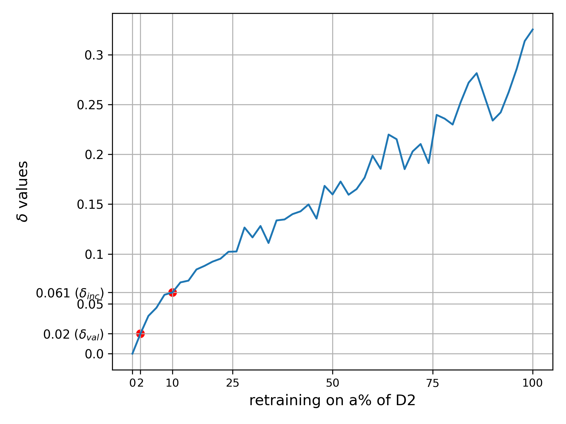
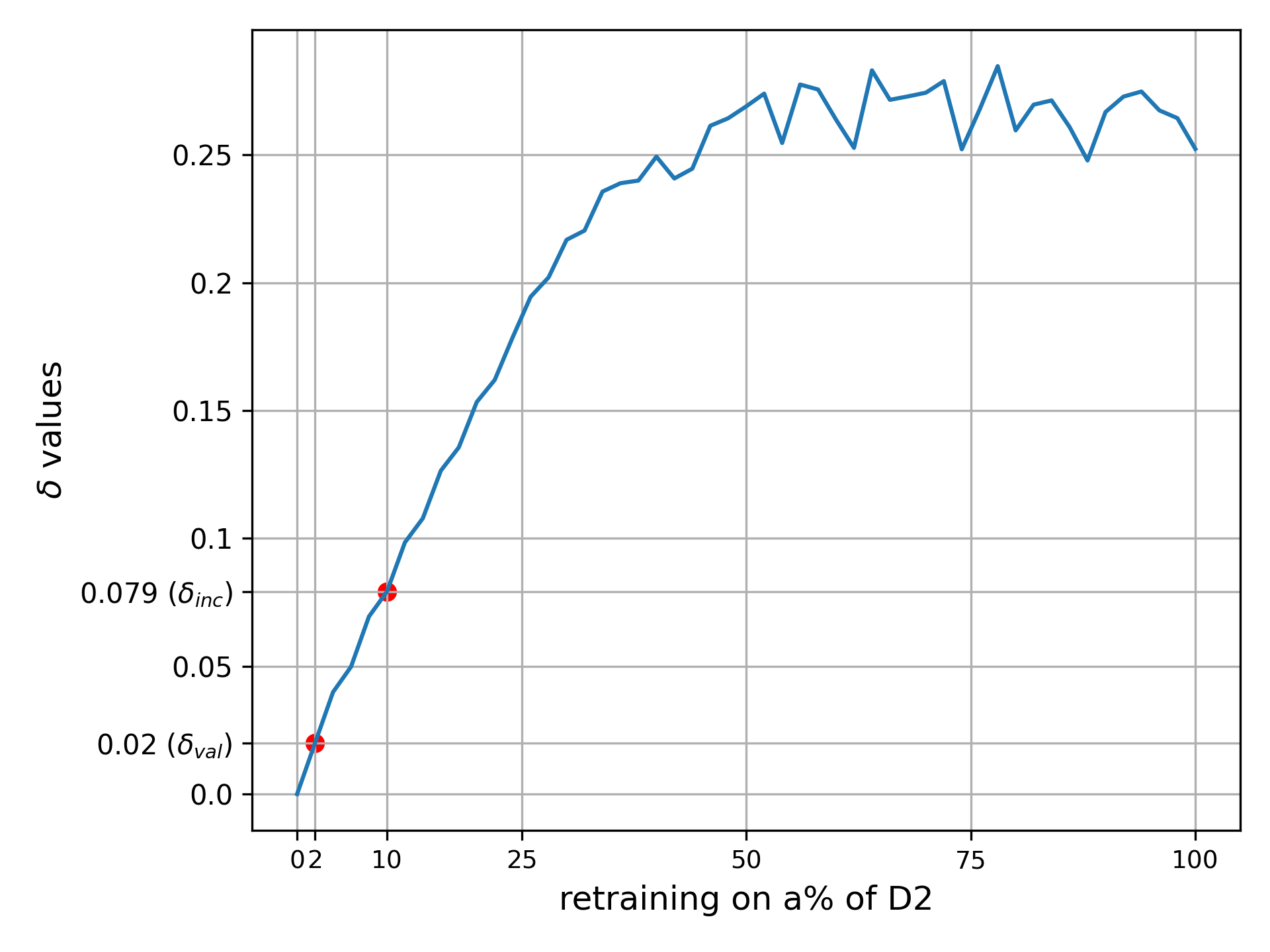
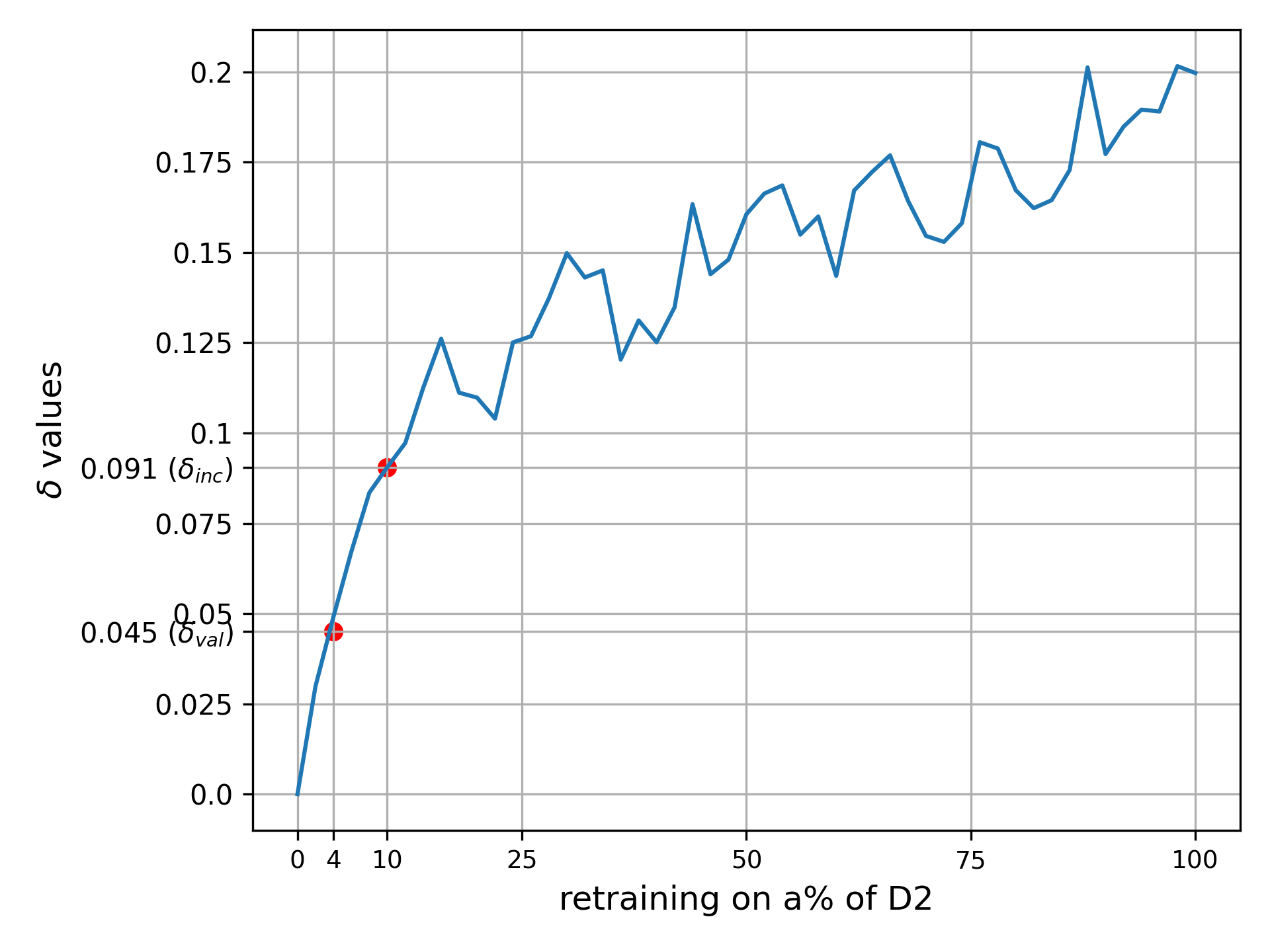
Recall from Definition 5 that upper-bounds the magnitude, measured in p-distance, of the model shifts in (Eq. 5). When practically using -robustness, , values, regarded as the hyperparameter in our method, need to be first determined. We now propose two realistic strategies for obtaining values, depending on how the underlying classifier is retrained with new data in the application.
Incremental retraining
This refers to the case where is periodically fine-tuned by gradient descent on some portions of with a small number of iterations. In this scenario, depending on how many data points in are used for retraining, the magnitude of parameter changes could be small. Therefore, the values can be directly estimated by calculating the p-distance between and the updated classifiers. By observing the p-distances when retraining on various portions of , the model developers could potentially link the estimated values to time intervals in real-world applications, depending on how quickly new data are collected.
Complete or leave-one-out retraining
Complete retraining means retraining a model with the same hyperparameter setting using the concatenation of and . Leave-one-out retraining concerns obtaining a new model using a subset of with 1% of data points removed. As mentioned in Hamman et al. (2023), when retraining from scratch using the concatenation of and , it becomes unrealistic to upper-bound the weights and biases differences in classifiers as the p-distance can be arbitrarily large. In this case, we can treat as a hyperparameter and empirically find the optimal target. Similarly to the standard train-validation-test split for evaluating the accuracy of machine learning models, we propose to use a held-out validation set to estimate values which lead to sufficient robustness under such retraining scenarios. The procedures are as follows:
-
1.
Retrain from scratch some new classifiers using and 444Complete retraining is possible in an experimental environment. In practice, however, if is not available at the time of robust CE generation, leave-one-out retraining on could be a viable option in step 1., set initial value to a sufficiently small value,
-
2.
Generate -robust CEs using the current .
-
3.
Evaluate the percentage of the explanations which are valid under all the retrained models.
-
4.
Examine the above empirical validity, if it has not reached 100% then increase the value and repeat steps 2-3. Choose the smallest value which results in 100% validity.
The terminating condition in step 4 balances the robustness-cost tradeoff. Once the empirical validity on multiple retrained models reaches 100% for the validation set, increasing further will negatively affect the proximity evaluations. It is also expected that when finding -robust CEs with the same value for the test set, a similar level of robustness can be observed.
We report the value results using both strategies in Figure 4, referred to as (incremental retraining) and (validation set). Specifically, for the first scenario, we record and plot values as the average -distances (in the experiments, we use ) between and five incrementally retrained555We reimplemented the partial_fit function in Scikit-learn library. models using increasing sizes of the retraining dataset (a% of ). As can be observed, values increase with slight fluctuations as incrementally retraining on more data. The magnitudes are classifier- and dataset-dependent, though in our setting we obtain values from 0 to about 0.3. The values are obtained by recording the values when retraining on of , and use them as one robustness target in the next experiments.
For the second scenario, we use five completely retrained and five leave-one-out retrained classifiers as the new models in Step 1. We use RNCE-FF to find -robust CEs in Step 2. We record the obtained as another robustness target, and we highlight these values in the same plots in Figure 4. After matching their magnitudes to the ones obtained for incremental retraining, we identify that these are much smaller than and they correspond to the magnitudes of retraining on only 2% of . The fact that being -robust against a very small magnitude results in 100% empirical robustness (validity) in a validation set confirms the conservative nature of -robustness, as it guarantees the CE’s robustness against all possible model shifts entailed by (Lemma 2).

8.3 Verifying -Robustness

In this experiment, we demonstrate how -robustness can be used as an evaluation tool to examine the robustness of CEs.
CEs are generated using the following SOTA algorithms. We consider three traditional non-robust baselines, namely a gradient-descent based method GCE similar to Wachter et al. (2017), a plausible method using gradient descent Proto Van Looveren and Klaise (2021), and a MILP-based method (referred to as MCE) inspired by Mohammadi et al. (2021). We also include ROAR Upadhyay et al. (2021), a SOTA framework specifically designed to generate robust CEs, focusing on robustness against the same notion of plausible model changes666Differently to our previous work Jiang et al. (2023a), we use the implementation of ROAR in CARLA library Pawelczyk et al. (2021) which allows more comprehensive hyperparameter tuning.. For our algorithms, using the iterative algorithm (Algorithm 1) proposed in Section 7, we devise robustified versions of the non-robust baselines, which we call GCE-R, PROTO-R, and MCE-R, to demonstrate the effectiveness of Algorithm 1 for improving robustness. We also include our RNCE-FF algorithm (Algorithm 2, robustInit=False, optimal=False) to show the guaranteed robustness results of this method.
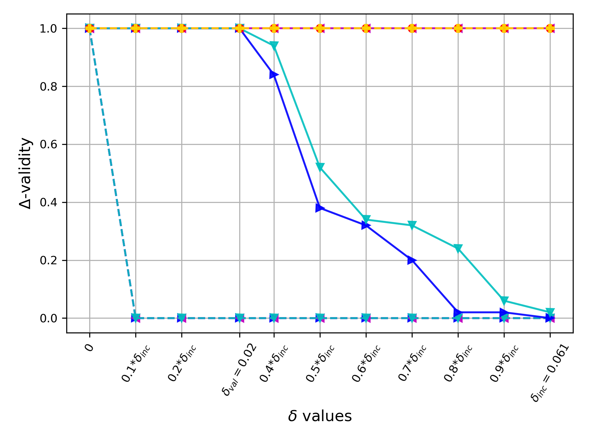
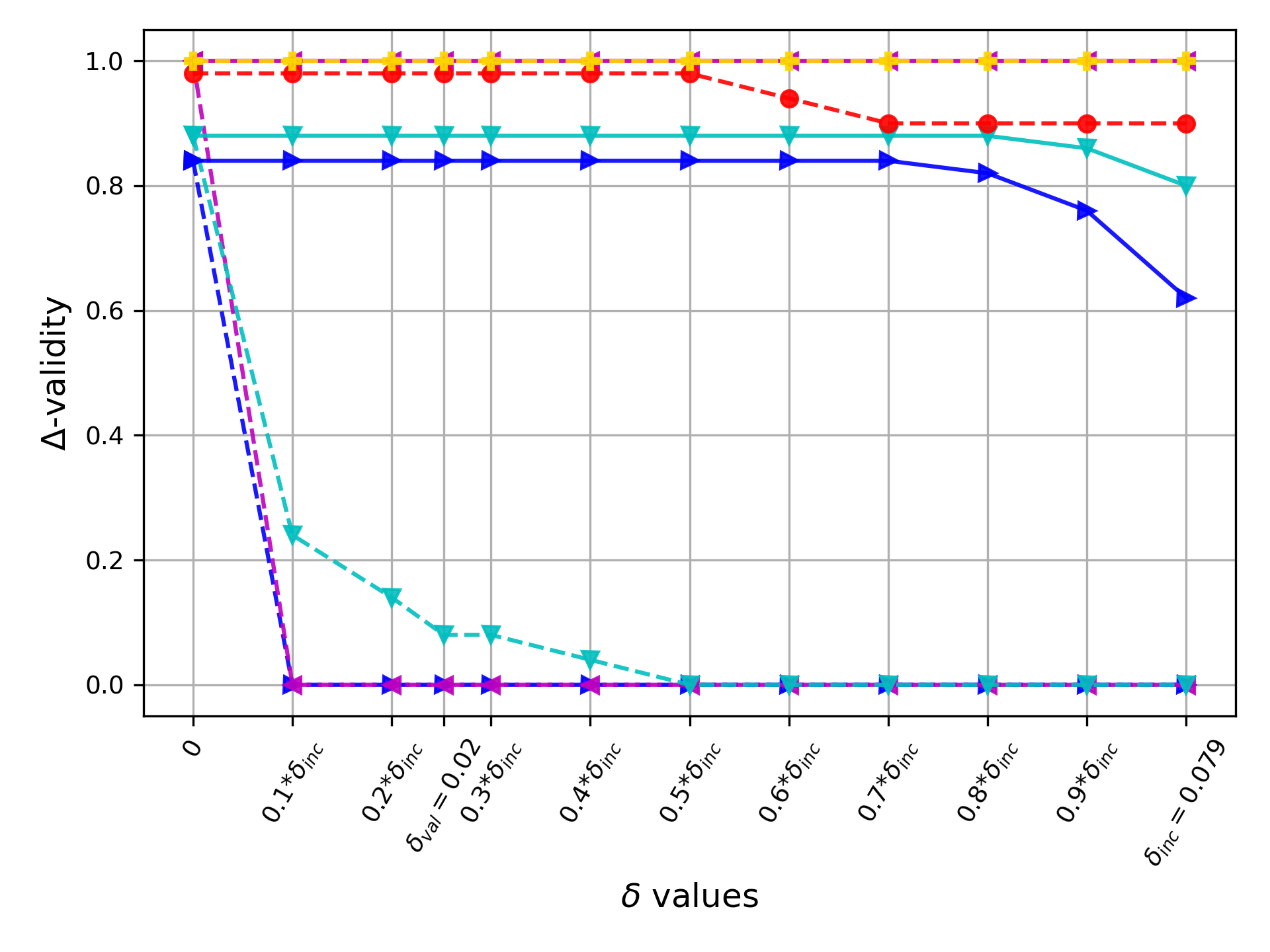
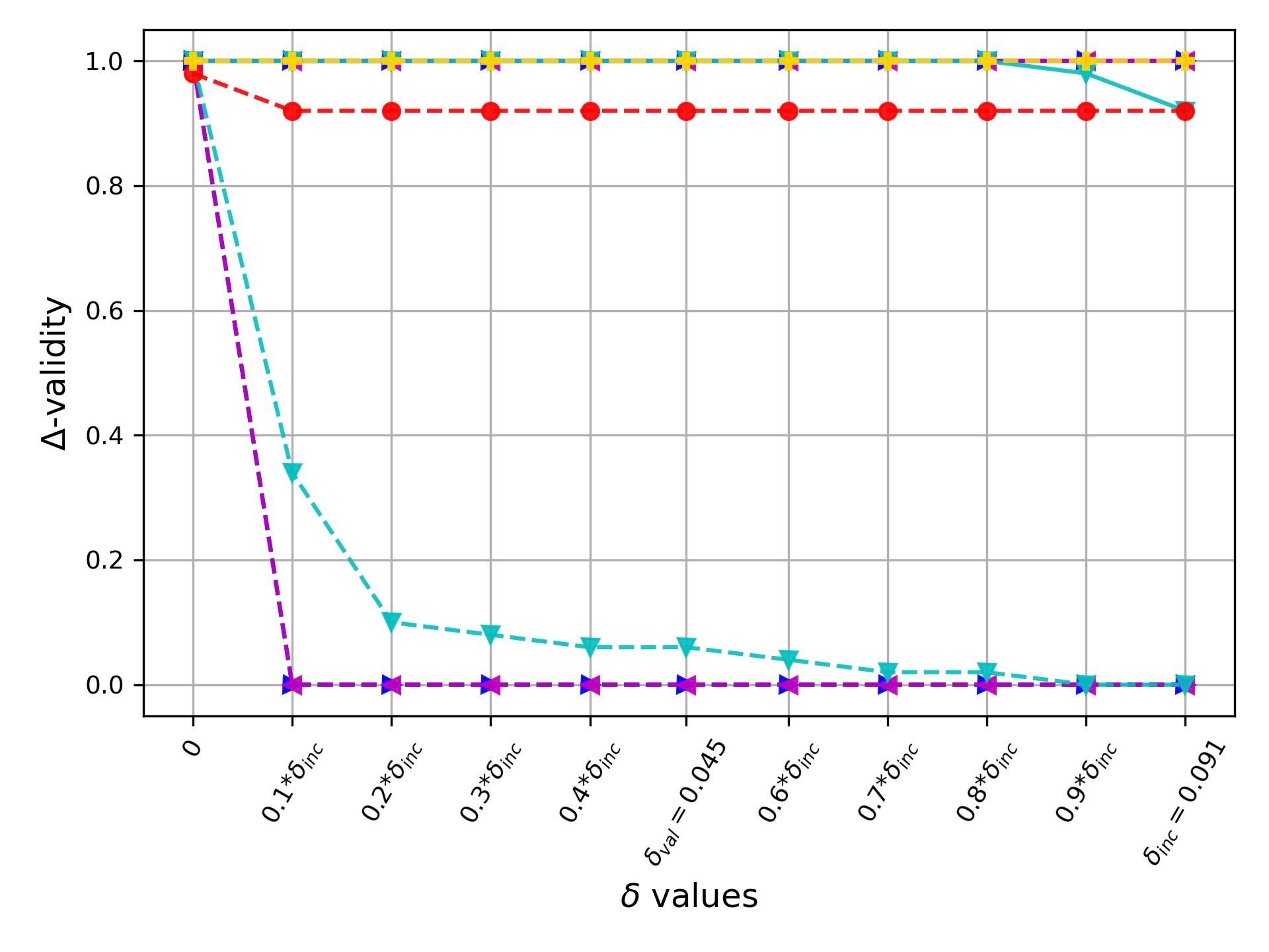
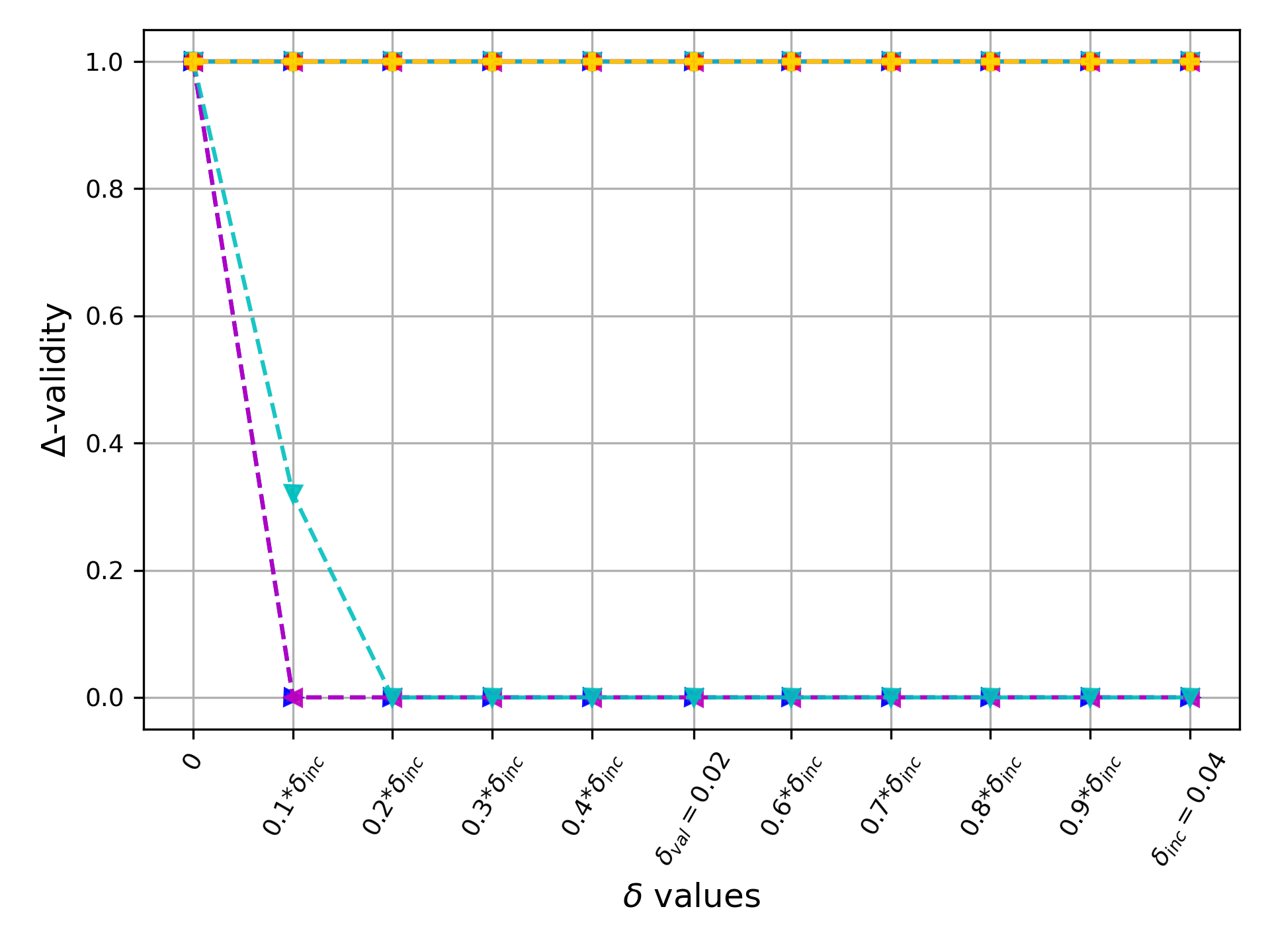
For each dataset, we randomly select 50 test inputs for which we use the above baselines to generate CEs. We evaluate their robustness against model shifts of magnitudes up to using -validity, the percentage of test inputs whose CEs are -robust. For all robust methods, their targeted values are instantiated with .
Figures 5 (a-d) report the results of our analysis for the four datasets. As we can observe, all methods generate CEs that tend to be valid for the original model. For the non-robust baselines, -validities soon drop to value 0 as small model shifts are applied, revealing a lack of robustness for these baselines. ROAR exhibits a higher degree of -robustness, as expected. However, its heuristic nature does not allow to reason about all possible shifts in , which affects the -robustness of CFXs as grows larger. Also, the fact that it uses a local surrogate model to approximate the behaviour of neural networks could negatively affect the results. For compas and gmc datasets, its -robustness stays lower than 100%.
For the two gradient-based non-robust baselines, our robustified versions (GCE-R, PROTO-R) successfully improved their robustness against small model shifts with lower values, however, the -robustness tends to drop (drastically for adult dataset) when it increases near . This is likely due to the vulnerability to local optimum solutions for the gradient-descent algorithms. The MILP-based method MCE-R which gives more exact solutions for the problem always finds robust CEs with 100% -validity. With proven robustness guarantees, our RNCE algorithm also finds CEs that are 100% robust.
8.4 Generating -robust CEs
| Method | Properties | Classifiers | ||||
| Validity | Proximity | Plausibility | Robustness | NN | LR | |
| GCE Wachter et al. (2017) | ||||||
| PROTO Van Looveren and Klaise (2021) | ||||||
| MCE Mohammadi et al. (2021) | ||||||
| NNCE Brughmans et al. (2023) | ||||||
| RBR Nguyen et al. (2022) | ||||||
| ROAR Upadhyay et al. (2021) | ||||||
| ST-CE Dutta et al. (2022) | ||||||
| GCE-R (ours) | ||||||
| PROTO-R (ours) | ||||||
| MCE-R (ours) | ||||||
| RNCE (ours) | ||||||
| vr | v | v | lof | vr | v | v | lof | |||
| adult | compas | |||||||||
| GCE | 51% | 0% | 0% | .016 | 1.29 | 26.5% | 0% | 0% | .039 | 3.05 |
| PROTO | 61.1% | 1% | 0% | .011 | 1.44 | 50.7% | 6.6% | 0% | .144 | 1.66 |
| MCE | 48.5% | 0% | 0% | .009 | 1.41 | 25.6% | 0% | 0% | .019 | 1.79 |
| NNCE | 76.1% | 2% | 2% | .032 | 1.34 | 43.3% | 8% | 0% | .028 | 1.30 |
| ROAR | 100% | 100% | 94.8% | .877 | 12.5 | 100% | 100% | 94.7% | .388 | 8.44 |
| RBR | 90.1% | 0% | 0% | .025 | 1.33 | 98.3% | 38% | 0% | .038 | 1.53 |
| ST-CE | 98.7% | 20% | 4% | .046 | 1.27 | 99.9% | 74% | 0% | .039 | 1.23 |
| target | target | |||||||||
| GCE-R | 100% | 100% | 0% | .048 | 1.47 | 86.9% | 87% | 0% | .055 | 3.04 |
| PROTO-R | 100% | 69% | 0% | .042 | 1.68 | 91% | 91% | 0% | .049 | 1.74 |
| MCE-R | 100% | 100% | 0% | .021 | 1.65 | 99.8% | 100% | 0% | .035 | 1.68 |
| RNCE-FF | 100% | 100% | 4% | .057 | 1.32 | 100% | 100% | 0% | .039 | 1.26 |
| RNCE-FT | 100% | 100% | 0% | .049 | 1.28 | 100% | 100% | 0% | .037 | 1.33 |
| target | target | |||||||||
| GCE-R | 100% | 100% | 0% | .051 | 1.65 | 87% | 87% | 67% | .109 | 3.62 |
| PROTO-R | 100% | 100% | 9% | .072 | 2.36 | 91% | 91% | 84% | .108 | 1.99 |
| MCE-R | 100% | 100% | 100% | .051 | 2.91 | 100% | 100% | 100% | .096 | 2.81 |
| RNCE-FF | 100% | 100% | 100% | .122 | 2.78 | 100% | 100% | 100% | .088 | 1.11 |
| RNCE-FT | 100% | 100% | 100% | .095 | 2.70 | 100% | 100% | 100% | .088 | 1.11 |
| gmc | heloc | |||||||||
| GCE | 75.8% | 0% | 0% | .022 | 1.52 | 20.5% | 0% | 0% | .019 | 1.18 |
| PROTO | 89.1% | 1% | 0% | .023 | 1.36 | 39.5% | 0% | 0% | .024 | 1.16 |
| MCE | 63.3% | 0% | 0% | .016 | 1.40 | 22% | 0% | 0% | .014 | 1.40 |
| NNCE | 88.9% | 22% | 1% | .029 | 1.23 | 35.9% | 0% | 0% | .053 | 1.05 |
| ROAR | 99.3% | 98% | 98% | .199 | 23.1 | 100% | 100% | 100% | .454 | 6.94 |
| RBR | 100% | 62% | 0% | .034 | 1.55 | 58.7% | 0% | 0% | .038 | 1.08 |
| ST-CE | 100% | 92% | 6% | .041 | 1.10 | 100% | 40% | 0% | .078 | 1.04 |
| target | target | |||||||||
| GCE-R | 100% | 100% | 0% | .032 | 1.79 | 100% | 100% | 0% | .049 | 1.32 |
| PROTO-R | 100% | 100% | 0% | .036 | 1.45 | 100% | 100% | 11% | .079 | 1.62 |
| MCE-R | 100% | 100% | 0% | .022 | 1.48 | 100% | 100% | 0% | .031 | 1.94 |
| RNCE-FF | 100% | 100% | 7% | .040 | 1.07 | 100% | 100% | 0% | .083 | 1.04 |
| RNCE-FT | 100% | 100% | 0% | .035 | 1.36 | 100% | 100% | 0% | .080 | 1.04 |
| target | target | |||||||||
| GCE-R | 100% | 100% | 100% | .053 | 3.43 | 100% | 100% | 100% | .109 | 2.07 |
| PROTO-R | 100% | 100% | 100% | .118 | 2.49 | 100% | 100% | 100% | .163 | 2.41 |
| MCE-R | 100% | 100% | 100% | .032 | 1.86 | 100% | 100% | 100% | .049 | 3.04 |
| RNCE-FF | 100% | 100% | 100% | .084 | 1.22 | 100% | 100% | 100% | .150 | 1.13 |
| RNCE-FT | 100% | 100% | 100% | .084 | 1.22 | 100% | 100% | 100% | .150 | 1.13 |
Next, we rigorously benchmark the performance of our CE generation methods against various robust and non-robust baselines. Apart from the CE methods used in Section 8.3, we additionally include NNCE Brughmans et al. (2023), RBR Nguyen et al. (2022), and ST-CE Hamman et al. (2023). We refer to Section 2 for their details. We also instantiate RNCE-FT as one of our methods. The properties of all compared methods are summarised in Table 2.
For each dataset, we randomly select 20 test points from the test set to generate CEs using each method. We repeat the process five times with different random seeds and report the mean and standard deviation of the results. The CEs are evaluated against three aspects using the standard metrics in the literature. For proximity, we calculate the average cost between the test input and its CE, which captures both closeness of CEs and sparsity of changes Wachter et al. (2017). For plausibility, we report the average local outlier factor score lof Breunig et al. (2000) which quantifies the local data density. A lof score close to value 1 indicates an inlier; the more it deviates from 1, the less plausible the CE. For robustness, we report validity after retraining vr, i.e. the percentage of CEs correctly classified to class 1, under 15 retrained classifiers using respectively complete retraining, leave-one-out retraining, and incremental retraining (with 10% new data). We use the same and obtained from Section 8.2 to instantiate with different model shift magnitudes and report the respective -robustness, termed v and v.
Table 3 reports the mean results for neural network classifiers of the benchmarking study. See B for the standard deviation results and the evaluations for logistic regression classifiers. Next, we analyse the results by their properties, and for our methods, we first consider the results when targeting .
Our methods produce the most robust CEs
Our RNCE algorithm (both configurations) generates the most robust CEs among the compared methods, showing 100% vr and 100% targeted -validity. For the robustified methods using Algorithm 2, MCE-R is the most robust, finding perfectly -robust and 100% empirically robust CEs in most experiments. As discussed in Section 8.3, the limited search space might be the cause of the reduced robustness for GCE-R and PROTO-R in two datasets. As a result, when compared with the robust baselines, RNCE and MCE-R both give better robustness than ROAR, ST-CE, and RBR. All robust methods have better robustness performances than the non-robust baselines, as expected.
Cost-robustness tradeoff
This tradeoff has been discussed in several other studies Upadhyay et al. (2021); Pawelczyk et al. (2023a), which we have also empirically observed. The non-robust baselines always find the most proximal CEs (lowest costs). Apart from them, the next best proximity results were obtained by MCE-R (when targeting the smaller ) among all the robust methods. Considering that MCE-R also finds near-perfectly -robust CEs, it can be concluded that MCE-R effectively balances the cost-robustness tradeoff. RBR also finds CEs with low costs, but their method is not as robust. Similar remarks can be made for ST-CE as this method moves more towards the robustness end of the tradeoff. Our methods GCE-R, PROTO-R, RNCE demonstrate similar costs. Setting optimal=True in our RNCE algorithm slightly improves the proximity, as can be seen when comparing RNCE-FF and RNCE-FT. ROAR results in CEs with high cost, and the method has been identified as being overly costly Nguyen et al. (2023) due to their gradient-based robust optimisation procedure.
Plausibility results
ST-CE have the best lof scores among all the methods while the results from RNCE are comparable, this is because these two methods select in-manifold dataset points as the resulting CEs and thus are unlikely to return outliers. By inherently addressing data density estimation, RBR also finds plausible CEs. The plausibility performances of our three robustified methods and ROAR are not as good due to less regulated search spaces or lack of plausibility constraints, with ROAR having the worst lof results.
The effects of robustification
For Algorithm 1, robustifying GCE, PROTO, and MCE resulted in improved empirical and robustness, but this negatively affected the proximity and plausibility results. Targeting larger-magnitude plausible model shifts (instantiated with ) pushes these tradeoffs further. For RNCE, similar trends can be identified when compared with NNCE, but in most cases, the lof score improves. When targeting instead of , the cost also increases together with robustness, but plausibility stays comparable.
Concluding remarks
From the analysis above, we can conclude that MCE-R achieved the best robustness-cost tradeoff, finding the most proximal CEs among the robust baselines while showing near-perfect robustness results, outperforming all robust baselines. RNCE, on the other hand, finds CEs with even stronger robustness guarantees and great plausibility, at slightly higher costs. However, any less-costly methods than RNCE are not as robust.
8.5 Multi-Class Classification
| Dataset | Method | vr | v | lof | |
|---|---|---|---|---|---|
| iris | NNCE | 75% | 0% | .393 | 1.48 |
| RNCE-FF | 100% | 100% | .438 | 1.50 | |
| RNCE-FT | 100% | 100% | .438 | 1.50 | |
| housing | NNCE | 18.1% | 0% | .032 | 1.10 |
| RNCE-FF | 100% | 100% | .053 | 1.33 | |
| RNCE-FT | 100% | 100% | .052 | 1.31 |
Next, we demonstrate the applicability of our RNCE method to multi-class classification settings, which is not supported by any robust CE generation baselines listed in Table 2. We use the Iris dataset Anderson (1936); Fisher (1936), a small-scale dataset for three-class classification tasks, and the California Housing dataset Pace and Barry (1997), in which we transform the regression labels into three classes. Both datasets are available in sklearn Pedregosa et al. (2011). We trained neural network models with cross validation accuracies 0.93 and 0.70. Again, we randomly select (five times with different random seeds) 20 test instances from the test sets which are classified to class 0, and we specify a desired label 2 for CEs. Following similar experimental procedures in Section 8.4, we use the validation set strategy to identify values as our targeted plausible model changes magnitude, and we report the same evaluation metrics for NNCE and RNCE.
Table 8.5 presents the final evaluations. Similarly to the results for binary classification, the CEs computed by the NNCE method are not robust against realistically retrained models (indicated by the low vr). Measured by the -validity, they also fail to satisfy the -robustness tests for multi-class classifications. With a slight tradeoff with costs and lof scores, our two configurations of RNCE are both able to find perfectly robust CEs in this study. This demonstrates that the -robustness notion can be used to evaluate provable robustness guarantees for CEs, and our proposed algorithms succeed at finding more robust CEs in the multi-class classification setting.
9 Conclusion
Despite the recent advances in achieving robustness against model changes for CEs, we identified a key limitation in the current state-of-the-art, namely the lack of formal robustness guarantees. By introducing a novel interval abstraction technique and a novel notion, -robustness, we provided the first method in the literature to obtain CEs with provable robustness. We showed how such -robustness can be practically tested in binary and multi-class classification settings by solving optimisation problems via MILP, and we defined this process as -robustness tests. Further, two algorithms have been proposed to generate CEs that are provably -robust. To demonstrate how our methods can be used in reality, two strategies for identifying the appropriate hyperparameter in our method have been investigated, linking to three model retraining strategies. We then presented an extensive empirical evaluation involving eleven algorithms for generating CEs, including six algorithms specifically designed to generate robust explanations. Our results show that our MCE-R algorithm finds CEs with the lowest costs along with the best robustness results, and our RNCE outperforms existing approaches and is able to generate CEs that are both provably robust and plausible, achieving a balance in the robustness-cost and plausibility-cost tradeoffs. We see these outcomes as important contributions towards complementing existing formal approaches for XAI and making them applicable in practice.
This work opens up several promising avenues for future work. One such direction is to investigate relaxed forms of robustness, e.g., when the output intervals in for different classes overlap, with similar interval abstraction techniques. In this work, we considered the deterministic robustness guarantees, aiming at ensuring CEs’ validity against even worst-case model parameter perturbations encoded by . However, as a limitation of our approach, this notion is conservative in that, if not targeting adversarial attack scenarios, the worst-case perturbations might not always occur in realistic model retraining. As a result, the -robust CEs might be overly robust than needed. One potential way to overcome this is to determine the hyperparameter which controls the magnitude of model changes in using a validation set, as illustrated in Section 8.2. However, that requires additional computational efforts. Therefore, probabilistic relaxations of our -robustness notion allowing more fine-grained analyses would be valuable.
Another possibility is to investigate the -robustness of CEs under causal settings. CEs which conform to some structural causal models are usually within data distribution, and they reflect the true causes of predictions, making causality a desirable property Karimi et al. (2020, 2021). It has also been found that plausible CEs are likely to be more robust against model shifts Pawelczyk et al. (2020b). Therefore, there could be intrinsic links between causality and robustness. Dominguez-Olmedo et al. (2022) have proposed a framework to compute CEs robust to noisy executions under a causal setting. It would be interesting to also investigate the interplay of -robustness and causality to facilitate the development of higher-quality CEs.
Finally, it would be possible to apply similar interval abstraction techniques to provide robustness guarantees for other forms of CE robustness. In our -robustness tests, a fixed-value CE is fed into the interval-valued abstraction of a classification model. Intuitively, if instead an interval-valued CE is passed as input into a fixed-valued classification model, it would be similar to reasoning about the robustness of CEs against noisy executions. Going further, it would be interesting to investigate training techniques incorporating -robustness notions to train models which can produce robust CEs by plain gradient-based optimisation methods.
Acknowledgements
Jiang, Rago and Toni were partially funded by J.P. Morgan and by the Royal Academy of Engineering under the Research Chairs and Senior Research Fellowships scheme. The authors acknowledge financial support from Imperial College London through an Imperial College Research Fellowship grant awarded to Leofante. Rago and Toni were partially funded by the European Research Council (ERC) under the European Union’s Horizon 2020 research and innovation programme (grant agreement No. 101020934). Any views or opinions expressed herein are solely those of the authors listed.
References
- Albini et al. [2020] Emanuele Albini, Antonio Rago, Pietro Baroni, and Francesca Toni. Relation-based counterfactual explanations for bayesian network classifiers. In Proceedings of the 29th International Joint Conference on AI, IJCAI, pages 451–457, 2020.
- Anderson [1936] Edgar Anderson. The species problem in iris. Annals of the Missouri Botanical Garden, 23(3):457–509, 1936.
- Angwin et al. [2016] Surya Mattu Julia Angwin, Jeff Larson, and Lauren Kirchner. Machine bias: There’s software used across the country to predict future criminals. and it’s biased against blacks, 2016.
- Augustin et al. [2022] Maximilian Augustin, Valentyn Boreiko, Francesco Croce, and Matthias Hein. Diffusion visual counterfactual explanations. In Advances in Neural Information Processing Systems 35, NeurIPS, 2022.
- Bajaj et al. [2021] Mohit Bajaj, Lingyang Chu, Zi Yu Xue, Jian Pei, Lanjun Wang, Peter Cho-Ho Lam, and Yong Zhang. Robust counterfactual explanations on graph neural networks. In Advances in Neural Information Processing Systems 34, NeurIPS, pages 5644–5655, 2021.
- Black et al. [2022] Emily Black, Zifan Wang, and Matt Fredrikson. Consistent counterfactuals for deep models. In The 10th International Conference on Learning Representations, ICLR, 2022.
- Breunig et al. [2000] Markus M. Breunig, Hans-Peter Kriegel, Raymond T. Ng, and Jörg Sander. LOF: identifying density-based local outliers. In The 2000 ACM SIGMOD International Conference on Management of Data, pages 93–104, 2000.
- Brughmans et al. [2023] Dieter Brughmans, Pieter Leyman, and David Martens. Nice: an algorithm for nearest instance counterfactual explanations. Data mining and knowledge discovery, pages 1–39, 2023.
- Bui et al. [2022] Ngoc Bui, Duy Nguyen, and Viet Anh Nguyen. Counterfactual plans under distributional ambiguity. In The 10th International Conference on Learning Representations, ICLR, 2022.
- Carlini and Wagner [2017] Nicholas Carlini and David A. Wagner. Towards evaluating the robustness of neural networks. In IEEE Symposium on Security and Privacy, SP, pages 39–57, 2017.
- Celar and Byrne [2023] Lenart Celar and Ruth M. J. Byrne. How people reason with counterfactual and causal explanations for AI decisions in familiar and unfamiliar domains. Memory & Cognition, 51(7):1481–1496, 2023.
- Cukierski [2011] Will Cukierski. Give me some credit, 2011.
- Dandl et al. [2020] Susanne Dandl, Christoph Molnar, Martin Binder, and Bernd Bischl. Multi-objective counterfactual explanations. In 16th International Conference on Parallel Problem Solving from Nature, pages 448–469, 2020.
- Delaney et al. [2021] Eoin Delaney, Derek Greene, and Mark T. Keane. Instance-based counterfactual explanations for time series classification. In The 29th International conference on case-based reasoning, volume 12877 of Lecture Notes in Computer Science, pages 32–47, 2021.
- Dhurandhar et al. [2018] Amit Dhurandhar, Pin-Yu Chen, Ronny Luss, Chun-Chen Tu, Pai-Shun Ting, Karthikeyan Shanmugam, and Payel Das. Explanations based on the missing: Towards contrastive explanations with pertinent negatives. In Advances in Neural Information Processing Systems 31, NeurIPS, pages 590–601, 2018.
- Dominguez-Olmedo et al. [2022] Ricardo Dominguez-Olmedo, Amir-Hossein Karimi, and Bernhard Schölkopf. On the adversarial robustness of causal algorithmic recourse. In Proceedings of the 39th International Conference on Machine Learning, ICML 2022, volume 162 of PMLR, pages 5324–5342, 2022.
- Dua et al. [2017] Dheeru Dua, Casey Graff, et al. Uci machine learning repository. 2017.
- Dutta et al. [2022] Sanghamitra Dutta, Jason Long, Saumitra Mishra, Cecilia Tilli, and Daniele Magazzeni. Robust counterfactual explanations for tree-based ensembles. In Proceedings of the 39th International Conference on Machine Learning, ICML, volume 162 of PMLR, pages 5742–5756, 2022.
- Ferrario and Loi [2022] Andrea Ferrario and Michele Loi. The robustness of counterfactual explanations over time. IEEE Access, 10:82736–82750, 2022.
- FICO [2018] FICO. Explainable machine learning challenge, 2018.
- Fisher [1936] Ronald A Fisher. The use of multiple measurements in taxonomic problems. Annals of eugenics, 7(2):179–188, 1936.
- Gowal et al. [2019] Sven Gowal, Krishnamurthy Dvijotham, Robert Stanforth, Rudy Bunel, Chongli Qin, Jonathan Uesato, Relja Arandjelovic, Timothy Arthur Mann, and Pushmeet Kohli. Scalable verified training for provably robust image classification. In IEEE/CVF International Conference on Computer Vision, ICCV, pages 4841–4850, 2019.
- Guidotti [2022] Riccardo Guidotti. Counterfactual explanations and how to find them: literature review and benchmarking. Data Mining and Knowledge Discovery, pages 1–55, 2022.
- Guo et al. [2023] Hangzhi Guo, Feiran Jia, Jinghui Chen, Anna Cinzia Squicciarini, and Amulya Yadav. Rocoursenet: Robust training of a prediction aware recourse model. In Proceedings of the 32nd ACM International Conference on Information and Knowledge Management, CIKM, pages 619–628, 2023.
- Hamman et al. [2023] Faisal Hamman, Erfaun Noorani, Saumitra Mishra, Daniele Magazzeni, and Sanghamitra Dutta. Robust counterfactual explanations for neural networks with probabilistic guarantees. In Proceedings of the 40th International Conference on Machine Learning, ICML, volume 202 of PMLR, pages 12351–12367, 2023.
- Henriksen and Lomuscio [2023] Patrick Henriksen and Alessio Lomuscio. Robust training of neural networks against bias field perturbations. In Brian Williams, Yiling Chen, and Jennifer Neville, editors, The 37th AAAI Conference on Artificial Intelligence, AAAI, pages 14865–14873, 2023.
- Jiang et al. [2023a] Junqi Jiang, Francesco Leofante, Antonio Rago, and Francesca Toni. Formalising the robustness of counterfactual explanations for neural networks. In The 37th AAAI Conference on Artificial Intelligence, AAAI, pages 14901–14909, 2023.
- Jiang et al. [2023b] Junqi Jiang, Antonio Rago, Francesco Leofante, and Francesca Toni. Recourse under model multiplicity via argumentative ensembling. arXiv preprint arXiv:2312.15097, 2023.
- Jiang et al. [2024a] Junqi Jiang, Jianglin Lan, Francesco Leofante, Antonio Rago, and Francesca Toni. Provably robust and plausible counterfactual explanations for neural networks via robust optimisation. In Proceedings of the 15th Asian Conference on Machine Learning, ACML, volume 222 of PMLR, pages 582–597, 2024.
- Jiang et al. [2024b] Junqi Jiang, Francesco Leofante, Antonio Rago, and Francesca Toni. Robust counterfactual explanations in machine learning: A survey. arXiv preprint arXiv:2402.01928, 2024.
- Kanamori et al. [2020] Kentaro Kanamori, Takuya Takagi, Ken Kobayashi, and Hiroki Arimura. DACE: distribution-aware counterfactual explanation by mixed-integer linear optimization. In Proceedings of the 29th International Joint Conference on Artificial Intelligence, IJCAI, pages 2855–2862, 2020.
- Karimi et al. [2020] Amir-Hossein Karimi, Bodo Julius von Kügelgen, Bernhard Schölkopf, and Isabel Valera. Algorithmic recourse under imperfect causal knowledge: a probabilistic approach. In Advances in Neural Information Processing Systems 33, NeurIPS, 2020.
- Karimi et al. [2021] Amir-Hossein Karimi, Bernhard Schölkopf, and Isabel Valera. Algorithmic recourse: from counterfactual explanations to interventions. In FAccT 2021: ACM Conference on Fairness, Accountability, and Transparency, pages 353–362, 2021.
- Karimi et al. [2023] Amir-Hossein Karimi, Gilles Barthe, Bernhard Schölkopf, and Isabel Valera. A survey of algorithmic recourse: Contrastive explanations and consequential recommendations. ACM Comput. Surv., 55(5):95:1–95:29, 2023.
- Krishna et al. [2023] Satyapriya Krishna, Jiaqi Ma, and Himabindu Lakkaraju. Towards bridging the gaps between the right to explanation and the right to be forgotten. In Proceedings of the 40th International Conference on Machine Learning, ICML, volume 202 of PMLR, pages 17808–17826, 2023.
- Leofante and Lomuscio [2023a] Francesco Leofante and Alessio Lomuscio. Robust explanations for human-neural multi-agent systems with formal verification. In Proceedings of the 20th European Conference on Multi-Agent Systems, EUMAS, volume 14282 of Lecture Notes in Computer Science, pages 244–262, 2023.
- Leofante and Lomuscio [2023b] Francesco Leofante and Alessio Lomuscio. Towards robust contrastive explanations for human-neural multi-agent systems. In Proceedings of the 22nd International Conference on Autonomous Agents and Multiagent Systems, AAMAS, pages 2343–2345, 2023.
- Leofante and Potyka [2024] Francesco Leofante and Nico Potyka. Promoting counterfactual robustness through diversity. In The 38th AAAI Conference on Artificial Intelligence, AAAI (to appear), 2024.
- Leofante et al. [2023] Francesco Leofante, Elena Botoeva, and Vineet Rajani. Counterfactual explanations and model multiplicity: a relational verification view. In Proceedings of the 20th International Conference on Principles of Knowledge Representation and Reasoning, KR, pages 763–768, 2023.
- Lomuscio and Maganti [2017] Alessio Lomuscio and Lalit Maganti. An approach to reachability analysis for feed-forward relu neural networks. arXiv preprint arXiv:1706.07351, 2017.
- Maragno et al. [2024] Donato Maragno, Jannis Kurtz, Tabea E Röber, Rob Goedhart, Ş Ilker Birbil, and Dick den Hertog. Finding regions of counterfactual explanations via robust optimization. INFORMS Journal on Computing, 2024.
- Marques-Silva and Ignatiev [2022] João Marques-Silva and Alexey Ignatiev. Delivering trustworthy AI through formal XAI. In The 36th AAAI Conference on Artificial Intelligence, pages 12342–12350, 2022.
- Miller [2019] Tim Miller. Explanation in artificial intelligence: Insights from the social sciences. Artif. Intell., 267:1–38, 2019.
- Mirman et al. [2018] Matthew Mirman, Timon Gehr, and Martin T. Vechev. Differentiable abstract interpretation for provably robust neural networks. In Proceedings of the 35th International Conference on Machine Learning, ICML, volume 80 of PMLR, pages 3575–3583, 2018.
- Mishra et al. [2021] Saumitra Mishra, Sanghamitra Dutta, Jason Long, and Daniele Magazzeni. A survey on the robustness of feature importance and counterfactual explanations. arXiv preprint arXiv:2111.00358, 2021.
- Mohammadi et al. [2021] Kiarash Mohammadi, Amir-Hossein Karimi, Gilles Barthe, and Isabel Valera. Scaling guarantees for nearest counterfactual explanations. In AIES ’21: AAAI/ACM Conference on AI, Ethics, and Society, pages 177–187, 2021.
- Mothilal et al. [2020] Ramaravind Kommiya Mothilal, Amit Sharma, and Chenhao Tan. Explaining machine learning classifiers through diverse counterfactual explanations. In FAT* 2020: ACM Conference on Fairness, Accountability, and Transparency, pages 607–617, 2020.
- Nguyen et al. [2022] Tuan-Duy H. Nguyen, Ngoc Bui, Duy Nguyen, Man-Chung Yue, and Viet Anh Nguyen. Robust bayesian recourse. In Proceedings of the 38th Conference on Uncertainty in Artificial Intelligence, volume 180 of PMLR, pages 1498–1508, 2022.
- Nguyen et al. [2023] Duy Nguyen, Ngoc Bui, and Viet Anh Nguyen. Distributionally robust recourse action. In The 11th International Conference on Learning Representations, ICLR, 2023.
- Pace and Barry [1997] R Kelley Pace and Ronald Barry. Sparse spatial autoregressions. Statistics & Probability Letters, 33(3):291–297, 1997.
- Pawelczyk et al. [2020a] Martin Pawelczyk, Klaus Broelemann, and Gjergji Kasneci. Learning model-agnostic counterfactual explanations for tabular data. In WWW ’20: The Web Conference 2020, pages 3126–3132, 2020.
- Pawelczyk et al. [2020b] Martin Pawelczyk, Klaus Broelemann, and Gjergji Kasneci. On counterfactual explanations under predictive multiplicity. In Proceedings of the 36th Conference on Uncertainty in Artificial Intelligence, UAI, volume 124 of PMLR, pages 809–818, 2020.
- Pawelczyk et al. [2021] Martin Pawelczyk, Sascha Bielawski, Johannes van den Heuvel, Tobias Richter, and Gjergji Kasneci. CARLA: A python library to benchmark algorithmic recourse and counterfactual explanation algorithms. In NeurIPS Datasets and Benchmarks track, 2021.
- Pawelczyk et al. [2023a] Martin Pawelczyk, Teresa Datta, Johannes van den Heuvel, Gjergji Kasneci, and Himabindu Lakkaraju. Probabilistically robust recourse: Navigating the trade-offs between costs and robustness in algorithmic recourse. In The 11th International Conference on Learning Representations, ICLR, 2023.
- Pawelczyk et al. [2023b] Martin Pawelczyk, Tobias Leemann, Asia Biega, and Gjergji Kasneci. On the trade-off between actionable explanations and the right to be forgotten. In The 11th International Conference on Learning Representations, ICLR, 2023.
- Pedregosa et al. [2011] F. Pedregosa, G. Varoquaux, A. Gramfort, V. Michel, B. Thirion, O. Grisel, M. Blondel, P. Prettenhofer, R. Weiss, V. Dubourg, J. Vanderplas, A. Passos, D. Cournapeau, M. Brucher, M. Perrot, and E. Duchesnay. Scikit-learn: Machine learning in Python. JMLR, 12:2825–2830, 2011.
- Prabhakar and Afzal [2019] Pavithra Prabhakar and Zahra Rahimi Afzal. Abstraction based output range analysis for neural networks. In Advances in Neural Information Processing Systems 32, NeurIPS, pages 15762–15772, 2019.
- Rawal et al. [2020] Kaivalya Rawal, Ece Kamar, and Himabindu Lakkaraju. Algorithmic recourse in the wild: Understanding the impact of data and model shifts. arXiv preprint arXiv:2012.11788, 2020.
- Slack et al. [2021] Dylan Slack, Anna Hilgard, Himabindu Lakkaraju, and Sameer Singh. Counterfactual explanations can be manipulated. In Advances in Neural Information Processing Systems 34, NeurIPS, pages 62–75, 2021.
- Tolomei et al. [2017] Gabriele Tolomei, Fabrizio Silvestri, Andrew Haines, and Mounia Lalmas. Interpretable predictions of tree-based ensembles via actionable feature tweaking. In Proceedings of the 23rd ACM SIGKDD International Conference on Knowledge Discovery and Data Mining, pages 465–474, 2017.
- Tsai et al. [2021] Yu-Lin Tsai, Chia-Yi Hsu, Chia-Mu Yu, and Pin-Yu Chen. Formalizing generalization and adversarial robustness of neural networks to weight perturbations. In Advances in Neural Information Processing Systems 34, NeurIPS, pages 19692–19704, 2021.
- Upadhyay et al. [2021] Sohini Upadhyay, Shalmali Joshi, and Himabindu Lakkaraju. Towards robust and reliable algorithmic recourse. In Advances in Neural Information Processing Systems 34, NeurIPS, pages 16926–16937, 2021.
- Ustun et al. [2019] Berk Ustun, Alexander Spangher, and Yang Liu. Actionable recourse in linear classification. In FAT* 2019: ACM Conference on Fairness, Accountability, and Transparency, pages 10–19, 2019.
- Van Looveren and Klaise [2021] Arnaud Van Looveren and Janis Klaise. Interpretable counterfactual explanations guided by prototypes. In Joint European Conference on Machine Learning and Knowledge Discovery in Databases, pages 650–665, 2021.
- Virgolin and Fracaros [2023] Marco Virgolin and Saverio Fracaros. On the robustness of sparse counterfactual explanations to adverse perturbations. Artif. Intell., 316:103840, 2023.
- Wachter et al. [2017] Sandra Wachter, Brent D. Mittelstadt, and Chris Russell. Counterfactual explanations without opening the black box: Automated decisions and the GDPR. Harv. JL & Tech., 31:841, 2017.
- Weng et al. [2018] Tsui-Wei Weng, Huan Zhang, Pin-Yu Chen, Jinfeng Yi, Dong Su, Yupeng Gao, Cho-Jui Hsieh, and Luca Daniel. Evaluating the robustness of neural networks: An extreme value theory approach. In The 6th International Conference on Learning Representations, ICLR, 2018.
- Weng et al. [2020] Tsui-Wei Weng, Pu Zhao, Sijia Liu, Pin-Yu Chen, Xue Lin, and Luca Daniel. Towards certificated model robustness against weight perturbations. In The 34th AAAI Conference on Artificial Intelligence, AAAI, pages 6356–6363, 2020.
- Wong and Kolter [2018] Eric Wong and J. Zico Kolter. Provable defenses against adversarial examples via the convex outer adversarial polytope. In Proceedings of the 35th International Conference on Machine Learning, ICML, volume 80 of PMLR, pages 5283–5292, 2018.
- Zhang et al. [2020] Huan Zhang, Hongge Chen, Chaowei Xiao, Sven Gowal, Robert Stanforth, Bo Li, Duane S. Boning, and Cho-Jui Hsieh. Towards stable and efficient training of verifiably robust neural networks. In The 8th International Conference on Learning Representations, ICLR, 2020.
Appendices
Appendix A Computation Time of RNCE and the Impact of robustInit
Since querying for the nearest neighbour from a k-d tree is in logarithm time complexity wrt the tree size, the computation time bottleneck of RNCE is the total time for the more complex -robustness tests. Therefore, the computation time of RNCE mainly depends on two factors, the time required for each -robustness test, and the number of -robustness tests performed in total. For the former factor, each -robustness test is a MILP program whose problem size, affected by the number of attributes in the dataset and the architecture of the classifier in our setting, determines its computation time. The latter factor, however, is directly controlled by the algorithm parameter, robustInit. When robustInitF, the number of -robustness tests is the product of the number of inputs for which CEs are generated and the average number of times querying for the next nearest neighbour (Alg.3, lines 4-6) before reaching a -robust CE, which is further affected by the value of constructing . When robustInitT, the number of -robustness tests is upper-bounded by the dataset size.
We empirically compare the computation time when robustInitT with robustInitF. Specifically, since the line search controlled by the parameter optimal (Alg. 4, lines 7-10) is independent of the impact of robustInit, we report results for optimalF, i.e., RNCE-FF and RNCE-TF, under two different settings, in Tables 5 and 6.
| configuration | adult | compas | gmc | heloc | ||||
|---|---|---|---|---|---|---|---|---|
| NN | LR | NN | LR | NN | LR | NN | LR | |
| RNCE-FF | 7.69 | 0.47 | 11.47 | 4.34 | 4.33 | 0.41 | 55.83 | 0.49 |
| RNCE-TF incl. time for obtaining | 59.55 | 3.84 | 20.21 | 1.77 | 268.35 | 43.20 | 44.23 | 3.17 |
| RNCE-TF excl. time for obtaining | 0.002 | 0.002 | 0.001 | 0.001 | 0.008 | 0.007 | 0.001 | 0.002 |
| Configuration | adult (15500) | compas (200) | gmc (700) | heloc (2000) | ||||
|---|---|---|---|---|---|---|---|---|
| NN | LR | NN | LR | NN | LR | NN | LR | |
| RNCE-FF | 1306 | 59.55 | 27.16 | 5.63 | 42.44 | 1.22 | 1052 | 9.79 |
| RNCE-TF incl. time for obtaining | 59.75 | 4.15 | 20.21 | 1.77 | 268.42 | 43.21 | 44.24 | 3.19 |
| RNCE-TF excl. time for obtaining | 0.21 | 0.31 | 0.001 | 0.001 | 0.08 | 0.02 | 0.01 | 0.02 |
The results empirically support our analysis. The computation times of both RNCE-TF and RNCE-FF for neural networks are much higher than those for logistic regressions due to the fact that neural networks are more complex in terms of model architecture. The computation time of RNCE-FF tends to be lower than RNCE-TF when the number of inputs is smaller because fewer -robustness tests are required. When robustInitF, the time is almost proportional to the number of inputs. When robustInitT, the computation times are almost identical regardless of the number of inputs because building the k-d tree is more time-consuming than querying for CEs. Our RNCE-TF excl. time for obtaining results show that, when robustInitT, after obtaining , the time needed for querying CEs is almost negligible, since for every input, the first query will be the closest -robust CE.
Appendix B Full Experiment Results
| vr | v | v | lof | vr | v | v | lof | |||
| adult | compas | |||||||||
| GCE | .223 | 0 | 0 | .003 | .036 | .011 | 0 | 0 | .007 | .697 |
| PROTO | .178 | .020 | 0 | .002 | .089 | .172 | .055 | 0 | .062 | .192 |
| MCE | .201 | 0 | 0 | .001 | .063 | .126 | 0 | 0 | .006 | .047 |
| NNCE | .139 | .024 | .024 | .004 | .114 | .123 | .024 | 0 | .003 | .057 |
| ROAR | 0 | 0 | .065 | .208 | 4.187 | 0 | 0 | .033 | .033 | .574 |
| RBR | .092 | 0 | 0 | .002 | .051 | .008 | .024 | 0 | .003 | .170 |
| ST-CE | .014 | .071 | .020 | .008 | .087 | .003 | .128 | 0 | .003 | .057 |
| target | target | |||||||||
| GCE-R | 0 | 0 | 0 | .007 | .079 | .041 | .040 | 0 | .006 | .664 |
| PROTO-R | 0 | .203 | 0 | .010 | .119 | .037 | .037 | 0 | .008 | .299 |
| MCE-R | 0 | 0 | 0 | .001 | .099 | .002 | 0 | 0 | .003 | .161 |
| RNCE-FF | 0 | 0 | .020 | .005 | .021 | 0 | 0 | 0 | .003 | .062 |
| RNCE-FT | 0 | 0 | 0 | .003 | .045 | 0 | 0 | 0 | .003 | .060 |
| target | target | |||||||||
| GCE-R | 0 | 0 | 0 | .008 | .130 | .040 | .040 | .051 | .005 | .565 |
| PROTO-R | 0 | 0 | .091 | .053 | .356 | .037 | .037 | .058 | .009 | .244 |
| MCE-R | 0 | 0 | 0 | .005 | .054 | 0 | 0 | 0 | .004 | .235 |
| RNCE-FF | 0 | 0 | 0 | .006 | .168 | 0 | 0 | 0 | .004 | .086 |
| RNCE-FT | 0 | 0 | 0 | .011 | .085 | 0 | 0 | 0 | .004 | .086 |
| gmc | heloc | |||||||||
| GCE | .003 | 0 | 0 | .005 | .064 | .042 | 0 | 0 | .002 | .045 |
| PROTO | .012 | .020 | 0 | .004 | .057 | .052 | 0 | 0 | .002 | .036 |
| MCE | .032 | 0 | 0 | .003 | .103 | .053 | 0 | 0 | .001 | .034 |
| NNCE | .027 | .068 | .020 | .003 | .031 | .053 | 0 | 0 | .003 | .011 |
| ROAR | .015 | .025 | .025 | .014 | 9.69 | 0 | 0 | 0 | .010 | .164 |
| RBR | 0 | .117 | 0 | .004 | .105 | .070 | 0 | 0 | .003 | .022 |
| ST-CE | 0 | .087 | .058 | .005 | .068 | 0 | .152 | 0 | .004 | .016 |
| target | target | |||||||||
| GCE-R | 0 | 0 | 0 | .006 | .019 | 0 | 0 | 0 | .003 | .043 |
| PROTO-R | 0 | 0 | 0 | .004 | .019 | 0 | 0 | .073 | .002 | .061 |
| MCE-R | 0 | 0 | 0 | .003 | .103 | .002 | 0 | 0 | .001 | .043 |
| RNCE-FF | 0 | 0 | .087 | .004 | .033 | 0 | 0 | 0 | .002 | .019 |
| RNCE-FT | 0 | 0 | 0 | .004 | .157 | 0 | 0 | 0 | .003 | .019 |
| target | target | |||||||||
| GCE-R | 0 | 0 | 0 | .006 | .021 | 0 | 0 | 0 | .010 | .114 |
| PROTO-R | 0 | 0 | 0 | .011 | .014 | 0 | 0 | 0 | .003 | .025 |
| MCE-R | 0 | 0 | 0 | .003 | .100 | 0 | 0 | 0 | .002 | .055 |
| RNCE-FF | 0 | 0 | 0 | .007 | .036 | 0 | 0 | 0 | .003 | .022 |
| RNCE-FT | 0 | 0 | 0 | .007 | .036 | 0 | 0 | 0 | .003 | .022 |
| vr | v | v | lof | vr | v | v | lof | |||
| adult | compas | |||||||||
| NNCE | 97.9% | 45% | 42% | .078 | 1.99 | 73.6% | 1% | 49% | .034 | 1.32 |
| ROAR | 100% | 100% | 100% | .265 | 1.69 | 100% | 100% | 96.8% | .220 | 2.59 |
| target | target | |||||||||
| RNCE-FF | 100% | 100% | 70% | .085 | 2.21 | 100% | 100% | 100% | .045 | 1.22 |
| RNCE-FT | 100% | 100% | 16% | .060 | 1.71 | 100% | 100% | 100% | .043 | 1.30 |
| target | target | |||||||||
| RNCE-FF | 100% | 100% | 100% | .087 | 2.18 | 86.1% | 1% | 100% | .035 | 1.30 |
| RNCE-FT | 100% | 100% | 100% | .064 | 1.74 | 78.1% | 0% | 100% | .033 | 1.34 |
| gmc | heloc | |||||||||
| NNCE | 92.7% | 57% | 51% | .035 | 1.21 | 77.5% | 5% | 49% | .057 | 1.06 |
| ROAR | 100% | 100% | 100% | .119 | 2.76 | 100% | 100% | 100% | .089 | 1.42 |
| target | target | |||||||||
| RNCE-FF | 100% | 100% | 92% | .043 | 1.23 | 100% | 100% | 100% | .070 | 1.06 |
| RNCE-FT | 100% | 100% | 35% | .034 | 1.23 | 100% | 100% | 0% | .066 | 1.05 |
| target | target | |||||||||
| RNCE-FF | 100% | 100% | 100% | .043 | 1.17 | 98.8% | 10% | 100% | .061 | 1.06 |
| RNCE-FT | 100% | 100% | 100% | .035 | 1.23 | 96.7% | 0% | 100% | .054 | 1.06 |
| vr | v | v | lof | vr | v | v | lof | |||
| adult | compas | |||||||||
| NNCE | .035 | .130 | .144 | .017 | .188 | .025 | .020 | .037 | .003 | .068 |
| ROAR | 0 | 0 | 0 | .028 | .020 | 0 | 0 | 0 | .002 | .151 |
| target | target | |||||||||
| RNCE-FF | 0 | 0 | .122 | .016 | .251 | 0 | 0 | 0 | .003 | .032 |
| RNCE-FT | 0 | 0 | .092 | .010 | .070 | 0 | 0 | 0 | .002 | .060 |
| target | target | |||||||||
| RNCE-FF | 0 | 0 | 0 | .015 | .273 | .015 | .020 | 0 | .003 | .068 |
| RNCE-FT | 0 | 0 | 0 | .009 | .104 | .002 | 0 | 0 | .003 | .093 |
| gmc | heloc | |||||||||
| NNCE | .028 | .129 | .159 | .003 | .021 | .023 | .045 | .102 | .003 | .013 |
| ROAR | 0 | 0 | 0 | .010 | .225 | 0 | 0 | 0 | .003 | .038 |
| target | target | |||||||||
| RNCE-FF | 0 | 0 | .112 | .004 | .055 | 0 | 0 | 0 | .003 | .021 |
| RNCE-FT | 0 | 0 | .055 | .004 | .048 | 0 | 0 | 0 | .004 | .019 |
| target | target | |||||||||
| RNCE-FF | 0 | 0 | 0 | .003 | .039 | .010 | .008 | 0 | .003 | .016 |
| RNCE-FT | 0 | 0 | 0 | .004 | .053 | .012 | 0 | 0 | .004 | .015 |
For linear regression models, we find and using the same strategy for neural networks as stated in Section 8.2. We quantitatively compare the CEs found by NNCE, ROAR, and two configurations of our algorithm RNCE using the same evaluation metrics introduced in Section 8.4. Tables 8 and 9 report the mean and standard deviation results for logistic regression classifiers.
Slightly different from the neural network results, the values, found by incrementally retraining on 10% of , can be smaller than the , and sometimes insufficient to induce 100% empirical robustness (indicated by vr). Comparing RNCE with baselines, similar to the results for neural networks in Section 8.4, RNCE produces more robust CEs than the NNCE method, and is less costly and more plausible than ROAR. The impact of changing optimal to True is more obvious in this set of experiments, with costs decreasing to a greater extent and plausibility remaining comparable to RNCE-FF.