Elucidating the Design Space of Dataset Condensation

Abstract

Dataset condensation, a concept within data-centric learning, efficiently transfers critical attributes from an original dataset to a synthetic version, maintaining both diversity and realism. This approach significantly improves model training efficiency and is adaptable across multiple application areas. Previous methods in dataset condensation have faced challenges: some incur high computational costs which limit scalability to larger datasets (e.g., MTT, DREAM, and TESLA), while others are restricted to less optimal design spaces, which could hinder potential improvements, especially in smaller datasets (e.g., SRe²L, G-VBSM, and RDED). To address these limitations, we propose a comprehensive design framework that includes specific, effective strategies like implementing soft category-aware matching and adjusting the learning rate schedule. These strategies are grounded in empirical evidence and theoretical backing. Our resulting approach, Elucidate Dataset Condensation (EDC), establishes a benchmark for both small and large-scale dataset condensation. In our testing, EDC achieves state-of-the-art accuracy, reaching 48.6% on ImageNet-1k with a ResNet-18 model at an IPC of 10, which corresponds to a compression ratio of 0.78%. This performance exceeds those of SRe²L, G-VBSM, and RDED by margins of 27.3%, 17.2%, and 6.6%, respectively.

1 Introduction

Dataset condensation, also known as dataset distillation, has emerged in response to the ever-increasing training demands of advanced deep learning models [1, 2, 3]. This approach addresses the challenge of requiring high-precision models while also managing substantial resource constraints [4, 5, 6]. In this method, the original dataset acts as a “teacher”, distilling and preserving essential information into a smaller, surrogate “student” dataset. The ultimate goal of this technique is to achieve performance comparable to the original by training models from scratch with the condensed dataset. This approach has become popular in various downstream applications, including continual learning [7, 8, 9], neural architecture search [10, 11, 12], and training-free network slimming [13].

Unfortunately, the prohibitively expensive bi-level optimization paradigm limits the effectiveness of traditional dataset distillation methods, such as those presented in previous studies [14, 15, 16], particularly when applied to large-scale datasets like ImageNet-1k [17]. In response, the uni-level optimization paradigm has gained significant attention as a potential solution, with recent contributions from the research community [18, 19, 20] highlighting its utility. These methods primarily leverage the rich and extensive information from static, pre-trained observer models, facilitating a more streamlined optimization process on a condensed dataset without the need to adjust other parameters (e.g., those within the observer models). While uni-level optimization has demonstrated remarkable performance on large datasets, it has yet to achieve the benchmark accuracy levels seen with classical methods on datasets like CIFAR-10/100 [21]. Moreover, the newly developed training-free RDED [22] significantly outperforms previous methods in efficiency and maintains effectiveness, yet it overlooks the potential information loss due to the lack of image optimization. Additionally, some simple but promising techniques (e.g., smoothing the learning rate schedule) that could enhance performance have been underexplored in existing literature. For instance, applying these techniques allowed RDED to achieve a performance improvement of 16.2%.

These drawbacks show the constraints of previous methods in several respects, highlighting the need for a thorough investigation and assessment of these issues. In contrast to earlier strategies that targeted specific improvements, our approach systematically examines all viable facets and integrates them into our novel framework. To establish a comprehensive model, we carefully analyze deficiencies during the data synthesis, soft label generation, and post-evaluation stages of dataset condensation, resulting in an extensive exploration of the design space on the large-scale ImageNet-1k. As a result, we introduce Elucidate Dataset Condensation (EDC), which includes a range of detailed and effective enhancements (refer to Fig. 1). For instance, soft category-aware matching ( ) ensures consistent category representation between the original and condensed dataset batches for more precise matching. Importantly, EDC not only achieves state-of-the-art performance on CIFAR-10, CIFAR-100, Tiny-ImageNet, ImageNet-10, and ImageNet-1k, at half the computational expense compared to the baseline G-VBSM, but it also provides in-depth empirical and theoretical insights that affirm the soundness of our design decisions.

2 Dataset Condensation

Preliminary. Dataset condensation involves generating a synthetic dataset $\mathcal{D}^{\mathcal{S}}:=\{\mathbf{x}^{\mathcal{S}}_{i},\mathbf{y}^{\mathcal{S}}_{i}\}_{i=1}^{\lvert\mathcal{D}^{\mathcal{S}}\rvert}$ consisting of images $\mathcal{X}^{\mathcal{S}}$ and labels $\mathcal{Y}^{\mathcal{S}}$, designed to be as informative as the original dataset $\mathcal{D}^{\mathcal{T}}:=\{\mathbf{x}^{\mathcal{T}}_{i},\mathbf{y}^{\mathcal{T}}_{i}\}_{i=1}^{\lvert\mathcal{D}^{\mathcal{T}}\rvert}$, which includes images $\mathcal{X}^{\mathcal{T}}$ and labels $\mathcal{Y}^{\mathcal{T}}$. The synthetic dataset $\mathcal{D}^{\mathcal{S}}$ is substantially smaller in size than $\mathcal{D}^{\mathcal{T}}$ ($\lvert\mathcal{D}^{\mathcal{S}}\rvert\ll\lvert\mathcal{D}^{\mathcal{T}}\rvert$). The goal of this process is to maintain the critical attributes of $\mathcal{D}^{\mathcal{T}}$ to ensure robust or comparable performance during evaluations on test protocol $\mathcal{P}_{\mathcal{D}}$.

$$\operatorname{arg\,min}\mathbb{E}_{(\mathbf{x},\mathbf{y})\sim\mathcal{P}_{\mathcal{D}}}[\ell_{\textbf{{eval}}}(\mathbf{x},\mathbf{y},\phi^{*})],\ \ \textrm{where}\ \phi^{*}=\operatorname{arg\,min}_{\phi}\mathbb{E}_{(\mathbf{x}_{i}^{\mathcal{S}},\mathbf{y}_{i}^{\mathcal{S}})\sim\mathcal{D}^{\mathcal{S}}}[\ell(\phi(\mathbf{x}_{i}^{\mathcal{S}}),\mathbf{y}_{i}^{\mathcal{S}})].$$ (1)

Here, $\ell_{\textbf{{eval}}}(\cdot,\cdot,\phi^{*})$ represents the evaluation loss function, such as cross-entropy loss, which is parameterized by the neural network $\phi^{*}$ that has been optimized from the distilled dataset $\mathcal{D}^{\mathcal{S}}$. The data synthesis process primarily determines the quality of the distilled datasets, which transfers desirable knowledge from $\mathcal{D}^{\mathcal{T}}$ to $\mathcal{D}^{\mathcal{S}}$ through various matching mechanisms, such as trajectory matching [14], gradient matching [12], distribution matching [11] and generalized matching [20].

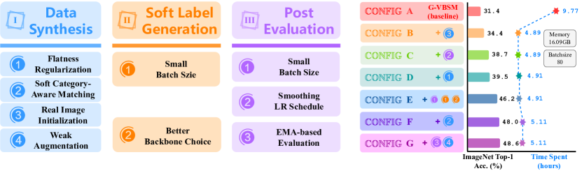
Figure 1: Illustration of Elucidating Dataset Condensation (EDC). Left: The overall of our better design choices in dataset condensation on ImageNet-1k. Right: The evaluation performance and data synthesis required time of different configurations on ResNet-18 with IPC 10. Our integral EDC refers to $\mathbb{C}\mathbb{O}\mathbb{N}\mathbb{F}\mathbb{I}\mathbb{G}$ G.

Small-scale vs. Large-scale Dataset Condensation/Distillation. Traditional dataset condensation algorithms, as referenced in studies such as [23, 14, 24, 25, 26], encounter computational challenges and are generally confined to small-scale datasets like CIFAR-10/100 [21], or larger datasets with limited class diversity, such as ImageNette [14] and ImageNet-10 [27]. The primary inefficiency of these methods stems from their reliance on a bi-level optimization framework, which involves alternating updates between the synthetic dataset and the observer model utilized for distillation. This approach not only heavily depends on the model but also limits the versatility of the distilled datasets in generalizing across different architectures. In contrast, the uni-level optimization strategy, noted for its efficiency and enhanced performance on the regular 224$\times$224 scale of ImageNet-1k in recent research [18, 20, 19], shows reduced effectiveness in smaller-scale datasets due to the many iterations required in the data synthesis process without a direct connection to actual data. Recent new methods in training-free distillation paradigms, such as in [22, 28], offer advancements in efficiency. Nevertheless, these methods compromise data privacy and do not leverage statistical information from observer models, thereby restraining their potential in a training-free environment.

Generalized Data Synthesis Paradigm. We consistently describe algorithms [18, 19, 20, 22] that efficiently conduct data synthesis on ImageNet-1k as “generalized data synthesis”. This approach avoids the inefficient bi-level optimization and includes both image and label synthesis phases. Specifically, generalized data synthesis involves initially generating highly condensed images followed by acquiring soft labels through predictions from a pre-trained model. The evaluation process resembles knowledge distillation [29], aiming to transfer knowledge from a teacher to a student model whenever feasible [30, 29]. The primary distinction between the training-dependent [18, 19, 20] and training-free paradigms [22] centers on their approach to data synthesis. In detail, the training-dependent paradigm employs Statistical Matching (SM) to extract pertinent information from the entire dataset.

$$\mathcal{L}_{\textbf{{syn}}} =||p(\mu|\mathcal{X}^{\mathcal{S}})-p(\mu|\mathcal{X}^{\mathcal{T}})||_{2}+||p(\sigma^{2}|\mathcal{X}^{\mathcal{S}})-p(\sigma^{2}|\mathcal{X}^{\mathcal{T}})||_{2},\ s.t.\ \mathcal{L}_{\textbf{{syn}}}\sim\mathbb{S}_{\textrm{match}},$$ (2)

$$\mathcal{X}^{\mathcal{S}*} =\operatorname*{arg\,min}_{\mathcal{X}^{\mathcal{S}}}\mathbb{E}_{\mathcal{L}_{\textbf{{syn}}}\sim\mathbb{S}_{\textrm{match}}}[\mathcal{L}_{\textbf{{syn}}}(\mathcal{X}^{\mathcal{S}},\mathcal{X}^{\mathcal{T}})],$$

where $\mathbb{S}_{\textrm{match}}$ represents the extensive collection of statistical matching operators, which operate across a variety of network architectures and layers as described by [20]. Here, $\mu$ and $\sigma^{2}$ are defined as the mean and variance, respectively. For more detailed theoretical insights, please refer to Definition 3.1. The training-free approach, as discussed in [22, 28], employs a direct reconstruction method for the original dataset, aiming to generate simplified representations of images.

$$\mathcal{X}^{\mathcal{S}}=\bigcup_{i=1}^{\mathbf{C}}\mathcal{X}^{\mathcal{S}}_{i},\ \mathcal{X}^{\mathcal{S}}_{i}=\{\mathbf{x}_{j}^{i}=\textrm{concat}(\{\tilde{\mathbf{x}}_{k}\}_{k=1}^{N}\subset\mathcal{X}^{\mathcal{T}}_{i})\}_{j=1}^{\mathsf{IPC}},$$ (3)

where $\mathbf{C}$ denotes the number of classes, $\textrm{concat}(\cdot)$ represents the concatenation operator, $\mathcal{X}^{\mathcal{S}}_{i}$ signifies the set of condensed images belonging to the $i$-th class, and $\mathcal{X}^{\mathcal{T}}_{i}$ corresponds to the set of original images of the $i$-th class. It is important to note that the default settings for $N$ are 1 and 4, as specified in the works [28] and [22], respectively. Using one or more observer models, denoted as $\{\phi_{i}\}_{i=1}^{N}$, we then derive the soft labels $\mathcal{Y}^{\mathcal{S}}$ from the condensed image set $\mathcal{X}^{\mathcal{S}}$.

$$\mathcal{Y}^{\mathcal{S}}=\bigcup_{\mathbf{x}_{i}^{\mathcal{S}}\subset\mathcal{X}^{\mathcal{S}}}\frac{1}{N}\sum_{i=1}^{N}\phi_{i}(\mathbf{x}_{i}^{\mathcal{S}}).$$ (4)

This plug-and-play component, as outlined in SRe²L [18] and IDC [27], plays a crucial role for enhancing the generalization ability of the distilled dataset $\mathcal{D}^{\mathcal{S}}$.

3 Improved Design Choices

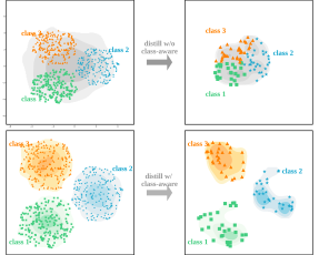
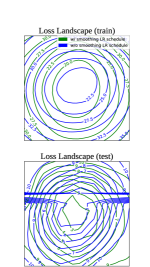
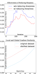
Figure 2: (a): Illustration of soft category-aware matching $\left(\vbox{\hbox{\includegraphics[height=10.33327pt]{figures/serial_number/data_synthesis_2.pdf}}}\right)$ using a Gaussian distribution in $\mathbb{R}^{2}$. (b): The effect of employing smoothing LR schedule $\left(\vbox{\hbox{\includegraphics[height=10.33327pt]{figures/serial_number/post_evaluation_2.pdf}}}\right)$ on loss landscape sharpness reduction. (c) top: The role of flatness regularization $\left(\vbox{\hbox{\includegraphics[height=10.33327pt]{figures/serial_number/data_synthesis_1.pdf}}}\right)$ in reducing the Frobenius norm of the Hessian matrix driven by data synthesis iteration. (c) bottom: Cosine similarity comparison between local gradients (obtained from original and distilled datasets via random batch selection) and the global gradient (obtained from gradient accumulation).

Design choices in data synthesis, soft label generation, and post-evaluation significantly influence the generalization capabilities of condensed datasets. Effective strategies for small-scale datasets are well-explored, yet these approaches are less examined for large-scale datasets. We first delineate the limitations of existing algorithms’ design choices on ImageNet-1k. We then propose solutions, showcasing experimental results as shown in Fig. 1. For most design choices, we offer both theoretical analysis and empirical insights to facilitate a thorough understanding, as detailed in Sec. 3.2.

3.1 Limitations of Prior Methods

Lacking Realism $\left(\text{solved by }\vbox{\hbox{\includegraphics[height=10.33327pt]{figures/serial_number/data_synthesis_3.pdf}}}\right)$. Training-dependent condensation algorithms for datasets, particularly those employed for large-scale datasets, typically initiate the optimization process using Gaussian noise inputs [18, 19, 20]. This initial choice complicates the optimization process and often results in the generation of synthetic images that do not exhibit high levels of realism. The limitations in visualization associated with previous approaches are detailed in Appendix F.

Coarse-grained Matching Mechanism $\left(\text{solved by }\vbox{\hbox{\includegraphics[height=10.33327pt]{figures/serial_number/data_synthesis_2.pdf}}}\right)$. The Statistical Matching (SM)-based pipeline [18, 19, 20] computes the global mean and variance by aggregating samples across all categories and uses these statistical parameters for matching purposes. However, this method exhibits two critical drawbacks: it does not account for the domain discrepancies among different categories, and it fails to preserve the integrity of category-specific information across the original and condensed samples within each batch. These limitations result in a coarse-grained matching approach that diminishes the accuracy of the matching process.

Overly Sharp of Loss Landscape $\left(\text{solved by }\vbox{\hbox{\includegraphics[height=10.33327pt]{figures/serial_number/data_synthesis_1.pdf}}}\ \text{and}\ \vbox{\hbox{\includegraphics[height=10.33327pt]{figures/serial_number/post_evaluation_3.pdf}}}\right)$. The optimization objective $\mathcal{L}(\theta)$ can be expanded through a second-order Taylor expansion as $\mathcal{L}(\theta^{*})+(\theta-\theta^{*})^{\mathrm{T}}\nabla_{\theta}\mathcal{L}(\theta^{*})+(\theta-\theta^{*})^{\mathrm{T}}\mathbf{H}(\theta-\theta^{*})$, with an upper bound of $\mathcal{L}(\theta^{*})+||\mathbf{H}||_{\mathbf{F}}\mathbb{E}[||\theta-\theta^{*}||_{2}^{2}]$ upon model convergence [31]. However, earlier training-dependent condensation algorithms neglect to minimize the Frobenius norm of the Hessian matrix $\mathbf{H}$ to obtain a flat loss landscape for enhancing its generalization capability through sharpness-aware minimization theory [32, 33]. Please see Appendix C for more formal information.

Irrational Hyperparameter Settings $\left(\text{solved by }\vbox{\hbox{\includegraphics[height=10.33327pt]{figures/serial_number/data_synthesis_4.pdf}}}\text{, }\vbox{\hbox{\includegraphics[height=10.33327pt]{figures/serial_number/soft_label_1.pdf}}}\text{, }\vbox{\hbox{\includegraphics[height=10.33327pt]{figures/serial_number/soft_label_2.pdf}}}\text{, }\vbox{\hbox{\includegraphics[height=10.33327pt]{figures/serial_number/post_evaluation_1.pdf}}}\ \text{and}\ \vbox{\hbox{\includegraphics[height=10.33327pt]{figures/serial_number/post_evaluation_2.pdf}}}\right)$. RDED [22] adopts a smoothing LR schedule $\left(\vbox{\hbox{\includegraphics[height=10.33327pt]{figures/serial_number/post_evaluation_2.pdf}}}\right)$ and [34, 19, 22] use a reduced batch size $\left(\vbox{\hbox{\includegraphics[height=10.33327pt]{figures/serial_number/post_evaluation_1.pdf}}}\vbox{\hbox{\includegraphics[height=10.33327pt]{figures/serial_number/soft_label_1.pdf}}}\right)$ for post-evaluation on the full 224$\times$224 ImageNet-1k. These changes, although critical, lack detailed explanations and impact assessments in the existing literature. Our empirical analysis highlights a remarkable impact on performance: absent these modifications, RDED achieves only 25.8% accuracy on ResNet18 with IPC 10. With these modifications, however, accuracy jumps to 42.0%. In contrast, SRe²L and G-VBSM do not incorporate such strategies in their experimental frameworks. This work aims to fill the gap by providing the first comprehensive empirical analysis and ablation study on the effects of these and similar improvements in the field.

3.2 Our Solutions

To address these limitations described previously, we explore the design space and elaborately present a range of optimal solutions at both empirical and theoretical levels, as illustrated in Fig. 1.

Figure 3: Comparison between real image initialization and random initialization.

Real Image Initialization $\left(\vbox{\hbox{\includegraphics[height=10.33327pt]{figures/serial_number/data_synthesis_3.pdf}}}\right)$. Intuitively, using real images instead of Gaussian noise for data initialization during the data synthesis phase is a practical and effective strategy. As shown in Fig. 3, this method significantly improves the realism of the condensed dataset and simplifies the optimization process, thus enhancing the synthesized dataset’s ability to generalize in post-evaluation tests. Additionally, we incorporate considerations of information density and efficiency by employing a training-free condensed dataset (typically via RDED) for initialization at the start of the synthesis process. According to Theorem 3.1, based on optimal transport theory, the cost of transporting from a Gaussian distribution to the original data distribution is higher than using the training-free condensed distribution as the initial reference. This advantage also allows us to reduce the number of iterations needed to achieve results to half of those required by our baseline G-VBSM model, significantly boosting synthesis efficiency.

Theorem 3.1.

(proof in Appendix B.1) Considering samples $\mathcal{X}^{\mathcal{S}}_{\textbf{{real}}}$, $\mathcal{X}^{\mathcal{S}}_{\textbf{{free}}}$, and $\mathcal{X}^{\mathcal{S}}_{\textbf{{random}}}$ from the original data, training-free condensed (e.g., RDED), and Gaussian distributions, respectively, let us assume a cost function defined in optimal transport theory that satisfies $\mathbb{E}[c(a-b)]\propto 1/I(\textrm{Law}(a),\textrm{Law}(b))$. Under this assumption, it follows that $\mathbb{E}[c(\mathcal{X}^{\mathcal{S}}_{\textbf{{real}}}-\mathcal{X}^{\mathcal{S}}_{\textbf{{free}}})]\leq\mathbb{E}[c(\mathcal{X}^{\mathcal{S}}_{\textbf{{real}}}-\mathcal{X}^{\mathcal{S}}_{\textbf{{random}}})]$.

Soft Category-Aware Matching $\left(\vbox{\hbox{\includegraphics[height=10.33327pt]{figures/serial_number/data_synthesis_2.pdf}}}\right)$. Previous dataset condensation methods [18, 19, 20] based on the Statistical Matching (SM) framework have shown satisfactory results predominantly when the data follows a unimodal distribution (e.g., a single Gaussian). This limitation is illustrated with a simple example in Fig. 2 (a). Typically, datasets consist of multiple classes with significant variations among their class distributions. Traditional SM-based methods compress data by collectively processing all samples, thus neglecting the differences between classes. As shown in the top part of Fig. 2 (a), this method enhances information density but also creates a big mismatch between the condensed source distribution $\mathcal{X}^{\mathcal{S}}$ and the target distribution $\mathcal{X}^{\mathcal{T}}$. To tackle this problem, we propose the use of a Gaussian Mixture Model (GMM) to effectively approximate any complex distribution. This solution is theoretically justifiable by the Tauberian Theorem under certain conditions (detailed proof provided in Appendix B.2). In light of this, we define two specific approaches to Statistical Matching:

Sketch Definition 3.1.

(formal definition in Appendix B.2) Given $N$ random samples $\{x_{i}\}_{i=1}^{N}$ with an unknown distribution $p_{\textrm{mix}}(x)$, we define two forms to statistical matching. Form (1): involves synthesizing $M$ distilled samples $\{y_{i}\}_{i=1}^{M}$, where $M\ll N$, ensuring that the variances and means of both $\{x_{i}\}_{i=1}^{N}$ and $\{y_{i}\}_{i=1}^{M}$ are consistent. Form (2): treats $p_{\textrm{mix}}(x)$ as a GMM with $\mathbf{C}$ components. For random samples $\{x_{i}^{j}\}_{i=1}^{N_{j}}$ ($\sum_{j}N_{j}=N$) within each component $c_{j}$, we synthesize $M_{j}$ ($\sum_{j}M_{j}=M$) distilled samples $\{y^{j}_{i}\}_{i=1}^{M_{j}}$, where $M_{j}\ll N_{j}$, to maintain the consistency of variances and means between $\{x^{j}_{i}\}_{i=1}^{N_{j}}$ and $\{y^{j}_{i}\}_{i=1}^{M_{j}}$.

In general, SRe²L, CDA, and G-VBSM are all categorized under Form (1), as shown in Fig. 2 (a) at the top, leading to coarse-grained matching. According to Fig. 2 (a) at the bottom, transitioning to Form (2) is identified as a practical and appropriate alternative. However, our empirical result indicates that exclusive reliance on Form (1) yields a synthesized dataset that lacks sufficient information density. Consequently, we propose for a hybrid method that effectively integrates Form (1) and Form (2) using a weighted average, which we term soft category-aware matching.

$$\mathcal{L}_{\textbf{{syn}}}^{\prime}=\alpha||p(\mu|\mathcal{X}^{\mathcal{S}})-p(\mu|\mathcal{X}^{\mathcal{T}})||_{2}+||p(\sigma^{2}|\mathcal{X}^{\mathcal{S}})-p(\sigma^{2}|\mathcal{X}^{\mathcal{T}})||_{2}{\color[rgb]{0.839216,0.152941,0.156863}\quad\#\textrm{Form (1)}}$$ (5)

$$+(1-\alpha)\sum_{i}^{\mathbf{C}}p(c_{i})\left[||p(\mu|\mathcal{X}^{\mathcal{S}},c_{i})-p(\mu|\mathcal{X}^{\mathcal{T}},c_{i})||_{2}+||p(\sigma^{2}|\mathcal{X}^{\mathcal{S}},c_{i})-p(\sigma^{2}|\mathcal{X}^{\mathcal{T}},c_{i})||_{2}\right],{\color[rgb]{0.839216,0.152941,0.156863}\quad\#\textrm{Form (2)}}$$

where $\mathbf{C}$ represents the total number of components, $c_{i}$ indicates the $i$-th component within a GMM, and $\alpha$ is a coefficient for adjusting the balance. The modified loss function $\mathcal{L}_{\textbf{{syn}}}^{\prime}$ is designed to effectively regulate the information density of $\mathcal{X}^{\mathcal{S}}$ and to align the distribution of $\mathcal{X}^{\mathcal{S}}$ with that of $\mathcal{X}^{\mathcal{T}}$. Operationally, each category in the original dataset is mapped to a distinct component in the GMM framework. Particularly, when $\alpha=1$, the sophisticated category-aware matching described by $\mathcal{L}_{\textbf{{syn}}}^{\prime}$ in Eq. 5 simplifies to the basic statistical matching defined by $\mathcal{L}_{\textbf{{syn}}}$ in Eq. 2.

Theorem 3.2.

(proofs in Theorems B.5, B.7, B.8 and Corollary B.6) Given the original data distribution $p_{\textrm{mix}}(x)$, and define condensed samples as $x$ and $y$ in Form (1) and Form (2) with their distributions characterized by $P$ and $Q$. Subsequently, it follows that (i) $\mathbb{E}[x]\equiv\mathbb{E}[y]$, (ii) $\mathbb{D}[x]\equiv\mathbb{D}[y]$, (iii) $\mathcal{H}(P)-\frac{1}{2}\left[\log(\mathbb{E}[\mathbb{D}[y^{j}]]+\mathbb{D}[\mathbb{E}[y^{j}]])-\mathbb{E}[\log(\mathbb{D}[y^{j}])]\right]\leq\mathcal{H}(Q)\leq\mathcal{H}(P)+\frac{1}{4}\mathbb{E}_{(i,j)\sim\prod[\mathbf{C},\mathbf{C}]}\left[\frac{(\mathbb{E}[y^{i}]-\mathbb{E}[y^{j}])^{2}(\mathbb{D}[y^{i}]+\mathbb{D}[y^{j}])}{\mathbb{D}[y^{i}]\mathbb{D}[y^{j}]}\right]$ and (iv) $D_{\textrm{KL}}[p_{\textrm{mix}}||P]\leq\mathbb{E}_{i\sim\mathcal{U}[1,\ldots,\mathbf{C}]}\mathbb{E}_{j\sim\mathcal{U}[1,\ldots,\mathbf{C}]}\frac{\mathbb{E}[y^{j}]^{2}}{\mathbb{D}[y^{i}]}$ and $D_{\textrm{KL}}[p_{\textrm{mix}}||Q]=0$.

We further analyze the properties of distributions $P$ and $Q$ as in Form (1) and Form (2). According to parts (i) and (ii) of Theorem 3.2, $Q$ retains the same variance and mean as $P$. Regarding diversity, part (iii) of Theorem 3.2 states that the entropy $\mathcal{H}(\cdot)$ of $P$ and $Q$ is equivalent, $\mathcal{H}(P)\equiv\mathcal{H}(Q)$, provided the mean and variance of all components in the GMM are uniform, suggesting a single Gaussian profile. Absent this condition, there is no guarantee that $\mathcal{H}(P)$ and $\mathcal{H}(Q)$ will consistently increase or decrease. These findings underscore the advantages of using GMM, especially when the initial data conforms to a unimodal distribution, thus aligning the mean, variance, and entropy of distributions $P$ and $Q$ in the reduced dataset. Moreover, even in diverse scenarios, the mean, variance, and entropy of $Q$ tend to remain stable. Furthermore, when the original dataset exhibits a more complex bimodal distribution and the parameters of the Gaussian components are precisely estimated, utilizing GMM can effectively reduce the Kullback-Leibler divergence between the mixed original distribution $p_{\textrm{mix}}$ and $Q$ to near zero. In contrast, the divergence $D_{\textrm{KL}}[p_{\textrm{mix}}||P]$ always maintains a non-zero upper bound, as noted in part (iv) of Theorem 3.2. Therefore, by modulating the weight $\alpha$ in Eq. 5, we can derive an optimally balanced solution that minimizes loss in data characteristics while maximizing fidelity between the synthesized and original distributions.

Flatness Regularization $\left(\vbox{\hbox{\includegraphics[height=10.33327pt]{figures/serial_number/data_synthesis_1.pdf}}}\right)$ and EMA-based Evaluation $\left(\vbox{\hbox{\includegraphics[height=10.33327pt]{figures/serial_number/post_evaluation_3.pdf}}}\right)$. Choices and are utilized to ensure flat loss landscapes during the stages of data synthesis and post-evaluation, respectively.

During the data synthesis phase, the use of sharpness-aware minimization (SAM) algorithms is beneficial for reducing the sharpness of the loss landscape, as presented in prior research [32, 35, 36]. Nonetheless, traditional SAM approaches, as detailed in Eq. 29 in the Appendix, generally double the computational load due to their two-stage parameter update process. This increase in computational demand is often impractical during data synthesis. Inspired by MESA [35], which achieves sharpness-aware training without additional computational overhead through self-distillation, we introduce a lightweight flatness regularization approach for implementing SAM during data synthesis. This method utilizes a teacher dataset, $\mathcal{X}_{\textbf{{EMA}}}^{\mathcal{S}}$, maintained via exponential moving average (EMA). The newly formulated optimization goal aims to foster a flat loss landscape in the following manner:

$$\mathcal{L}_{\textbf{{FR}}} =\mathbb{E}_{\mathcal{L}_{\textrm{syn}}\sim\mathbb{S}_{\textrm{match}}}[\mathcal{L}_{\textbf{{syn}}}(\mathcal{X}^{\mathcal{S}},\mathcal{X}^{\mathcal{S}}_{\textbf{{EMA}}})],\text{ }\mathcal{X}^{\mathcal{S}}_{\textbf{{EMA}}}=\beta\mathcal{X}^{\mathcal{S}}_{\textbf{{EMA}}}+(1-\beta)\mathcal{X}^{\mathcal{S}},$$ (6)

where $\beta$ is the weighting coefficient, which is empirically set to 0.99 in our experiments. The detail derivation of Eq. 7 is in Appendix E. And the critical theoretical result is articulated as follows:

Theorem 3.3.

(proof in Appendix E) The optimization objective $\mathcal{L}_{\textbf{{FR}}}$ can ensure sharpness-aware minimization within a $\rho$-ball for each point along a straight path between $\mathcal{X}^{\mathcal{S}}$ and $\mathcal{X}^{\mathcal{S}}_{\textbf{{EMA}}}$.

This indicates that the primary optimization goal of $\mathcal{L}_{\textbf{{FR}}}$ deviates somewhat from that of traditional SAM-based algorithms, which are designed to achieve a flat loss landscape around $\mathcal{X}^{\mathcal{S}}$. While both $\mathcal{L}_{\textbf{{FR}}}$ and conventional SAM-based methods are capable of performing sharpness-aware training, our findings unfortunately demonstrate that various SM-based loss functions do not converge to zero. This failure to converge contradicts the basic premise that the first-order term in the Taylor expansion should equal zero. As a result, we choose to apply flatness regularization exclusively to the logits of the observer model, since the cross-entropy loss for these can more straightforwardly reach zero.

$$\mathcal{L}^{\prime}_{\textbf{{FR}}} =D_{\textrm{KL}}(\textrm{softmax}(\phi(\mathcal{X}^{\mathcal{S}})/\tau)||\textrm{softmax}(\phi(\mathcal{X}^{\mathcal{S}}_{\textbf{{EMA}}})/\tau)),\text{ }\mathcal{X}^{\mathcal{S}}_{\textbf{{EMA}}}=\beta\mathcal{X}^{\mathcal{S}}_{\textbf{{EMA}}}+(1-\beta)\mathcal{X}^{\mathcal{S}},$$ (7)

where $\textrm{softmax}(\cdot)$, $\tau$ and $\phi$ represent the softmax operator, the temperature coefficient and the pre-trained observer model, respectively. As illustrated in Fig. 2 (c) top, it is evident that $\mathcal{L}^{\prime}_{\textbf{{FR}}}$ significantly lowers the Frobenius norm of the Hessian matrix relative to standard training, thus confirming its efficacy in pushing a flatter loss landscape.

In post-evaluation, we observe that a method analogous to $\mathcal{L}^{\prime}_{\textbf{{FR}}}$ employing SAM does not lead to appreciable performance improvements. This result is likely due to the limited sample size of the condensed dataset, which hinders the model’s ability to fully converge post-training, thereby undermining the advantages of flatness regularization. Conversely, the integration of an EMA-updated model as the validated model markedly stabilizes performance variations during evaluations. We term this strategy EMA-based evaluation and apply it across all benchmark experiments.

Dataset	IPC	ResNet-18				ResNet-50		ResNet-101		MobileNet-V2
		SRe2L	G-VBSM	RDED	EDC (Ours)	G-VBSM	EDC (Ours)	RDED	EDC (Ours)	EDC (Ours)
	1	-	-	22.9 $\pm$ 0.4	32.6 $\pm$ 0.1	-	30.6 $\pm$ 0.4	-	26.1 $\pm$ 0.2	20.2 $\pm$ 0.4
CIFAR-10	10	27.2 $\pm$ 0.4	53.5 $\pm$ 0.6	37.1 $\pm$ 0.3	79.1 $\pm$ 0.3	-	76.0 $\pm$ 0.3	-	67.1 $\pm$ 0.5	42.0 $\pm$ 0.4
	50	47.5 $\pm$ 0.5	59.2 $\pm$ 0.4	62.1 $\pm$ 0.1	87.0 $\pm$ 0.1	-	86.9 $\pm$ 0.0	-	85.8 $\pm$ 0.1	70.8 $\pm$ 0.2
	1	2.0 $\pm$ 0.2	25.9 $\pm$ 0.5	11.0 $\pm$ 0.3	39.7 $\pm$ 0.1	-	36.1 $\pm$ 0.5	-	32.3 $\pm$ 0.3	10.6 $\pm$ 0.3
CIFAR-100	10	31.6 $\pm$ 0.5	59.5 $\pm$ 0.4	42.6 $\pm$ 0.2	63.7 $\pm$ 0.3	-	62.1 $\pm$ 0.1	-	61.7 $\pm$ 0.1	44.3 $\pm$ 0.4
	50	49.5 $\pm$ 0.3	65.0 $\pm$ 0.5	62.6 $\pm$ 0.1	68.6 $\pm$ 0.2	-	69.4 $\pm$ 0.3	-	68.5 $\pm$ 0.1	59.5 $\pm$ 0.1
	1	-	-	7.0 $\pm$ 0.5	39.2 $\pm$ 0.4	-	35.9 $\pm$ 0.2	3.8 $\pm$ 0.1	40.6 $\pm$ 0.3	18.8 $\pm$ 0.1
Tiny-ImageNet	10	-	-	36.8 $\pm$ 0.3	51.2 $\pm$ 0.5	-	50.2 $\pm$ 0.3	22.9 $\pm$ 3.3	51.6 $\pm$ 0.2	40.6 $\pm$ 0.6
	50	41.1 $\pm$ 0.4	47.6 $\pm$ 0.3	44.6 $\pm$ 0.1	56.5 $\pm$ 0.2	48.7 $\pm$ 0.2	57.3 $\pm$ 0.4	41.2 $\pm$ 0.4	57.4 $\pm$ 0.1	50.7 $\pm$ 0.1
	1	-	-	24.9 $\pm$ 0.5	45.2 $\pm$ 0.2	-	38.2 $\pm$ 0.1	21.7 $\pm$ 1.3	36.4 $\pm$ 0.1	36.4 $\pm$ 0.3
ImageNet-10	10	-	-	53.3 $\pm$ 0.1	63.4 $\pm$ 0.2	-	62.4 $\pm$ 0.1	45.5 $\pm$ 1.7	59.8 $\pm$ 0.1	54.2 $\pm$ 0.1
	50	-	-	75.5 $\pm$ 0.5	82.2 $\pm$ 0.1	-	80.8 $\pm$ 0.2	71.4 $\pm$ 0.2	80.8 $\pm$ 0.0	80.2 $\pm$ 0.2
	1	-	-	6.6 $\pm$ 0.2	12.8 $\pm$ 0.1	-	13.3 $\pm$ 0.3	5.9 $\pm$ 0.4	12.2 $\pm$ 0.2	8.4 $\pm$ 0.3
ImageNet-1k	10	21.3 $\pm$ 0.6	31.4 $\pm$ 0.5	42.0 $\pm$ 0.1	48.6 $\pm$ 0.3	35.4 $\pm$ 0.8	54.1 $\pm$ 0.2	48.3 $\pm$ 1.0	51.7 $\pm$ 0.3	45.0 $\pm$ 0.2
	50	46.8 $\pm$ 0.2	51.8 $\pm$ 0.4	56.5 $\pm$ 0.1	58.0 $\pm$ 0.2	58.7 $\pm$ 0.3	64.3 $\pm$ 0.2	61.2 $\pm$ 0.4	64.9 $\pm$ 0.2	57.8 $\pm$ 0.1

Table 1: Comparison with the SOTA baseline dataset condensation methods. SRe²L and RDED utilize ResNet-18 for data synthesis, whereas G-VBSM and EDC leverage various backbones for this purpose.

IPC	Method	ResNet-18	ResNet-50	ResNet-101	MobileNet-V2	EfficientNet-B0	DeiT-Tiny	Swin-Tiny	ConvNext-Tiny	ShuffleNet-V2
10	RDED	42.0	46.0	48.3	34.4	42.8	14.0	29.2	48.3	19.4
	EDC (Ours)	48.6	54.1	51.7	45.0	51.1	18.4	38.3	54.4	29.8
	$+\Delta$	6.6	8.1	3.4	10.6	8.3	4.4	9.1	6.1	10.4
20	RDED	45.6	57.6	58.0	41.3	48.1	22.1	44.6	54.0	20.7
	EDC (Ours)	52.0	58.2	60.0	48.6	55.6	24.0	49.6	61.4	33.0
	$+\Delta$	6.4	0.6	2.0	7.3	7.5	1.9	5.0	7.4	12.3
30	RDED	49.9	59.4	58.1	44.9	54.1	30.5	47.7	62.1	23.5
	EDC (Ours)	55.0	61.5	60.3	53.8	58.4	46.5	59.1	63.9	41.1
	$+\Delta$	5.1	2.1	2.2	8.9	4.3	16.0	11.4	1.8	17.6
40	RDED	53.9	61.8	60.1	50.3	56.3	43.7	58.1	63.7	27.7
	EDC (Ours)	56.4	62.2	62.3	54.7	59.7	51.9	61.1	65.2	44.7
	$+\Delta$	2.5	0.4	2.2	4.4	3.4	8.2	3.0	1.5	17.0
50	RDED	56.5	63.7	61.2	53.9	57.6	44.5	56.9	65.4	30.9
	EDC (Ours)	58.0	64.3	64.9	57.8	60.9	55.0	63.3	66.6	45.7
	$+\Delta$	1.5	0.6	3.7	3.9	3.3	10.5	6.4	1.2	14.8

Table 2: Cross-architecture generalization comparison with different IPCs on ImageNet-1k. RDED refers to the latest SOTA method on ImageNet-1k and $+\Delta$ stands for the improvement for each architecture.

Smoothing Learning Rate (LR) Schedule $\left(\vbox{\hbox{\includegraphics[height=10.33327pt]{figures/serial_number/post_evaluation_2.pdf}}}\right)$ and Smaller Batch Size $\left(\vbox{\hbox{\includegraphics[height=10.33327pt]{figures/serial_number/soft_label_1.pdf}}}\vbox{\hbox{\includegraphics[height=10.33327pt]{figures/serial_number/post_evaluation_1.pdf}}}\right)$. Here, we introduce two effective strategies for post-evaluation analysis. Initially, it is crucial to distinguish between standard and conventional deep model training and post-evaluation in the context of dataset condensation. Specifically, (1) the limited number of samples in $\mathcal{X}^{\mathcal{S}}$ results in fewer training iterations per epoch, typically leading to underfitting; and (2) the gradient of a random batch from $\mathcal{X}^{\mathcal{S}}$ aligns more closely with the global gradient than that from a random batch in $\mathcal{X}^{\mathcal{T}}$. To support the latter observation, we utilize a ResNet-18 model with randomly initialized parameters to calculate the gradient of a random batch and assess the cosine similarity with the global gradient of $\mathcal{X}^{\mathcal{T}}$. After conducting over 100 iterations of this procedure, the average cosine similarity is consistently higher between $\mathcal{X}^{\mathcal{S}}$ and the global gradient than with $\mathcal{X}^{\mathcal{T}}$, indicating a greater similarity and reduced sensitivity to batch size fluctuations.

To optimize the training with condensed samples, we implement a smoothed LR schedule that moderates the learning rate reduction throughout the training duration. This approach helps avoid early convergence to suboptimal minima, thereby enhancing the model’s generalization capabilities. The mathematical formulation of this schedule is given by $\mu(i)=\frac{1+\textrm{cos}(i\pi/\zeta N)}{2}$, where $i$ represents the current epoch, $N$ is the total number of epochs, $\mu(i)$ is the learning rate for the $i$-th epoch, and $\zeta$ is the deceleration factor. Notably, a $\zeta$ value of 1 corresponds to a typical cosine learning rate schedule, whereas setting $\zeta$ to 2 improves performance metrics from 34.4% to 38.7% and effectively moderates loss landscape sharpness during post-evaluation.

Our findings further illustrate that the gradient from a random batch in $\mathcal{X}^{\mathcal{S}}$ effectively approximates the global gradient, as shown in Fig. 2 (c) bottom. Leveraging this alignment, we can use smaller batch sizes to significantly increase the number of iterations, which helps prevent model under-convergence during post-evaluation.

Weak Augmentation $\left(\vbox{\hbox{\includegraphics[height=10.33327pt]{figures/serial_number/data_synthesis_4.pdf}}}\right)$ and Better Backbone Choice $\left(\vbox{\hbox{\includegraphics[height=10.33327pt]{figures/serial_number/soft_label_2.pdf}}}\right)$. The principal role of these two design decisions is to address the flawed settings in the baseline G-VBSM. The key finding reveals that the minimum area threshold for cropping during data synthesis was too restrictive, thereby diminishing the quality of the condensed dataset. To rectify this, we implement mild augmentations to increase this minimum cropping threshold, thereby improving the dataset condensation’s ability to generalize. Additionally, we substitute the computationally demanding EfficientNet-B0 with more streamlined AlexNet for generating soft labels on ImageNet-1k, a change we refer to as an improved backbone selection. This modification maintains the performance without degradation. More details on the ablation studies for mild augmentation and improved backbone selection are in Appendix G.

4 Experiments

To validate the effectiveness of our proposed EDC, we conduct comparative experiments across various datasets, including ImageNet-1k [17], ImageNet-10 [27], Tiny-ImageNet [37], CIFAR-100 [21], and CIFAR-10 [21]. Additionally, we explore cross-architecture generalization and ablation studies on ImageNet-1k. Due to space constraints, detailed descriptions of the hyperparameter settings, additional ablation studies, and visualizations of synthesized images are provided in the Appendix A.1,  G, and  H, respectively.

Network Architectures. Following prior dataset condensation work [18, 19, 20, 22], our comparison uses ResNet-{18, 50, 101} [1] as our verified models. We also extend our evaluation to include MobileNet-V2 [38] in Table 1 and explore cross-architecture generalization further with recently advanced backbones such as DeiT-Tiny [39] and Swin-Tiny [40] (detailed in Table 2).

Design Choices	$\zeta$	ResNet-18	ResNet-50	ResNet-101		Design Choices	ResNet-18	ResNet-50	ResNet-101
$\mathbb{C}\mathbb{O}\mathbb{N}\mathbb{F}\mathbb{I}\mathbb{G}$ C	1.0	34.4	36.8	42.0		RDED	25.8	32.7	34.8
$\mathbb{C}\mathbb{O}\mathbb{N}\mathbb{F}\mathbb{I}\mathbb{G}$ C	1.5	38.7	42.0	46.3		RDED+$\left(\vbox{\hbox{\includegraphics[height=8.26663pt]{figures/serial_number/soft_label_1.pdf}}}\vbox{\hbox{\includegraphics[height=8.26663pt]{figures/serial_number/post_evaluation_1.pdf}}}\vbox{\hbox{\includegraphics[height=8.26663pt]{figures/serial_number/post_evaluation_2.pdf}}}\right)$	42.3	48.4	47.0
$\mathbb{C}\mathbb{O}\mathbb{N}\mathbb{F}\mathbb{I}\mathbb{G}$ C	2.0	38.8	45.8	47.9		G-VBSM+$\left(\vbox{\hbox{\includegraphics[height=8.26663pt]{figures/serial_number/data_synthesis_3.pdf}}}\right)$	34.4	36.8	42.0
$\mathbb{C}\mathbb{O}\mathbb{N}\mathbb{F}\mathbb{I}\mathbb{G}$ C	2.5	39.0	44.6	46.0		G-VBSM+$\left(\vbox{\hbox{\includegraphics[height=8.26663pt]{figures/serial_number/data_synthesis_3.pdf}}}\vbox{\hbox{\includegraphics[height=8.26663pt]{figures/serial_number/post_evaluation_2.pdf}}}\right)$	38.8	45.8	47.9
$\mathbb{C}\mathbb{O}\mathbb{N}\mathbb{F}\mathbb{I}\mathbb{G}$ C	3.0	38.8	45.6	46.2		G-VBSM+$\left(\vbox{\hbox{\includegraphics[height=8.26663pt]{figures/serial_number/data_synthesis_3.pdf}}}\vbox{\hbox{\includegraphics[height=8.26663pt]{figures/serial_number/post_evaluation_2.pdf}}}\vbox{\hbox{\includegraphics[height=8.26663pt]{figures/serial_number/soft_label_1.pdf}}}\vbox{\hbox{\includegraphics[height=8.26663pt]{figures/serial_number/post_evaluation_1.pdf}}}\right)$	45.0	51.6	48.1

Table 3: Ablation studies on ImageNet-1k with IPC 10. Left: Explore the influence of the slowdown coefficient $\zeta$ with $\mathbb{C}\mathbb{O}\mathbb{N}\mathbb{F}\mathbb{I}\mathbb{G}$ C. Right: Evaluate the effectiveness of real image initialization $\left(\vbox{\hbox{\includegraphics[height=10.33327pt]{figures/serial_number/data_synthesis_3.pdf}}}\right)$, smoothing LR schedule $\left(\vbox{\hbox{\includegraphics[height=10.33327pt]{figures/serial_number/post_evaluation_2.pdf}}}\right)$ and smaller batch size $\left(\vbox{\hbox{\includegraphics[height=10.33327pt]{figures/serial_number/soft_label_1.pdf}}}\vbox{\hbox{\includegraphics[height=10.33327pt]{figures/serial_number/post_evaluation_1.pdf}}}\right)$ with $\zeta=2$.

Design Choices	Loss Type	Loss Weight	$\zeta$	$\beta$	$\tau$	ResNet-18	ResNet-50	DenseNet-121
$\mathbb{C}\mathbb{O}\mathbb{N}\mathbb{F}\mathbb{I}\mathbb{G}$ C	-	-	1.5	-	-	38.7	42.0	40.6
$\mathbb{C}\mathbb{O}\mathbb{N}\mathbb{F}\mathbb{I}\mathbb{G}$ D	$\mathcal{L}_{\textbf{{FR}}}$	0.025	1.5	0.999	4	38.8	43.2	40.3
$\mathbb{C}\mathbb{O}\mathbb{N}\mathbb{F}\mathbb{I}\mathbb{G}$ D	$\mathcal{L}_{\textbf{{FR}}}$	0.25	1.5	0.999	4	37.9	43.5	40.3
$\mathbb{C}\mathbb{O}\mathbb{N}\mathbb{F}\mathbb{I}\mathbb{G}$ D	$\mathcal{L}_{\textbf{{FR}}}$	2.5	1.5	0.999	4	31.7	37.0	32.9
$\mathbb{C}\mathbb{O}\mathbb{N}\mathbb{F}\mathbb{I}\mathbb{G}$ D	$\mathcal{L}_{\textbf{{FR}}}$	0.25	1.5	0.99	4	39.0	43.3	40.2
$\mathbb{C}\mathbb{O}\mathbb{N}\mathbb{F}\mathbb{I}\mathbb{G}$ D	$\mathcal{L}^{\prime}_{\textbf{{FR}}}$	0.25	1.5	0.99	4	39.5	44.1	41.9
$\mathbb{C}\mathbb{O}\mathbb{N}\mathbb{F}\mathbb{I}\mathbb{G}$ D	$\mathcal{L}^{\prime}_{\textbf{{FR}}}$	0.25	1.5	0.99	1	38.9	43.5	40.7
$\mathbb{C}\mathbb{O}\mathbb{N}\mathbb{F}\mathbb{I}\mathbb{G}$ D	vanilla SAM	0.25	1.5	-	-	38.8	44.0	41.2

Table 4: Ablation studies on ImageNet-1k with IPC 10. Investigate the potential effects of several factors, including loss type, loss weight, $\beta$, and $\tau$, amid flatness regularization $\left(\vbox{\hbox{\includegraphics[height=10.33327pt]{figures/serial_number/data_synthesis_1.pdf}}}\right)$.

Design Choices	$\alpha$	$\zeta$	Weak Augmentation Scale=(0.5,1.0)	EMA-based Evaluation EMA Rate=0.99	ResNet-18	ResNet-50	ResNet-101
$\mathbb{C}\mathbb{O}\mathbb{N}\mathbb{F}\mathbb{I}\mathbb{G}$ F	0.00	2.0	✗	✗	46.2	53.2	49.5
$\mathbb{C}\mathbb{O}\mathbb{N}\mathbb{F}\mathbb{I}\mathbb{G}$ F	0.00	2.0	✓	✗	46.7	53.7	49.4
$\mathbb{C}\mathbb{O}\mathbb{N}\mathbb{F}\mathbb{I}\mathbb{G}$ F	0.00	2.0	✓	✓	46.9	53.8	48.5
$\mathbb{C}\mathbb{O}\mathbb{N}\mathbb{F}\mathbb{I}\mathbb{G}$ F	0.25	2.0	✗	✗	46.7	53.4	50.6
$\mathbb{C}\mathbb{O}\mathbb{N}\mathbb{F}\mathbb{I}\mathbb{G}$ F	0.25	2.0	✓	✗	46.8	53.6	50.8
$\mathbb{C}\mathbb{O}\mathbb{N}\mathbb{F}\mathbb{I}\mathbb{G}$ F	0.25	2.0	✓	✓	47.1	53.7	48.2
$\mathbb{C}\mathbb{O}\mathbb{N}\mathbb{F}\mathbb{I}\mathbb{G}$ F	0.50	2.0	✗	✗	48.1	53.9	50.4
$\mathbb{C}\mathbb{O}\mathbb{N}\mathbb{F}\mathbb{I}\mathbb{G}$ F	0.50	2.0	✓	✗	48.4	53.9	52.7
$\mathbb{C}\mathbb{O}\mathbb{N}\mathbb{F}\mathbb{I}\mathbb{G}$ F	0.50	2.0	✓	✓	48.6	54.1	51.7
$\mathbb{C}\mathbb{O}\mathbb{N}\mathbb{F}\mathbb{I}\mathbb{G}$ F	0.75	2.0	✗	✗	46.1	52.7	51.0
$\mathbb{C}\mathbb{O}\mathbb{N}\mathbb{F}\mathbb{I}\mathbb{G}$ F	0.75	2.0	✓	✗	46.9	52.8	51.6
$\mathbb{C}\mathbb{O}\mathbb{N}\mathbb{F}\mathbb{I}\mathbb{G}$ F	0.75	2.0	✓	✓	47.0	53.2	49.3

Table 5: Ablation studies on ImageNet-1k with IPC 10. Evaluate the effectiveness of several design choices, including soft category-aware matching $\left(\vbox{\hbox{\includegraphics[height=10.33327pt]{figures/serial_number/data_synthesis_2.pdf}}}\right)$, weak augmentation $\left(\vbox{\hbox{\includegraphics[height=10.33327pt]{figures/serial_number/data_synthesis_4.pdf}}}\right)$ and EMA-based evaluation $\left(\vbox{\hbox{\includegraphics[height=10.33327pt]{figures/serial_number/post_evaluation_3.pdf}}}\right)$.

Baselines. We compare our work with several recent state-of-the-art methods, including SRe²L [18], G-VBSM [20], and RDED [22] to assess broader practical impacts. It is important to note that we have omitted several traditional methods [14, 16, 24] from our analysis. This exclusion is due to their inadequate performance on the large-scale ImageNet-1k and their lesser effectiveness when applied to practical networks such as ResNet, MobileNet-V2, and Swin-Tiny [40]. For instance, the MTT method [14] encounters an out-of-memory issue on ImageNet-1k, and ResNet-18 achieves only a 46.4% accuracy on CIFAR-10 with IPC 10, which is significantly lower than the 79.1% accuracy reported for our EDC in Table 1.

4.1 Main Results

Experimental Comparison. Our integral EDC, represented as $\mathbb{C}\mathbb{O}\mathbb{N}\mathbb{F}\mathbb{I}\mathbb{G}$ G in Fig. 1, provides a versatile solution that outperforms other approaches across various dataset sizes. The results in Table 1 affirm its ability to consistently deliver substantial performance gains across different IPCs, datasets, and model architectures. Particularly notable is the performance leap in the highly compressed IPC 1 scenario using ResNet-18, where EDC markedly outperforms the latest state-of-the-art method, RDED. Performance rises from 22.9%, 11.0%, 7.0%, 24.9%, and 6.6% to 32.6%, 39.7%, 39.2%, 45.2%, and 12.8% for CIFAR-10, CIFAR-100, Tiny-ImageNet, ImageNet-10, and ImageNet-1k, respectively. These improvements clearly highlight EDC’s superior information encapsulation and enhanced generalization capability, attributed to the efficiently synthesized condensed dataset.

Cross-Architecture Generalization. To verify the generalization ability of our condensed datasets, it is essential to assess their performance across various architectures such as ResNet-{18, 50, 101} [1], MobileNet-V2 [38], EfficientNet-B0 [41], DeiT-Tiny [39], Swin-Tiny [40], ConvNext-Tiny [42] and ShuffleNet-V2 [43]. The results of these evaluations are presented in Table 2. During cross-validation that includes all IPCs and the mentioned architectures, our EDC consistently achieves higher accuracy than RDED, demonstrating its strong generalization capabilities. Specifically, EDC surpasses RDED by significant margins of 8.2% and 14.42% on DeiT-Tiny and ShuffleNet-V2, respectively.

Figure 4: Application on ImageNet-1k. We evaluate the effectiveness of data-free network slimming and continual learning using VGG11-BN and ResNet-18, respectively.

Application. Our condensed dataset not only serves as a versatile training resource but also enhances the adaptability of models across various downstream tasks. We demonstrate its effectiveness by employing it in scenarios such as data-free network slimming [13] (w.r.t., parameter pruning [44]) and class-incremental continual learning [45] outlined in DM [11]. Fig. 4 shows the wide applicability of our condensed dataset in both data-free network slimming and class-incremental continual learning. It substantially outperforms SRe²L and G-VBSM, achieving significantly better results.

4.2 Ablation Studies

Real Image Initialization $\left(\vbox{\hbox{\includegraphics[height=10.33327pt]{figures/serial_number/data_synthesis_3.pdf}}}\right)$, Smoothing LR Schedule $\left(\vbox{\hbox{\includegraphics[height=10.33327pt]{figures/serial_number/post_evaluation_2.pdf}}}\right)$ and Smaller Batch Size $\left(\vbox{\hbox{\includegraphics[height=10.33327pt]{figures/serial_number/soft_label_1.pdf}}}\vbox{\hbox{\includegraphics[height=10.33327pt]{figures/serial_number/post_evaluation_1.pdf}}}\right)$. As shown in Table 3 (left), these design choices, with zero additional computational cost, sufficiently enhance the performance of both G-VBSM and RDED. Furthermore, we investigate the influence of $\zeta$ within smoothing LR schedule in Table 3 (right), concluding that a smoothing learning rate decay is worthwhile for the condensed dataset’s generalization ability and the optimal $\zeta$ is model-dependent.

Flatness Regularization $\left(\vbox{\hbox{\includegraphics[height=10.33327pt]{figures/serial_number/data_synthesis_1.pdf}}}\right)$. The results in Table 4 demonstrate the effectiveness of flatness regularization, while requiring a well-designed setup. Specifically, attempting to minimize sharpness across all statistics (i.e., $\mathcal{L}_{\textbf{FR}}$) proves ineffective, instead, it is more effective to apply this regularization exclusively to the logit (i.e., $\mathcal{L}^{\prime}_{\textbf{FR}}$). Setting the loss weights $\beta$ and $\tau$ at 0.25, 0.99, and 4, respectively, yields the best accuracy of 39.5%, 44.1%, and 45.9% for ResNet-18, ResNet-50, and DenseNet-121. Moreover, our design of $\mathcal{L}^{\prime}_{\textbf{FR}}$ surpasses the performance of the vanilla SAM, while requiring only half the computational resources.

Soft Category-Aware Matching $\left(\vbox{\hbox{\includegraphics[height=10.33327pt]{figures/serial_number/data_synthesis_2.pdf}}}\right)$, Weak Augmentation $\left(\vbox{\hbox{\includegraphics[height=10.33327pt]{figures/serial_number/data_synthesis_4.pdf}}}\right)$ and EMA-based Evaluation $\left(\vbox{\hbox{\includegraphics[height=10.33327pt]{figures/serial_number/post_evaluation_3.pdf}}}\right)$. Table 5 illustrates the effectiveness of weak augmentation and EMA-based evaluation, with EMA evaluation also playing a crucial role in minimizing performance fluctuations during assessment. The evaluation of soft category-aware matching primarily involves exploring the effect of parameter $\alpha$ across the range $[0,1]$. The results in Table 5 suggest that setting $\alpha$ to 0.5 yields the best results based on our empirical analysis. This finding not only confirms the utility of soft category-aware matching but also emphasizes the importance of ensuring that the condensed dataset maintains a high level of information density and bears a distributional resemblance to the original dataset.

5 Conclusion

In this paper, we have conducted an extensive exploration and analysis of the design possibilities for scalable dataset condensation techniques. This comprehensive investigation helped us pinpoint a variety of effective and flexible design options, ultimately leading to the construction of a novel framework, which we call EDC. We have extensively examined EDC across five different datasets, which vary in size and number of classes, effectively proving EDC’s robustness and scalability. Our results suggest that previous dataset distillation methods have not yet reached their full potential, largely due to suboptimal design decisions. We aim for our findings to motivate further research into developing algorithms capable of efficiently managing datasets of diverse sizes, thus advancing the field of dataset condensation task.

Ethics Statement

Our research utilizes synthetic data to avoid the use of actual personal information, thereby addressing privacy and consent issues inherent in datasets with identifiable data. We generate synthetic data using a methodology that distills from real-world data but maintains no direct connection to individual identities. This method aligns with data protection laws and minimizes ethical risks related to confidentiality and data misuse. However, it is important to note that models trained on synthetic data may not achieve the same accuracy levels as those trained on the full original dataset.

Appendix

Appendix A Implementation Details

Here, we complement both the hyperparameter settings and the backbone choices utilized for the comparison and ablation experiments in the main paper.

A.1 Hyperparameter Settings

Config	Value	Explanation
Iteration	2000	NA
Optimizer	Adam	$\beta_{1},\beta_{2}=(0.5,0.9)$
Learning Rate	0.05	NA
Batch Size	80	NA
Initialization	RDED	Initialized using images synthesized from RDED
$\alpha$, $\beta$, $\tau$	0.5, 0.99, 4	Control category-aware matching and flatness regularization

(a) Data Synthesis

Config	Value	Explanation
Epochs	300	NA
Optimizer	AdamW	NA
Learning Rate	0.001	Only use 1e-4 for Swin-Tiny
Batch Size	100	NA
EMA Rate	0.99	Control EMA-based Evaluation
Scheduler	Smoothing LR Schedule	$\zeta=2$
Augmentation	RandomResizedCrop RandomHorizontalFlip	NA

(b) Soft Label Generation and Post-Evaluation

Table 6: Hyperparameter setting on ImageNet-1k.

Config	Value	Explanation
Iteration	2000	NA
Optimizer	Adam	$\beta_{1},\beta_{2}=(0.5,0.9)$
Learning Rate	0.05	NA
Batch Size	100	NA
Initialization	RDED	Initialized using images synthesized from RDED
$\alpha$, $\beta$, $\tau$	0.5, 0.99, 4	Control category-aware matching and flatness regularization

(c) Data Synthesis

Config	Value	Explanation
Epochs	1000	NA
Optimizer	AdamW	NA
Learning Rate	0.001	NA
Batch Size	50	NA
EMA Rate	0.99	Control EMA-based Evaluation
Scheduler	Smoothing LR Schedule	$\zeta=2$
Augmentation	RandAugment RandomResizedCrop RandomHorizontalFlip	NA

(d) Soft Label Generation and Post-Evaluation

Table 7: Hyperparameter setting on ImageNet-10.

Config	Value	Explanation
Iteration	2000	NA
Optimizer	Adam	$\beta_{1},\beta_{2}=(0.5,0.9)$
Learning Rate	0.05	NA
Batch Size	100	NA
Initialization	Original Image	Initialized using images from training dataset
$\alpha$, $\beta$, $\tau$	0.5, 0.99, 4	Control category-aware matching and flatness regularization

(e) Data Synthesis

Config	Value	Explanation
Epochs	300	Only use 1000 for IPC 1
Optimizer	AdamW	NA
Learning Rate	0.001	NA
Batch Size	100	NA
EMA Rate	0.99	Control EMA-based Evaluation
Scheduler	Smoothing LR Schedule	$\zeta=2$
Augmentation	RandAugment RandomResizedCrop RandomHorizontalFlip	NA

(f) Soft Label Generation and Post-Evaluation

Table 8: Hyperparameter setting on Tiny-ImageNet.

Config	Value	Explanation
Iteration	2000	NA
Optimizer	Adam	$\beta_{1},\beta_{2}=(0.5,0.9)$
Learning Rate	0.05	NA
Batch Size	100	NA
Initialization	Original Image	Initialized using images from training dataset
$\alpha$, $\beta$, $\tau$	0.5, 0.99, 4	Control category-aware matching and flatness regularization

(g) Data Synthesis

Config	Value	Explanation
Epochs	1000	NA
Optimizer	AdamW	NA
Learning Rate	0.001	NA
Batch Size	50	NA
EMA Rate	0.99	Control EMA-based Evaluation
Scheduler	Smoothing LR Schedule	$\zeta=2$
Augmentation	RandAugment RandomResizedCrop RandomHorizontalFlip	NA

(h) Soft Label Generation and Post-Evaluation

Table 9: Hyperparameter setting on CIFAR-100.

Config	Value	Explanation
Iteration	75	NA
Optimizer	Adam	$\beta_{1},\beta_{2}=(0.5,0.9)$
Learning Rate	0.05	NA
Batch Size	All	The number of synthesized images
Initialization	Original Image	Initialized using images from training dataset
$\alpha$, $\beta$, $\tau$	0.5, 0.99, 4	Control category-aware matching and flatness regularization

(i) Data Synthesis

Config	Value	Explanation
Epochs	1000	NA
Optimizer	AdamW	NA
Learning Rate	0.001	NA
Batch Size	25	NA
EMA Rate	0.99	Control EMA-based Evaluation
Scheduler	MultiStepLR	$\gamma=0.5$ milestones=[800,900,950]
Augmentation	RandAugment RandomResizedCrop RandomHorizontalFlip	NA

(j) Soft Label Generation and Post-Evaluation

Table 10: Hyperparameter setting on CIFAR-10.

We detail the hyperparameter settings of EDC for various datasets, including ImageNet-1k, ImageNet-10, Tiny-ImageNet, CIFAR-100, and CIFAR-10, in Tables 6, 7, 8, 9, and 10, respectively. For epochs, a critical factor affecting computational cost, we utilize strategies from SRe²L, G-VBSM, and RDED for ImageNet-1k and follow RDED for the other datasets. In the data synthesis phase, we reduce the iteration count of hyperparameters by half compared to those used in SRe²L and G-VBSM.

A.2 Network Architectures on Different Datasets

This section outlines the specific configurations of the backbones employed in the data synthesis and soft label generation phases, details of which are omitted from the main paper.

ImageNet-1k.

We utilize pre-trained models {ResNet-18, MobileNet-V2, ShuffleNet-V2, EfficientNet-V2, AlexNet} from torchvision [46] as observer models in data synthesis. To reduce computational load, we exclude EfficientNet-V2 from the soft label generation process, a decision in line with our strategy of selecting more efficient backbones, a concept referred to as better backbone choice in the main paper. An extensive ablation analysis is available in Appendix G.

ImageNet-10.

Prior to data synthesis, we train {ResNet-18, MobileNet-V2, ShuffleNet-V2, EfficientNet-V2} from scratch for 20 epochs and save their respective checkpoints. Subsequently, these pre-trained models are consistently employed for both data synthesis and soft label generation.

Tiny-ImageNet.

We adopt the same backbone configurations as G-VBSM, specifically utilizing {ResNet-18, MobileNet-V2, ShuffleNet-V2, EfficientNet-V2} for both data synthesis and soft label generation. Each of these models has been trained on the original dataset with 50 epochs.

CIFAR-10&CIFAR-100.

For small-scale datasets, we enhance the baseline G-VBSM model by incorporating three additional lightweight backbones. Consequently, the backbones utilized for data synthesis and soft label generation comprise {ResNet-18, ConvNet-W128, MobileNet-V2, WRN-16-2, ShuffleNet-V2, ConvNet-D1, ConvNet-D2, ConvNet-W32}. To demonstrate the effectiveness of our approach, we conduct comparative experiments and present results in Table 11, which illustrates that G-VBSM achieves improved performance with this enhanced backbone configuration.

CIFAR-10 (IPC 10)	Verified Model	ResNet-18	AlexNet	VGG11-BN
	100 backbones (MTT)	46.4	34.2	50.3
	5 backbones (original setting of G-VBSM)	53.5	31.7	55.2
	8 backbones (new setting of G-VBSM)	58.9	36.2	58.0

Table 11: Ablation studies on CIFAR-10 with IPC 10. With the remaining settings are the same as those of G-VBSM, our new backbone setting achieves better performance.

Appendix B Theoretical Derivations

Here, we give a detailed statement of the definitions, assumptions, theorems, and corollaries relevant to this paper.

B.1 Random Initialization vs. Real Image Initialization

In the data synthesis phase, random initialization involves using Gaussian noise, while real image initialization uses condensed images derived from training-free algorithms, such as RDED. Specifically, we denote the datasets initialized via random and real image methods as $\mathcal{X}^{\mathcal{S}}_{\textbf{{random}}}$ and $\mathcal{X}^{\mathcal{S}}_{\textbf{{real}}}$, respectively. For coupling ($\mathcal{X}^{\mathcal{S}}_{\textbf{{random}}}$, $\mathcal{X}^{\mathcal{S}}_{\textbf{{real}}}$), where $\mathcal{X}^{\mathcal{S}}_{\textbf{{random}}}\sim\pi_{\textbf{{random}}},\ \mathcal{X}^{\mathcal{S}}_{\textbf{{real}}}\sim\pi_{\textbf{{real}}}$ and satisfies $p(\pi_{\textbf{{random}}},\pi_{\textbf{{real}}})=p(\pi_{\textbf{{random}}})p(\pi_{\textbf{{real}}})$, we have the mutual information (MI) between $\pi_{\textbf{{random}}}$ and $\pi_{\textbf{{real}}}$ is $0$, a.k.a., $I(\pi_{\textbf{{random}}},\pi_{\textbf{{real}}})=0$. By contrast, training-free algorithms [22, 28] synthesize the compressed data $\mathcal{X}^{\mathcal{S}}_{\textbf{{free}}}:=\phi(\mathcal{X}^{\mathcal{S}}_{\textbf{{real}}})$ via $\mathcal{X}^{\mathcal{S}}_{\textbf{{real}}}$, satisfying $p(\mathcal{X}^{\mathcal{S}}_{\textbf{{free}}}|\mathcal{X}^{\mathcal{S}}_{\textbf{{real}}})>0$. When the cost function $\mathbb{E}[c(a-b)]\propto 1/I(\textrm{Law}(a),\textrm{Law}(b))$, we have $\mathbb{E}[c(\mathcal{X}^{\mathcal{S}}_{\textbf{{real}}}-\mathcal{X}^{\mathcal{S}}_{\textbf{{free}}})]\leq\mathbb{E}[c(\mathcal{X}^{\mathcal{S}}_{\textbf{{real}}}-\mathcal{X}^{\mathcal{S}}_{\textbf{{random}}})]$.

Proof.

$$\mathbb{E}[c(\mathcal{X}^{\mathcal{S}}_{\textbf{{real}}}-\mathcal{X}^{\mathcal{S}}_{\textbf{{free}}})] =k/I(\textrm{Law}(\mathcal{X}^{\mathcal{S}}_{\textbf{{real}}}),\textrm{Law}(\mathcal{X}^{\mathcal{S}}_{\textbf{{free}}}))$$ (8)

$$=k/\textrm{D}_{\textrm{KL}}(p(\pi_{\textbf{{real}}},\pi_{\textbf{{free}}})||p(\pi_{\textbf{{real}}})p(\pi_{\textbf{{free}}}))$$

$$=k/[H(\pi_{\textbf{{real}}})-H(\pi_{\textbf{{real}}}|\pi_{\textbf{{free}}})]$$

$$\leq k/[H(\pi_{\textbf{{real}}})]$$

$$=k/[H(\pi_{\textbf{{real}}})-H(\pi_{\textbf{{real}}}|\pi_{\textbf{{random}}})]$$

$$=k/I(\textrm{Law}(\mathcal{X}^{\mathcal{S}}_{\textbf{{real}}}),\textrm{Law}(\mathcal{X}^{\mathcal{S}}_{\textbf{{random}}}))$$

$$=\mathbb{E}[c(\mathcal{X}^{\mathcal{S}}_{\textbf{{real}}}-\mathcal{X}^{\mathcal{S}}_{\textbf{{random}}})],$$

where $k\in\mathbb{R}^{+}$ denotes a constant. And $D_{\textrm{KL}}(\cdot||\cdot)$ and $H(\cdot)$ stand for Kullback-Leibler divergence and entropy, respectively. ∎

From the theoretical perspective described, it becomes evident that initializing with real images enhances MI more significantly than random initialization between the distilled and the original datasets at the start of the data synthesis phase. This improvement substantially alleviates the challenges inherent in data synthesis. Furthermore, our exploratory experiments demonstrate that the generalized matching loss [20] for real image initialization remains consistently lower compared to that of random initialization throughout the data synthesis phase.

B.2 Theoretical Derivations of Soft Category-Aware Matching

Definition B.1.

(Statistical Matching) Assume that we have $N$ $D$-dimensional random samples $\{x_{i}\in\mathcal{R}^{D}\}_{i=1}^{N}$ with an unknown distribution $p_{\textrm{mix}}(x)$, we define two forms of statistical matching for dataset distillation:

Form (1): Estimate the mean $\mathbb{E}[x]$ and variance $\mathbb{D}[x]$ of samples $\{x_{i}\in\mathcal{R}^{D}\}_{i=1}^{N}$. Then, synthesize $M$ ($M\ll N$) distilled samples $\{y_{i}\in\mathcal{R}^{D}\}_{i=1}^{M}$ such that the absolute differences between the variances ($|\mathbb{D}[x]-\mathbb{D}[y]|$) and means ($|\mathbb{E}[x]-\mathbb{E}[y]|$) of the original and distilled samples are $\leq\epsilon$.

Form (2): Consider $p_{\textrm{mix}}(x)$ to be a linear combination of multiple subdistributions, expressed as $p_{\textrm{mix}}(x)=\int_{\mathbf{C}}p(x|c_{i})p(c_{i})dc_{i}$, where $c_{i}$ denotes a component of the original distribution. Given Assumption B.4, we can treat $p_{\textrm{mix}}(x)$ as a GMM, with each component $p(x|c_{i})$ following a Gaussian distribution. For each component, estimate the mean $\mathbb{E}[x^{j}]$ and variance $\mathbb{D}[x^{j}]$ using $N_{j}$ samples $\{x^{j}_{i}\}_{i=1}^{N_{j}}$, ensuring that $\sum_{j=1}^{\mathbf{C}}N_{j}=N$. Subsequently, synthesize $M$ ($M\ll N$) distilled samples across all components $\bigcup_{j=1}^{\mathbf{C}}\{y^{j}_{i}\}_{i=1}^{M_{j}}$, where $\sum_{j=1}^{\mathbf{C}}M_{j}=M$. This process aims to ensure that for each component, the absolute differences between the variances ($|\mathbb{D}[x^{j}]-\mathbb{D}[y^{j}]|$) and means ($|\mathbb{E}[x^{j}]-\mathbb{E}[y^{j}]|$) of the original and distilled samples $\leq\epsilon$.

Based on Definition B.1, here we provide several relevant theoretical conclusion.

Lemma B.2.

Consider a sample set $\mathbb{S}$, where each sample $\mathcal{X}$ within $\mathbb{S}$ belongs to $\mathcal{R}^{D}$. Assume any two variables $x_{i}$ and $x_{j}$ in $\mathbb{S}$ satisfies $p(x_{i},x_{j})=p(x_{i})p(x_{j})$. This set $\mathbb{S}$ comprises C disjoint subsets $\{\mathbb{S}_{\textrm{1}},\mathbb{S}_{\textrm{2}},\ldots,\mathbb{S}_{\textrm{C}}\}$, ensuring that for any $1\leq i<j\leq C$, the intersection $\mathbb{S}_{\textrm{i}}\cap\mathbb{S}_{\textrm{j}}=\emptyset$ and the union $\bigcup_{k=1}^{C}\mathbb{S}_{\textrm{k}}=\mathbb{S}$. Consequently, the expected value over the variance within the subsets, denoted as $\mathbb{E}_{\mathbb{S}_{\textrm{sub}}\sim\{\mathbb{S}_{\textrm{1}},\ldots,\mathbb{S}_{\textrm{C}}\}}\mathbb{D}_{\mathcal{X}\sim\mathbb{S}_{\textrm{sub}}}[\mathcal{X}]$, is smaller than or equal to the variance within the entire set, $\mathbb{D}_{\mathcal{X}\sim\mathbb{S}}[\mathcal{X}]$.

Proof.

$$\mathbb{E}_{\mathbb{S}_{\textrm{sub}}\sim\{\mathbb{S}_{\textrm{1}},\ldots,\mathbb{S}_{\textrm{C}}\}}\mathbb{D}_{\mathcal{X}\sim\mathbb{S}_{\textrm{sub}}}[\mathcal{X}]$$ (9)

$$=\mathbb{E}_{\mathbb{S}_{\textrm{sub}}\sim\{\mathbb{S}_{\textrm{1}},\ldots,\mathbb{S}_{\textrm{C}}\}}(\mathbb{E}_{\mathcal{X}\sim\mathbb{S}_{\textrm{sub}}}[\mathcal{X}\circ\mathcal{X}]-\mathbb{E}_{\mathcal{X}\sim\mathbb{S}_{\textrm{sub}}}[\mathcal{X}]\circ\mathbb{E}_{\mathcal{X}\sim\mathbb{S}_{\textrm{sub}}}[\mathcal{X}])$$

$$=\mathbb{E}_{\mathcal{X}\sim\mathbb{S}}[\mathcal{X}\circ\mathcal{X}]-\mathbb{E}_{\mathcal{X}\sim\mathbb{S}}[\mathcal{X}]\circ\mathbb{E}_{\mathcal{X}\sim\mathbb{S}}[\mathcal{X}]+\mathbb{E}_{\mathcal{X}\sim\mathbb{S}}[\mathcal{X}]\circ\mathbb{E}_{\mathcal{X}\sim\mathbb{S}}[\mathcal{X}]$$

$$\quad-\mathbb{E}_{\mathbb{S}_{\textrm{sub}}\sim\{\mathbb{S}_{\textrm{1}},\ldots,\mathbb{S}_{\textrm{C}}\}}\mathbb{E}_{\mathcal{X}\sim\mathbb{S}_{\textrm{sub}}}[\mathcal{X}]\circ\mathbb{E}_{\mathcal{X}\sim\mathbb{S}_{\textrm{sub}}}[\mathcal{X}]$$

$$=\mathbb{D}_{\mathcal{X}\sim\mathbb{S}}[\mathcal{X}]-\mathbb{E}_{\mathbb{S}_{\textrm{sub}}\sim\{\mathbb{S}_{\textrm{1}},\ldots,\mathbb{S}_{\textrm{C}}\}}\mathbb{E}_{\mathcal{X}\sim\mathbb{S}_{\textrm{sub}}}[\mathcal{X}]\circ\mathbb{E}_{\mathcal{X}\sim\mathbb{S}_{\textrm{sub}}}[\mathcal{X}]$$

$$\quad+\mathbb{E}_{\mathcal{X}\sim\mathbb{S}}[\mathcal{X}]\circ\mathbb{E}_{\mathcal{X}\sim\mathbb{S}}[\mathcal{X}]$$

$$=\mathbb{D}_{\mathcal{X}\sim\mathbb{S}}[\mathcal{X}]-\mathbb{E}_{\mathbb{S}_{\textrm{sub}}\sim\{\mathbb{S}_{\textrm{1}},\ldots,\mathbb{S}_{\textrm{C}}\}}\mathbb{E}_{\mathcal{X}\sim\mathbb{S}_{\textrm{sub}}}[\mathcal{X}]\circ\mathbb{E}_{\mathcal{X}\sim\mathbb{S}_{\textrm{sub}}}[\mathcal{X}]$$

$$\quad+\mathbb{E}_{\mathbb{S}_{\textrm{sub}}\sim\{\mathbb{S}_{\textrm{1}},\ldots,\mathbb{S}_{\textrm{C}}\}}\mathbb{E}_{\mathcal{X}\sim\mathbb{S}_{\textrm{sub}}}[\mathcal{X}]\circ\mathbb{E}_{\mathbb{S}_{\textrm{sub}}\sim\{\mathbb{S}_{\textrm{1}},\ldots,\mathbb{S}_{\textrm{C}}\}}\mathbb{E}_{\mathcal{X}\sim\mathbb{S}_{\textrm{sub}}}[\mathcal{X}]$$

$$=\mathbb{D}_{\mathcal{X}\sim\mathbb{S}}[\mathcal{X}]-\mathbb{D}_{\mathbb{S}_{\textrm{sub}}\sim\{\mathbb{S}_{\textrm{1}},\ldots,\mathbb{S}_{\textrm{C}}\}}\mathbb{E}_{\mathcal{X}\sim\mathbb{S}_{\textrm{sub}}}[\mathcal{X}]$$

$$\leq\mathbb{D}_{\mathcal{X}\sim\mathbb{S}}[\mathcal{X}].$$

∎

Lemma B.3.

Consider a Gaussian Mixture Model (GMM) $p_{\text{mix}}(x)$ comprising $\mathbf{C}$ components (i.e., sub-Gaussian distributions). These components are characterized by their means, variances, and weights, denoted as $\{\mu_{i}\}_{i=1}^{\mathbf{C}}$, $\{\sigma^{2}_{i}\}_{i=1}^{\mathbf{C}}$, and $\{\omega_{i}\}_{i=1}^{\mathbf{C}}$, respectively. The mean $\mathbb{E}[x]$ and variance $\mathbb{D}[x]$ of the distribution are given by $\sum_{i=1}^{\mathbf{C}}\omega_{i}\mu_{i}$ and $\sum_{i=1}^{\mathbf{C}}\omega_{i}(\mu_{i}^{2}+\sigma_{i}^{2})-(\sum_{i=1}^{\mathbf{C}}\omega_{i}\mu_{i})^{2}$, respectively.

Proof.

$$\mathbb{E}[x] =\int_{\Theta}x\sum_{i=1}^{\mathbf{C}}\omega_{i}\frac{1}{\sqrt{2\pi}\sigma_{i}}e^{-\frac{(x-\mu_{i})^{2}}{2\sigma^{2}_{i}}}$$ (10)

$$=\sum_{i=1}^{\mathbf{C}}\omega_{i}\left[\int_{\Theta}x\frac{1}{\sqrt{2\pi}\sigma_{i}}e^{-\frac{(x-\mu_{i})^{2}}{2\sigma^{2}_{i}}}\right]$$

$$=\sum_{i=1}^{\mathbf{C}}\omega_{i}\mu_{i},$$

$$\mathbb{D}[x] =\mathbb{E}[x^{2}]-\mathbb{E}[x]^{2}$$

$$=\int_{\Theta}x^{2}\sum_{i=1}^{\mathbf{C}}\omega_{i}\frac{1}{\sqrt{2\pi}\sigma_{i}}e^{-\frac{(x-\mu_{i})^{2}}{2\sigma^{2}_{i}}}-\mathbb{E}[x]^{2}$$

$$=\sum_{i=1}^{\mathbf{C}}\omega_{i}\left[\int_{\Theta}x^{2}\frac{1}{\sqrt{2\pi}\sigma_{i}}e^{-\frac{(x-\mu_{i})^{2}}{2\sigma^{2}_{i}}}\right]-\mathbb{E}[x]^{2}$$

$$=\sum_{i=1}^{\mathbf{C}}\omega_{i}[\mu_{i}^{2}+\sigma^{2}_{i}]-(\sum_{i=1}^{\mathbf{C}}\omega_{i}\mu_{i})^{2}.$$

∎

Assumption B.4.

For any distribution $Q$, there exists a constant $\mathbf{C}$ enabling the approximation of $Q$ by a Gaussian Mixture Model $P$ with $\mathbf{C}$ components. More generally, this is expressed as the existence of a $\mathbf{C}$ such that the distance between $P$ and $Q$, denoted by the distance metric function $\ell(P,Q)$, is bounded above by an infinitesimal $\epsilon$.

Sketch Proof. The Fourier transform of a Gaussian function does not possess true zeros, indicating that such a function, $f(x)$, along with its shifted variant, $f(x+a)$, densely populates the function space through the Tauberian Theorem. In the context of $L^{2}$, the space of all square-integrable functions, where Gaussian functions form a subspace denoted as $G$, any linear functional defined on $G$—such as convolution operators—can be extended to all of $L^{2}$ through the application of the Hahn-Banach Theorem. This extension underscores the completeness of Gaussian Mixture Models (GMM) within $L^{2}$ spaces.

Remarks.

The proof presents two primary limitations: firstly, it relies solely on shift, which allows the argument to remain valid even when the variances of all components within GMM are identical (a relatively loose condition). Secondly, it imposes an additional constraint by requiring that the coefficients $\omega_{i}>0$ and $\sum_{i}\omega_{i}=1$ in GMM. Accordingly, this study proposes, rather than empirically demonstrates, that GMM can approximate any specified distribution.

Theorem B.5.

Given Assumption B.4 and Definition B.1, the variances and means of $x$ and $y$, estimated through maximum likelihood, remain consistent across scenarios Form (1) and Form (2).

Proof.

The maximum likelihood estimation mean $\mathbb{E}[x]$ and variance $\mathbb{D}[x]$ of samples $\{x_{i}\}_{i=1}^{N}$ within a Gaussian distribution are calculated as $\frac{\sum_{i=1}^{N}x_{i}}{N}$ and $\frac{\sum_{i=1}^{N}(x_{i}-\mathbb{E}[x])^{2}}{N}$, respectively. These estimations enable us to characterize the distribution’s behavior across different scenarios as follows:

Form (1): $P(x)\sim\mathcal{N}\left(\frac{\sum_{i=1}^{N}x_{i}}{N},\frac{\sum_{i=1}^{N}\left(x_{i}-\frac{\sum_{i=1}^{N}x_{i}}{N}\right)^{2}}{N}\right)$.

Form (2): $Q(y)\sim\sum_{i}\frac{N_{i}}{\sum_{j=1}^{\mathbf{C}}N_{j}}\mathcal{N}\left(\frac{\sum_{k=1}^{N_{i}}x^{i}_{k}}{N_{i}},\frac{\sum_{k=1}^{N_{i}}\left(x^{i}_{k}-\frac{\sum_{k=1}^{N_{i}}x^{i}_{k}}{N_{i}}\right)^{2}}{N_{i}}\right)$.

Intuitively, the distilled samples $\{y_{i}\}_{i=1}^{M}$ will obey distributions $P(x)$ and $Q(y)$ in scenarios Form (1) and Form (2), respectively. Then, the difference of the means between Form (1) and Form (2) can be derived as

$$\int_{\Theta}[xP(x)dx-xQ(x)dx] =\frac{\sum_{i=1}^{N}x_{i}}{N}-\sum_{i}\frac{N_{i}}{\sum_{j=1}^{\mathbf{C}}N_{j}}\frac{\sum_{k=1}^{N_{i}}x^{i}_{k}}{N_{i}}$$ (11)

$$=0.$$

To further enhance the explanation on proving the consistency of the variance, the setup introduces two sample sets, $\{x_{i}\}_{i=1}^{N}$ and $\bigcup_{j=1}^{\mathbf{C}}\{y^{j}_{i}\}_{i=1}^{N_{j}}$, each drawn from their respective distributions, $P(x)$ and $Q(y)$. After that, we can acquire:

$$\mathbb{D}[x]-\mathbb{D}[y] =\mathbb{D}[x]-\sum_{i=1}^{\mathbf{C}}\frac{N_{i}}{\sum_{j}N_{j}}(\mathbb{E}[y^{j}]^{2}+\mathbb{D}[y^{j}])+\left(\sum_{i=1}^{\mathbf{C}}\frac{N_{i}}{\sum_{j}N_{j}}\mathbb{E}[y^{j}]\right)^{2}\quad\quad{\color[rgb]{0.839216,0.152941,0.156863}\#\ Lemma~{}\ref{lemma:gmm_mean_and_variance}}$$ (12)

$$=\mathbb{D}[x]-\mathbb{E}[\mathbb{E}[y^{j}]^{2}]-\mathbb{E}[\mathbb{D}[y^{j}]]+\mathbb{E}[\mathbb{E}[y^{j}]]^{2}$$

$$=(\mathbb{D}[x]-\mathbb{E}[\mathbb{D}[y^{j}]])-\mathbb{E}[\mathbb{E}[y^{j}]^{2}]+\mathbb{E}[\mathbb{E}[y^{j}]]^{2}$$

$$=\mathbb{D}[\mathbb{E}[y^{j}]]-\mathbb{E}[\mathbb{E}[y^{j}]^{2}]+\mathbb{E}[\mathbb{E}[y^{j}]]^{2}\quad\quad{\color[rgb]{0.839216,0.152941,0.156863}\#\ Lemma~{}\ref{lemma:variance_error}}$$

$$=0.$$

∎

Corollary B.6.

The mean and variance obtained from maximum likelihood for any split form $\{c_{1},c_{2},\ldots,c_{\mathbf{C}}\}$ in Form (2) remain consistent.

Sketch Proof. According to Theorem B.5 the mean and variance obtained from maximum likelihood for each split form in Form (2) remain consistent within Form (1), so that any split form $\{c_{1},c_{2},\ldots,c_{\mathbf{C}}\}$ in Form (2) remain consistent.

Theorem B.7.

Based on Definition B.1, the entropy—pertaining to diversity—of the distributions characterized as $\mathcal{H}(P)$ from Form (1) and $\mathcal{H}(Q)$ from Form (2), which are estimated through maximum likelihood, exhibits the subsequent relationship: $\mathcal{H}(P)-\frac{1}{2}\left[\log(\mathbb{E}[\mathbb{D}[y^{j}]]+\mathbb{D}[\mathbb{E}[y^{j}]])-\mathbb{E}[\log(\mathbb{D}[y^{j}])]\right]\leq\mathcal{H}(Q)\leq\mathcal{H}(P)+\frac{1}{4}\mathbb{E}_{(i,j)\sim\prod[\mathbf{C},\mathbf{C}]}\left[\frac{(\mathbb{E}[y^{i}]-\mathbb{E}[y^{j}])^{2}(\mathbb{D}[y^{i}]+\mathbb{D}[y^{j}])}{\mathbb{D}[y^{i}]\mathbb{D}[y^{j}]}\right]$. The two-sided equality (i.e., $\mathcal{H}(P)\equiv\mathcal{H}(Q)$) holds if and only if both the variance and the mean of each component are consistent.

Proof.

$${\color[rgb]{0.839216,0.152941,0.156863}\#\textrm{Lower bound:}}$$ (13)

$$\mathbb{E}[-\log(P(x))]-\mathbb{E}[-\log(Q(y))]$$

$$=\int_{\Theta}-\log(P(x))P(x)dx+\int_{\Theta}\log(P(y))P(y)dy$$

$$=\frac{1}{2}\log(2\pi\mathbb{D}[x])+\frac{1}{2}+\int_{\Theta}\log(\int_{j}p(y^{j})\frac{1}{\sqrt{2\pi\mathbb{D}[y^{j}]}}e^{\frac{(y-\mathbb{E}[y^{j}])^{2}}{-2\mathbb{D}[y^{j}]}}dj)(\int_{j}p(y^{j})\frac{1}{\sqrt{2\pi\mathbb{D}[y^{j}]}}e^{\frac{(y-\mathbb{E}[y^{j}])^{2}}{-2\mathbb{D}[y^{j}]}}dj)dy$$

$$=\frac{1}{2}\log(2\pi\mathbb{D}[x])+\frac{1}{2}+\int_{\Theta}\log(\mathbb{E}[\frac{1}{\sqrt{2\pi\mathbb{D}[y^{j}]}}e^{\frac{(y-\mathbb{E}[y^{j}])^{2}}{-2\mathbb{D}[y^{j}]}}])\mathbb{E}[\frac{1}{\sqrt{2\pi\mathbb{D}[y^{j}]}}e^{\frac{(y-\mathbb{E}[y^{j}])^{2}}{-2\mathbb{D}[y^{j}]}}]dy$$

$$\geq\frac{1}{2}\log(2\pi\mathbb{D}[x])+\frac{1}{2}+\int_{\Theta}\mathbb{E}[\log(\frac{1}{\sqrt{2\pi\mathbb{D}[y^{j}]}}e^{\frac{(y-\mathbb{E}[y^{j}])^{2}}{-2\mathbb{D}[y^{j}]}})]\mathbb{E}[\frac{1}{\sqrt{2\pi\mathbb{D}[y^{j}]}}e^{\frac{(y-\mathbb{E}[y^{j}])^{2}}{-2\mathbb{D}[y^{j}]}}]dy$$

$$=\frac{1}{2}\log(2\pi\mathbb{D}[x])+\frac{1}{2}+\mathbb{E}_{(i,j)\sim\prod[\mathbf{C},\mathbf{C}]}\left[\int_{\Theta}\log(\frac{1}{\sqrt{2\pi\mathbb{D}[y^{i}]}}e^{\frac{(y-\mathbb{E}[y^{i}])^{2}}{-2\mathbb{D}[y^{i}]}})(\frac{1}{\sqrt{2\pi\mathbb{D}[y^{j}]}}e^{\frac{(y-\mathbb{E}[y^{j}])^{2}}{-2\mathbb{D}[y^{j}]}})dy\right]$$

$$=\frac{1}{2}\log(2\pi\mathbb{D}[x])+\frac{1}{2}-\mathbb{E}_{(i,j)\sim\prod[\mathbf{C},\mathbf{C}]}\left[\frac{1}{2}\log(2\pi\mathbb{D}[y^{j}])+\frac{\mathbb{D}[y^{i}]+(\mathbb{E}[y^{i}]-\mathbb{E}[y^{j}])^{2}}{2\mathbb{D}[y^{j}]}\right]$$

$$\geq\frac{1}{2}\log(2\pi\mathbb{D}[x])-\frac{1}{2}\log(\mathbb{E}[2\pi\mathbb{D}[y^{j}]])+\frac{1}{2}-\mathbb{E}_{(i,j)\sim\prod[\mathbf{C},\mathbf{C}]}\left[\frac{\mathbb{D}[y^{i}]+(\mathbb{E}[y^{i}]-\mathbb{E}[y^{j}])^{2}}{2\mathbb{D}[y^{j}]}\right]$$

$$\geq-\frac{1}{4}\mathbb{E}_{(i,j)\sim\prod[\mathbf{C},\mathbf{C}]}\left[\frac{(\mathbb{E}[y^{i}]-\mathbb{E}[y^{j}])^{2}(\mathbb{D}[y^{i}]+\mathbb{D}[y^{j}])}{\mathbb{D}[y^{i}]\mathbb{D}[y^{j}]}\right]$$

$${\color[rgb]{0.839216,0.152941,0.156863}\#\textrm{Upper bound:}}$$

$$\mathbb{E}[-\log(P(x))]-\mathbb{E}[-\log(Q(y))]$$

$$=\int_{\Theta}-\log(P(x))P(x)dx+\int_{\Theta}\log(P(y))P(y)dy$$

$$=\int_{\Theta}-\log(P(x))P(x)dx+\int_{\Theta}\log(\mathbb{E}[\frac{1}{\sqrt{2\pi\mathbb{D}[y^{j}]}}e^{\frac{(y-\mathbb{E}[y^{j}])^{2}}{-2\mathbb{D}[y^{j}]}}])\mathbb{E}[\frac{1}{\sqrt{2\pi\mathbb{D}[y^{j}]}}e^{\frac{(y-\mathbb{E}[y^{j}])^{2}}{-2\mathbb{D}[y^{j}]}}]dy$$

$$\leq\int_{\Theta}-\log(P(x))P(x)dx+\mathbb{E}[\int_{\Theta}\log(\frac{1}{\sqrt{2\pi\mathbb{D}[y^{j}]}}e^{\frac{(y-\mathbb{E}[y^{j}])^{2}}{-2\mathbb{D}[y^{j}]}})\frac{1}{\sqrt{2\pi\mathbb{D}[y^{j}]}}e^{\frac{(y-\mathbb{E}[y^{j}])^{2}}{-2\mathbb{D}[y^{j}]}}dy]$$

$$=\frac{1}{2}\log(2\pi\mathbb{D}[x])-\mathbb{E}[\frac{1}{2}\log(2\pi\mathbb{D}[y^{j}])]$$

$$=\frac{1}{2}\left[\log(\mathbb{E}[\mathbb{D}[y^{j}]]+\mathbb{D}[\mathbb{E}[y^{j}]])-\mathbb{E}[\log(\mathbb{D}[y^{j}])]\right]$$

∎

Theorem B.8.

Based on Definition B.1, if the original distribution is $p_{\textrm{mix}}$, the Kullback-Leibler divergence $D_{\textrm{KL}}[p_{\textrm{mix}}||Q]$ has a upper bound $\mathbb{E}_{i\sim\mathcal{U}[1,\ldots,\mathbf{C}]}\mathbb{E}_{j\sim\mathcal{U}[1,\ldots,\mathbf{C}]}\frac{\mathbb{E}[y^{j}]^{2}}{\mathbb{D}[y^{i}]}$ and $D_{\textrm{KL}}[p_{\textrm{mix}}||P]=0$.

Proof.

$$D_{\textrm{KL}}[Q||P]$$ (14)

$$=D_{\textrm{KL}}\left[\sum_{i}\frac{N_{i}}{\sum_{j=1}^{\mathbf{C}}N_{j}}\mathcal{N}\left(\frac{\sum_{k=1}^{N_{i}}x^{i}_{k}}{N_{i}},\frac{\sum_{k=1}^{N_{i}}\left(x^{i}_{k}-\frac{\sum_{k=1}^{N_{i}}x^{i}_{k}}{N_{i}}\right)^{2}}{N_{i}}\right)\bigg{\|}\mathcal{N}\left(\frac{\sum_{i=1}^{N}x_{i}}{N},\frac{\sum_{i=1}^{N}\left(x_{i}-\frac{\sum_{i=1}^{N}x_{i}}{N}\right)^{2}}{N}\right)\right]$$

$$\leq\sum_{i}\frac{N_{i}}{\sum_{j=1}^{\mathbf{C}}N_{j}}D_{\textrm{KL}}\left[\mathcal{N}\left(\frac{\sum_{k=1}^{N_{i}}x^{i}_{k}}{N_{i}},\frac{\sum_{k=1}^{N_{i}}\left(x^{i}_{k}-\frac{\sum_{k=1}^{N_{i}}x^{i}_{k}}{N_{i}}\right)^{2}}{N_{i}}\right)\bigg{\|}\mathcal{N}\left(\frac{\sum_{i=1}^{N}x_{i}}{N},\frac{\sum_{i=1}^{N}\left(x_{i}-\frac{\sum_{i=1}^{N}x_{i}}{N}\right)^{2}}{N}\right)\right].$$

By applying the notations from Lemma B.3 for convenience, we obtain:

$$D_{\textrm{KL}}[Q||P]$$ (15)

$$\leq\sum_{i}\omega_{i}\left[\frac{1}{2}\log\left(\frac{\sum_{j=1}^{\mathbf{C}}\omega_{j}[\mu_{j}^{2}+\sigma_{j}^{2}]-(\sum_{j=1}^{\mathbf{C}}\omega_{j}\mu_{j})^{2}}{\sigma_{i}^{2}}\right)+\frac{\sum_{j=1}^{\mathbf{C}}\omega_{j}[\mu_{j}^{2}+\sigma_{j}^{2}]-(\sum_{j=1}^{\mathbf{C}}\omega_{j}\mu_{j})^{2}}{2\sigma_{i}^{2}}\right]-\frac{1}{2}$$

$$\leq\frac{1}{2}\log\left(\sum_{i}\omega_{i}\frac{\sum_{j=1}^{\mathbf{C}}\omega_{j}[\mu_{j}^{2}+\sigma_{j}^{2}]-(\sum_{j=1}^{\mathbf{C}}\omega_{j}\mu_{j})^{2}}{\sigma_{i}^{2}}\right)+\frac{1}{2}\sum_{i}\omega_{i}\frac{\sum_{j=1}^{\mathbf{C}}\omega_{j}[\mu_{j}^{2}+\sigma_{j}^{2}]-(\sum_{j=1}^{\mathbf{C}}\omega_{j}\mu_{j})^{2}}{\sigma_{i}^{2}}-\frac{1}{2}$$

$$\leq\frac{1}{2}\log\left(1+\sum_{i}\omega_{i}\frac{\sum_{j=1}^{\mathbf{C}}\omega_{j}\mu_{j}^{2}-(\sum_{j=1}^{\mathbf{C}}\omega_{j}\mu_{j})^{2}}{\sigma_{i}^{2}}\right)+\frac{1}{2}\sum_{i}\omega_{i}\frac{\sum_{j=1}^{\mathbf{C}}\omega_{j}\mu_{j}^{2}-(\sum_{j=1}^{\mathbf{C}}\omega_{j}\mu_{j})^{2}}{\sigma_{i}^{2}}$$

$$\leq\frac{1}{2}\log\left(1+\sum_{i}\sum_{j}\omega_{i}\omega_{j}\frac{\mu_{j}^{2}}{\sigma_{i}^{2}}\right)+\frac{1}{2}\sum_{i}\sum_{j}\omega_{i}\omega_{j}\frac{\mu_{j}^{2}}{\sigma_{i}^{2}}$$

$$\leq\mathbb{E}_{i\sim\mathcal{U}[1,\ldots,\mathbf{C}]}\mathbb{E}_{j\sim\mathcal{U}[1,\ldots,\mathbf{C}]}\frac{\mathbb{E}[y^{j}]^{2}}{\mathbb{D}[y^{i}]}.$$

∎

When the sample size is sufficiently large, the original distribution aligns with $Q$. Consequently, we obtain $D_{\textrm{KL}}[p_{\textrm{mix}}||P]\leq\mathbb{E}_{i\sim\mathcal{U}[1,\ldots,\mathbf{C}]}\mathbb{E}_{j\sim\mathcal{U}[1,\ldots,\mathbf{C}]}\frac{\mathbb{E}[y^{j}]^{2}}{\mathbb{D}[y^{i}]}$ and establish that $D_{\textrm{KL}}[p_{\textrm{mix}}||Q]=0$.

Appendix C Decoupled Optimization Objective of Dataset Condensation

In this section, we demonstrate that the training objective, as defined in Eq. 2, can be decoupled into two components—flatness and closeness—using a second-order Taylor expansion, under the assumption that $\mathcal{L}_{\textbf{{syn}}}\in\mathbf{C}^{2}(\mathbf{I},\mathbb{R})$. We define the closest optimization point $\mathbf{o}_{i}$ for $\mathcal{X}^{\mathcal{S}}$ in relation to the $i$-th matching operator $\mathcal{L}^{i}_{\textbf{{syn}}}(\cdot,\cdot)$. This framework can accommodate all matchings related to $f^{i}(\cdot)$, including gradient matching[12], trajectory matching [14], distribution matching [11], and statistical matching [20]. Consequently, we derive the dual decoupling of flatness and closeness as follows:

$$\mathcal{L}_{\textbf{{DD}}} =\mathbb{E}_{\mathcal{L}_{\textbf{{syn}}}(\cdot,\cdot)\sim\mathbb{S}_{\textrm{match}}}[\mathcal{L}_{\textbf{{syn}}}(\mathcal{X}^{\mathcal{S}},\mathcal{X}^{\mathcal{T}})]=\frac{1}{|\mathbb{S}_{\textrm{match}}|}\sum_{i=1}^{|\mathbb{S}_{\textrm{match}}|}[\mathcal{L}^{i}_{\textbf{{syn}}}(\mathcal{X}^{\mathcal{S}},\mathcal{X}^{\mathcal{T}})]$$ (16)

$$=\frac{1}{|\mathbb{S}_{\textrm{match}}|}\sum_{i=1}^{|\mathbb{S}_{\textrm{match}}|}[\mathcal{L}^{i}_{\textbf{{syn}}}(\textbf{o}_{i},\mathcal{X}^{\mathcal{T}})+(\mathcal{X}^{\mathcal{S}}-\mathbf{o}_{i})\nabla_{\mathcal{X}^{\mathcal{S}}}\mathcal{L}^{i}_{\textbf{{syn}}}(\textbf{o}_{i},\mathcal{X}^{\mathcal{T}})+(\mathcal{X}^{\mathcal{S}}-\mathbf{o}_{i})^{T}\mathbf{\mathrm{H}}^{i}(\mathcal{X}^{\mathcal{S}}-\mathbf{o}_{i})]+\mathcal{O}((\mathcal{X}^{\mathcal{S}}-\mathbf{o}_{i})^{3})$$

$$=\frac{1}{|\mathbb{S}_{\textrm{match}}|}\sum_{i=1}^{|\mathbb{S}_{\textrm{match}}|}[\mathcal{L}^{i}_{\textbf{{syn}}}(\textbf{o}_{i},\mathcal{X}^{\mathcal{T}})+(\mathcal{X}^{\mathcal{S}}-\mathbf{o}_{i})^{T}\mathbf{\mathrm{H}}^{i}(\mathcal{X}^{\mathcal{S}}-\mathbf{o}_{i})],$$

where $\mathbf{\mathrm{H}}^{i}$ refers to the Hessian matrix of $\mathcal{L}^{i}_{\textbf{{syn}}}(\cdot,\mathcal{X}^{\mathcal{T}})$ at the closest optimization point $\mathbf{o}_{i}$. Note that as the optimization method for deep learning typically involves gradient descent-like approaches (e.g., SGD and AdamW), the first-order derivative $\nabla_{\mathcal{X}^{\mathcal{S}}}\mathcal{L}^{i}_{\textbf{{syn}}}(\textbf{o}_{i},\mathcal{X}^{\mathcal{T}})$ can be directly discarded. After that, scanning the two terms in Eq. 16, the first one necessarily reaches an optimal solution, while the second one allows us to obtain an upper definitive bound on the Hessian matrix and Jacobi matrix through Theorem 3.1 outlined in [31]. Here, we give a special case under the $\ell_{2}$-norm to discard the assumption that $\mathbf{\mathrm{H}}^{i}$ and $(\mathcal{X}^{\mathcal{S}}-\mathbf{o}_{i})$ are independent:

Theorem C.1.

(improved from Theorem 3.1 in [31]) $\frac{1}{|\mathbb{S}_{\textrm{match}}|}\sum_{i=1}^{|\mathbb{S}_{\textrm{match}}|}(\mathcal{X}^{\mathcal{S}}-\mathbf{o}_{i})^{T}\mathbf{\mathrm{H}}^{i}(\mathcal{X}^{\mathcal{S}}-\mathbf{o}_{i})$ $\leq$ $|\mathbb{S}_{\textrm{match}}|\cdot\mathbb{E}[||\mathbf{\mathrm{H}}^{i}||_{\mathrm{F}}]\mathbb{E}[||\mathcal{X}^{\mathcal{S}}-\mathbf{o}_{i}||_{2}^{2}]$, where $\mathbb{E}[||\mathbf{\mathrm{H}}^{i}||_{\mathrm{F}}]$ and $\mathbb{E}[||\mathcal{X}^{\mathcal{S}}-\mathbf{o}_{i}||_{2}^{2}]$ denote flatness and closeness, respectively.

Proof.

$$\frac{1}{|\mathbb{S}_{\textrm{match}}|}\sum_{i=1}^{|\mathbb{S}_{\textrm{match}}|}(\mathcal{X}^{\mathcal{S}}-\mathbf{o}_{i})^{T}\mathbf{\mathrm{H}}^{i}(\mathcal{X}^{\mathcal{S}}-\mathbf{o}_{i})\leq\frac{1}{|\mathbb{S}_{\textrm{match}}|}\sum_{i=1}^{|\mathbb{S}_{\textrm{match}}|}[||(\mathcal{X}^{\mathcal{S}}-\mathbf{o}_{i})||_{2}||\mathbf{\mathrm{H}}^{i}(\mathcal{X}^{\mathcal{S}}-\mathbf{o}_{i})||_{2}]\quad\quad{\color[rgb]{0.839216,0.152941,0.156863}\#\ \textrm{H\"{o}lder's inequality}}$$ (17)

$$=\frac{1}{|\mathbb{S}_{\textrm{match}}|}\sum_{i=1}^{|\mathbb{S}_{\textrm{match}}|}[||(\mathcal{X}^{\mathcal{S}}-\mathbf{o}_{i})||_{2}||\mathbf{\mathrm{H}}^{i}||_{2,2}||(\mathcal{X}^{\mathcal{S}}-\mathbf{o}_{i})||_{2}]\quad\quad{\color[rgb]{0.839216,0.152941,0.156863}\#\ \textrm{Definition of matrix norm}}$$

$$\leq|\mathbb{S}_{\textrm{match}}|\cdot\mathbb{E}[||\mathbf{\mathrm{H}}^{i}||_{2,2}]\mathbb{E}[||\mathcal{X}^{\mathcal{S}}-\mathbf{o}_{i}||_{2}^{2}]\leq|\mathbb{S}_{\textrm{match}}|\cdot\mathbb{E}[||\mathbf{\mathrm{H}}^{i}||_{\textrm{F}}]\mathbb{E}[||\mathcal{X}^{\mathcal{S}}-\mathbf{o}_{i}||_{2}^{2}]$$

∎

Actually, flatness can be ensured by convergence in a flat region through sharpness-aware minimization (SAM) theory [32, 36, 35, 33]. Specifically, a body of work on SAM has established a connection between the Hessian matrix and the flatness of the loss landscape (i.e., the curvature of the loss trajectory), with a series of empirical studies demonstrating the theory’s reliability. Meanwhile, the specific implementation of flatness is elaborated upon in Sec. E. By contrast, the concept of closeness was first introduced in [31], where it is observed that utilizing more backbones for ensemble can result in a smaller generalization error during the evaluation phase. In fact, closeness has been implicitly implemented since our baseline G-VBSM uses a sequence optimization mechanism akin to the official implementation in [31]. Therefore, this paper will not elucidate on closeness and its specific implementation.

Appendix D Traditional Sharpness-Aware Minimization Optimization Approach

For the comprehensive of our paper, let us give a brief yet formal description of sharpness-aware minimization (SAM). The applicable SAM algorithm was first proposed in [32], which aims to solve the following maximum minimization problem:

$$\min_{\theta}\max_{\epsilon:||\epsilon||\leq\rho}L_{\mathbb{S}}(f_{\theta+\epsilon}),$$ (18)

where $L_{\mathbb{S}}(f_{\theta})$, $\epsilon$, $\rho$, and $\theta$ refer to the loss $\frac{1}{|\mathbb{S}|}\sum_{x_{i},y_{i}\sim\mathbb{S}}\ell(f_{\theta}(x_{i}),y_{i})$, the perturbation, the pre-defined flattened region, and the model parameter, respectively. Let us define the final optimized model parameters as $\theta^{*}$, then the optimization objective can be rewritten as

$${\theta^{*}}=\operatorname*{arg\,min}_{\theta}R_{\mathbb{S}}(f_{\theta})+L_{\mathbb{S}}(f_{\theta}),\ \textrm{where}\ R_{\mathbb{S}}(f_{\theta})=\max_{\epsilon:||\epsilon||\leq\rho}L_{\mathbb{S}}(f_{\theta+\epsilon})-L_{\mathbb{S}}(f_{\theta}).$$ (19)

By expanding $L_{\mathbb{S}}(f_{\theta+\epsilon})$ at $\theta$ and by solving the classical dual norm problem, the first maximization objective can be solved as (In the special case of the $\ell_{2}$-norm)

$${\epsilon^{*}}=\operatorname*{arg\,max}_{\epsilon:||\epsilon||\leq\rho}L_{\mathbb{S}}(f_{\theta+\epsilon})\approx\rho\frac{\nabla_{\theta}L_{\mathbb{S}}(f_{\theta})}{||\nabla_{\theta}L_{\mathbb{S}}(f_{\theta})||_{2}}.$$ (20)

The specific derivation is as follows:

Proof.

Subjecting $L_{\mathbb{S}}(f_{\theta+\epsilon})$ to a Taylor expansion and retaining only the first-order derivatives:

$$R_{\mathbb{S}}(f_{\theta})=L_{\mathbb{S}}(f_{\theta+\epsilon})-L_{\mathbb{S}}(f_{\theta})\approx L_{\mathbb{S}}(f_{\theta})+\epsilon^{T}\nabla_{\theta}L_{\mathbb{S}}(f_{\theta})-L_{\mathbb{S}}(f_{\theta})=\epsilon^{T}\nabla_{\theta}L_{\mathbb{S}}(f_{\theta}).$$ (21)

Then, we can get

$${\epsilon^{*}}=\operatorname*{arg\,max}_{\epsilon:||\epsilon||\leq\rho}L_{\mathbb{S}}(f_{\theta+\epsilon})-L_{\mathbb{S}}(f_{\theta})=\operatorname*{arg\,max}_{\epsilon:||\epsilon||\leq\rho}\ \left[\epsilon^{T}\nabla_{\theta}L_{\mathbb{S}}(f_{\theta})\right].$$ (22)

Next, we base our solution on the solution of the classical dual norm problem, where the above equation can be written as $||\nabla_{\theta}L_{\mathbb{S}}(f_{\theta})||_{*}$. Firstly, Hölder’s inequality gives

$$\epsilon^{T}\nabla_{\theta}L_{\mathbb{S}}(f_{\theta})=\sum_{i=1}^{n}\epsilon^{T}_{i}\nabla_{\theta}L_{\mathbb{S}}(f_{\theta})_{i}\leq\sum_{i=1}^{n}|\epsilon^{T}_{i}\nabla_{\theta}L_{\mathbb{S}}(f_{\theta})_{i}|$$ (23)

$$\leq||\epsilon^{T}\nabla_{\theta}L_{\mathbb{S}}(f_{\theta})||_{1}\leq||\epsilon^{T}||_{p}||\nabla_{\theta}L_{\mathbb{S}}(f_{\theta})||_{q}\leq\rho||\nabla_{\theta}L_{\mathbb{S}}(f_{\theta})||_{q}.$$

So, we just need to find a $\epsilon$ that makes all the above inequality signs equal. Define $m$ as $\textrm{sign}(\nabla_{\theta}L_{\mathbb{S}}(f_{\theta}))|\nabla_{\theta}L_{\mathbb{S}}(f_{\theta})|^{q-1}$, then we can rewritten Eq. 23 as

$$\epsilon^{T}\nabla_{\theta}L_{\mathbb{S}}(f_{\theta}) =\sum_{i=1}^{n}\textrm{sign}(\nabla_{\theta}L_{\mathbb{S}}(f_{\theta})_{i})|\nabla_{\theta}L_{\mathbb{S}}(f_{\theta})_{i}|^{q-1}\nabla_{\theta}L_{\mathbb{S}}(f_{\theta})_{i}$$ (24)

$$=\sum_{i=1}^{n}|\nabla_{\theta}L_{\mathbb{S}}(f_{\theta})_{i}||\nabla_{\theta}L_{\mathbb{S}}(f_{\theta})_{i}|^{q-1}$$

$$=||\nabla_{\theta}L_{\mathbb{S}}(f_{\theta})||^{q}_{q}.$$

And we also get

$$||\epsilon||_{p}^{p}=\sum_{i=1}^{n}|\epsilon|^{p}=\sum_{i=1}^{n}|\textrm{sign}(\nabla_{\theta}L_{\mathbb{S}}(f_{\theta}))|\nabla_{\theta}L_{\mathbb{S}}(f_{\theta})|^{q-1}|^{p}=||\nabla_{\theta}L_{\mathbb{S}}(f_{\theta})||_{q}^{q},$$ (25)

where $1/p+1/q=1$. We choose a new $\epsilon$, defined as $y=\rho\frac{\epsilon}{||\epsilon||_{p}}$, which satisfies: $||y||_{p}=\rho$, and substitute into $\epsilon^{T}\nabla_{\theta}L_{\mathbb{S}}(f_{\theta})$:

$$y^{T}\nabla_{\theta}L_{\mathbb{S}}(f_{\theta})=\sum_{i=1}^{n}y_{i}\nabla_{\theta}L_{\mathbb{S}}(f_{\theta})_{i}=\sum_{i=1}^{n}\frac{\rho\nabla_{\theta}L_{\mathbb{S}}(f_{\theta})_{i}}{||\nabla_{\theta}L_{\mathbb{S}}(f_{\theta})||_{p}}\nabla_{\theta}L_{\mathbb{S}}(f_{\theta})_{i}=\frac{\rho}{||\epsilon||_{p}}\sum_{i=1}^{n}\epsilon_{i}\nabla_{\theta}L_{\mathbb{S}}(f_{\theta})_{i}.$$ (26)

Due to $||\epsilon||_{p}=||\nabla_{\theta}L_{\mathbb{S}}(f_{\theta})_{i}||_{q}^{q/p}$ and $\epsilon^{T}\nabla_{\theta}L_{\mathbb{S}}(f_{\theta})=||\nabla_{\theta}L_{\mathbb{S}}(f_{\theta})||^{q}_{q}$, we can further derive and obtain that

$$\frac{\rho}{||\epsilon||_{p}}\sum_{i=1}^{n}\epsilon_{i}\nabla_{\theta}L_{\mathbb{S}}(f_{\theta})_{i}=\frac{\rho}{||\nabla_{\theta}L_{\mathbb{S}}(f_{\theta})||_{q}^{q/p}}\sum_{i=1}^{n}\epsilon_{i}\nabla_{\theta}L_{\mathbb{S}}(f_{\theta})_{i}=\rho||\nabla_{\theta}L_{\mathbb{S}}(f_{\theta})||_{q}.$$ (27)

Therefore, $y$ can be rewritten as:

$$y=\rho\frac{\textrm{sign}(\nabla_{\theta}L_{\mathbb{S}}(f_{\theta}))|\nabla_{\theta}L_{\mathbb{S}}(f_{\theta})|^{q-1}}{||\textrm{sign}(\nabla_{\theta}L_{\mathbb{S}}(f_{\theta}))|\nabla_{\theta}L_{\mathbb{S}}(f_{\theta})|^{q-1}||_{p}}=\rho\frac{\textrm{sign}(\nabla_{\theta}L_{\mathbb{S}}(f_{\theta}))|\nabla_{\theta}L_{\mathbb{S}}(f_{\theta})|^{q-1}}{||\nabla_{\theta}L_{\mathbb{S}}(f_{\theta})||_{q}^{q-1}}.$$ (28)

If $q=2$, $y=\rho\frac{\nabla_{\theta}L_{\mathbb{S}}(f_{\theta})}{||\nabla_{\theta}L_{\mathbb{S}}(f_{\theta})||_{2}}$. ∎

The above derivation is partly derived from [32], to which we have added another part. To solve the SAM problem in deep learning [32], had to require two iterations to complete a single SAM-based gradient update. Another pivotal aspect to note is that within the context of dataset condensation, $\theta$ transitions from representing the model parameter $f_{\theta}$ to denoting the synthesized dataset $\mathcal{X}^{\mathcal{S}}$.

Appendix E Implementation of Flatness Regularization

As proved in Sec. D, the optimal solution $\epsilon^{*}$ is denoted as $\rho\frac{\nabla_{\theta}L_{\mathbb{S}}(f_{\theta})}{||\nabla_{\theta}L_{\mathbb{S}}(f_{\theta})||_{2}}$. Analogously, in the dataset condensation scenario, the joint optimization objective is given by $\sum_{i=1}^{|\mathbb{S}_{\textrm{match}}|}[\mathcal{L}^{i}_{\textbf{{syn}}}(\mathcal{X}^{\mathcal{S}},\mathcal{X}^{\mathcal{T}})]$. There exists an optimal $\epsilon^{*}$, which can be written as $\rho\frac{\nabla_{\mathcal{X}^{\mathcal{S}}}\sum_{i=1}^{|\mathbb{S}_{\textrm{match}}|}[\mathcal{L}^{i}_{\textbf{{syn}}}(\mathcal{X}^{\mathcal{S}},\mathcal{X}^{\mathcal{T}})]}{||\nabla_{\mathcal{X}^{\mathcal{S}}}\sum_{i=1}^{|\mathbb{S}_{\textrm{match}}|}[\mathcal{L}^{i}_{\textbf{{syn}}}(\mathcal{X}^{\mathcal{S}},\mathcal{X}^{\mathcal{T}})]||_{2}}$. Thus, a dual-stage approach of flatness regularization is shown below:

$$\mathcal{X}^{\mathcal{S}}_{\textbf{{new}}}\leftarrow\mathcal{X}^{\mathcal{S}}+\frac{\rho}{||\nabla_{\mathcal{X}^{\mathcal{S}}}\sum_{i=1}^{|\mathbb{S}_{\textrm{match}}|}[\mathcal{L}^{i}_{\textbf{{syn}}}(\mathcal{X}^{\mathcal{S}},\mathcal{X}^{\mathcal{T}})]||_{2}}\left(\nabla_{\mathcal{X}^{\mathcal{S}}}\sum_{i=1}^{|\mathbb{S}_{\textrm{match}}|}[\mathcal{L}^{i}_{\textbf{{syn}}}(\mathcal{X}^{\mathcal{S}},\mathcal{X}^{\mathcal{T}})]\right)$$ (29)

$$\mathcal{X}^{\mathcal{S}}_{\textbf{{next}}}\leftarrow\mathcal{X}^{\mathcal{S}}_{\textbf{{new}}}-\eta\left(\nabla_{\mathcal{X}^{\mathcal{S}}_{\textbf{{new}}}}\sum_{i=1}^{|\mathbb{S}_{\textrm{match}}|}[\mathcal{L}^{i}_{\textbf{{syn}}}(\mathcal{X}^{\mathcal{S}}_{\textbf{{new}}},\mathcal{X}^{\mathcal{T}})]\right),$$

where $\eta$ and $\mathcal{X}^{\mathcal{S}}_{\textbf{{next}}}$ denote the learning rate and the synthesized dataset in the next iteration, respectively. However, this optimization approach significantly increases the computational burden, thus reducing its scalability. Enlightened by [35], we consider a single-stage optimization strategy implemented via exponential moving average (EMA). Given an EMA-updated synthesized dataset $\mathcal{X}^{\mathcal{S}}_{\textbf{{EMA}}}=\beta\mathcal{X}^{\mathcal{S}}_{\textbf{{EMA}}}+(1-\beta)\mathcal{X}^{\mathcal{S}}$, where $\beta$ is typically set to 0.99 in our experiments. The trajectories of the synthesized datasets updated via gradient descent (GD) and EMA can be represented as $\{\theta^{0}_{\textbf{{GD}}},\theta^{1}_{\textbf{{GD}}},\cdots,\theta^{N}_{\textbf{{GD}}}\}$ and $\{\theta^{0}_{\textbf{{EMA}}},\theta^{1}_{\textbf{{EMA}}},\cdots,\theta^{N}_{\textbf{{EMA}}}\}$, respectively. Assume that $\mathbf{g}_{j}=\nabla_{\mathcal{X}^{\mathcal{S}}}\sum_{i=1}^{|\mathbb{S}_{\textrm{match}}|}[\mathcal{L}^{i}_{\textbf{{syn}}}(\mathcal{X}^{\mathcal{S}},\mathcal{X}^{\mathcal{T}})]$ at the $j$-th iteration, then $\theta^{j}_{\textbf{{EMA}}}=\theta^{j}_{\textbf{{GD}}}+\sum_{i=1}^{j-1}\beta^{j-i}\mathbf{g}_{i}$ with the condition $1\leq j\leq N$, as outlined in [35]. Consequently, we can provide the EMA-based SAM algorithm and applied to backbone sequential optimization in dataset condensation as follows:

$$\mathcal{L}_{\textbf{{FR}}}=\sum_{i=1}^{|\mathbb{S}_{\textrm{match}}|}[\mathcal{L}^{i}_{\textbf{{syn}}}(\mathcal{X}^{\mathcal{S}},\mathcal{X}^{\mathcal{S}}_{\textbf{{EMA}}})]=\sum_{i=1}^{|\mathbb{S}_{\textrm{match}}|}[\mathcal{L}^{i}_{\textbf{{syn}}}(\theta^{j}_{\textbf{{GD}}},\theta^{j}_{\textbf{{EMA}}})],\quad\quad\textrm{at the}\ j\textrm{-th iteration}.$$ (30)

In the vast majority of dataset distillation algorithms [19, 20, 47], the metric function used in matching is set to mean squared error (MSE) loss. Based on this phenomenon, we can rewrite Eq. 30 to Eq. 31, which guarantees flatness.

$$\nabla_{\theta^{j}_{\textbf{{GD}}}}\sum_{i=1}^{|\mathbb{S}_{\textrm{match}}|}[\mathcal{L}^{i}_{\textbf{{syn}}}(\theta^{j}_{\textbf{{GD}}},\theta^{j}_{\textbf{{EMA}}})],\quad\quad\textrm{at the}\ j\textrm{-th iteration}$$ (31)

$$=\nabla_{\theta^{j}_{\textbf{{GD}}}}\sum_{i=1}^{|\mathbb{S}_{\textrm{match}}|}[\mathcal{L}^{i}_{\textbf{{syn}}}(\theta^{j}_{\textbf{{GD}}},\mathcal{X}^{\mathcal{T}})-\mathcal{L}^{i}_{\textbf{{syn}}}(\theta^{j}_{\textbf{{EMA}}},\mathcal{X}^{\mathcal{T}})]$$

$$=\nabla_{\theta^{j}_{\textbf{{GD}}}}\sum_{i=1}^{|\mathbb{S}_{\textrm{match}}|}[\mathcal{L}^{i}_{\textbf{{syn}}}(\theta^{j}_{\textbf{{GD}}},\mathcal{X}^{\mathcal{T}})-\mathcal{L}^{i}_{\textbf{{syn}}}(\theta^{j}_{\textbf{{GD}}}+\sum_{k=1}^{j-1}\beta^{j-k}\mathbf{g}_{k},\mathcal{X}^{\mathcal{T}})]$$

$$=\nabla_{\theta^{j}_{\textbf{{GD}}}}\sum_{i=1}^{|\mathbb{S}_{\textrm{match}}|}[\mathcal{L}^{i}_{\textbf{{syn}}}(\theta^{j}_{\textbf{{GD}}},\mathcal{X}^{\mathcal{T}})-\mathcal{L}^{i}_{\textbf{{syn}}}(\theta^{j}_{\textbf{{GD}}}+\beta^{j-1}\mathbf{g}_{1},\mathcal{X}^{\mathcal{T}})+\cdots$$

$$\quad+\mathcal{L}^{i}_{\textbf{{syn}}}(\theta^{j}_{\textbf{{GD}}}+\sum_{k=1}^{j-2}\beta^{j-k}\mathbf{g}_{k},\mathcal{X}^{\mathcal{T}})-\mathcal{L}^{i}_{\textbf{{syn}}}(\theta^{j}_{\textbf{{GD}}}+\sum_{k=1}^{j-1}\beta^{j-k}\mathbf{g}_{k},\mathcal{X}^{\mathcal{T}})]$$

$$\approx\nabla_{\theta^{j}_{\textbf{{GD}}}}\sum_{i=1}^{|\mathbb{S}_{\textrm{match}}|}[(\beta^{j-1}\rho)||\nabla_{\theta^{j}_{\textbf{{GD}}}}\mathcal{L}^{i}_{\textbf{{syn}}}(\theta^{j}_{\textbf{{GD}}},\mathcal{X}^{\mathcal{T}})||_{2}+\cdots$$

$$\quad+(\beta^{1}\rho)||\nabla_{\theta^{j}_{\textbf{{GD}}}+\sum_{k=1}^{j-2}\beta^{j-k}\mathbf{g}_{k}}\mathcal{L}^{i}_{\textbf{{syn}}}(\theta^{j}_{\textbf{{GD}}}+\sum_{k=1}^{j-2}\beta^{j-k}\mathbf{g}_{k},\mathcal{X}^{\mathcal{T}})||_{2}]\quad\quad{\color[rgb]{0.839216,0.152941,0.156863}\#\ \textrm{The solution of {dual norm} problem}}$$

$$\approx\nabla_{\theta^{j}_{\textbf{{GD}}}}\sum_{i=1}^{|\mathbb{S}_{\textrm{match}}|}[\sqrt{\mathbb{E}_{(\theta_{1},\theta_{2})\sim\textbf{{Unif}}(\theta^{j}_{\textbf{{GD}}},\theta^{j}_{\textbf{{GD}}}+\beta^{j-1}\mathbf{g}_{1},\cdots,\theta^{j}_{\textbf{{GD}}}+\sum_{k=1}^{j-1}\beta^{j-k}\mathbf{g}_{k})}||\nabla_{\theta_{1}}\mathcal{L}^{i}_{\textbf{{syn}}}(\theta_{1},\mathcal{X}^{\mathcal{T}})||_{2}||\nabla_{\theta_{2}}\mathcal{L}^{i}_{\textbf{{syn}}}(\theta_{2},\mathcal{X}^{\mathcal{T}})||_{2}}].$$

Thus, we can further obtain a SAM-like presentation.

$$\min_{\mathcal{X}^{\mathcal{S}}}\sum_{i=1}^{|\mathbb{S}_{\textrm{match}}|}[\mathcal{L}^{i}_{\textbf{{syn}}}(\theta^{j}_{\textbf{{GD}}},\theta^{j}_{\textbf{{EMA}}})],\quad\quad\textrm{at the}\ j\textrm{-th iteration}$$ (32)

$$=\min_{\mathcal{X}^{\mathcal{S}}}\sum_{i=1}^{|\mathbb{S}_{\textrm{match}}|}[\mathbb{E}_{(\theta_{1},\theta_{2})\sim\textbf{{Unif}}(\theta^{j}_{\textbf{{GD}}},\theta^{j}_{\textbf{{GD}}}+\beta^{j-1}\mathbf{g}_{1},\cdots,\theta^{j}_{\textbf{{GD}}}+\sum_{k=1}^{j-1}\beta^{j-k}\mathbf{g}_{k})}||\nabla_{\theta_{1}}\mathcal{L}^{i}_{\textbf{{syn}}}(\theta_{1},\mathcal{X}^{\mathcal{T}})||_{2}||\nabla_{\theta_{2}}\mathcal{L}^{i}_{\textbf{{syn}}}(\theta_{2},\mathcal{X}^{\mathcal{T}})||_{2}]$$

$$=\min_{\mathcal{X}^{\mathcal{S}}}\sum_{i=1}^{|\mathbb{S}_{\textrm{match}}|}[\max_{\epsilon:||\epsilon||\leq\rho}\mathbb{E}_{(\theta\sim\beta\theta^{j}_{\textbf{{GD}}}+(1-\beta)\theta^{j}_{\textbf{{EMA}}},\beta\sim\mathcal{U}[0,1])}\mathcal{L}^{i}_{\textbf{{syn}}}(\theta+\epsilon,\mathcal{X}^{\mathcal{T}})].$$

Consequently, optimizing Eq. 30 effectively addresses the SAM problem during the data synthesis phase, which results in a flat loss landscape. Additionally, Eq. 32 presents a variant of the SAM algorithm that slightly differs from the traditional form. This variant is specifically designed to ensure sharpness-aware minimization within a $\rho$-ball for each point along a straight path between $\theta^{j}_{\textbf{{GD}}}$ and $\theta^{j}_{\textbf{{EMA}}}$.

Appendix F Visualization of Prior Dataset Condensation Methods

In Fig. 5, we present the visualization results of previous training-dependent dataset condensation methods. These approaches, which optimize starting from Gaussian noise, tend to produce synthetic images that lack realism and fail to convey clear semantics to the naked eye.

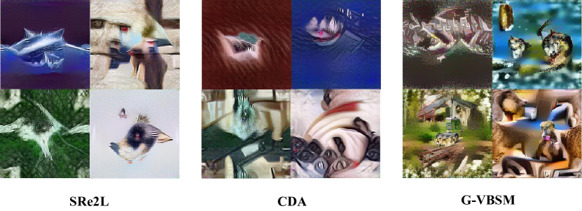
Figure 5: Visualization of the synthetic images of prior training-dependent dataset condensation methods.

Appendix G More Ablation Experiments

In this section, we present a series of ablation studies to further validate the design choices outlined in the main paper.

G.1 Backbone Choices of Data Synthesis on ImageNet-1k

Observer Model								Verified Model
ResNet-18	MobileNet-V2	EfficientNet-B0	ShuffleNet-V2	WRN-40-2	AlexNet	ConvNext-Tiny	DenseNet-121	ResNet-18	ResNet-50
✓	✓	✓	✓					38.7	42.0
✓	✓	✓	✓	✓				36.7	43.3
✓	✓	✓	✓		✓			39.0	43.8
✓	✓	✓	✓	✓	✓			37.4	43.1
✓	✓	✓	✓	✓	✓	✓	✓	34.8	40.6

Table 12: Ablation studies on ImageNet-1k with IPC 10. Verify the influence of backbone choices on data synthesis with $\mathbb{C}\mathbb{O}\mathbb{N}\mathbb{F}\mathbb{I}\mathbb{G}$ C ($\zeta=1.5$).

The results in Table 12 demonstrate the significant impact of backbone architecture selection on the performance of dataset distillation. This study employs the optimal configuration, which includes ResNet-18, MobileNet-V2, EfficientNet-B0, ShuffleNet-V2, and AlexNet.

G.2 Backbone Choices of Soft Label Generation on ImageNet-1k

Observer Model					Cost Time (s)	Verified Model
ResNet-18	MobileNet-V2	EfficientNet-B0	ShuffleNet-V2	AlexNet		ResNet-18	ResNet-50	ResNet-101
✓	✓	✓	✓		598	9.1	9.5	6.2
✓	✓		✓		519	9.4	8.4	6.5
✓	✓		✓	✓	542	12.8	13.3	8.4

Table 13: Ablation studies on ImageNet-1k with IPC 1. Verify the influence of backbone choice on soft label generation with $\mathbb{C}\mathbb{O}\mathbb{N}\mathbb{F}\mathbb{I}\mathbb{G}$ G ($\zeta=2$).

Our strategy better backbone choice, which focuses on utilizing lighter backbone combinations for soft label generation, significantly enhances the generalization capabilities of the condensed dataset. Empirical studies conducted with IPC 1, and the results detailed in Table 13, show that optimal performance is achieved by using ResNet-18, MobileNet-V2, EfficientNet-B0, ShuffleNet-V2, and AlexNet for data synthesis. For soft label generation, the combination of ResNet-18, MobileNet-V2, ShuffleNet-V2, and AlexNet demonstrates most effective.

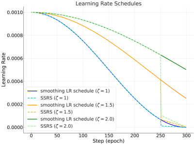
Figure 6: The visualization of SSRS and smoothing LR schedule.

G.3 Smoothing LR Schedule Analysis

Config	Slowdown Coefficient $\zeta$
	1.0	1.5	2.0	2.5	3.0
$\mathbb{C}\mathbb{O}\mathbb{N}\mathbb{F}\mathbb{I}\mathbb{G}$ C	24.5	28.2	30.6	32.4	31.8

Table 14: Ablation studies on ImageNet-1k with IPC 10. Additional experimental result of the slowdown coefficient $\zeta$ on the verified model MobileNet-V2.

Config	$\gamma$	Verified Model
		ResNet-18	ResNet-50	ResNet-101
$\mathbb{C}\mathbb{O}\mathbb{N}\mathbb{F}\mathbb{I}\mathbb{G}$ F	0.997	47.6	53.5	52.0
$\mathbb{C}\mathbb{O}\mathbb{N}\mathbb{F}\mathbb{I}\mathbb{G}$ F	0.9975	47.4	54.0	50.9
$\mathbb{C}\mathbb{O}\mathbb{N}\mathbb{F}\mathbb{I}\mathbb{G}$ F	0.99775	47.3	53.7	50.3
$\mathbb{C}\mathbb{O}\mathbb{N}\mathbb{F}\mathbb{I}\mathbb{G}$ F	0.997875	47.8	53.8	50.7

Table 15: Ablation studies on ImageNet-1k with IPC 10. Verify the effectiveness of ALRS in post-evaluation.

Due to space limitations in the main paper, the experimental results for MobileNet-V2, which are not included in Table 3 Left, are presented in Table 14. Additionally, we investigate Adaptive Learning Rate Scheduler (ALRS), an algorithm that adjusts the learning rate based on training loss. Although ALRS did not produce effective results, it provides valuable insights for future research. This scheduler was first introduced in [33] and is described as follows:

$$\mu(i)=\mu(i-1)\gamma^{\mathbbm{1}\left[\frac{|L_{i}-L_{i-1}|}{|L_{i}|}\leq h_{1}\text{ and }|L_{i}-L_{i-1}|\leq h_{2}\right]},$$

Here, $\gamma$ represents the decay rate, $L_{i}$ is the training loss at the $i$-th iteration, and $h_{1}$ and $h_{2}$ are the first and second thresholds, respectively, both set by default to 0.02. We list several values of $\gamma$ that demonstrate the best empirical performance in Table 15. These results allow us to conclude that our proposed smoothing LR schedule outperforms ALRS in the dataset condensation task.

Ultimately, we introduce a learning rate scheduler superior to the traditional smoothing LR schedule in scenarios with high IPC. This enhanced strategy, named early Smoothing-later Steep Learning Rate Schedule (SSRS), integrates the smoothing LR schedule with MultiStepLR. It intentionally implements a significant reduction in the learning rate during the final epochs of training to accelerate model convergence. The formal definition of SSRS is as follows:

$$\mu(i)=\begin{cases}\frac{1+\textrm{cos}(i\pi/\zeta N)}{2}&,i\leq\frac{5N}{6},\\ \vspace{2pt}\frac{1+\textrm{cos}(5\pi/\zeta 6)}{2}\frac{(6N-6i)}{6N}&,i>\frac{5N}{6}.\end{cases}\\$$ (33)

Config	Scheduler Type	Verified Model
		ResNet-18	ResNet-50	ResNet-101	MobileNet-V2
$\mathbb{C}\mathbb{O}\mathbb{N}\mathbb{F}\mathbb{I}\mathbb{G}$ G	smoothing LR schedule	56.4	62.2	62.3	54.7
$\mathbb{C}\mathbb{O}\mathbb{N}\mathbb{F}\mathbb{I}\mathbb{G}$ G	SSRS	57.4	63.0	63.6	56.5

Table 16: Ablation studies on ImageNet-1k with IPC 40. Verify the effectiveness of SSRS in post-evaluation.

Note that the visualization of SSRS can be found in Fig. 6. Meanwhile, the comparative experimental results of SSRS and the smoothing LR schedule are detailed in Table 16. Notably, SSRS enhances the verified model’s performance without incurring additional overhead.

G.4 Understanding of EMA-based Evaluation

$\mathbb{C}\mathbb{O}\mathbb{N}\mathbb{F}\mathbb{I}\mathbb{G}$ F	EMA Rate	0.99	0.999	0.9999	0.999945
	Accuracy	48.2	48.1	22.1	0.45

Table 17: Ablation studies on ImageNet-1k with IPC 10. Verify the effect of EMA Rate in EMA-based Evaluation.

The EMA Rate, a crucial hyperparameter governing the EMA update rate during post-evaluation, significantly influences the final results. Additional experimental outcomes, presented in Table 17, reveal that the EMA Rate 0.99 we adopt in the main paper yields optimal performance.

G.5 Ablation Studies on CIFAR-10

This section details the process of deriving hyperparameter configurations for CIFAR-10 through exploratory studies. The demonstrated superiority of our EDC method over traditional approaches, as detailed in our main paper, suggests that conventional dataset condensation techniques like MTT [14] and KIP [26] are not the sole options for achieving superior performance on small-scale datasets.

Iteration	25	50	75	100	125	1000
Accuracy	42.1	42.4	42.7	42.5	42.3	41.8

Table 18: Ablation studies on CIFAR-10 with IPC 10. We employ ResNet-18 exclusively for data synthesis and soft label generation, examining the impact of iteration count during post-evaluation and adhering to RDED’s consistent hyperparameter settings.

Data Synthesis		Soft Label Generation		Verified Model
w/ pre-train	w/o pre-train	w/ pre-train	w/o pre-train	ResNet-18	ResNet-50	ResNet-101	MobileNet-V2
✗	✓	✗	✓	77.7	73.0	68.2	38.2
✗	✓	✓	✗	60.5	56.3	52.2	39.9
✓	✗	✓	✗	60.0	56.1	50.7	39.0
✓	✗	✗	✓	74.9	70.9	61.4	38.2

Table 19: Ablation studies on CIFAR-10 with IPC 10. Hyperparameter settings follow those in Table 10, excluding the scheduler and batch size, which are set to smoothing LR schedule ($\zeta=2$) and 50, respectively.

EMA Rate	Batch Size	Verified Model
		ResNet-18	ResNet-50	ResNet-101	MobileNet-V2
0.99	50	77.7	73.0	68.2	38.2
0.999	50	13.1	11.8	11.6	11.2
0.9999	50	10.0	10.0	10.0	10.0
0.99	25	78.1	76.0	71.8	42.1
0.99	10	76.0	70.0	57.7	42.9

Table 20: Ablation studies on CIFAR-10 with IPC 10. Explore the influence of EMA Rate and batch size in post-evaluation. Hyperparameter settings follow those in Table 10, excluding the scheduler, which are set to smoothing LR schedule ($\zeta=2$).

Scheduler	Option	Verified Model
		ResNet-18	ResNet-50	ResNet-101	MobileNet-V2
Smoothing LR Schedule	$\zeta=2$	78.1	76.0	71.8	42.4
Smoothing LR Schedule	$\zeta=3$	77.3	75.0	68.5	41.1
MultiStepLR	$\gamma=0.5$, milestones=[800,900,950]	79.1	76.0	67.1	42.0
MultiStepLR	$\gamma=0.25$, milestones=[800,900,950]	77.7	75.8	67.0	40.3

Table 21: Ablation studies on CIFAR-10 with IPC 10. Explore the influence of various scheduler in post-evaluation. Hyperparameter settings follow those in Table 10.

Our quantitative experiments, detailed in Table 18, pinpoint 75 iterations as the empirically optimal count. This finding highlights that, for smaller datasets with limited samples and fewer categories, fewer iterations are required to achieve superior results.

Subsequently, we evaluate the effectiveness of using a pre-trained model on ImageNet-1k for dataset condensation on CIFAR-10. Our study differentiates two training pipelines: the first involves 100 epochs of pre-training followed by 10 epochs of fine-tuning (denoted as ‘w/ pre-train’), and the second comprises training from scratch for 10 epochs (denoted as ‘w/o pre-train’). The results, presented in Table 19, indicate that pre-training on ImageNet-1k does not significantly enhance dataset distillation performance.

We further explore how batch size and EMA Rate affect the generalization abilities of the condensed dataset. Results in Table 20 show that a reduced batch size of 25 enhances performance on CIFAR-10.

In our final set of experiments, we compare MultiStepLR and smoothing LR schedules. As detailed in Table 21, MultiStepLR is superior for ResNet-18 and ResNet-50, whereas the smoothing LR schedule is more effective for ResNet-101 and MobileNet-V2.

Appendix H Synthesized Image Visualization

The visualization of the condensed dataset is showcased across Figs. 7 to 11. Specifically, Figs. 7, 9, 10, and 11 present the datasets synthesized from ImageNet-1k, Tiny-ImageNet, CIFAR-100, and CIFAR-10, respectively.

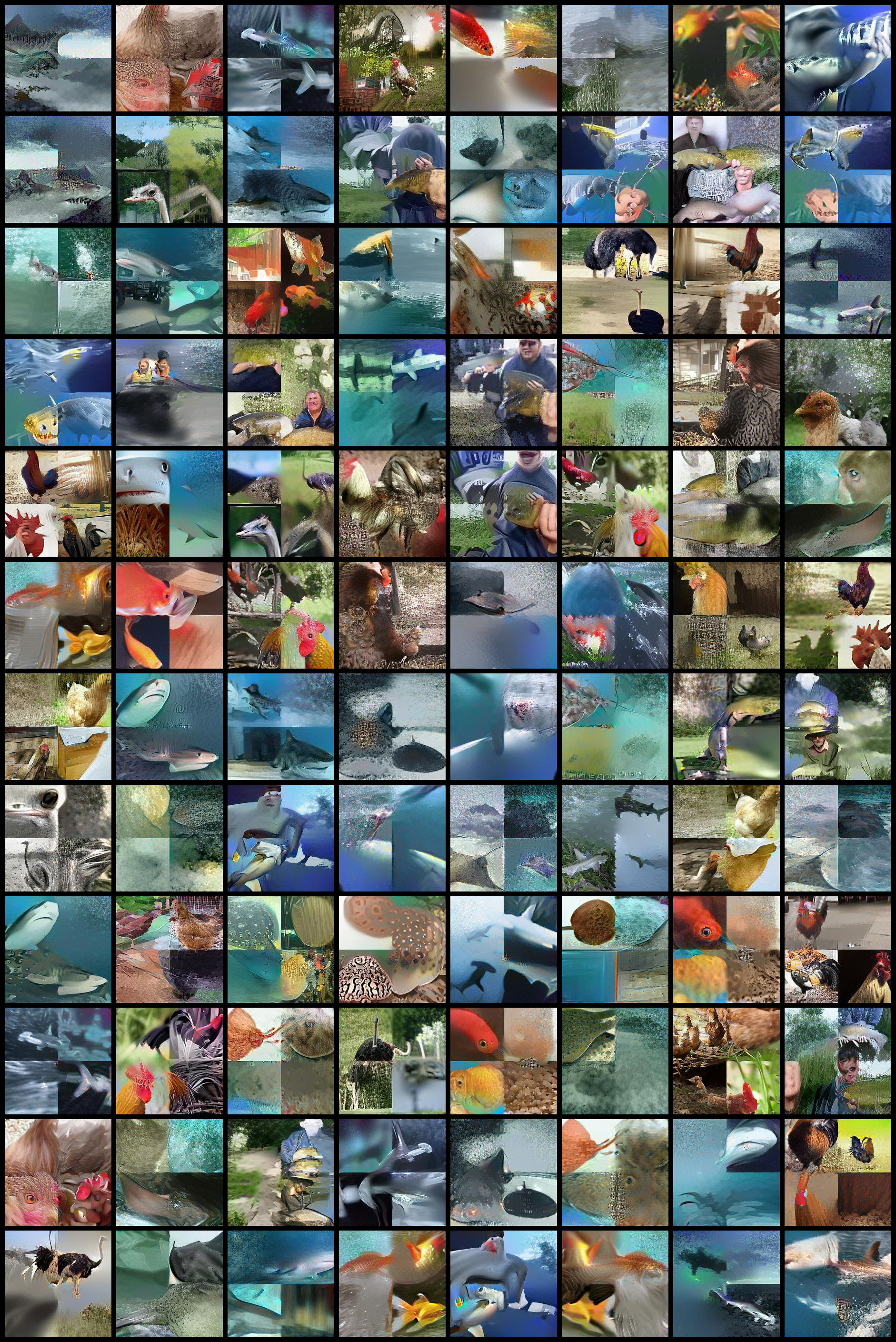
Figure 7: Synthetic data visualization on ImageNet-1k randomly selected from EDC.

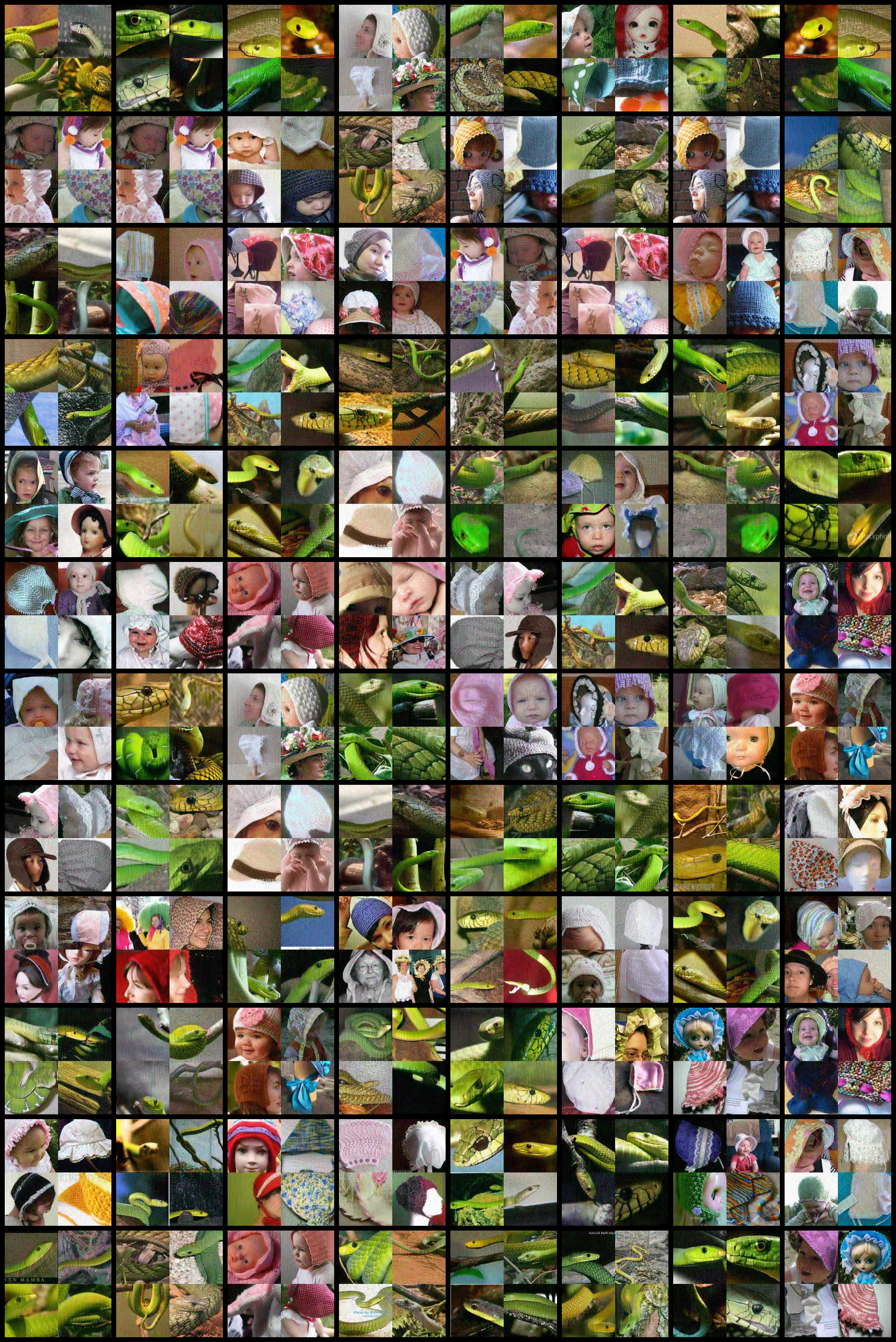
Figure 8: Synthetic data visualization on ImageNet-10 randomly selected from EDC.

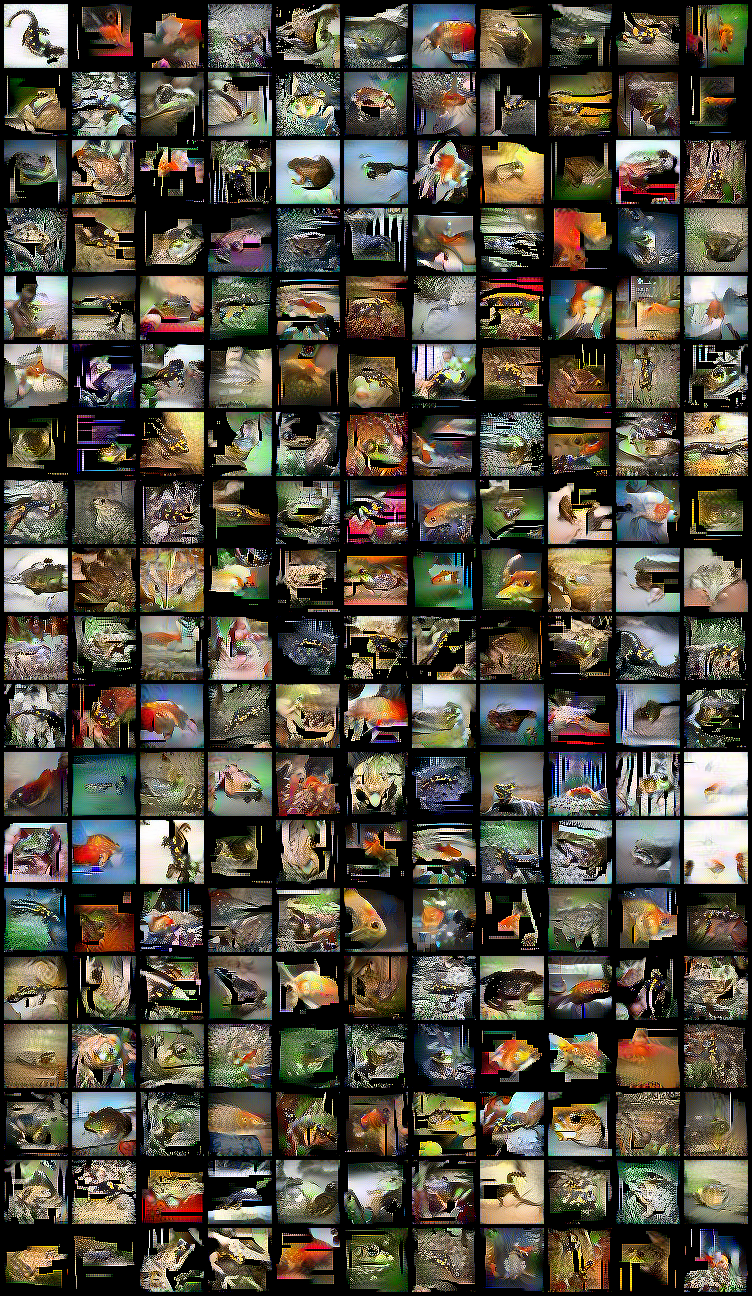
Figure 9: Synthetic data visualization on Tiny-ImageNet randomly selected from EDC.

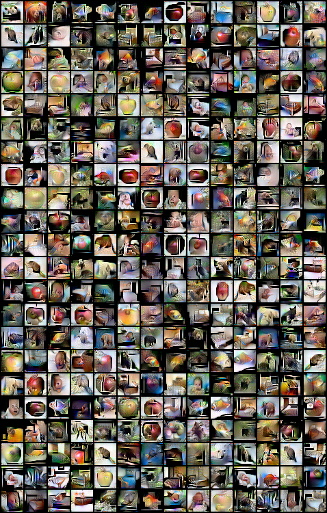
Figure 10: Synthetic data visualization on CIFAR-100 randomly selected from EDC.

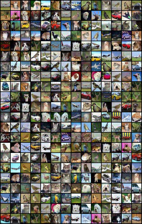
Figure 11: Synthetic data visualization on CIFAR-10 randomly selected from EDC.

References

- He et al. [2016a] K. He, X. Zhang, and S. Ren, “Deep residual learning for image recognition,” in Computer Vision and Pattern Recognition. Las Vegas, NV, USA: IEEE, Jun. 2016, pp. 770–778.
- He et al. [2016b] K. He, X. Zhang, S. Ren, and J. Sun, “Identity mappings in deep residual networks,” in European Conference on Computer Vision. Amsterdam, North Holland, The Netherlands: Springer, Oct. 2016, pp. 630–645.
- Brown et al. [2020] T. Brown, B. Mann, N. Ryder, M. Subbiah, J. D. Kaplan, P. Dhariwal, A. Neelakantan, P. Shyam, G. Sastry, A. Askell et al., “Language models are few-shot learners,” Advances in neural information processing systems, vol. 33, pp. 1877–1901, 2020.
- Dosovitskiy et al. [2020] A. Dosovitskiy, L. Beyer, A. Kolesnikov, D. Weissenborn, X. Zhai, T. Unterthiner, M. Dehghani, M. Minderer, G. Heigold, S. Gelly et al., “An image is worth 16x16 words: Transformers for image recognition at scale,” in International Conference on Learning Representations. Event Virtual: OpenReview.net, May 2020.
- Wang et al. [2020] H. Wang, S. Lohit, M. Jones, and Y. Fu, “Knowledge distillation thrives on data augmentation,” arXiv preprint arXiv:2012.02909, 2020.
- Shao et al. [2024] S. Shao, Z. Shen, L. Gong, H. Chen, and X. Dai, “Precise knowledge transfer via flow matching,” arXiv preprint arXiv:2402.02012, 2024.
- Masarczyk and Tautkute [2020] W. Masarczyk and I. Tautkute, “Reducing catastrophic forgetting with learning on synthetic data,” in Computer Vision and Pattern Recognition Workshops. Virtual Event: IEEE, Jun. 2020, pp. 252–253.
- Sangermano et al. [2022] M. Sangermano, A. Carta, A. Cossu, and D. Bacciu, “Sample condensation in online continual learning,” in International Joint Conference on Neural Networks. Padua, Italy: IEEE, Jul. 2022, pp. 1–8.
- Zhao and Bilen [2021] B. Zhao and H. Bilen, “Dataset condensation with differentiable siamese augmentation,” in International Conference on Machine Learning, M. Meila and T. Zhang, Eds., vol. 139. Virtual Event: PMLR, 2021, pp. 12 674–12 685.
- Such et al. [2020] F. P. Such, A. Rawal, J. Lehman, K. O. Stanley, and J. Clune, “Generative teaching networks: Accelerating neural architecture search by learning to generate synthetic training data,” in International Conference on Machine Learning, vol. 119. Virtual Event: PMLR, Jul. 2020, pp. 9206–9216.
- Zhao and Bilen [2023] B. Zhao and H. Bilen, “Dataset condensation with distribution matching,” in Winter Conference on Applications of Computer Vision. Waikoloa, Hawaii: IEEE, Jan. 2023, pp. 6514–6523.
- Zhao et al. [2021] B. Zhao, K. R. Mopuri, and H. Bilen, “Dataset condensation with gradient matching,” in International Conference on Learning Representations. Virtual Event: OpenReview.net, May 2021.
- Liu et al. [2017] Z. Liu, J. Li, Z. Shen, G. Huang, S. Yan, and C. Zhang, “Learning efficient convolutional networks through network slimming,” in International Conference on Computer Vision. IEEE, 2017, pp. 2736–2744.
- Cazenavette et al. [2022] G. Cazenavette, T. Wang, A. Torralba, A. A. Efros, and J. Zhu, “Dataset distillation by matching training trajectories,” in Computer Vision and Pattern Recognition. New Orleans, LA, USA: IEEE, Jun. 2022.
- Sajedi et al. [2023] A. Sajedi, S. Khaki, E. Amjadian, L. Z. Liu, Y. A. Lawryshyn, and K. N. Plataniotis, “Datadam: Efficient dataset distillation with attention matching,” in International Conference on Computer Vision. Paris, France: IEEE, Oct. 2023, pp. 17 097–17 107.
- Liu et al. [2023a] Y. Liu, J. Gu, K. Wang, Z. Zhu, W. Jiang, and Y. You, “DREAM: efficient dataset distillation by representative matching,” arXiv preprint arXiv:2302.14416, 2023.
- Russakovsky et al. [2015] O. Russakovsky, J. Deng, H. Su, J. Krause, S. Satheesh, S. Ma, Z. Huang, A. Karpathy, A. Khosla, M. Bernstein et al., “Imagenet large scale visual recognition challenge,” International Journal of Computer Vision, vol. 115, no. 3, pp. 211–252, 2015.
- Yin et al. [2023] Z. Yin, E. P. Xing, and Z. Shen, “Squeeze, recover and relabel: Dataset condensation at imagenet scale from A new perspective,” in Neural Information Processing Systems. NIPS, 2023.
- Yin and Shen [2024] Z. Yin and Z. Shen, “Dataset distillation in large data era,” 2024. [Online]. Available: https://openreview.net/forum?id=kpEz4Bxs6e
- Shao et al. [2023] S. Shao, Z. Yin, X. Zhang, and Z. Shen, “Generalized large-scale data condensation via various backbone and statistical matching,” arXiv preprint arXiv:2311.17950, 2023.
- Krizhevsky et al. [2009] A. Krizhevsky, G. Hinton et al., “Learning multiple layers of features from tiny images,” 2009.
- Sun et al. [2023] P. Sun, B. Shi, D. Yu, and T. Lin, “On the diversity and realism of distilled dataset: An efficient dataset distillation paradigm,” arXiv preprint arXiv:2312.03526, 2023.
- Wang et al. [2018] T. Wang, J.-Y. Zhu, A. Torralba, and A. A. Efros, “Dataset distillation,” arXiv preprint arXiv:1811.10959, 2018.
- Cui et al. [2023] J. Cui, R. Wang, S. Si, and C. Hsieh, “Scaling up dataset distillation to imagenet-1k with constant memory,” in International Conference on Machine Learning, vol. 202. Honolulu, Hawaii, USA: PMLR, 2023, pp. 6565–6590.
- Wang et al. [2022] K. Wang, B. Zhao, X. Peng, Z. Zhu, S. Yang, S. Wang, G. Huang, H. Bilen, X. Wang, and Y. You, “Cafe: Learning to condense dataset by aligning features,” in Computer Vision and Pattern Recognition. New Orleans, LA, USA: IEEE, Jun. 2022, pp. 12 196–12 205.
- Nguyen et al. [2020] T. Nguyen, Z. Chen, and J. Lee, “Dataset meta-learning from kernel ridge-regression,” arXiv preprint arXiv:2011.00050, 2020.
- Kim et al. [2022] J. Kim, J. Kim, S. J. Oh, S. Yun, H. Song, J. Jeong, J. Ha, and H. O. Song, “Dataset condensation via efficient synthetic-data parameterization,” in International Conference on Machine Learning, vol. 162. Baltimore, Maryland, USA: PMLR, Jul. 2022, pp. 11 102–11 118.
- Zhou et al. [2023] D. Zhou, K. Wang, J. Gu, X. Peng, D. Lian, Y. Zhang, Y. You, and J. Feng, “Dataset quantization,” in Proceedings of the IEEE/CVF International Conference on Computer Vision, 2023, pp. 17 205–17 216.
- Hinton et al. [2015] G. Hinton, O. Vinyals, and J. Dean, “Distilling the knowledge in a neural network,” 2015. [Online]. Available: https://arxiv.org/abs/1503.02531
- Gou et al. [2021] J. Gou, B. Yu, S. J. Maybank, and D. Tao, “Knowledge distillation: A survey,” International Journal of Computer Vision, vol. 129, no. 6, pp. 1789–1819, 2021.
- Chen et al. [2024] H. Chen, Y. Zhang, Y. Dong, and J. Zhu, “Rethinking model ensemble in transfer-based adversarial attacks,” in International Conference on Learning Representations. Vienna, Austria: OpenReview.net, May 2024.
- Foret et al. [2020] P. Foret, A. Kleiner, H. Mobahi, and B. Neyshabur, “Sharpness-aware minimization for efficiently improving generalization,” in International Conference on Learning Representations, 2020.
- Chen et al. [2022] H. Chen, S. Shao, Z. Wang, Z. Shang, J. Chen, X. Ji, and X. Wu, “Bootstrap generalization ability from loss landscape perspective,” in European Conference on Computer Vision. Springer, 2022, pp. 500–517.
- Liu et al. [2023b] H. Liu, T. Xing, L. Li, V. Dalal, J. He, and H. Wang, “Dataset distillation via the wasserstein metric,” arXiv preprint arXiv:2311.18531, 2023.
- Du et al. [2022] J. Du, D. Zhou, J. Feng, V. Tan, and J. T. Zhou, “Sharpness-aware training for free,” in Advances in Neural Information Processing Systems, vol. 35. New Orleans, Louisiana, USA: NIPS, Dec. 2022, pp. 23 439–23 451.
- Bahri et al. [2021] D. Bahri, H. Mobahi, and Y. Tay, “Sharpness-aware minimization improves language model generalization,” arXiv preprint arXiv:2110.08529, 2021.
- Tavanaei [2020] A. Tavanaei, “Embedded encoder-decoder in convolutional networks towards explainable AI,” vol. abs/2007.06712, 2020. [Online]. Available: https://arxiv.org/abs/2007.06712
- Sandler et al. [2018] M. Sandler, A. G. Howard, M. Zhu, A. Zhmoginov, and L. Chen, “Mobilenetv2: Inverted residuals and linear bottlenecks,” in Computer Vision and Pattern Recognition. Salt Lake City, UT, USA: IEEE, Jun. 2018, pp. 4510–4520.
- Touvron et al. [2021] H. Touvron, M. Cord, M. Douze, F. Massa, A. Sablayrolles, and H. Jégou, “Training data-efficient image transformers & distillation through attention,” in International Conference on Machine Learning, M. Meila and T. Zhang, Eds., vol. 139. Virtual Event: PMLR, Jul. 2021, pp. 10 347–10 357.
- Liu et al. [2021] Z. Liu, Y. Lin, Y. Cao, H. Hu, Y. Wei, Z. Zhang, S. Lin, and B. Guo, “Swin transformer: Hierarchical vision transformer using shifted windows,” in International Conference on Computer Vision, 2021, pp. 10 012–10 022.
- Tan and Le [2019] M. Tan and Q. Le, “Efficientnet: Rethinking model scaling for convolutional neural networks,” in International conference on machine learning. PMLR, 2019, pp. 6105–6114.
- Liu et al. [2022] Z. Liu, H. Mao, C.-Y. Wu, C. Feichtenhofer, T. Darrell, and S. Xie, “A convnet for the 2020s,” in Proceedings of the IEEE/CVF Conference on Computer Vision and Pattern Recognition, 2022, pp. 11 976–11 986.
- Zhang et al. [2018] X. Zhang, X. Zhou, M. Lin, and J. Sun, “Shufflenet: An extremely efficient convolutional neural network for mobile devices,” in Computer Vision and Pattern Recognition, 2018, pp. 6848–6856.
- Srinivas and Babu [2015] S. Srinivas and R. V. Babu, “Data-free parameter pruning for deep neural networks,” arXiv preprint arXiv:1507.06149, 2015.
- Prabhu et al. [2020] A. Prabhu, P. H. S. Torr, and P. K. Dokania, “Gdumb: A simple approach that questions our progress in continual learning,” in European Conference on Computer Vision. Springer, Jan 2020, p. 524–540.
- Paszke et al. [2019] A. Paszke, S. Gross, F. Massa, A. Lerer, J. Bradbury, G. Chanan, T. Killeen, Z. Lin, N. Gimelshein, L. Antiga et al., “Pytorch: An imperative style, high-performance deep learning library,” in Neural Information Processing Systems, Vancouver, BC, Canada, Dec. 2019.
- Zhou et al. [2024] M. Zhou, Z. Yin, S. Shao, and Z. Shen, “Self-supervised dataset distillation: A good compression is all you need,” arXiv preprint arXiv:2404.07976, 2024.