Controlling quantum vortex dynamics and vortex-antivortex annihilation in Bose-Einstein condensates with optical lattices

Abstract

Superfluids with strong spatial modulation can be experimentally produced in the area of cold atoms under the influence of optical lattices. Here we address ⁸⁷Rb bosons at T=0 K in a flat geometry under the influence of a periodic potential with the Gross-Pitaevskii theory. The statics and dynamics of vortex excitations are studied in the case of one dimensional (1D) and of two dimensional (2D) optical lattices, as function of the intensity of the optical lattice. We compute how the vortex energy depends on the position of its core and the energy barrier that a vortex has to surmount in order to move in the superfluid. The dynamics of a vortex dipole, a pair of vortices of opposite chirality, differ profoundly from the case of a uniform superfluid. In the 1D case, when parallel ridges of density are present, the dynamics depends on the positions of the two vortices. If they are in the same channel between two ridges, then the two vortices approach each other until they annihilate each other in a short time. If the two vortices are in distinct channels the dipole undergoes a rigid translation but with a velocity depending on the intensity of the optical lattice and this translation velocity can even change sign with respect to the case of the uniform superfluid. Superimposed on this translation an oscillatory motion is also present. A superposition of translation along a channel and an oscillation is also found with a single vortex when the system is bounded inside a circular trap. These oscillatory motions can be both longitudinal, i.e. along the channel, as well as transverse. In all cases the transverse motions are one-side, in the sense that the vortex core never crosses the equilibrium position nearest the starting position. In the case of the 2D lattices we study (square, triangular and honeycomb), the two vortices of a dipole move mainly by jumps between equilibrium positions and approach each other until annihilation. This behavior has some similarity with what has been found for a vortex dipole in the supersolid state of dipolar bosons. We show that a rapid rump-down of the optical potential improves the visibility of the density holes at the vortex core.

I Introduction and summary

One of the key properties of a superfluid is the presence of quantized vorticity. In the case of bosons this has been experimentally verified in superfluid ⁴He donnelly and in Bose-Einstein condensates (BEC) of cold atoms fetter . A quantum vortex is an excitation of the system with quantized circulation and angular momentum and usually such excitation is studied in a superfluid that is uniform or with an inhomogeneity that is weak on the scale of the healing length of the superfluid. At present there is the possibility of studying vortices in spatially strongly inhomogeneous systems, both in terms of the spatial scale as well as in terms of large contrast between the maximum and the minimum densities. In the realm of cold atoms it is possible to generate a periodic potential (optical lattice, OL) acting on the atoms and this potential is obtained by standing waves of suitable crossing light beamsolattice . The period of the optical lattice can be comparable to the healing length and the local density can vary even by orders of magnitude. A recent experiment tao has verified the theoretical prediction leg70 that even at the lowest temperatures the superfluid fraction of the superfluid is less than unity due to the induced density modulation.

Another system that is predicted to be a spatially strongly inhomogeneous superfluid is a submonolayer of ⁴He adsorbed on a substrate of fluorographene, a sheet of graphene decorated by fluorine atoms. The adsorption potential of a He atom on this substrate is strongly corrugated but not so much to cause localization of the atoms like on graphite. Theory moroni shows that the system is superfluid and the local density has a very large excursion in space. A supersolid (SS) offers another example of a strongly inhomogeneous superfluid. In a SS the inhomogeneity arises from a spontaneous broken symmetry of the translational invariance. Such SS state has been found in cold atom systems, for instance in dipolar bosons like ¹⁶⁴Dy lchomaz . Again the local density can vary by a large amount and the healing length is comparable with the lattice parameter of the SS.

Different ways have been devised to create vortices in BEC superfluids, such as phase imprintingisoshima , by dragging obstacles neely , by means of artificial gauge fieldsjlin , and more recently using a versatile, deterministic 2D vortex collider in homogeneous atomic superfluidskwon .

Complex dynamics of vortices under the action of the optical lattice in a trapped BEC sample have been unveiled in a theoretical study of vortices within the two-dimensional GP equation with the OL and magnetic trapkevrek , where it was found that depending on the phase of the OL relative to the parabolic magnetic trap, it is possible either to trap the vortex at the center of the trap, or the vortex moves along an unwinding spiral, towards the periphery of the trap.

The interplay of lattice physics and rotation physics was studied by calculating the vortex-lattice structures near a Mott transitiongoldbaum . A single BEC loaded in a rotating OL can show a rich variety of vortex structural transitionshpu

There have been predictions of novel types of vortex states of repulsive BECs confined by a shallow optical lattice (matter-wave gap vortices), which are spatially localized and dynamically stable in 2D as well as in 3D optical latticeskivshar .

Interestingly, vortex dynamics in non-homogeneous systems can be linked to ”glitches” in rotating pulsars, i.e. a sudden speed up of the spinning stars, occurring at random intervals. These events are believed to be a manifestation of the presence of a superfluid component in the stellar interior, the glitch occurring when many vortices jump from the inside of the star to the solid crust, transferring angular momentum and thus speeding it up. It has been shown recently, using cold atom experiments as analogs of neutron stars, that this requires simultaneous crystalline and superfluid phases, i.e. a supersolid state epoli .

A subject that apparently has received very little attention is the behavior of vortex dipoles. Such configurations have been experimentally obtained in BEC in the work of Refs.neely . However topics such as the interaction of such dipoles and the ensuing dynamics are still unexplored. Our study provide an insight into these issues, and how they are modified by optical lattice.

All this gives a motivation for studying vortices in strongly inhomogeneous superfluids, the aim of the present paper. We show how strongly the dynamics of vortices and the lifetimes of pairs of vortex-antivortex are affected by an optical potential. The experimental realization of generation of vortex dipoles in a suitable trap for cold atoms kwon open the possibility of experimental verification of our predictions.

Vortices in the SS state of matter in dipolar bosons have been theoretically addressed gallemi ; casotti ; gallemi1 ; Anc21 in recent years and some relevant phenomena have been uncovered, like a reduced angular momentum associated to the quantum of circulation gallemi . A peculiar behavior has been found Anc21 in the dynamic of a vortex dipole, i.e. a pair of vortices of opposite chirality, in a SS. In a uniform superfluid, when the distance $l$ between the two vortices is larger than the healing length $\xi$, the pair is a stable entity and moves with a constant velocity as a rigid body in a direction perpendicular to the vector $\vec{l}$ joining the two vortices. Contrary to this, in dipolar bosons in a SS state it was found that the two vortices moves by jumps between equilibrium sites in the lattice and approach each other until the two vortices annihilate themselves in a short time. At the basis of this behavior is a basic property of a vortex in a SS: it is energetically favorable to have its core at a discrete set of positions, the locus of minimum density. The natural question is if such properties are specific of a SS state or if they are generic ones when a density modulation is present, whatever is its origin. To answer this question we address in the present paper the study of bosons in an external periodic potential like that produced by light standing waves. We study the ground state and vortices of the standard model of BEC, point-like bosons with a contact interaction, in the case of ⁸⁷Rb with the Gross-Pitaevskii equation in an external periodic potential $V_{ext}(\vec{r})$. We consider the case of modulation in one dimension (1D) and in two dimensions (2D) for three lattices: square, triangular and honeycomb.

The system is subject to periodic boundary conditions in all three space directions, and translational invariance along the z-direction perpendicular to the lattice potential plane is assumed. The length in the z direction is of order of the healing length of the superfluid so that the system can be considered as a quasi-two dimensional system.

In the studied range of intensity of our optical potentials we find that the bosons are in a superfluid state with a reduced superfluid fraction. The local density is a periodic function of position reflecting the symmetry of the optical potential and the excursion between maxima and minima can be very large, depending on the strength of the modulation of $V_{ext}(\vec{r})$. In a uniform superfluid the vortex excitation energy $\Delta E_{v}$ does not depend on the position of its core. On the contrary, in the presence of the optical potential $\Delta E_{v}$ depends on the position of its core and it is a strong function of the local density. The minima of $\Delta E_{v}$ are at the positions of the minima of the local density, i.e. at the maxima of $V_{ext}(\vec{r})$, consistently with the observation of pinning of the vortex at the low density site of an OL was observedduine . Therefore $\Delta E_{v}$ is a periodic function of position and this has a dramatic effect on the dynamics of vortices. The flow field of a vortex is strongly deformed from the circular shape of the uniform case and we characterize the vortex excitation energy and its structure as function of the amplitude of the optical potential.

The dynamics of a vortex dipole is also strongly affected by the presence of the optical potential.

For a 2D potential, where the equilibrium positions of the vortex are isolated points, the dipole moves mainly by jumps between equilibrium sites approaching each other until the two vortices annihilate themself in a short time. In our theory no thermal or stochastic effects are present and these jumps are manifestations of tunneling of the vortices between equilibrium sites.

The behavior is different in the case of a 1D modulation where the equilibrium positions for a vortex form a series of parallel lines in the x-y plane.

If the two vortices of the dipole are located in the same channel they do not translate but they move one against the other until they annihilate and the excitation energy goes into phonons of the superfluid. If the two vortices are located in adjacent channels they move along these channels and the motion is a composition of a uniform translation and of an oscillation. In all cases the translation velocity of the pair differs from that expected for a uniform superfluid and it can even invert the direction of motion for large amplitude of the optical potential. A combination of translation and oscillation is found also for a single vortex in a trap in presence of a 1D OL.. The frequency of this oscillation is the same as in the case of a vortex dipole moving along two neighboring channels. Therefore this oscillatory motion seems to be an intrinsic and novel character of the motion of a vortex moving along a channel. Notice that this oscillatory motion is quite different from that of a massive particle around a minimum energy position because the vortex oscillation is one-side, i.e. the vortex never crosses the position of the minimum energy and it remains on the side from which it started.

The local density goes to zero at the position of the vortex core. In the case of a strong modulation experimentally it can be difficult to detect the presence of a vortex because there is a small contrast between the vanishing density of the vortex core and the small value of the density at the minima of the modulated system. We show that by starting from a state with a number of vortices in the modulated superfluid, such vortices remain in the homogeneous superfluid after that the optical potential is suddenly removed, allowing for an easier visual detection due to the increased contrast between the vanishing density at the core positions and the density of the surrounding, almost homogeneous phase.

The content of the paper is as follow. In Sect.II the theory and the computational method are described. In Sect. III the ground state, the vortex state and the dynamics of a vortex pair are studied in the case of 1D optical potential. In this Section we study also the dynamics of a vortex when the system in confined in a circular trap in the x-y plane. The case of 2D optical potentials is studied similarly in Sect. IV. In Sect. V we study the time evolution of a confined system after the optical potential is removed, as a way to directly image vortex positions in these highly inhomogeneous systems. Our conclusions are contained in Sect. VI.

II Method

The Gross-Pitaevskii (GP) energy functional for the Bose system reads

$$E=\int d{\bf r}\,\left[{\hbar^{2}\over 2m}|\nabla\psi({\bf r})|^{2}+V({\bf r})\rho({\bf r})\right]\,+\frac{1}{2}g\int d{\bf r}\,\rho^{2}({\bf r})\,$$ (1)

where $V({\bf r})$ and $\rho({\bf r})=|\psi({\bf r})|^{2}$ represent the external potential and the boson number density, respectively. The coupling constant is $g=4\pi a_{s}\hbar^{2}/m$, $m$ being the atomic mass. The number density $\rho$ is normalized such that $\int_{V}\rho({\bf r})\,{\rm d}{\bf r}=N$ where $N$ is the total number of atoms. As model system we take ⁸⁷Rb atoms and the scattering length $a_{s}$ describing the (repulsive) Rb-Rb interaction is $a_{s}=100.4\,a_{0}$ marte .

Minimization of the action associated to Eq. (1) leads to the following Euler-Lagrange equation (GP equations)

$$i\hbar{\partial\psi(\vec{r},t)\over\partial t}=\left[-{\hbar^{2}\over 2m}\nabla^{2}+V(\vec{r})+g\rho(\vec{r},t)\right]\psi(\vec{r},t)\equiv H\psi(\vec{r},t)\,,$$ (2)

When steady states are studied the left hand side of Eq.(2) is replaced by $\mu\psi(\vec{r},t)$ where $\mu$ is the chemical potential. The numerical solutions of Eqs. (2) provide the time-evolution of the ⁸⁷Rb system with arbitrary $N$ in three-dimensions. The same equation in imaginary time allows us to obtain stationary state solutions starting from a suitable initial function. $\mu$ is determined so that the desired value of $N$ is achieved. We consider an external potential depending only in $x$ and $y$.

In our computations the length $L_{z}$ of the computation box is much smaller of the other sides. Under this condition we simplify the computation by neglecting the dependence of $\psi$ on the $z$ coordinate and therefore the calculations become effectively 2-dimensional. Accordingly, vortex states considered here are not subject to three-dimensional instabilities like corrugation/bending of the vortex core as the transverse dimension is effectively suppressed. For this reason often in the following we will describe the properties of the system as it appears in the x-y plane only.

Eq.(2) is solved either in real time or imaginary time by using Hamming’s predictor-modifier-corrector method initiated by a fourth-order Runge-Kutta-Gill algorithm Ral60 . The spatial mesh spacing and time step are chosen such that, during the real time evolution, excellent conservation of the total energy of the system is guaranteed.

We will use in the present work different forms for the external potential $V$ appearing in the GP equation (2). In particular, we will consider periodic potentials both in one dimension and in two dimensions, as described in the following Sections. These potentials are easily produced in experiments using crossed laser fields with appropriate wavelengths (optical lattices, OL).

III ⁸⁷Rb in 1D optical lattice

One-dimensional lattice potentials are often used in experiments. In the simplest form, like the one used here, they produce modulated density patterns characterized by a periodic alternation of stripes of maxima and minima in the gas density. Here we consider the form

$$V_{OL}(x)=2V_{0}\,cos^{2}(kx)$$ (3)

The wavevector $k$ determines the lattice constant of the periodic potential, $d=2\pi/k$. For the cases investigated here we chose $d=60000\,a_{0}=3.175\,\mu m$. The sizes of the supercell in the x-y plane are, for most of the calculations done, $L_{x}=L_{y}=44.45\,\mu m$, corresponding to $14$ stripes in the x direction, although for the sake of visibility the plots shown in this paper are often limited to smaller portions of the supercell.

Along the z-direction we chose the value $L_{z}=1.429\,\mu m$. The total number of atoms $N$ in most of our calculations is chosen so that it corresponds to an areal density $n_{a}=N/(L_{x}L_{y})=9.92\,\mu m^{-2}$. In the following, some calculations will be performed using larger supercell sizes $L_{x},L_{y}$, corresponding to $20$ stripes in the x direction. However, we will always take the number of atoms $N$ such that the areal density $n_{a}=N/(L_{x}L_{y})$ is not changed.

The healing length for the uniform system ($V_{0}=0$) is $\xi=\hbar/\sqrt{2m\mu}=1.039\,\mu m$, where $\mu=g\rho$ is the Rb chemical potential in the absence of the lattice modulation. Notice that $L_{z}$ is of the same order of magnitude of the healing length, and therefore our system can be considered quasi-2D. Due to the imposed translational invariance along the $z$ direction, along which the density is therefore constant, the calculations are effectively 2-dimensional, involving a spatial discrete mesh only in the x-y plane.

We will consider different values for the potential strength $V_{0}$ in the following, and often the following values $V_{0}=2,4,7,9\times 10^{-14}\,Ha$ have been used.

It is customary to express the lattice well depths $V_{0}$ in terms of the so-called recoil energy as $V_{0}=sE_{R}$, where

$$E_{R}=\frac{\hbar^{2}\pi^{2}}{2md^{2}}$$ (4)

In the present case $E_{R}=8.600\times 10^{-15}\,$ Ha. The values of $V_{0}$ quoted above therefore correspond to $s=2.3,4.6,8.1,10.5$. For much larger values of $s$ the bosons are expected to become localized forming rows of independent quasi-one dimensional superfluids.

In the following we will use a more manageable notation where the optical potential strength $V_{0}$ is expressed in terms of an adimensional quantity $\tilde{V}$ such that $V_{0}=\tilde{V}\times 10^{-14}$ Ha $=\tilde{V}\times 3.158\,nK$.

In Fig.1 we show for some values of $\tilde{V}$ the density along the x-axis, the direction of the modulation showing the periodic alternation of minima and maxima in the density profile. The values of the density at these extrema are reported in Table I, together with the calculated chemical potentials.

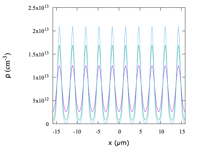
Figure 1: Density profiles (in units of $cm{-3}$) along the x-axis, for different values of $\tilde{V}$. From the highest to the lowest peak values: $\tilde{V}=(7,4,2)$.

It can be noticed that already an intensity $\tilde{V}=4$ the maximum density is ten times larger of the minimum density. Despite such large inhomogeneity the system is superfluid. The superfluid fraction can be computed from the non-classical translational inertia sep_joss_rica as

$$f_{s}=1-\lim_{v_{x}\to 0}\frac{\langle\hat{P}_{x}\rangle}{Nmv_{x}}$$ (5)

where $\langle\hat{P}_{x}\rangle=-i\hbar\int\psi^{\ast}(\vec{r})\partial\psi(\vec{r})/\partial xd\vec{r}$ is the expectation value of the momentum in the x-direction of the ⁸⁷Rb and $Nmv_{x}$ is the total momentum of the system if all the atoms were moving with the constant velocity $v_{x}$.

Alternatively, one could estimate the superfluid fraction from leg70

$$f_{s}=\frac{L_{x}^{2}}{\int_{0}^{L_{x}}dx<n(x)>\int_{0}^{L_{x}}dx<n(x)>^{-1}}$$ (6)

where $<n(x)>$ is the number density of the ground-state configuration averaged over the transverse y-z directions. We find that the values of $f_{s}$ from the two definitions agree with each other to within $1\%$.

The dependence on $\tilde{V}$ of the superfluid fraction (in the direction parallel to the modulation) is shown in Fig.(2) and the values of $f_{s}$ for some values of $\tilde{V}$ are given in Table I. We notice that the suppression of the superfluid fraction in the direction of the modulation is quite substantial. In the direction perpendicular to the modulation, i.e. in the y direction, the superfluid fraction is unity in all cases. Therefore we have a strongly anisotropic superfluid.

Figure 2: Superfluid fraction in the 1D lattice as a function of $\tilde{V}$ in the direction of the modulation.

	$\tilde{V}$	$\rho_{min}$ $(cm^{-3})$	$\rho_{max}$ $(cm^{-3})$	$\mu$ ($nK$)	$f_{s}$
	$0$	$6.943\times 10^{12}$	$6.943\times 10^{12}$	$2.584$	$1$
	$2$	$2.609\times 10^{12}$	$1.256\times 10^{13}$	$8.062$	$0.744$
	$4$	$0.777\times 10^{12}$	$1.696\times 10^{13}$	$11.923$	$0.355$
	$7$	$0.136\times 10^{12}$	$2.098\times 10^{13}$	$15.839$	$0.095$

Table 1: $\tilde{V}$ is the amplitude of the periodic potential; $\rho_{min}$ and $\rho_{max}$ are the density values at the bottom and top of the modulated density; $\mu$ is the chemical potential and $f_{s}$ is the superfluid fraction in the x-direction computed from the non-classical translational inertia.

III.1 Single vortex properties

A linear, singly quantized vortex excitation in the z direction, with the core in the position $(x_{v},y_{v})$, can be generated by the “phase imprinting”, i.e. we compute the lowest energy state obtained by starting the imaginary time evolution from the initial wave function

$$\psi_{v}(\mathbf{r})=\rho_{0}^{1/2}(\mathbf{r})\,\left[{(x-x_{v})+i(y-y_{v})\over\sqrt{(x-x_{v})^{2}+(y-y_{v})^{2}}}\right]$$ (7)

where $\rho_{0}(\mathbf{r})$ is the ground-state density of the vortex-free system. This wave function has unit circulation in the x-y plane and it is orthogonal to the ground state. Such properties are maintained during the imaginary time evolution until the lowest energy state with such properties is reached. During this evolution, the vortex position and core structure change to provide at convergence the lowest energy configuration for a vortex with unit of circulation $h/m$ in clockwise direction. The sign of the circulation can be changed by changing the sign of the complex $i$ in Eq.(7). We have verified that it is possible to study the dynamics of a vortex also in real time when it is started from a non-stationary position. In fact in this case we find that the evolution in imaginary time has a rapid transient during which the imprinted phase and modulus of Eq.(7) are modified reflecting the presence of the external potential. During this stage the initial vortex core position is essentially unaffected and it is only for much larger imaginary times that the vortex core position migrates to the nearest equilibrium position. The protocol we follow for real time study of a vortex is therefore to perform a short imaginary time evolution and after to evolve the system in real time.

The flow field of a linear vortex has a long-range character, $\sim 1/r$, where $r$ is the distance from the position of the vortex core. We have imposed antiperiodic boundary conditions Pi07 in order that the condition of no flow across the boundary of the computational cell is satisfied Anc21 . This is equivalent to sum over the phases of an infinite array of vortex-antivortex, i.e. a vortex of opposite chirality is present in each nearest neighbor cell of the computation cell sadd . Equation (7) can be easily generalized to accommodate a vortex array made of an arbitrary number of vortices and/or antivortices Anc18 . The case of a pair of vortices with opposite circulation (vortex dipole) will be considered in in the following. In the case of a vortex dipole we impose however the usual periodic boundary conditions since the flow fields of the two vortices tend to cancel at the cell boundaries.

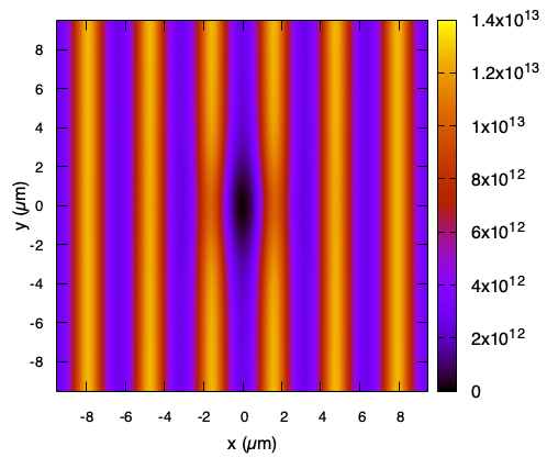
Figure 3: Structure of a singly-quantized vortex at x=y=0, one of the stable sites at the density minimum, for the case $\tilde{V}=2$. The density is in units of $cm^{-3}$.

In general, we find that the stable vortex positions are at the sites of minimum density, i.e. at the locus of maxima of the external potential (see also the following Sections, where different types of optical lattices are employed), in agreement with earlier observationsduine . In the case of the present one-dimensional lattice potential the stable positions correspond to the set of lines in the y direction (or better planes if we consider also the z direction) where the density is minimum. Therefore these lines are at the bottom of a kind of channels along which a vortex can freely move with no change of energy.

The equilibrium vortex structure at one of such sites is shown in Fig.3 for the case $\tilde{V}=2$. The streamlines for the velocity field $\vec{v}=\hbar\nabla\phi/m$ ($\phi$ being the phase of the wavefunction) are shown in Fig.4. Notice the strong deformations with respect to the circular patterns expected from a vortex in a homogeneous system. In order to display these deformations more clearly in Fig.5 we also show the streamlines of the modified phase ${\tilde{\phi}}$ as defined in Eq.(8) further on. ${\tilde{\phi}}$ represents the deviation of the phase from the imprinted phase in Eq.(7).

Figure 4: Streamlines for a vortex in the one-dimensional lattice, for the case $\tilde{V}=2$. The x and y axis show coordinates in $\mu$m.

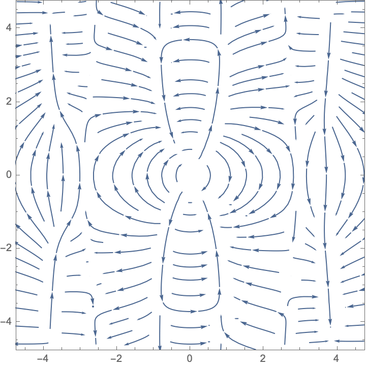
Figure 5: Streamlines of $\vec{\nabla}\tilde{\phi}$ for a vortex in the one-dimensional lattice, for the case $\tilde{V}=2$. The x and y axis show coordinates in $\mu$m.

Besides the stable positions at the bottom of the low density channels, there are also metastable positions at the density maxima, with higher energy than the equilibrium one. The associated energy barrier for vortex migration from one channel to the neighboring one depends on the amplitude of the modulation.

In Table 2 the vortex excitation energy and the energy barrier, both per particle and per unit length of the vortex, as well as the angular momentum are reported for selected values of $\tilde{V}$. The vortex excitation energy $\Delta E_{v}$ is finite because the computation box is finite (in an infinite system $\Delta E_{v}$ would diverge with the size of the system in a logarithmic way). $\Delta E_{v}$ in the modulated system is smaller than in the uniform system and it decreases for increasing $\tilde{V}$ because the vortex core is located in a region where the density decreases as $\tilde{V}$ increases. The energy barrier is a strongly increasing function of $\tilde{V}$ and this reflects the strong variation of the ratio $\rho_{max}/\rho_{min}$. We notice also the reduced value of the angular momentum and this reflects the reduced superfluid fraction in presence of the modulation. In the homogeneous state ($\tilde{V}=0$) the angular momentum deviates from the theoretical value $N\hbar$ due to the boundary effect of the computation box.

	$\tilde{V}\,\,\,\,$	$\Delta E_{v}/N$ ($nK/\mu m$)	$\,\,\,\,(E_{B}-E_{H})/N$ ($nK/\mu m$)	$\,\,\,\,<\hat{\mathcal{L}}_{z}>$ ($N\hbar$)
	$0$	$0.022$	-	$0.925$
	$2$	$0.018$	$0.0026\,$	$\,0.788$
	$4$	$0.011$	$0.0062\,$	$\,0.492$
	$7$	$0.005$	$0.0109\,$	$\,0.198$

Table 2: $\Delta E_{v}=(E_{H}-E_{0})/L_{z}$ is the energy (per unit length) cost to create a vortex in the minimum density sites, $E_{0}$ being the energy value (per atom) in the absence of the vortex; $(E_{B}-E_{H})/L_{z}$ is the energy barrier (per unit length) to move a vortex across the maximum density ridge; $<\hat{\mathcal{L}}_{z}>$ is the angular momentum along the z-axis in units of $N\hbar$.

III.2 Vortex dipole properties

Due to the presence of particular stable sites for a vortex caused by the presence of the spatial periodicity imposed by the optical lattice potential, a number of properties are expected to differ from those in a (nearly homogeneous) superfluid.

In classical hydrodynamics of incompressible fluids, a vortex dipole is a stable entity that moves with a constant velocity that is perpendicular to the plane defined by the vortex axis and the vector $\vec{l}$ joining the vortex and the antivortex core positions and inversely proportional to the distance $l$ between them. The same behavior holds in superfluid systemsdonnelly ; roberts when $l$ is much larger than the healing length, and the vortex dipole propagates with a constant velocity $v_{d}=\hbar/(ml)$. For example, in the absence of any modulation, a vortex-antivortex pair separated by a distance equal to $l=4d=12.7\,\mu m$ is found to translate with a constant velocity $0.058\pm 0.002$ $\mu m/ms$ (the error bar being estimated from the fit to the calculated data), to be compared with the hydrodynamical theoretical value $v_{d}=0.057$ $\mu m/ms$.

We have studied the real-time evolution of a vortex dipole imprinted in the superfluid in a 1D optical lattice described above. The position of the vortex core is located at each time step by carefully scanning the spatial mesh to find the minimum in the density corresponding to the vortex core. In particular, we will consider two different initial states for the vortex-antivortex pair, i.e. (i) the vortices are located in different minimum energy channels, at initial positions $x=\pm 2d$, where $d$ is the lattice constant; (ii) the vortices are located in the same channel (at $x=0$), at initial positions $y=\pm 2d$.

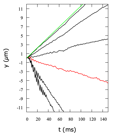
Figure 6: Trajectories along $y$ of a dipole with the vortices in two different channels. The vortices are initially set at positions $x=\pm 2d$ and with the same $y$. The $y$ coordinates of the two vortices of the dipole remain equal at all times within the grid of the computation. From top to bottom: $\tilde{V}=0,1,2,3,4,6,7$.

In the case (i) we find that the vortex pair move with a roughly constant velocity, the two vortices remaining in the same initial channel. The translation velocity decreases as the intensity $\tilde{V}$ increases until between $4$ and $6$ the velocity changes sign, i.e. it is in the opposite direction of motion compared to that of the homogeneous superfluid. This is shown in Fig.6. This is a novel effect not seen before. Superimposed on the translation is a weak oscillation for small values of $\tilde{V}$ but the oscillation becomes very intense for large values of $\tilde{V}$, for the largest intensity the motion periodically changes direction. The period of this oscillation becomes shorter for increasing $\tilde{V}$. For $\tilde{V}=7$ the period is about $1.9\,ms^{-1}$. We will discuss more quantitatively the origin of some of these effects in the following.

This behavior of the dynamics of the vortex dipole in distinct channels appears to be quite general: a) we have verified this when the vortex and the anti vortex lie in farther apart channels, b) when the vortex and the anti vortex start with a different $y$ coordinate they rapidly synchronize their motion at a common $y$ coordinate, i.e. they minimize their distance remaining in the initial channels.

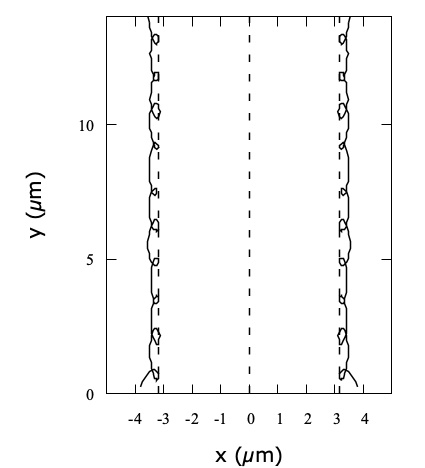
Figure 7: Dynamics of a vortex dipole when the initial vortex positions are slightly displaced with respect to the channel axis. The three vertical lines show the locii of minimum density. The simulation refers to the case $\tilde{V}=2$.

A rather peculiar behavior occurs when the initial positions of the two vortices in different channels do not coincide with the stable positions at the density minima, but are rather slightly displaced with respect to it, in opposite directions. During the ensuing dynamics, the vortices are found to move along the channels with complex trajectories shown in Fig.7. Such trajectories are the result of a uniform translation along the $y$ direction and of two oscillatory motions (occurring with the same frequency) along x and y directions. It should be stressed that this oscillatory motion perpendicular to the direction of translation is not an oscillatory motion around the position of minimum energy but it is rather a one-side oscillation: if the vortex starts to the right of the minimum at all times it remains on this side of the minimum and it never crosses to the other side. The same holds it it starts to the left. Therefore this dynamics is quite distinct from that of a massive particle moving around a minimum energy position.

In the case (ii), vortex and anti-vortex started in the same channel, for $\tilde{V}=4,7$ the two vortices moves towards one another, remaining in the same channel, until they annihilate at the origin, as shown in Fig.8. However, in the case of a less modulated structure ($\tilde{V}=2$), they remain initially in the same channel and move towards one another until they nearly touch at time $t=32\,ms$ (still being in the density minimum same channel): at this point, they appear to repel each other and jump to the next channel, annihilating there at a later time. We notice that a similar behavior has been observed in experimentsneely , where vortices in BEC are found to approach each other so closely that they appear to coalesce, but then move away from each other after the close encounter. This combination of jump and approach of the vortex pair two vortices of the dipole has some similarity with what we find in the case of 2D modulations as described in the next subsection.

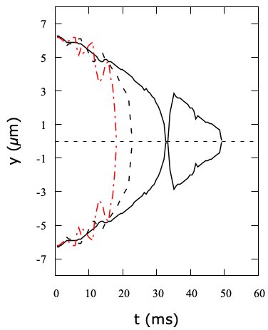
Figure 8: Trajectories along y of the two vortices of a dipole started in the same channel. The vortices are initially set at positions $y=\pm 2d$. From left to right $\tilde{V}=7,4,2$.

From the equation for the velocity of a vortex within the GP equation we can understand at a qualitative level some aspects of our results. The flow field of one vortex on the other is in the transverse direction of the channel, i.e. in the region where the density of the superfluid is increasing. This variation of density gives rise to a component of the velocity of the vortex in the longitudinal direction along the bottom of the channel. Following Ref.simula we write the vortex wave function $\psi_{v}(\vec{r},t)$ with the core located at position $\vec{r}_{0}$ at time $t$ as

$$\psi_{v}(\vec{r},t)=(x+iy-x_{0}-iy_{0})\tilde{\rho}e^{i\tilde{\phi}}$$ (8)

where $\tilde{\rho}(\vec{r},t)$ and $\tilde{\phi}(\vec{r},t)$ represent deviations of the modulus and of the phase from the ideal gas form, the first factor in eq.(8). $\tilde{\rho}(\vec{r},t)$ and $\tilde{\phi}(\vec{r},t)$ contain the following effects: the contribution due to the presence of other vortices, the effect of an external potential and, finally, the deviation of the $\psi_{v}$ from the ideal gas form due to the inter-atomic interactions. On the basis of the Gross-Pitaevskii equation here adopted the velocity of the vortex is simula

$$\tilde{\vec{v}}\equiv\frac{\hbar}{m}(\nabla\tilde{\phi}-\hat{\kappa}\times\nabla log\tilde{\rho})$$ (9)

where the vector $\hat{\kappa}$ is the unit vector in the direction of the circulation, i.e. in the z direction in the present case. As soon as the vortex position moves out of the bottom of the channel the second contribution to the velocity in Eq.(9) becomes non-zero due to the increasing density and its gradient is in the x direction. The vector product of these two vectors is in the y direction and points toward the other vortex. Therefore the velocity of one vortex of the pair has one longitudinal contribution from the external potential and a transverse contribution from the gradient of the phase due to the other vortex of the pair. This transverse term might dominate if the amplitude of the external potential is weak enough so that the vortex pair could move across channels but in any case due to the longitudinal contribution the two vortices move also against each other until they annihilate. The longitudinal contribution to the vortex velocity might dominate for large amplitude of the external potential so that the two vortices remain in the starting channel until annihilation. Eq.(9) for the velocity of the vortex core also explain why we see one-side oscillations of the vortex: the gradient of the local density tends to bring the vortex core toward the minimum density position but at this minimum this contribution to the velocity vanishes.

On the basis of Eq.(9) for the velocity of a vortex we can also understand why the translation velocity of the vortex dipole lying in two different channels is reduced with respect to the homogeneous case. In fact from Fig.5 one can see that the direction of ${\nabla\tilde{\phi}}$ along the line corresponding to $y=0$ has the opposite direction of the one of the homogeneous case, i.e. it points downward for $x>0$ and upward for $x<0$ and not vice versa as should be for a positive circulation vortex in a homogeneous superfluid. This means that the induced velocity due to the other vortex of the dipole is reduced compared with the value for the homogeneous system. Why the translation velocity even changes direction at large modulations and a longitudinal oscillation is present, however, cannot explained by these simple considerations.

III.3 Single vortex in a trap

An important question is if the oscillations in the dynamics of a vortex pair displayed in Fig.7 are a consequence of the mutual coupling between vortex-antivortex or are rather a property of the single vortex. We therefore considered the dynamics of a single vortex initially imprinted in a position slightly displaced from a position of minimum energy by the same amount as in the dipole simulation just described. However boundary effects mask the genuine dynamics in the case of an extended system with anti-periodic boundary conditions. To avoid this we used instead a finite system confined in the x-y plane by an additional circular ”box” potential of the form

$$V_{box}(x,y)=U_{0}(1-\frac{1}{e^{(R-R_{0})/\sigma}+1})$$ (10)

where $R=\sqrt{x^{2}+y^{2}}$, $R_{0}$ is the chosen value for the radius of the circular trap. We chose the following values: $R_{0}=14.3\,\mu m$, $U_{0}=60\,nK$, and $\sigma=0.212\,\mu m$. With such choice, the potential $V_{box}$ becomes different from zero as $R$ approaches $R_{0}$ and rapidly becomes very repulsive reaching the value $U_{0}$. As a result, the system is essentially unaffected in the inner region by this potential, where the system density is very close to that of the extended system, and goes exponentially to zero for radial distances from the center larger that $R_{0}$. We chose the number of atoms so that the density pattern in the interior of the circular trap is very similar to that of the extended system, for a given value of $\tilde{V}$.

We perform the computation with the external potential $V(\vec{r})=V_{OL}(x,y)+V_{trap}(x,y)$ and $V_{OL}$ is such that the center of the trap is a maximum of the OL, i.e. the center of the trap is an equilibrium position for the vortex core. We find that the vortex remains immobile if initially it is located at or very near the center of the trap, in the low density channel passing through it. If the initial position of the vortex is off-center along the y direction by a larger amount, however, the vortex is found to migrate towards the edge of the trap and disappears once it approaches the trap edge.

When the initial position is at $y=0$ but slightly off center along the x-direction, i.e. away from an equilibrium position, then the vortex moves toward the border of the trap and the radial motion is the superposition of a uniform motion in the radial direction and of a longitudinal and transverse oscillatory motion, similarly to the case of a vortex dipole shown in Fig.7. As in the case of the vortex dipole the oscillatory motion is one-sided: the vortex never crosses the line of minimum density but it remains on the same side of the channel from which it started. This is shown in Fig.9.

We have estimated, from the trajectories $x(t)$ and $y(t)$, the frequency characterizing these oscillations, which is reported in Fig.10 as a function of $\tilde{V}$, together with the average translation velocity of the vortex along the channel.

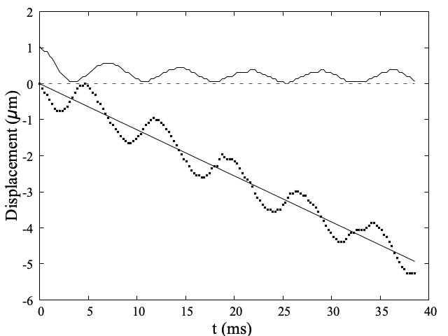
Figure 9: Upper curve: displacement $x(t)$ of the vortex core perpendicular to the channel axis; lower curve: displacement $y(t)$ of the vortex core parallel to the channel axis. The dotted line shows a least-square fit to $y(t)$, The simulation refers to the case $\tilde{V}=2$.

We finally note that the frequencies found for the oscillations of a single vortex, as discussed above, agree with the ones found for the case of a vortex dipole propagating in parallel channels.

We have checked the effect of changing the density of the system on the oscillation frequency in Fig.10. We thus studied the dynamics of a vortex slightly displaced from the equilibrium position in the transverse direction x, as described before, but when the total number of atoms in the system is doubled (halved). We find that both the amplitude and frequency of the transverse oscillations are unaffected by the increased (decreased) density. Also the frequency of the back-and-forth oscillations along the channel axis is not changed, whereas its amplitude is reduced as the density increases.

A natural question is if these oscillations might be due to the coupling of the vortex motion with the phonon excitations in the system which can be created by the vortex motion through the system. However, this is not the case. In fact we have computed, by using the Bogoliubov-de Gennes approach, the dispersion relation perpendicular and parallel to the channel direction. The phonons propagating in a direction perpendicular to the channels, having a dispersion relation which flattens at the Brillouin zone boundary, are those with the highest density of states. Their frequencies are found to be anc_next in the range $0.12<\omega<0.4$ ms^-1 (corresponding to the range $7>\tilde{V}>2$), i.e. much smaller than the observed vortex oscillation frequencies.

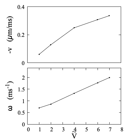
Figure 10: Upper panel: average translation velocity of a single vortex starting from a slightly displaced x-position from the center of the trap; Lower panel: calculated frequency of the oscillations occurring during the vortex motion along the channel.

IV ⁸⁷Rb in 2D optical lattice

IV.1 Square lattice

The external potential $V(\vec{r})$ acting on the Rb atoms is taken in the form of a periodic potential with square symmetry, i.e. $V({\bf r})=V_{OL}(x,y)$, where

$$V_{OL}(x,y)=V_{0}[cos^{2}(\kappa x)+cos^{2}(\kappa y)]$$ (11)

As done in the previous Sections, the optical potential strength $V_{0}$ is expressed in the following in terms of an adimensional quantity $\tilde{V}$ such that $V_{0}=\tilde{V}\times 10^{-14}$ Ha $=\tilde{V}\times 3.158\,nK$.

We first computed the ground-state in the presence of the periodic potential $V_{OL}$, for different values of the amplitude $\tilde{V}$.

We will use in the following a shorthand notation where the site of maximum density (corresponding to the minimum of the lattice potential) is called ’top’ (T), the site with minimum density (corresponding to the maximum of the lattice potential) is called ’hollow’ (H), and the saddle point between two adjacent top sites is called ’bridge’ (B).

As in the case of the 1D potential discussed in Section III, the system is superfluid, with a superfluid fraction $f_{s}$ which depends on the amplitude of the lattice modulation $V_{0}$. The relevant densities at the various lattice sites, and the calculated superfluid fraction are reported in Table 3.

	$\tilde{V}$	$\rho_{H}$ $(cm^{-3})$	$\rho_{T}$ $(cm^{-3})$	$\rho_{B}$ $(cm^{-3})$	$\mu(nK)$	$f_{s}$
	$0$	$6.943\times 10^{12}$	$6.943\times 10^{12}$	$6.943\times 10^{12}$	$2.584$	$1$
	$2$	$2.797\times 10^{12}$	$1.338\times 10^{13}$	$6.462\times 10^{12}$	$8.48$	$0.929$
	$4$	$0.9412\times 10^{12}$	$2.079\times 10^{13}$	$5.295\times 10^{12}$	$13.57$	$0.768$
	$7$	$0.1668\times 10^{12}$	$3.151\times 10^{13}$	$3.329\times 10^{12}$	$19.97$	$0.513$
	$9$	$0.0537\times 10^{12}$	$3.793\times 10^{13}$	$2.288\times 10^{12}$	$23.59$	$0.375$

Table 3: $\tilde{V}$ is the amplitude of the periodic potential; The density values at the Hollow, Top and Bridge sites are shown; $\mu$ is the chemical potential; $f_{s}$ is the superfluid fraction computed from the non-classical translational inertia.

	$\tilde{V}$	$\Delta E_{v}/N$ ($nK/\mu m$)	$(E_{B}-E_{H})/N$ ($nK/\mu m$)	$(E_{T}-E_{H})/N$ ($nK/\mu m$)	$<\hat{\mathcal{L}}_{z}>$ ($N\hbar$)
	$0$	$0.0220$	-	-	$\,0.925$ $(0.927^{\ast})$
	$2$	$0.0199$	$0.00049\,$	$0.00210$	$\,0.858$
	$4$	$0.0163$	$0.00046\,$	$0.00468$	$\,0.708$
	$7$	$0.0108$	$0.00026\,$	$0.00886$	$\,0.486$
	$9$	$0.0078$	$0.00019\,$	$0.01147$ $(unstable)$	$\,0.356$

Table 4: $\Delta E_{v}=(E_{H}-E_{0})/L_{z}$ is the energy (per unit length) cost to create a vortex in the minimum density (hollow) sites, $E_{0}$ being the energy value (per atom) in the absence of the vortex; $<\hat{\mathcal{L}}_{z}>$ is the angular momentum along the z-axis in units of $N\hbar$ (the value at $\tilde{V}=0$ denoted with an asterisk has been computed with a bigger cell, with a surface area in the x-y plane 4 times larger the one used for all the calculations; $(E_{B}-E_{H})/L_{z}$ and $(E_{T}-E_{H})/L_{z}$ are the energy barriers (per unit length) to move a vortex across the bridge site and the top site, respectively.

IV.2 Vortices

We imprint a single vortex using the procedure described before. If the vortex initial position is in a generic point of the unit cell of the modulating potential, during the imaginary time evolution the vortex core moves to the closest minimum density position. We find that stable vortex positions are at the low density sites corresponding to the maxima of the optical potential (hollow site), as discussed in the following. In the case of a square lattice these equilibrium positions have the same square symmetry. The vortex structure at the hollow site is shown in Fig.11 for the case $\tilde{V}=2$.

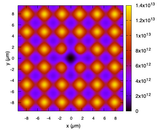
Figure 11: Structure of a singly-quantized vortex in the stable hollow site, for the case $\tilde{V}=2$. The vortex core is at the origin $(x=y=0)$. The density is in units of $cm^{-3}$.

We show in Figs.12 the equilibrium vortex structure for different values of the potential depth $\tilde{V}$, including the value $\tilde{V}=0$. In order to improve the visualization of the vortex core structure, we show in the figures the density differences with respect to the configuration without vortex.

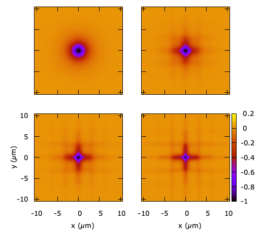
Figure 12: Relative density difference $(\rho_{vort}-\rho_{novort})/\rho_{novort}$ showing the minimum energy vortex structure (hollow site) for $\tilde{V}=0,2,4,7$.

We show in Fig.13 the calculated vortex excitation energy per unit length $\Delta E_{v}\equiv(E_{v}-E_{0})/L_{z}$ as a function of density of Rb atoms.

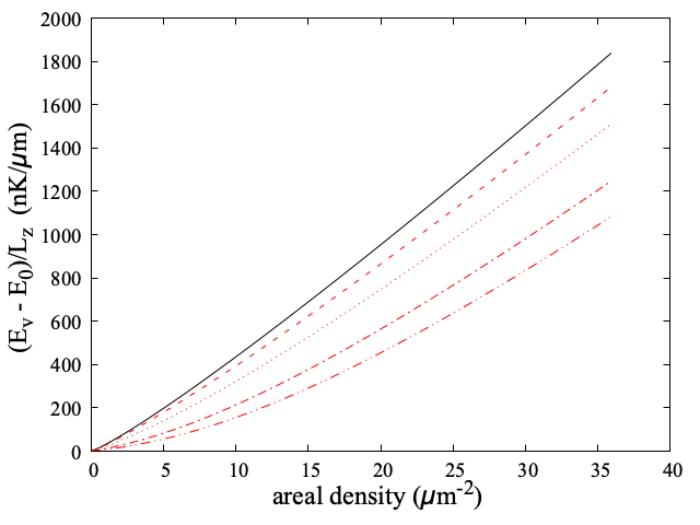
Figure 13: Vortex total energy as a function of the areal density of Rb atom. From top to bottom: $\tilde{V}=0,2,4,7,9$. The density $n_{a}=9.92\,\mu m^{-2}$ is the one used in most of the calculations discussed in the paper.

Notice the decrease of the vortex energy, for a given $N$, with the modulation amplitude of the lattice potential. This is a consequence of the decreasing density in the region of the vortex core as $\tilde{V}$ increases.

The streamlines around the vortex core are shown in Fig.14 for $\tilde{V}=7$.

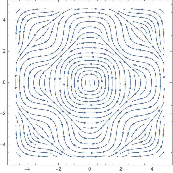
Figure 14: Streamlines for a vortex in the hollow site, for the case $\tilde{V}=7$. The x and y axis show coordinates in $\mu$m.

Besides the stable position at the hollow site, we have found that the saddle point between two adjacent density minima (bridge site in the following) is a metastable equilibrium position for a vortex, with slightly higher energy than the equilibrium one. A third metastable position for the vortex is found, at least for not too large value of $\tilde{V}$, at the high-density sites (top site in the following), corresponding to the minima of the optical potential. We show the vortex structures for these configurations in Fig.15, together with the stable hollow configuration.

In a uniform superfluid the energy of a vortex does not depend on the position of its core so that it is free to move under the influence of a perturbation. Our results show that in presence of a 2D optical lattice the vortex energy becomes a periodic function of position. The associated energy barriers for vortex migration along the lattice are reported in Table 4. These barriers will play an important role, as discussed in the following, in the dynamics of vortices across the lattice.

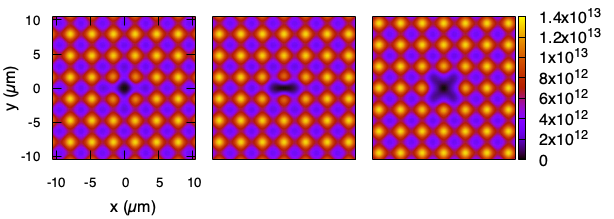
Figure 15: Structure of a singly-quantized vortex, for the case $\tilde{V}=2$ (only a portion of the density in the x-y plane is shown). From left to right: (i) hollow (most stable) site; (ii) bridge site; (iii) top site. The density is in units of $cm^{-3}$.

IV.3 Vortex dipole properties

Following the protocol described in Sect. III.B we imprint a vortex dipole in the 2D modulated superfluid and follow its real time dynamics. Instead of rigidly translating as in an homogeneous superfluid phase, in the presence of spatial modulation the vortex and antivortex approach each other by a series of jumps from one site to another moving mostly across the saddle positions until they annihilate in a very short time and their energy is released in the form of density wave excitations.

The path followed during the annihilation process depends on the amplitude $\tilde{V}$ of the optical lattice: the smaller the modulation, the farther the dipole moves along the y-direction before annihilation, and the longer it takes for the dipole to disappear. This is shown in Fig.16, where it appears that the vortex hopping occur mostly across bridge sites. The two vortices are initially placed at $x=\pm 2d=\pm 6.35\,\mu m$ (left panel of Fig.16). In the right panel of Fig.16 the annihilation paths are shown instead when the two vortices are initially placed at a larger mutual distance, $x=\pm 3d=\pm 9.53\,\mu m$. We recall that in absence of OL the vortex dipole would move rigidly with constant velocity in the $y$ direction.

It is of interest a comparison with the dynamics of a vortex dipole in the supersolid state of dipolar bosonsAnc21 . There is some similarity with what we find here in that the vortices of the dipole move by approaching each other by jumps between equilibrium sites with final annihilation but the studied case for dipolar atoms did not show any translation of the dipole in the direction perpendicular to the line joining the vortices.

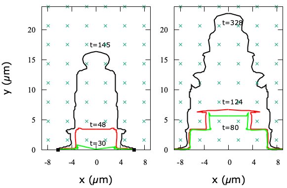
Figure 16: Trajectories of the two vortices of the dipole in the x-y plane ending in vortex dipole annihilation. Left panel: the two vortices are initially placed at $x=\pm 2d=\pm 6.35\,\mu m$. From top to bottom: $\tilde{V}=2,4,7$. The label on each trajectory gives the observed annihilation time in milliseconds. The crosses show the positions of the T sites where the Rb density is maximum. Right panel: the two vortices are initially placed at $x=\pm 3d=\pm 9.53\,\mu m$.

The energy released immediately after the annihilation goes into excitations of the system. In order to gain some insights on the character of the excitations we computed the spectral density of the kinetic energy of the superfluid velocity field, decomposing it into compressible and incompressible parts tsubota ; spectra ; bradley . Briefly, one splits the density-weighted velocity field $\vec{u}(\vec{r},t)\equiv\sqrt{\rho(\vec{r},t)}\vec{v}(\vec{r},t)$ into a compressible (C) and an incompressible (I) part, $\vec{u}(\vec{r},t)=\vec{u}^{I}(\vec{r},t)+\vec{u}^{C}(\vec{r},t)$, such that $\vec{\nabla}\cdot\vec{u}^{I}(\vec{r},t)=0$ and $\vec{\nabla}\wedge u^{C}(\vec{r},t)=0$. One can therefore decompose the kinetic energy $E$ into two parts, $E=E^{I}+E^{C}$, where

$$E^{I,C}=\frac{m}{2}\int d\vec{r}|\vec{u}^{I,C}(\vec{r},t)|^{2}$$ (12)

The compressible component is attributed to the kinetic energy contained in the sound field, while the incompressible part gives the contribution from quantum vortices.

In $\vec{k}$-space, the total incompressible (compressible) kinetic energy $E^{I,C}$ is given by

$$E^{I,C}=\frac{m}{2}\Sigma_{j=x,y}\int d^{2}\vec{k}|F_{j}(\vec{k})|^{2}$$ (13)

where

$$F_{j}(\vec{k})=\frac{1}{2\pi}\int d^{2}\vec{r}e^{-i\vec{k}\cdot\vec{r}}u_{j}^{I,C}(\vec{r})$$ (14)

(the time-dependence is implied).

The one-dimensional spectral density in $k$-space is given by integrating over the azimuthal angle

$$E^{I,C}(k)=\frac{mk}{2}\Sigma_{j=x,y}\int_{0}^{2\pi}d\phi_{k}|F_{j}(\vec{k})|^{2}$$ (15)

We show in Fig.(17) the spectral density of the kinetic energy, $E^{I,C}(k,t)$ for the case $\tilde{V}=4$, when the two vortices are initially placed at positions $x=\pm 2d$ (whose trajectories are displayed in the left panel of Fig.16. The horizontal arrows show two relevant wave vectors: $k_{vv}=2\pi/l$, where $l$ is the initial vortex-vortex distance, and $k_{d}=2\pi/d$, which is the wave vector corresponding to the periodic modulation with lattice constant $d$. The lower panel clearly shows the sharp transition when the vortices disappear with a strong drop of the incompressible kinetic energy. The peak in the incompressible part appearing below the wave-vector $k_{vv}$ before annihilation is a general feature also found in the calculations for a vortex dipole in Ref.bradley, (see in particular the Fig.3 of that reference). After vortex annihilation the compressible part (upper panel) starts showing features connected to density fluctuations (sound waves). One can notice that also before vortex annihilation a faint time modulation is present over an extended range of k vectors and its period is about 7 ms. We have computed anc_next the phonon frequencies of the Rb gas in presence of the 2D OL but without vortices and find that this 7 ms period falls inside a gap of the phonon spectrum. The vortex dipole represents a defect in the modulated system and our interpretation of this oscillation is in term of a localized vibration of the Rb gas around the moving vortex dipole.

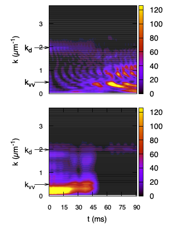
Figure 17: Kinetic energy spectra for the case $\tilde{V}=4$, square OL. Top: compressible part; bottom: incompressible part.

IV.4 Triangular and Honeycomb optical lattice.

We consider here two other lattice types, with triangular symmetry. The periodic potential mimics what is actually employed in experiment where a potential with triangular symmetry is created by three laser beams that intersect in the x–y plane mutually enclosing angles of 120^∘ with lattice vectors $\vec{k}_{1}$, $\vec{k}_{2}$ and $\vec{k}_{3}$ (see Ref.becker, ).

We use here the following form:

$$V^{tri}_{OL}=\tilde{V}\{\frac{4}{3}-\frac{4}{9}[cos(\vec{b}_{1}\cdot\vec{R})+cos(\vec{b}_{2}\cdot\vec{R})+cos((\vec{b}_{1}-\vec{b}_{2})\cdot\vec{R})]\}$$ (16)

where $\vec{R}=(x,y)$, $\vec{b}_{1}=\vec{k}_{2}-\vec{k}_{1}$, $\vec{b}_{2}=\vec{k}_{2}-\vec{k}_{3}$, and $\vec{k}_{1}=\kappa(\sqrt{3}/2,-1/2)$, $\vec{k}_{2}=\kappa(0,1)$, $\vec{k}_{3}=-\kappa(\sqrt{3}/2,1/2)$. $k$ is the wave vector of the laser employed for the lattice beams. Here $\kappa=4\pi/(3d)$, $d$ being the lattice constant (the same used in the square optical lattice). The numerical coefficients in the previous equations are such to give the same min-max excursion, $(0,2V_{0})$, of the square optical potential used in the previous sections. The number of Rb atoms $N$ is also chosen such to have the same mean density as in the square lattice case. The density of the Rb atoms is a periodic function of position with triangular symmetry.

A different symmetry of the density of the atoms can be obtained in the presence of the potential

$$V_{OL}^{hon}(x,y)=-V_{OL}^{tri}(x,y)+2V_{0}$$ (17)

so that the role of maxima and minima of $V_{OL}^{tri}(x,y)$ are exchanged. In this case the maxima in the Rb density will be at the points of an honeycomb lattice.

We have studied the vortex properties in these two cases. As in the case of the square lattice we find that the equilibrium positions of a vortex are at the sites of minimum density.

We show in Figs.(18) and (19) the equilibrium vortex structure for different values of the potential depth $\tilde{V}$, including the value $\tilde{V}=0$, in the triangular and honeycomb lattice, respectively. In order to facilitate the visualization, as done in Fig.(12), we show the density differences with respect to the configuration without vortex.

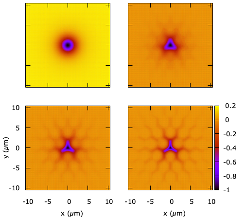
Figure 18: Relative density difference $(\rho_{vort}-\rho_{novort})/\rho_{novort}$ showing the minimum energy vortex structure (hollow site) in the triangular lattice for for $\tilde{V}=0,2,4,7$.

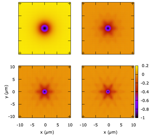
Figure 19: Relative density difference $(\rho_{vort}-\rho_{novort})/\rho_{novort}$ showing the minimum energy vortex structure (hollow site) in the honeycomb lattice for $\tilde{V}=0,2,4,7$.

Finally, we show in Fig.(20) and (21) the trajectories of a vortex-antivortex pair, obtained by solving the time-dependent equation (2), as they propagate through the lattice before undergoing annihilation after some time. Again, the propagation occurs in the form of jumps across the lower energy barrier sites, and the lower the modulation, the longer it takes for the annihilation to occur and the larger is the displacement of the dipole before annihilation. From these results and those for the square lattice we conclude that the basic features of the motion of a vortex dipole do not depend on the lattice symmetry and that the lifetime of the vortex dipole can be controlled by the intensity of the OL.

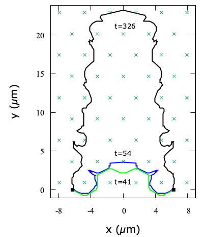
Figure 20: Trajectories in the x-y plane ending in the vortex dipole annihilation, for the triangular lattice. The two vortices are initially placed at $x=\pm 2d=\pm 6.35\,\mu m$. From top to bottom: $\tilde{V}=2,4,7$. The label on each trajectory report the observed annihilation time in milliseconds. The crosses show the positions of the T sites where the Rb density is maximum.

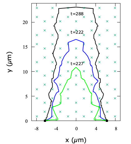
Figure 21: Trajectories in the x-y plane ending in the vortex dipole annihilation, for the honeycomb lattice. The two vortices are initially placed at $x=\pm 2d=\pm 6.35\,\mu m$. From top to bottom: $\tilde{V}=2,4,7$. The label on each trajectory report the observed annihilation time in milliseconds. The crosses show the positions of the T sites where the Rb density is maximum.

IV.5 Visualizing vortices in optical lattices

As previously discussed, the direct visualization of vortices in the system studied here might be difficult, especially for large values of the amplitude of the OL. This is a consequence of the fact that the vortex cores tend to localize in the low-density sites of the periodic lattice. We suggest here that a simple way to visually detect the presence of vortices in the modulated system can be achieved by sudden removal of the optical lattice potential.

One way to experimentally cause vortex nucleation is by means of rotation of the optical lattice. We consider here the the case of the square lattice with the same radial confining potential (circular ”box”) used to analyze the dynamics of a single vortex in the 1-dimensional lattice described in Section III.C.

To enforce rotations (with some fixed angular velocity $\omega$, around the z-axis) we work in the co-rotating frame, described by the Hamiltonian

$$\left\{H\,-\hbar\omega\hat{L}_{z}\right\}\,\Psi(\mathbf{r})=\,\mu\,\Psi(\mathbf{r})$$ (18)

where $\hat{\mathcal{L}}_{z}$ is the total angular momentum operator in the $z$-direction and $H$ is the Hamiltonian of Eq.(2).

We first compute the stationary state in the presence of a rotation of the system with constant $\omega$ by solving the Euler-Lagrange equations in imaginary time associated with the previous Hamiltonian. If the imposed angular velocity is large enough (i.e. larger than the critical frequency for a single vortex nucleation), a number of vortices will eventually populate the system, which may later be visualized. These vortices, as it happens in rotating finite superfluid samples, are initially nucleated on the boundaries of the system, and rapidly settle to an equilibrium position at a distance from the center which depends on the value of the rotational frequency: the larger the latter is, the closer to the center will be the vortices in the stationary-state configuration.

As an example, we show in the first panel of Fig.(22) the stationary state obtained with $\omega=2\pi\times 8$ Hz in presence of a square OL with value $\tilde{V}=7$. At first sight, the resulting density profile resembles that of the ground-state in the absence of rotation. However, a finite value for $\hat{\mathcal{L}}_{z}$ indicates the presence of vorticity in the system.

A possible way to increase the vortex visibility is to rapidly remove the periodic potential (but keeping the radial confinement active) so that the system may evolve towards a more homogeneous state where the increased contrast between the empty core and the background density may allow to reveal the vortex positions.

We therefore perform a real-time dynamics, starting from the stationary state shown in the first panel of Fig.22, with a linear ramp of the optical potential which brings its value from $\tilde{V}=7$ to zero in 5 ms. The three panel (from left to right, from top to bottom) of Fig.22 show snapshots of the Rb density during the real-time evolution, clearly showing a ring of six vortices as the density modulations are suppressed. Notice that the vortex core positions rotate with the imposed angular velocity $\omega$.

We remark that the time required to visually disclose the vortex cores is so short that the final core positions (last panel in the figure) coincide with their initial positions in the modulated phase shown in the first panel. Such short times exclude the possibility that vortices are nucleated during the quench from the modulated to the homogeneous phase.

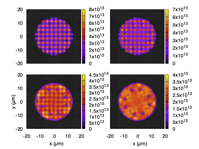
Figure 22: From left to right, from top to bottom: panel (1): density of the stationary state in the co-rotating frame, for $\tilde{V}=7$; panel (ii-iv): density patterns at $t=1.6$ ms, $t=4.1$ ms, and $t=6.4$ ms, during the time evolution of the state (1) when the amplitude $\tilde{V}$ is ramped linearly to zero in 5 ms. The density is in units of $cm^{-3}$.

V Conclusions

We have studied the superfluid phase of boson ⁸⁷Rb atoms under the influence of an optical potential which induces a spatial modulation of the local density. The main interest is on the static and dynamical properties of vortex excitations. We have studied the system at zero temperature with the mean field Gross-Pitaevskii equation and our investigation is mainly on the regime of strong modulation when the excursion between low and high density becomes quite large. We study the system in a flat geometry so that one can neglect the transverse direction and the system is close to the 2D limit. The dynamics of a vortex in an almost 2D superfluid is rather simple when no other vortex is present within its healing length: the core moves with the gradient of the phase due to other vortices. Consequences of this law are, for instance, that a vortex dipole is a stable entity and it rigidly translates with constant velocity and that one vortex in a circular trap performs a procession around the trap center. Deviations from such behaviors in a weakly inhomogeneous superfluid have been studied by a number of authors as discussed in the Introduction. We have studied a rather different regime, when the inhomogeneity is very large. In presence of an intense optical potential we find a vortex behavior quite different from that of the uniform superfluid. Depending on the symmetry of the optical lattice two vortices of opposite chirality, a vortex dipole, can move by jumps approaching each other until annihilation with a lifetime of the pair depending on the intensity of the optical lattice or the vortices of the dipole do translate but with a velocity even of opposite direction of that present in the uniform case and, in addition, this translation takes place together with an oscillatory motion. Or a single vortex in a trap does not perform a processional motion but it move toward the periphery of the trap with a complex motion consisting of translation and of an oscillation. These periodic motions are single-side in the sense that they never cross the equilibrium position from the starting place, a behavior quite different from that of a massive particle around an equilibrium position. Such features of the vortex motion derive from two facts, on one hand the vortex energy depends on the local density at the position of its core and the energy is lowest where the density has a minimum, I.e. at the positions of the maxima of the optical lattice.

A consequence of this is that a vortex is not free to move but it is pinned to specific sites or lines depending on the symmetry of the optical lattice. On the other hand the stream lines have large deviations from the simple circular shape of the uniform superfluid. The superfluid fraction is reduced from unity, even if our system is at zero temperature, and this reduction can be quite large for large amplitudes of the optical potential. In the case of 1D optical potential the superfluid has a stripe structure and the superfluidity is very anisotropic: the superfluid fraction is unity along the stripes and it is reduced in the direction perpendicular to the stripes. At the same time a vortex has a unit circulation but a reduced angular momentum compared to that of a uniform superfluid.

It is possible now to generate experimentally vortex dipoles in a superfluid of cold atoms kwon so it should be possible to verify our predictions for the dynamics of vortices in a modulated superfluid. We have studied the case of ⁸⁷Rb atoms but our results should be valid for other bosons with positive scattering length. The jumping behavior and annihilation of a vortex dipole seen in the case of a 2D optical lattice have some similarity with that of a vortex dipole in a supersolid Anc21 .

Our study is based on a mean field theory and we should pose the question of the accuracy of such theory because it is known that a Mott transition to a localized state sets in when the optical lattice is strong enough greiner . In terms of recoil energy the amplitude of the optical potential in our study is much smaller of the amplitudes for which experimentally the localization has been found to set in. In addition we have indication of the internal consistency of the used theory because we have performed computations anc_next of the excitation spectrum of our system with the Bogoliubov-de Gennes equation and no sign of instability has been found. This gives confidence on our theoretical results.

We have been able to explain at a qualitative level some aspects of our results like the approach of the two vortices of a dipole or the one sided oscillations in terms of the expression of the velocity of the vortex core and its relation to the gradient of the local density of the superfluid.

One would like to see a treatment of the systems of our study on the basis of an approximate analytic treatment like a suitable extension of the point-vortex approximation as explored in Ref.simula, . Different extensions of the present study come to mind. One is the study of vortices in the supersolid phase of soft core bosons or in supersolid with a stripe structure. The flat geometry used in our computations does not allow flexural motion of the core of the vortex. Of interest will be a similar study when the system is extended in the third direction and key questions are the fate of the Kelvin waves that characterize the motion of a vortex core in 3D donnelly or if additional excitations are present similar to kinks of a dislocation in a solid. Theory predicts that a supersolid phase with a stripe structure can be present with dipolar bosons ripley . Our results for the vortex behavior in a 1D modulated system should be relevant also for such supersolid system.

- (1) R.J. Donnelly, Quantized vortices in helium II, Cambridge University Press (1991).
- (2) A.L. Fetter, Rev. Mod. Phys. 81, 647 (2009).
- (3) S. Burger, F.S. Cataliotti, C. Fort, P. Maddaloni, F. Minardi and M. Inguscio, Europhys. Lett. 57, 1 (2002); F.S. Cataliotti, S. Burger, C. Fort, P. Maddaloni, F. Minardi, A. Trombettoni, A. Smerzi and M. Inguscio, Science 293, 843 (2001).
- (4) J. Tao, M. Zhao and I.B. Spielman, Phys. Rev. Lett. 131, 163401 (2023).
- (5) A.J. Leggett, Phys. Rev. Lett. 25, 1543 (1970); A.J Leggett, J. Stat. Phys. 93, 927 (1998).
- (6) S. Moroni, F. Ancilotto, P. L. Silvestrelli and L. Reatto, Phys. Rev. B 103, 174514 (2021).
- (7) L. Chomaz, I. Ferrier-Barbut, F. Ferlaino, B. Laburthe-Tolra, B.L. Lev and T. Pfau, Reports on Progress in Physics 86, 026401 (2022).
- (8) T. Isoshima, M. Nakahara, T. Ohmi, and K. Machida, Phys. Rev. A 61, 063610 (2000); K. C. Wright, L. S. Leslie, A. Hansen, and N. P. Bigelow, Phys. Rev. Lett. 102, 030405 (2009).
- (9) T.W. Neely, E.C. Samson, A.S. Bradley, M.J. Davis and B.P. Anderson, Phys. Rev. Lett. 104, 160401 (2010).
- (10) Y.-J. Lin, R.L. Compton, K. Jimenez-Garcia, J.V. Porto and I.B. Spielman, Nature Letters 462, 628 (2009).
- (11) W.J. Kwon, G. Del Pace, K. Xhani, L. Galantucci, A.M. Falconi, M. Inguscio, F. Scazza and G. Roati, Nature 600, 64–69 (2021).
- (12) P.G. Kevrekidis et al., J. Phys. B: At. Mol. Opt. Phys. 36, 3467 (2003).
- (13) D.S. Goldbaum and E.J. Mueller, Phys. Rev. A 77, 033629 (2008).
- (14) H. Pu, L.O. Baksmaty, S. Yi and N.P. Bigelow, Phys. Rev. Lett. 94 190401 (2005); K. Kasamatsu and M. Tsubota, Phys. Rev. Lett. 97 240404 (2006).
- (15) E.A. Ostrovskaya and Y.S. Kivshar, Phys. Rev. Lett. 93, 160405 (2004); T.J. Alexander, E.A. Ostrovskaya, A.A. Sukhorukov and Y.S. Kivshar, Phys. Rev. A 72, 043603 (2005).
- (16) E. Poli, T. Bland, S.J.M. White, M.J. Mark, F. Ferlaino, S. Trabucco and M. Mannarelli, Phys. Rev. Lett. 131, 223401 (2023).
- (17) A. Gallemi, S.M. Roccuzzo, S. Stringari and A. Recati, Phys. Rev. A 102, 023322 (2020).
- (18) A. Gallemi and L. Santos, Phys. Rev. A 106, 063301 (2022).
- (19) E. Casotti, E. Poli, L. Klaus et al., arXiv:2403.18510v1 (2024).
- (20) F. Ancilotto, M. Barranco, M. Pi, and L. Reatto, Phys. Rev. A 103, 033314 (2021).
- (21) J.W. Reijnders and R.A. Duine, Phys. Rev. Lett. 93, 060401 (2004); S. Tung, V. Schweikhard and E. A. Cornell, Phys. Rev. Lett. 97, 240402 (2006); H. Pu, L. O. Baksmaty, S. Yi, and N. P. Bigelow, Phys. Rev. Lett. 94, 190401 (2005).
- (22) A. Marte, T. Volz, J. Schuster, S. Durr, G. Rempe, E. G. M. van Kempen, and B. J. Verhaar, Phys. Rev. Lett. 89, 283202 (2002).
- (23) A. Ralston and H. S. Wilf, Mathematical methods for digital computers (John Wiley and Sons, New York, 1960).
- (24) Y. Pomeau and S. Rica, Phys. Rev. Lett. 72, 2426 (1994); N. Sepulveda, C. Josserand, and S. Rica, Eur. Phys. J. B 78, 439 (2010).
- (25) M. Pi, R. Mayol, A. Hernando, M. Barranco, and F. Ancilotto, J. Chem. Phys. 126, 244502 (2007).
- (26) M. Sadd, G. V. Chester, and L. Reatto, Phys. Rev. Lett. 79, 2490 (1997).
- (27) F. Ancilotto, M. Barranco and M. Pi, Phys. Rev. B 97, 184515 (2018).
- (28) A.J. Groszek, D.M. Paganin, K. Helmerson and T.P. Simula, Phys. Rev. A 97, 023617 (2018).
- (29) C.A. Jones and P.H. Roberts, J. Phys. A 15, 2599 (1982); A. Griffin, V. Shukla, M.-E. Brachet, and S. Nazarenko, Phys. Rev. A 101, 053601 (2020).
- (30) F. Ancilotto, unpublished.
- (31) M. Tsubota, K. Fujimoto, S.Y. Tsubota, J. Low. Temp. Phys. 188, 119 (2017).
- (32) C. Nore, M. Abid, and M.E. Brachet, Phys. Fluids 9, 2644 (1997).
- (33) A.S. Bradley and B.P. Anderson, Phys. Rev. X 2, 041001 (2012).
- (34) C. Becker, P. Soltan-Panahi, J. Kronjager, S. Dorscher, K. Bongs and K. Sengstock, New Journal of Physics 12, 065025 (2010).
- (35) M. Greiner, M.O. Mandel, T. Esslinger, T. Hansch and I. Bloch, Nature 415, 39 (2002).
- (36) B.T.E. Ripley, D. Baillie and P.B. Blakie, Phys. Rev. A 108, 053321 (2023).