Clio: Real-time Task-Driven Open-Set 3D Scene Graphs

Abstract

Modern tools for class-agnostic image segmentation (e.g., SegmentAnything) and open-set semantic understanding (e.g., CLIP) provide unprecedented opportunities for robot perception and mapping. While traditional closed-set metric-semantic maps were restricted to tens or hundreds of semantic classes, we can now build maps with a plethora of objects and countless semantic variations. This leaves us with a fundamental question: what is the right granularity for the objects (and, more generally, for the semantic concepts) the robot has to include in its map representation? While related work implicitly chooses a level of granularity by tuning thresholds for object detection and association, we argue that such a choice is intrinsically task-dependent. The first contribution of this paper is to propose a task-driven 3D scene understanding problem, where the robot is given a list of tasks, specified in natural language, and has to select the granularity and the subset of objects and scene structure to retain in its map that is sufficient to complete the tasks. We show that this problem can be naturally formulated using the Information Bottleneck (IB), an established information-theoretic framework to discuss task-relevance. The second contribution is an algorithm for task-driven 3D scene understanding based on an Agglomerative IB approach, that is able to cluster 3D primitives in the environment into task-relevant objects and regions, and executes incrementally. The third contribution is to integrate our task-driven clustering algorithm into a real-time pipeline, named Clio, that constructs a hierarchical 3D scene graph of the environment online and using only onboard compute, as the robot explores it. Our final contribution is an extensive experimental campaign showing that Clio not only allows real-time construction of compact open-set 3D scene graphs, but also improves the accuracy of task execution by limiting the map to relevant semantic concepts.

I Introduction

Figure 1: We propose Clio, a novel approach for building task-driven 3D scene graphs in real-time with embedded open-set semantics. We draw inspiration from the classical Information Bottleneck principle to form task-relevant clusters of object primitives given a set of natural language tasks —such as ”Read brown textbook”— and by clustering the scene into task-relevant semantic regions such as “Kitchenette” or “Workspace”.

A fundamental problem in robotics is to create a useful map representation of the scene observed by the robot, where usefulness is measured by the ability of the robot to use the map to complete tasks of interest [1, 2]. Recent works, including [3, 4, 5, 6, 7], build metric-semantic 3D maps by detecting objects and regions corresponding to a closed set of semantic labels. However, closed-set detection is inherently limited in terms of the set of concepts that can be represented and does not cope well with the intrinsic ambiguity and variability of natural language. In order to overcome these limitations, a new set of approaches [8, 9] has begun to leverage vision-language foundation models for open-set semantic understanding. These approaches use a class-agnostic segmentation network [10] (SegmentAnything or SAM) to generate fine-grained segments of the image and then apply a foundation model [11] to get an embedding vector describing the open-set semantics of each segment. Objects are then constructed by associating segments whenever their embedding vectors are within a predefined similarity threshold. These approaches, however, leave to the user the difficult task of tuning suitable thresholds to control the number of segments that are extracted from the scene as well as the threshold used to decide whether two segments have to be clustered together. More importantly, these methods do not capture intuition that the choice of semantic concepts in the map is not just driven by semantic similarity, but it is intrinsically task-dependent.

For example, consider a robot tasked with moving a piano across a room. The robot gains almost no value by distinguishing the location of all the keys and strings, but can instead complete the task by considering the piano as one large object. On the other hand, a robot tasked with playing the piano must consider the piano as many objects (i.e., the keys). A robot tasked with tuning the piano must view the piano as even more objects — considering the strings, tuning pins, and so forth. Likewise, questions such as if a pile of clothes should be represented as a single pile or as individual clothes, or if a forest should be represented as single area of landscape or as branches, leaves, trunks, etc., remains ill-posed until we specify the tasks that the representation has to support. Humans not only take into account the task when (consciously or unconsciously) deciding which objects to represent and how, but are also able to consequently ignore parts of a scene that are irrelevant to the task [12].

Contributions. Our first contribution (Section III) is to state the task-driven 3D scene understanding problem, where the robot is given a list of tasks, specified in natural language, and is required to build a minimal map representation that is sufficient to complete the given tasks. More specifically, we assume the robot is capable of perceiving task-agnostic primitives in the environment, in the form of a large set of 3D object segments and 3D obstacle-free places, and has to cluster them into a task-relevant compressed representation which only contains relevant objects and regions (e.g., rooms). This problem can be naturally formulated using the classical Information Bottleneck (IB) [13] theory, which also provides algorithmic approaches for task-driven clustering.

Our second contribution (Section IV) is to apply the Agglomerative IB algorithm from [14] to the problem of task-driven 3D scene understanding. In particular, we show how to obtain the probability densities required by the algorithm in [14] using CLIP embeddings, and show that the resulting algorithm can be executed incrementally as the robot explores the environment, with a computational complexity that does not increase with the environment size.

Figure 2: Clio generates a 3D scene graph in real-time using a laptop carried by Spot. We show that Spot is able to execute grasping commands, expressed in natural language, using Clio’s task-driven 3D scene graph.

Our third contribution (Section V) is to include the proposed task-driven clustering algorithm into a real-time system, named Clio (Fig. 1). Clio takes a list of tasks specified in natural language at the beginning of operation: for instance, these can be the tasks the robot is envisioned to perform during its lifetime or during its current deployment. Then, as the robot operates, Clio creates a hierarchical map, namely a 3D scene graph, of the environment in real-time, where the representation only retains task-relevant objects and regions. Contrary to current approaches for open-set 3D scene graph construction (e.g., [9]) which are restricted to off-line operation when querying large vision-language models (VLMs) [15] and Large Language Models (LLMs) such as [16], Clio runs in real-time and onboard and only relies on lightweight foundation models, such as CLIP [11].

We demonstrate Clio on the Replica dataset [17] and in four real environments (Section VI) — an apartment, an office, a cubicle, and a large-scale building scene. We also show real-time onboard mapping with Clio on a Boston Dynamics Spot quadruped with a robotic arm (Fig. 2). Clio not only allows real-time open-set 3D scene graph construction, but also improves the accuracy of task execution by limiting the map to relevant objects and regions.

We release Clio open-source at https://github.com/MIT-SPARK/Clio along with our custom datasets.

II Related Work

Foundation Models in Robotics and Vision. The recent emergence of vision-language models [11, 18, 15] and large language models [16] has led to numerous works exploring their potential for 3D scene understanding [19, 20] and robot planning [21, 22, 23]. Multiple works have surveyed the state of the art in foundation models along with their limitations [24, 25, 26, 27, 28]. Class-agnostic segmentation networks [10, 29] have been coupled with foundation models to enable open-set image segmentation [30, 31, 32, 33, 34, 35]. Recent works have also explored direct class-agnostic 3D segmentation [36]. Saliency detection has been used to identify parts of an image that a human would likely notice first [37]. Here, instead of visual saliency, we desire to create task-driven maps of a scene.

Foundation Models for 3D Mapping. Recent work has coupled foundation models with neural radiance fields [38] and Gaussian Splatting [39]. Kerr et al. [40] propose LERF, which constructs a radiance field that can render dense CLIP vectors of the scene. LERF can be queried via text and estimate which parts of the scene are most similar to the query using an augmented cosine similarity score. Qin et al. [41] develop LangSplat which builds upon LERF by using Gaussian Splatting to create a 3D scene language map with a substantial speedup. Blomqvist et al. [42] develop an approach to incrementally construct a neural semantic map for SLAM. Kim et al. [43] construct a hierarchical neural map that renders at different levels of granularity, clustering and dividing objects into parts. Taioli et al. [44] use CLIP to construct an implicit grid map that can be queried via text.

Several works incorporate open-set detection into 3D maps of a scene [45, 46, 47, 48, 49, 50]. Chang et al. [51] perform open-vocabulary mapping combined with a graph neural network trained on a closed set to map objects and their relationships. Takmaz et al. [52] develop a method for open-set instance segmentation. Jatavallabhula et al. [8] generate a semantic 3D point cloud where CLIP vectors are assigned to each point. Most similar to ours is ConceptGraphs [9], which constructs a 3D graph of objects with edges connecting objects via their relationships as assigned with an LLM [16]. ConceptGraphs uses CLIP and SAM to cluster a scene into objects defined by their semantic and geometric similarity to each other. Optionally, ConceptGraphs queries a large vision-language model [15] using multiple views of each object to compute a succinct description of the object. Objects can be then queried either with cosine similarity via CLIP or with the LLM.

Task-Driven Representations. The classical Information Bottleneck (IB) [13] aims to compress a given signal while preserving the mutual information between the compressed representation and another signal of interest. The initial work [13] has been extended into a bottom-up clustering method known as the Agglomerative IB [14]. We build on IB theory with the goal of compressing a scene representation into clusters of relevant objects and regions for a given set of tasks. Gordon et al. [53] extend the Information Bottleneck to compress a set of individual images into clusters such that each cluster preserves information about the context of the images contained in the cluster. Wang et al. [54] use the IB principle for attribution between image and text inputs of VLMs with experiments performed with CLIP. Larsson et al. [55, 56] leverage the Agglomerative IB to obtain an optimal map compression for agents with limited resources.

Soatto and Chiuso [1] derive expressions for minimally sufficient scene representations that preserve relevant information about some task of interest, and [57] develops theory around constructing foundation models of physical scenes. Eftekhar et al. [58] compress visual observations in a task-relevant manner. Their work uses a learned codebook module that takes in a current agent’s action along with the task and sensor data, and outputs an action to step towards the goal for navigation. Another line of work detects regions of interest in images based on affordances [59] and creates 3D maps of affordances of objects in a scene [60].

III Problem Formulation:
Task-Aware 3D Scene Understanding

While many researchers would agree that a map representation has to be task-dependent, to date there is no general framework to establish what is the right granularity for the semantic concepts included in the robots’ metric-semantic 3D map. This gap has been partially motivated by the difficulty of providing rich task descriptions, with the result that existing task-driven representation frameworks in vision and robotics are either too narrow or too computationally expensive [61].

In this paper, we leverage two key insights. First of all, progress in vision-language models has brought together visual information and text descriptions in a way that was not possible before. This greatly simplifies the problem of task description: we can just state the task as a list of language instructions the robot is expected to execute during its lifetime or during its current deployment (e.g., “wash the dishes”, “fold the clothes”, “pick up toys and place them on the shelves”) and use VLMs to relate these instructions to visual data. Below, we denote the list of tasks with the symbol $Y$. Second, modern foundation models for task-agnostic segmentation provide a way to over-segment an image into a potentially large number of segments, which we can reproject to 3D. Similarly, using geometric segmentation techniques, we can easily segment environments into a large number of obstacle-free places [6]. In the following, we refer to the task-agnostic 3D segments and places as task-agnostic primitives and denote them with $X$; intuitively, these provide a superset of the concepts we want to retain in our map.

Using these insights we formulate task-aware 3D scene understanding as the problem of compressing the task-agnostic primitives $X$ into a cluster of task-relevant concepts $\tilde{X}$, which are maximally informative about the tasks $Y$. This naturally leads to the Information Bottleneck principle.

Task-Aware 3D Scene Understanding as an Information Bottleneck. Similar to the setup of the well-known Information Bottleneck (IB) [13], we have an original signal $X$ (i.e., the set of task-agnostic primitives), which provides some information about the signal $Y$ (i.e., the list of tasks). Our goal is to find a more compact signal $\tilde{X}$ —representing the task-relevant concepts— that compresses $X$ while retaining task-relevant information. Mathematically, we are going to define the task-relevant clusters $\tilde{X}$ using the probability distribution $p(\tilde{x}|x)$, which represents the probability that a task-agnostic primitive in $x$ belongs to cluster in $\tilde{x}$. IB formulates the computation of the task-relevant clusters $\tilde{X}$ (or, equivalently, the probability $p(\tilde{x}|x)$) as the solution of the following optimization:

$$\textstyle\min_{p(\tilde{x}|x)}I(X;\tilde{X})-\beta I(\tilde{X};Y),$$ (1)

where $I(\cdot;\cdot)$ denotes the mutual information between two random variables. Intuitively, problem (1) compresses $X$ by minimizing the mutual information between the original signal $X$ and compressed signal $\tilde{X}$, while rewarding the task-relevance of the compressed representation through the mutual information between the compressed signal $\tilde{X}$ and the task $Y$. The parameter $\beta$ controls the desired balance between the two terms (i.e., the amount of compression).

The result of (1) is a set of clusters: intuitively, these clusters group 3D segments into objects and 3D places into regions (e.g., rooms) at the right granularity, as required by the task. Problem (1) can be solved by an iterative algorithm with proven convergence [13]. Below, we discuss other algorithms that can better take advantage of the structure of our problem and shed light on how to compute the distributions and mutual information terms arising in (1) in practice.

IV Task-Driven Clustering

In our problem, the task-agnostic primitives have geometric attributes, which provide a strong inductive bias for our clustering (i.e., we might want to merge together nearby segments, and avoid merging segments that are far away). To enforce this inductive bias, we consider and extend the Agglomerative IB approach of [14], which forms task-relevant clustering by iteratively merging neighboring primitives.

Agglomerative Information Bottleneck. The Agglomerative IB method is a bottom-up merging approach to solving the IB problem [14]. The method initializes the task-relevant clusters $\tilde{X}$ to the task-agnostic primitives $X$; then, at each iteration, it merges adjacent clusters using a task-driven metric. In particular, it computes a weight $d_{ij}$ for each possible merge between adjacent clusters $\tilde{x}_{i}$ and $\tilde{x}_{j}$ as:

$$d_{ij}=(p(\tilde{x}_{i})+p(\tilde{x}_{j}))\cdot D_{\textrm{JS}}[p(y|\tilde{x}_{i}),p(y|\tilde{x}_{j})],$$ (2)

where $D_{\textrm{JS}}$ is the Jensen-Shannon divergence. Intuitively, the weight $d_{ij}$ is a measure of the dissimilarity of the probability distributions of the two clusters. In particular, the algorithm iteratively merges the clusters corresponding to the smallest weight, thus solving IB in a greedy manner. The process can be understood as iteratively merging nearby nodes in a graph, where the graph edges represent allowable merges.

As suggested in [14], at each iteration $k$, we also compute

$$\delta(k)=\frac{I(\tilde{X}_{k};Y)-I(\tilde{X}_{k-1};Y)}{I(X;Y)}$$ (3)

as a measure of the fractional loss of information corresponding to a merge operation, and terminate the algorithm when $\delta(k)$ exceeds a threshold $\bar{\delta}$. $\bar{\delta}$ regulates the amount of compression where a value of 0 would return the original set of primitives and a value of 1 returns fully merged primitives, hence playing a similar role as the parameter $\beta$ in eq. (1). The pseudocode of the algorithm in given in Appendix -A.

Incremental Agglomerative IB. In our problem, we expect the map to grow over time, hence it is paramount to bound the computational complexity of the Agglomerative IB. Towards this goal, we propose an incremental version of the algorithm that can be executed online as the robot explores the environment. Our key observation is that if the graph of primitives in input to the algorithm has multiple connected components (e.g., 3D object segments in different rooms), then the clustering can we performed independently on each connected component (intuitively, there are no edges, hence no potential merges, between different components). Moreover, it is easy to show that the variable $\delta(k)$ in (3) (used in the stopping condition of the algorithm) can be computed independently for each connected component, and does not need to be recomputed for connected components that are not affected by new measurements. This allows the robot to cluster incrementally while supporting a real-time stream of new primitives as it maps the environment. We report the pseudocode of our incremental algorithm in Appendix -B, while next we discuss how to set the required distributions.

Task-Relevant Conditional Distributions. The Agglomerative IB algorithm requires defining the conditional probability $p({y}|{x})$, which can be understood as the task-relevance of each primitive. We use CLIP [11] to produce an embedding $f_{x_{i}}$ for each primitive $x_{i}\in X$ and an embedding $f_{t_{j}}$ for each task $t_{j}\in Y$. For each primitive $x_{i}$, we compute its cosine similarity score $\phi(f_{x_{i}},f_{t_{j}})$ to all task embeddings. We further add a null task $t_{0}$ and assign it a score $\alpha$, which is chosen as a lower-bound on the cosine similarity under which a primitive is not relevant for any of the given tasks.

We perform a pre-pruning step on primitives that have the highest similarity with the null task, for which we set $p(y|x_{i})$ to be a one-hot vector with a probability of 1 on the null task. Furthermore, to emphasize the ranking of task similarities, we set all task similarities that are not in the top $k$ most similar tasks to 0 and multiply the top $l$ task by $k-l+1$. Formally, given $m$ tasks, we first define $\theta(x_{i})\in{{\mathbb{R}}^{m+1}}$:

$$\theta(x_{i})_{j}=\begin{cases}\alpha,&\text{if}\ j=0\\ \phi(f_{xi},f_{tj}),&\text{if}\ j=1,\ldots,m\end{cases}$$ (4)

and then write $p({y}|{x})$ in terms of $\theta$ as,

$$p(y|x_{i})=\begin{cases}[1\;0\;\ldots\;0]^{\mathsf{T}},&\text{if}\ \max_{t_{j}}\phi(f_{xi},f_{tj})\!\!<\!\!\alpha\\ \eta\sum_{l=1}^{k}\gamma_{l}(\theta(x_{i})),&\text{otherwise}\end{cases}$$ (5)

where $\eta$ is a normalization constant and $\gamma_{l}$ preserves only the top $l$ values while setting all others to $0$. This choice of $p({y}|{x})$ effectively assigns large values in $p({y}|{x})$ to the $k$ tasks that have the highest cosine similarity in terms of CLIP embeddings, while also assigning irrelevant primitives to the null task. Given this choice of conditional probability, the Agglomerative IB computes the clusters $\tilde{X}$.

V Clio: Real-time Task-Driven
Open-Set 3D Scene Graphs

This section describes Clio, our real-time system for task-driven open-set 3D scene graph construction. A high-level architecture is shown in Fig. 3. Clio consists of two main components: the frontend, where the task-agnostic object and place primitives are constructed, and the backend, where the task-driven object and region clustering is performed.

V-A Clio Frontend

3D Object Primitives. We follow the approach of Khronos [62] for 3D mesh reconstruction and object primitive extraction. Given a live stream of RGB-D images and poses, we run FastSAM [29] and CLIP to get semantic segments for each image. We then temporally associate segments to existing tracks within a temporal window $\tau$. To enforce consistency, candidate tracks are required to have a cosine similarity above a threshold $\theta_{\text{track}}$ and minimum 3D IoU of $\gamma$ with the segment. Each new segment is then greedily associated to the candidate track with the highest IoU. If no association is made, a new track is created. Finally, if a track has not been associated for $\tau$ seconds, it is terminated. Tracks with a large volume $>\theta_{\text{vol}}$ and with only few observations $<\theta_{\text{obs}}$ are discarded as they are likely background or noise. Each track is then reconstructed into a 3D object primitive based on all frames in the track and a final CLIP feature is computed via averaging. Simultaneously, a coarser reconstruction of the background is performed for every incoming frame. This approach allows for a dense 3D model to be incrementally constructed with limited computation, while maintaining a high level of detail for the object primitives.

3D Place Primitives. We follow the approach of Hydra [7] to construct the places sub-graph. We incrementally compute a Generalized Voronoi Diagram of the scene and sparsify it into a graph of places. To obtain semantic features for the places, we compute a CLIP embedding vector for each input image provided to Clio. Each place node is then assigned a feature that is the average of the input CLIP embeddings from all input images that the node centroid is visible from. We validate these design choices in Section VI-C.

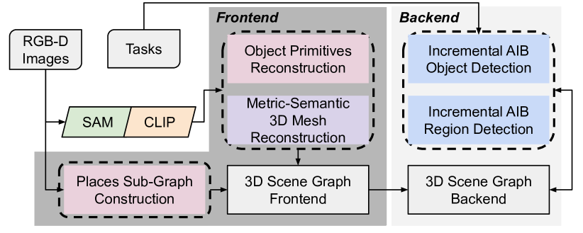
Figure 3: Clio’s frontend takes in RGB-D sensor data and constructs the graph of object primitives, the graph of places, and the metric-semantic 3D mesh of the background. Clio’s backend performs Incremental Agglomerative IB to cluster objects and regions based on a user-specified list of tasks.

V-B Clio Backend

After the frontend populates the background mesh, object primitives, and places, the backend performs clustering to extract and retain task-relevant objects and regions.

Task-Driven Object Detection. Clio runs our Agglomerative IB method on the over-segmented 3D object primitives from the frontend. As input to IB, we construct a graph where the nodes are the object primitives and add edges between nodes if the corresponding primitives have 3D bounding boxes with non-zero overlap. We compute $p({y}|{x})$ as described in eq. (5). In this case, the null task can be thought of as background task-irrelevant objects. We set $\alpha=0.23$. We provide two versions of Clio. The first, Clio-batch assumes all primitives for the entire scene have first been generated and then clusters all objects segments using eq. (3). The second, Clio-online takes in a real-time stream of images and constructs a map using our incremental IB algorithm, where clustering is only performed again for the connected components affected by the most recent measurements.

Task-Driven Clustering of Places. Clio finally performs Agglomerative IB at every backend update to cluster the place nodes into regions. The task-driven clustering is applied to the graph of places produced by Hydra [7], where each place node in the graph is a primitive for IB and each edge in the place graph is considered as a putative merge for clustering. We compute $p({y}|{x})$ between the tasks and place nodes in the same manner as the objects. Each resulting cluster of place nodes is used to create a new region. Two regions share an edge if any places in the two regions also share an edge.

VI Experiments

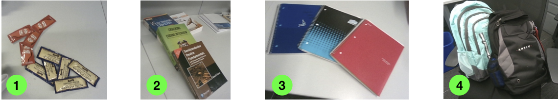
(a) Sample of four regions of the Cubicle dataset

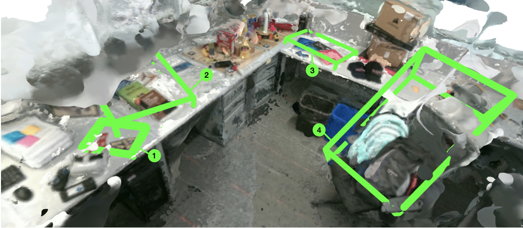
(b) Clio clustering results shown for the following tasks: (1) get condiments packets, (2) get textbooks, (3) get notebooks, (4) clean backpacks.

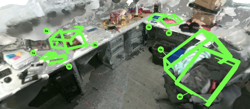
(c) Clio clustering results shown for the following tasks: (1a) get hot sauce packets, (1b) get grey poupon packets, (2a) read Cracking the Coding Interview book, (2b) read brown textbook, (3a) pack blue notebooks, (3b) pack red notebook, (4a) get teal backpack, (4b) clean black backpack.

Figure 4: Examples of portions of the Cubicle dataset that require a task to provide rectification of how an object should be defined. The figure showcases Clio’s clustering results for two sets of tasks, listed under (b) and (c); 14 additional tasks identical for both tests are included in the task list during clustering but not shown for clarity.

Our experiments show that Clio (i) constructs more parsimonious and useful map representations (Section VI-A), (ii) performs on par with the state of the art in closed-set settings where the task is implicitly specified by a closed dictionary (Section VI-B), (iii) is able to cluster the environment into meaningful semantic regions (Section VI-C), and (iv) can support task execution on real robots (SectionVI-D).

VI-A Open-Set Object Clustering Evaluation

Experimental Setup. To test Clio in realistic and diverse scenes, we collect four datasets, in an office, an apartment, a cubicle, and a large-scale university building, which covers five floors including a machine shop, classroom, lounge, meeting rooms, to cluttered workspaces, and an aircraft hangar. For the Office, Apartment, and Cubicle datasets we manually annotate ground truth 3D bounding boxes for objects associated to the given set of tasks. For evaluation purposes, tasks are chosen such that there is an unambiguous set of objects best suited for the tasks, to reduce subjective reasoning over what constitutes a ground truth set of objects. A complete list of tasks is provided in Appendices -D--F.

Metrics. For this evaluation, after constructing the 3D scene graph, we query the $n$ best objects for every task — where $n$ is the number of ground truth labels of objects relevant for the task. We then compare the IOU of the 3D bounding boxes of the detected objects to the ground truth objects. We additionally report two measures of accuracy: strict accuracy (SAcc), which is the fraction of times the bounding box of an estimated object contains the centroid of the ground truth bounding box, and the bounding box of the ground truth object contains the centroid of the estimated bounding box, and relaxed accuracy (RAcc), which is the fraction of cases where at least one of the two prior conditions is met. We also measure strict and relaxed precision as the total number of strict and relaxed true detections divided by the total number of detections that have at least 90% cosine similarity score to a task as the most similar object. The F1 score is computed as the harmonic mean of the relaxed accuracy and relaxed precision. We also include the average runtime per frame (tpf) to build the scene graph and total number of objects in the final scene graph.

Compared Techniques. As our queries do not include negation or multi-step affordances, we run ConceptGraphs with only CLIP in place of LLava+GPT, as CLIP was shown to have similar performance for these types of queries in [9]. In addition to running ConceptGraphs and Clio, we also test: Khronos, which performs clustering as described in [62] with parameters $\theta_{\text{track}}=0.7$, $\gamma=0.4$, $\theta_{\text{vol}}=8.0$, and $\theta_{\text{obs}}=3$, and Clio-Prim, which only computes the set of input 3D object primitives to Clio with parameters $\theta_{\text{track}}=0.9$, $\gamma=0.6$, $\theta_{\text{vol}}=8.0$, and $\theta_{\text{obs}}=2$; essentially, Clio-Prim is the output of the Clio frontend, hence this comparison allows assessing the effectiveness of the IB clustering in Clio. To show the importance of being task-driven, we further include task-aware versions of the baselines: Khronos-task and ConceptGraphs-task take the results of Khronos and ConceptGraphs and remove mapped objects that do not have a high enough ($\alpha=0.23$) cosine similarity to at least one task in the provided task list. We include results for both Clio-batch, which takes in all primitives of a scene and is executed only once at the end of the mapping session, and Clio-online, which incrementally receives primitives for real-time mapping. We use CLIP model ViT-L/14 and generate results with an RTX 3090 GPU and Intel i9-1290K CPU. Results are shown in Table I. Results for OpenCLIP model ViT-H-14 are included in Section -H.

Scene	Method	IOU$\uparrow$	SAcc$\uparrow$	RAcc$\uparrow$	Sprec$\uparrow$	Rprec$\uparrow$	F1$\uparrow$	Objs$\downarrow$	TPF(s)$\downarrow$
	CG [9]	0.06	0.44	0.61	0.17	0.28	0.39	181	2.0
	Khronos [62]	0.17	0.78	0.83	0.12	0.11	0.20	628	0.31
	Clio-Prim	0.18	0.72	0.72	0.09	0.10	0.17	1070	0.28
	CG-task	0.06	0.44	0.61	0.38	0.50	0.55	26	2.0
	Khronos-task	0.17	0.78	0.83	0.14	0.14	0.24	133	0.31
	Clio-batch	0.17	0.83	1.0	0.33	0.40	0.57	48	0.31∗
	Clio-online	0.22	0.89	0.89	0.48	0.48	0.63	92	0.30
Cubicle	CG [9]	0.07	0.26	0.52	0.09	0.16	0.25	751	8.1
	Khronos [62]	0.17	0.70	0.70	0.30	0.30	0.42	1202	0.31
	Clio-Prim	0.19	0.74	0.78	0.20	0.20	0.32	1880	0.27
	CG-task	0.05	0.19	0.41	0.36	0.64	0.50	35	8.1
	Khronos-task	0.13	0.56	0.56	0.34	0.34	0.42	140	0.31
	Clio-batch	0.13	0.67	0.82	0.64	0.79	0.80	84	0.30∗
	Clio-online	0.11	0.56	0.59	0.63	0.67	0.63	131	0.29
Office	CG [9]	0.07	0.38	0.62	0.17	0.25	0.35	339	2.2
	Khronos [62]	0.11	0.45	0.76	0.08	0.12	0.21	1093	0.26
	Clio-Prim	0.12	0.35	0.59	0.07	0.09	0.16	1694	0.20
	CG-task	0.03	0.21	0.35	0.30	0.45	0.39	21	2.2
	Khronos-task	0.11	0.41	0.72	0.15	0.21	0.32	162	0.26
	Clio-batch	0.11	0.52	0.72	0.34	0.45	0.55	90	0.23∗
	Clio-online	0.07	0.35	0.52	0.31	0.42	0.46	99	0.26
Apartment

TABLE I: Results of locating objects of interest via open-set task query for three datasets. We include results for CLIP ViT-L/14. The Office, Apartment, and Cubicle datasets have 27, 28, and 18 objects of interest respectively. Results generated with 3090 GPU and Intel i9-12900K. Shaded methods are informed by the list of tasks. First and second-best results are bolded and underlined, respectively. ^∗Total time for Clio-batch normalized by number of images; clustering step for batch run once on entire graph takes approximately 30 seconds and thus not suitable for online use.

Results. First of all, we observe that task-informed approaches (shaded blue rows in Table I) generally lead to better performance metrics while retaining a much smaller amount of objects (“Objs” column); this validates our claim that metric-semantic mapping needs to be task-driven. In particular, in some cases Clio retains an order of magnitude less objects compared to task-agnostic baselines (cf. with the number of objects in Clio-Prim, which is essentially Clio without the Information Bottleneck task-driven clustering). Second, we observe that Clio largely outperforms baselines across datasets, with Clio-batch and Clio-online ranking first or second in all but 2 cases, namely, the IOU and SAcc metric in the Office dataset. Many of the objects in the Office dataset (e.g., staplers, bike helmet) are typically detected as isolated primitives, hence we see that the knowledge of the task has a lesser impact on this dataset, while still improving performance across all other metrics. Third, we observe that Clio is able to run in a fraction of a second and is around 6 times faster than ConceptGraphs; Khronos and Clio-Prim also run in real-time, but have sub-par performance in terms of other metrics. Finally, Clio-batch and Clio-online have similar performance in most cases. Their performance difference is due to the fact that Clio-online is executed in real-time and might drop frames as required to keep up with the camera image stream. This difference sometimes helps and sometimes hinders the performance metrics.

As an example of Clio’s ability to use task information to form adequate scene representations, Fig. 4 shows a subset of the detected objects from Clio for two different tasks sets. For a task involving getting all condiment packets, Clio represents a group of different type condiment packets collectively as one object, while for an alternative set of tasks requiring specific types of condiments, Clio represents the pile as multiple objects distinguished by sauce type, yielding a more flexible and useful scene representation. Qualitative results for the large-scale five-floor building dataset are included in the video attachment.

VI-B Closed-Set Object Evaluation

While Clio is designed for open-set detection, we include results on the closed-set Replica [17] dataset using the evaluation method performed by [8, 9] to show that our task-aware mapping formulation does not degrade performance on closed-set mapping tasks. Here, our list of tasks is the set of object labels present in each Replica scene where each label is changed to be “an image of {class}” following [9]. For both Clio and [9], after creating the scene graph, we assign the label with the highest cosine similarity to each of the detected objects. To improve the reliability of CLIP given the low texture regions of the Replica dataset, we include global context CLIP vectors by incorporating dense CLIP features from [63] for Clio. We report accuracy as the class-mean recall (mAcc) and the frequency-weighted mean intersection-over-union (f-mIOU). Table II shows that Clio achieves comparable performance to the leading zero-shot methods, indicating that our task-aware clustering does not degrade performance on closed-set tasks.

Method	mAcc	F-mIOU
MaskCLIP	4.53	0.94
Mask3former + Global CLIP feat	10.42	13.11
ConceptFusion	24.16	31.31
ConceptFusion + SAM	31.53	38.70
ConceptGraphs	40.63	35.95
ConceptGraphs-Detector	38.72	35.82
Clio-batch	37.95	36.98

TABLE II: Closed-set semantic segmentation experiments on 8 scenes from the Replica [17] dataset. Baseline results reported from [9].

VI-C Open Vocabulary Places Clustering

Since manually labeling semantic 3D regions is a highly subjective task, we evaluate the performance of Clio’s regions via a proxy closed-set task, where Clio is provided the set of possible room labels for the scenes as tasks. We label rooms in three datasets: Office, Apartment, and Building. We do not analyze the Cubicle or Replica [17] as they only consists of a single room. We set $\alpha=0$ to disable assignment to the null task as every place is relevant to at least one room label, and we hold all parameters constant across scenes.

Dataset	Method	Precision$\uparrow$	Recall$\uparrow$	F1$\uparrow$
Apartment	Hydra	0.93 $\pm$ 0.01	0.87 $\pm$ 0.01	0.90 $\pm$ 0.00
	Clio (closest)	0.87 $\pm$ 0.06	0.78 $\pm$ 0.02	0.82 $\pm$ 0.01
	Clio (average)	0.98 $\pm$ 0.02	0.54 $\pm$ 0.00	0.69 $\pm$ 0.00
Office	Hydra	0.61 $\pm$ 0.03	0.84 $\pm$ 0.03	0.70 $\pm$ 0.01
	Clio (closest)	0.67 $\pm$ 0.03	0.79 $\pm$ 0.01	0.72 $\pm$ 0.01
	Clio (average)	0.73 $\pm$ 0.01	0.80 $\pm$ 0.00	0.76 $\pm$ 0.01
Building	Hydra	0.87 $\pm$ 0.01	0.71 $\pm$ 0.02	0.78 $\pm$ 0.01
	Clio (closest)	0.72 $\pm$ 0.04	0.82 $\pm$ 0.01	0.77 $\pm$ 0.02
	Clio (average)	0.79 $\pm$ 0.02	0.84 $\pm$ 0.01	0.81 $\pm$ 0.01

TABLE III: Comparison of geometric room segmentation accuracy.

We use the precision and recall metrics presented by [7] to compare our proposed CLIP embedding vector association strategy, Clio (average), as well another more naive strategy, Clio (closest), which uses the embedding vector taken from the closest image that the place node is still visible from. In addition, we use the purely geometric room segmentation approach from Hydra [7] as a point of comparison for the closed set performance. Results from this comparison are presented in Table III, which also includes the F1 score as a summary statistic. The results in Table III are averaged over 5 trials, and standard deviation of all metrics is reported. We note that our chosen association strategy outperforms both the purely geometric approach of Hydra [7] and the more naive Clio (closest) for the Office and Building scene, but performs relatively poorly in terms of F1 score in the Apartment. This is due to the nature of the scenes; the Office and the Building scene contain labeled open floor-plan rooms that require semantic knowledge to be detected (e.g., a kitchenette in the Office scene or stairwells in the Building scene). The Apartment primarily contains geometrically distinct rooms, which are straightforward to segment with the geometric approach in [7], and are instead over-segmented by Clio, as evident from the high precision but low recall of our method. On the other hand, semantically similar regions that are connected, as present in the Office, lead to under-segmentation and lower recall compared to Hydra [7].

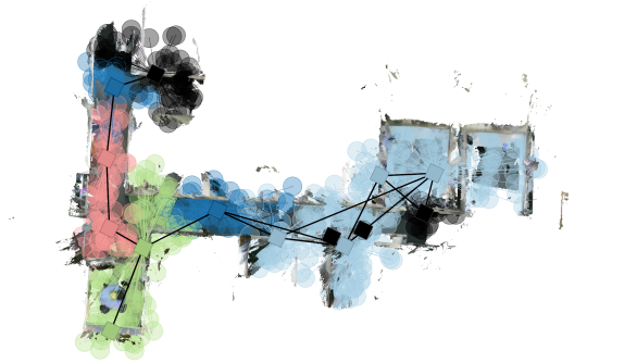
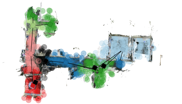
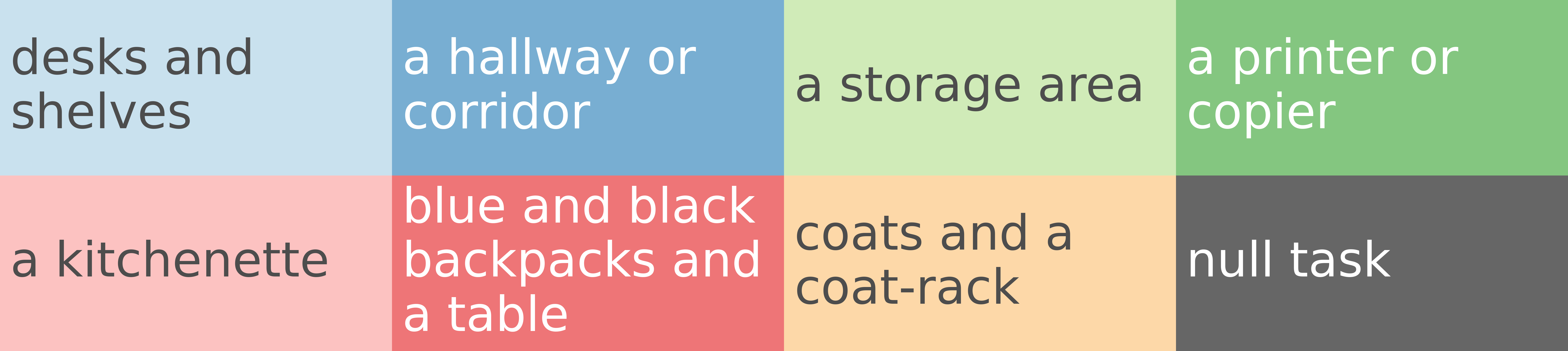
Figure 5: Qualitative examples of places clustering. The first figure shows regions that result from clustering by task prompts resembling room category labels. The second figure shows regions that result from clustering by task prompts that are a mix of potential rooms and objects.

Fig. 5 qualitatively demonstrates Clio’s capability to produce task-relevant regions on the Office scene. We compare two different granularities of tasks; the first is similar to the provided room labels in the closed-set proxy evaluation while the second is much more granular and object-driven. The resulting regions reflect this difference in granularity despite being produced by Clio using the same set of parameters. More visualizations supporting the meaningfulness of Clio’s region clustering are provided in Section -J.

VI-D Online Evaluation on Spot

To demonstrate the real-time use of Clio for robotics, we conduct mobile manipulation experiments using a Boston Dynamics Spot quadruped robot equipped with an arm and gripper. During the experiments, the robot constructs a map with Clio in real-time while exploring a scene, and then is tasked to navigate to and pick up objects matching a provided natural language prompt (e.g., Fig. 2). We use the onboard front-left and front-right RGB-D cameras and odometry from Spot as inputs to Clio. We run Clio on a laptop capable of being mounted on the robot that is equipped with an Intel i9-13950HX CPU with $24$ cores, $64$GB of RAM, and an NVIDIA GeForce RTX $4090$ Laptop GPU.

For these experiments, a separate process (running in parallel to Clio) allows the user to input a natural language command to pickup or drop-off an object. The command is embedded using CLIP and used to select the object in the scene graph with the highest cosine similarity to the prompt. Then we compute the shortest path through the place nodes to the target object via Dijkstra’s algorithm. We smooth and follow the resulting trajectory to navigate to the object by commanding Spot to sequentially navigate to sampled waypoints. After reaching the target object, we select the pixel centroid from the current input semantic segments with the highest cosine similarity to the prompt embedding as a grasp candidate as input to the Spot API grasp command.

We perform 7 trials of a mobile manipulation experiment where we use Clio and our planner described above to grasp a variety of objects. Each trial consists of a mapping phase, where we teleoperate Spot to observe all the objects in the scene (consisting of two room-like areas joined by a hallway). After the mapping phase, we move Spot to a starting location and then command grasps of 3 random target objects for a total of 21 unique grasp attempts. Clio runs the entire time during the trial, and no post-processing of the 3D scene graph is performed. We present a breakdown of the 21 trials in Fig. 6. Overall, we achieve a 57% success rate for the grasps and a 71% success rate if we disregard the cases where Spot failed to actually grasp a correctly identified object. Notably, Clio was only unable to select the correct target object in the scene graph once (i.e., the “Wrong Object” failure category). The video attachment also demonstrates a pick-and-place experiment with a sequence of 4 pick-and-place actions over a larger area where Spot is operated with the laptop onboard. These experiments together emphasize the suitability of Clio for use onboard real robotic platforms.

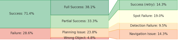
Figure 6: Breakdown of grasp results for the 21 object grasp attempts performed by Spot. “Wrong object” refers to the wrong Clio object being selected, “Detection failure” refers to the selected image coordinates for grasping not corresponding to the target object, “Navigation issue” refers to the trajectory resulting in a pose where the object was not visible, “Spot Failure” refers to the Spot API failing to pick up a correctly identified grasp, and “Success (retry)” refers to the Spot API grasp command failing to pick up the object on the first attempt but succeeding after repeated attempts.

VII Limitations

Despite the encouraging experimental results, our approach has multiple limitations. First, while our method is zero-shot and is not bound to any particular foundation model, it does inherit some limitations from the foundation models used in implementation such as strong vulnerability to prompt tuning. For instance, in Section -H, we discuss how performance is affected by different CLIP models. Second, we currently average CLIP vectors when merging two primitives, but it would be interesting to consider more grounded ways to combine their semantic descriptions. Third, Clio can over-cluster if two primitives individually have similar cosine similarity to the same task but somehow the task requires distinguishing them as separate objects (e.g., we might want to distinguish a fork from a knife when setting the table, even though they might have similar relevance to the task). Finally, we currently consider relatively simple, single-step tasks. However, it would be desirable to extend the proposed framework to work with a set of high-level, complex tasks.

VIII Conclusion

We have presented a task-driven formulation for 3D metric-semantic mapping, where a robot is provided with a list of natural language tasks and has to create a map whose granularity and structure is sufficient to support those tasks. We have shown that this problem can be expressed in terms of the classical Information Bottleneck and have developed an incremental version of the Agglomerative Information Bottleneck algorithm as a solution strategy. We have integrated the resulting algorithm in a real-time system, Clio, that constructs a 3D scene graph —including task-relevant objects and regions— as the robot explores the environment. We have also demonstrated Clio’s relevance for robotics, by showing it can be executed in real-time onboard a Spot robot and support pick-and-place mobile manipulation tasks.

-A Agglomerative Information Bottleneck

Algorithm 1 provides the pseudocode for the Agglomerative Information Bottleneck [14] discussed in Section IV. The goal of Algorithm 1 is to find an optimal hard clustering assignment $p(\tilde{x}|x)$ that compresses an initial signal $X$ into a compressed signal $\tilde{X}$ while preserving relevant information about a relevancy variable $Y$ (which in our case is a set of tasks). The algorithm runs until a set threshold $\bar{\delta}$ is reached which is used to regulate the amount of compression with respect to preserving information about $Y$.

Algorithm 1 Agglomerative Information Bottleneck

0:  $\bar{\delta}$, initial primitives $\{x_{1},\ldots x_{N}\}=X$, task-list $Y$

0:  $p(\tilde{x}|x)$: hard assignment of primitives to clusters % Initialization:

1:  set $p(y|x)$ using $eq.~{}\eqref{eq:pyx}$

2:  $\tilde{x}_{i}=x_{i}\ \forall x_{i}\in X$

3:  $p(\tilde{x}_{i})=p(x_{i})=1/N$ % uniform distribution

4:  $p(y|\tilde{x})=p(y|x_{i}),\forall y\in Y$

5:  Compute $d_{ij}$ using eq. (2) for all $i=1,\ldots,|X|$ and $j=1,\ldots,|Y|$ % Main loop:

6:  while $\delta<\bar{\delta}$ do

7:     $d_{ab}=\min_{ij}(d_{ij})$

8:     $p(\tilde{x})=p(x_{a})+p(x_{b})$

9:     $p(y|\tilde{x})=\frac{p(x_{a},y)+p(x_{b},y)}{p(\tilde{x})}\ \forall y\in Y$

10:     $p(\tilde{x}|x)=1\ if\ x\in\tilde{x}_{a}\cup\tilde{x}_{b},\ 0\ \text{ otherwise }\ \forall x\in X$

11:     compute $\delta$ from eq. (3) for batch or eq. (6) for online

12:  end while

13:  return  $p(\tilde{x}|x)$

-B Incremental Agglomerative IB

As mentioned in Section IV, we form an incremental version of the Agglomerative IB to run Clio online. For this, we run Agglomerative IB on each individual connected component $c$ using a re-weighted definition of $\delta(k)$. Assuming that $p(x)$ is a uniform distribution we can write the incremental equivalent of $\delta(k)$ as:

$$\delta_{c}(k)=\frac{|X_{c}|}{|X|}\frac{I((\tilde{X_{c}})_{k};Y)-I((\tilde{X_{c}})_{k-1};Y)}{I(X;Y)}$$ (6)

where $X_{c}$ are the primitives in component $c$. This gives the exact same result as Agglomerative IB on the full graph which lets us implement the stopping condition of Algorithm 1 across each connected component Therefore, we can solve Agglomerative IB in an incremental manner by only performing Agglomerative IB on the subset of connected components of the graph that are affected by new measurements using Algorithm 2. Here, when Clio receives new primitives $X_{new}$, we add the primitives to their respective sub-graphs and for each of the sub-graphs that received new primitives we run Agglomerative IB until the stopping condition from eq. (6) is met, repeating as new primitives are received.

Algorithm 2 Incremental Agglomerative Information Bottleneck

0:  $c\in{\cal C}$ {set of connected sub-graphs}    $X_{new}$ {newly received primitives}

0:  $p(\tilde{x}|x)$: hard assignment of primitives to clusters

1:  ${\cal C}\leftarrow X_{new}$ {update corresponding sub-graphs with new primitives}

2:  for each $c$ in ${\cal C}$ do

3:     if $c$ updated then

4:        update $p(\tilde{x}|x),x\in X_{c},\ \tilde{x}\in\tilde{X}_{c}$ with Algorithm 1 using stop condition from eq. (6)

5:     end if

6:  end for

7:  return  $p(\tilde{x}|x)$

Here we provide the proof to the expression in eq. (6). Given a connected component $c$ we want to cluster $X_{c}$, the primitives within the component, into clusters $\tilde{X_{c}}$ independent of the rest of the graph. Let us also define $o$ for the primitives not in $c$ such that $X_{c}\cup X_{o}=X$ and $X_{c}\cap X_{o}=\varnothing$. Since $P(X)$ is uniformly distributed,

$$I(X_{c};Y)=\frac{1}{|X_{c}|}\sum_{X_{c}}p(y|x)\log(\frac{p(y|x)}{p(y)})$$ (7)

Let us define $\Delta$ such that

$$\Delta=\frac{1}{|X|}\sum_{X_{o}}p(y|x)\log(\frac{p(y|x)}{p(y)})$$ (8)

this allows us to rewrite $I(X;Y)$ as follows:

$$I(X;Y)= \frac{1}{|X|}\sum_{X_{c}}p(y|x)\log(\frac{p(y|x)}{p(y)})+\Delta$$ (9)

$$= \frac{|X_{c}|}{|X|}I(X_{c};Y)+\Delta$$

since we are only clustering in $c$,

$$I(\tilde{X}_{k};Y)=\frac{|X_{c}|}{|X|}I((\tilde{X}_{c})_{k};Y)+\Delta$$ (10)

Substituting in for $I(\tilde{X}_{k};Y)$ and $I(\tilde{X}_{k-1};Y)$ in (3), we obtain our re-weighted expression in (6).

-C Office, Apartment, and Cubicle Datasets

For each of the office, apartment, cubicle and building datasets, we collect RGB-D images with an Intel RealSense D455. A visualization of the scenes are shown in Fig. 7.

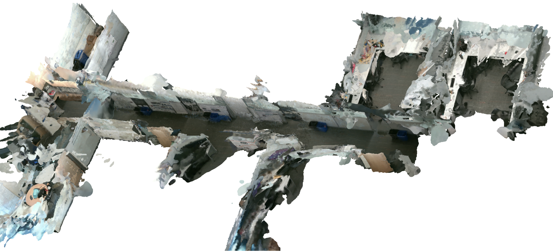
(a) Office Scene

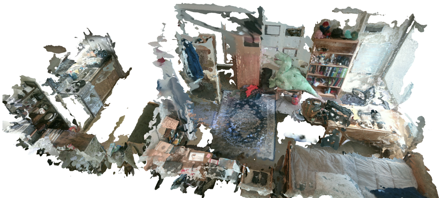
(b) Apartment Scene

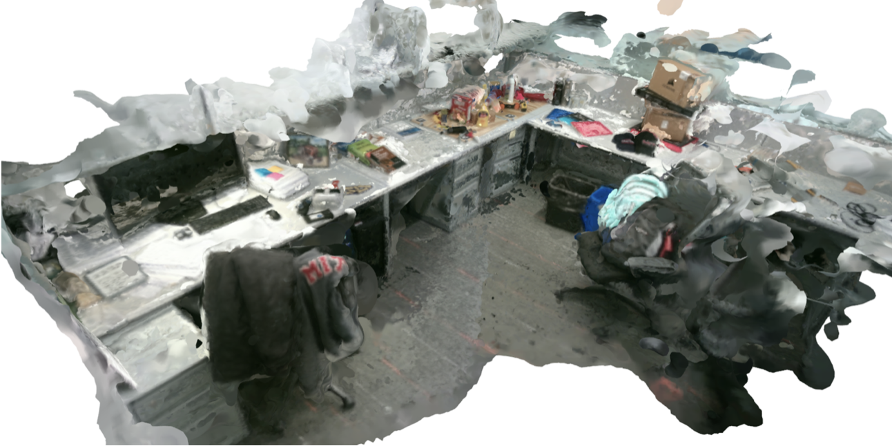
(c) Cubicle Scene

Figure 7: Custom open-vocabulary 3D datasets of an office floor, apartment, and cubicle.

A visualization of the resulting scene graphs are also shown in Fig. 8.

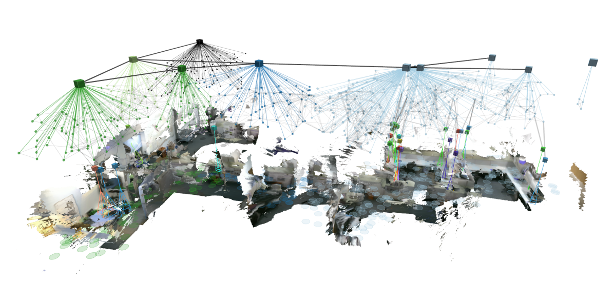
(a) Office Scene

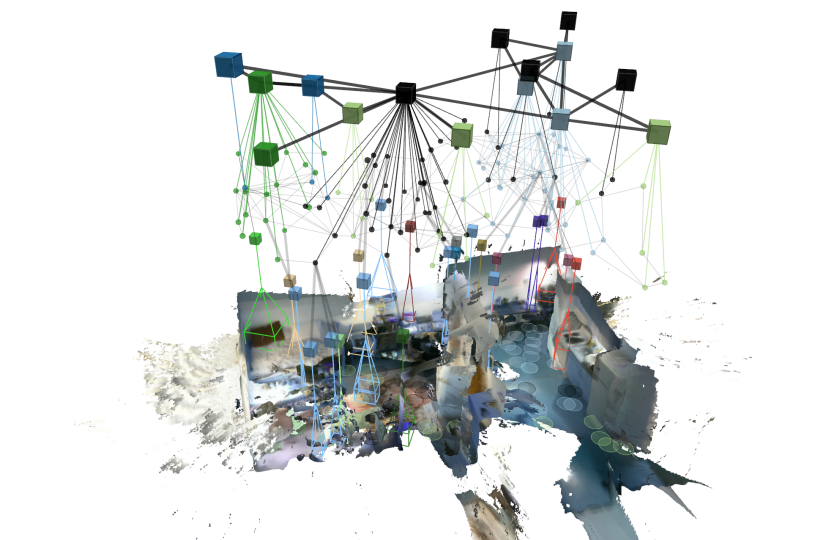
(b) Apartment Scene

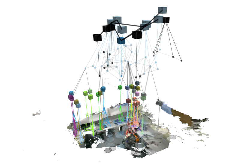
(c) Cubicle Scene

Figure 8: Example 3D scene graphs for the self-collected Office, Apartment and Cubicle datasets. Scene graphs layers are drawn in the following order: objects (as cubes), places (as spheres) and regions (as cubes). The bounding box of each object is drawn below, and a footprint is drawn for each place primitive to highlight the 2D positions of the nodes. Places and regions are colored by their closest task as shown in the legend below each figure.

-D Office Scene Task List

Here we provide a list of tasks used during mapping and querying of the office scene. The number of objects assigned to each task is included in parentheses. There are 27 distinct objects in total.

1. get a black Expo marker (2)

2. get a painting of a tractor (1)

3. move rack of magazines (1)

4. get my Signals and Systems textbook (1)

5. something to cut paper (3)

6. get black glasses (1)

7. get box of tissues (2)

8. get my gloves (1)

9. get orange knit hat to keep my head warm (1)

10. get rock with holes (1)

11. something to put on a hot dog (1)

12. get can of tuna (1)

13. grab black backpack (1)

14. grab teal backpack (1)

15. move the bin of clothes (1)

16. move the printer (3)

17. organize the pile of red dishes and plates (1)

18. get stapler (2)

19. get a yellow rubber duck (1)

20. organize the pile of hardware tools (1)

-E Apartment Scene Task List

Here we provide a list of tasks used during mapping and querying of the apartment scene. The number of objects assigned to each task is included in parentheses. There are 28 distinct objects in total.

1. get can of WD-40 (1)

2. clean toaster (1)

3. find deck of cards (1)

4. find pile of hats (1)

5. find spice bottles (1)

6. get a kitchen knife (3)

7. get pocket knife (1)

8. get bike helmet (1)

9. get bottle of tide (1)

10. get cast iron skillet (1)

11. get hair dryer (1)

12. get hairbrush (1)

13. get notebooks binders (1)

14. get pizza cutting wheel (1)

15. get soy sauce (1)

16. get toolbox (1)

17. get violin case (1)

18. move pile of clothes (1)

19. move rack of dishes (1)

20. bring me a pillow (2)

21. get alarm clock (1)

22. get all chocolate snacks (1)

23. get chapstick (1)

24. get first aid kit (1)

25. move popcorn bags (1)

-F Cubicle Scene Task List

Here we provide a list of tasks used during mapping and querying of the cubicle scene. All tasks here have one corresponding object. There are 18 objects in total.

1. get condiment packets

2. get drink cans

3. get eyeglasses

4. get glasses case

5. get grey jacket

6. get my silver water bottle

7. get notebooks

8. get mudstone rock

9. tool to cut paper

10. get sticky notes

11. get textbooks

12. get waste bins

13. move hats

14. clean backpacks

15. get red crockery

16. get hardware drill

17. get quartz rock

18. get tape measure

-G Building Scene Task List

Here we provide a list of tasks used during mapping and querying of the building scene. Note that some tasks have many occurrences of relevant items in the dataset.

1. get Lysol

2. get vacuum cleaner

3. get fire extinguisher

4. get yellow wet floor sign

5. get clamps

6. get epoxy and resin bottles

7. get roles of tape

8. locate screwdrivers

9. move jet engine

10. get earmuffs

11. move co2 tanks

12. check office printer

13. get books

14. get basketball

15. refill dish soap bottles

16. get trashbins

17. move pink foam

18. stack blue foam

19. check microwave

20. clean sink

21. get bottles of cleaner

22. stuff with MIT on it

23. get tape measure

24. grab airplane wing

25. clean stairs

-H Open Vocabulary Tasks on OpenCLIP model

Here we repeat the experiments from Table I but this time use a different CLIP model (ViT-H-14 from OpenCLIP [64]). Due to the higher compute requirements for this model we do not run Clio-online and instead only run Clio-batch. We found that this model tends to produce higher cosine similarity scores between image primitives and tasks for both relevant and irrelevant pairings, and thus we increase the null task value and cosine similarity threshold ($\alpha$) to 0.26 for Clio, Khronos-task, and ConceptGraphs-task.

Scene	Method	IOU$\uparrow$	SAcc$\uparrow$	RAcc$\uparrow$	Sprec$\uparrow$	Rprec$\uparrow$	F1$\uparrow$	Objs$\downarrow$	TPF(s)$\downarrow$
	CG [9]	0.06	0.56	0.89	0.39	0.52	0.65	231	3.15
	Khronos [62]	0.18	0.83	0.83	0.16	0.17	0.28	623	1.16
	Clio-Prim	0.20	0.72	0.89	0.15	0.15	0.25	956	1.14
	CG-thres	0.06	0.56	0.89	0.43	0.57	0.70	49	3.15
	Khronos-thres	0.18	0.83	0.83	0.19	0.20	0.32	195	1.16
	Clio-batch	0.17	0.78	0.94	0.28	0.31	0.47	96	1.16∗
cubicle	CG [9]	0.08	0.35	0.59	0.23	0.30	0.40	434	12.33
	Khronos [62]	0.15	0.63	0.63	0.23	0.23	0.34	1202	1.15
	Clio-Prim	0.16	0.63	0.63	0.20	0.21	0.31	1717	1.13
	CG-thres	0.07	0.26	0.52	0.16	0.25	0.34	257	12.33
	Khronos-thres	0.14	0.59	0.59	0.24	0.24	0.34	334	1.15
	Clio-batch	0.11	0.59	0.78	0.35	0.45	0.57	213	1.15∗
office	CG [9]	0.08	0.30	0.52	0.13	0.20	0.29	908	3.54
	Khronos [62]	0.09	0.35	0.59	0.11	0.16	0.25	1081	1.03
	Clio-Prim	0.13	0.48	0.69	0.12	0.16	0.26	1482	0.99
	CG-thres	0.06	0.31	0.55	0.39	0.55	0.55	68	3.54
	Khronos-thres	0.09	0.35	0.59	0.11	0.17	0.26	363	1.03
	Clio-batch	0.10	0.38	0.69	0.16	0.28	0.40	222	1.01∗
apartment

TABLE IV: Results of locating objects of interest via open-set task query for three datasets. We include results for OpenCLIP ViT-H-14. The office, apartment, and cubicle datasets have 27, 28, and 18 objects of interest respectively. Results generated with 3090 GPU and Intel i9-12900K. Shaded methods are informed by the list of tasks. First and second-best results are bolded and underlined, respectively. ^∗Total time for Clio-batch normalized by number of images; clustering step for batch run once on entire graph takes approximately 30 seconds and thus not suitable for online use.

-I Closed-Set Places Clustering Task List

For the experiment shown in Table III, we report the task prompts used for each scene. Note that we prefix each categorical prompt with “an image of …” to mimic similiar closed-set experiments (e.g., Replica).

For the Apartment scene, we used

1. an image of a kitchen

2. an image of a bedroom

3. an image of a doorway

For the Office scene, we used

1. an image of a computing workspace

2. an image of a hallway or corridor

3. an image of a kitchenette

4. an image of a conference room

For the Building scene, we used

1. an image of a student lounge

2. an image of a kitchnette or utility closet

3. an image of a classroom

4. an image of a conference room

5. an image of a stairway

6. an image of a workshop or machine shop

7. an image of an aircraft hangar of garage

-J Places Clustering Results Visualization

We include an additional visualization of clustering places into relevant regions on the office dataset by showing example figures of a subset of the regions in Fig. 9 to supporting the meaningfulness of Clio’s region clustering.

Figure 9: Visualization of region clustering results on office dataset with example images from regions included for two different task lists.

References

- [1] S. Soatto and A. Chiuso, “Visual representations: Defining properties and deep approximations,” in Intl. Conf. on Learning Representations (ICLR), 2016.
- [2] C. Cadena et al., “Past, present, and future of simultaneous localization and mapping: Toward the robust-perception age,” IEEE Trans. Robotics, vol. 32, no. 6, pp. 1309–1332, 2016, arxiv preprint: 1606.05830, (pdf).
- [3] I. Armeni, Z. He, J. Gwak, A. Zamir, M. Fischer, J. Malik, and S. Savarese, “3D scene graph: A structure for unified semantics, 3D space, and camera,” in Intl. Conf. on Computer Vision (ICCV), 2019, pp. 5664–5673.
- [4] A. Rosinol, A. Gupta, M. Abate, J. Shi, and L. Carlone, “3D dynamic scene graphs: Actionable spatial perception with places, objects, and humans,” in Robotics: Science and Systems (RSS), 2020, (pdf), (media), (video). [Online]. Available: http://news.mit.edu/2020/robots-spatial-perception-0715
- [5] S. Wu, J. Wald, K. Tateno, N. Navab, and F. Tombari, “SceneGraphFusion: Incremental 3D scene graph prediction from RGB-D sequences,” in IEEE Conf. on Computer Vision and Pattern Recognition (CVPR), 2021.
- [6] N. Hughes, Y. Chang, and L. Carlone, “Hydra: a real-time spatial perception engine for 3D scene graph construction and optimization,” in Robotics: Science and Systems (RSS), 2022, (pdf).
- [7] N. Hughes, Y. Chang, S. Hu, R. Talak, R. Abdulhai, J. Strader, and L. Carlone, “Foundations of spatial perception for robotics: Hierarchical representations and real-time systems,” Intl. J. of Robotics Research, 2024, arXiv preprint: 2305.07154, (pdf),(video).
- [8] K. Jatavallabhula et al., “Conceptfusion: Open-set multimodal 3d mapping,” in Robotics: Science and Systems (RSS), 2023.
- [9] Q. Gu et al., “Conceptgraphs: Open-vocabulary 3d scene graphs for perception and planning,” 2023.
- [10] A. Kirillov et al., “Segment anything,” arXiv:2304.02643, 2023.
- [11] A. Radford et al., “Learning transferable visual models from natural language supervision,” in Intl. Conf. on Machine Learning (ICML), ser. Proceedings of Machine Learning Research, M. Meila and T. Zhang, Eds., vol. 139. PMLR, 18–24 Jul 2021, pp. 8748–8763.
- [12] A. M. Treisman and G. Gelade, “A feature-integration theory of attention,” in Cognitive Psychology, vol. 12, 1980, pp. 97–136.
- [13] N. Tishby, F. Pereira, and W. Bialek, “The information bottleneck method,” Proc. of the Allerton Conference on Communication, Control and Computation, vol. 49, 07 2001.
- [14] N. Slonim and N. Tishby, “Agglomerative information bottleneck,” in Advances in Neural Information Processing Systems (NIPS), ser. NIPS’99, 1999, pp. 617–623.
- [15] H. Liu, C. Li, Q. Wu, and Y. J. Lee, “Visual instruction tuning,” in Advances in Neural Information Processing Systems (NIPS), 2023.
- [16] OpenAI, “GPT-4 technical report,” CoRR, vol. abs/2303.08774, 2023. [Online]. Available: https://doi.org/10.48550/arXiv.2303.08774
- [17] J. Straub et al., “The Replica dataset: A digital replica of indoor spaces,” arXiv preprint arXiv:1906.05797, 2019.
- [18] M. Oquab et al., “Dinov2: Learning robust visual features without supervision,” arXiv preprint arXiv:2304.07193, 2023.
- [19] Y. Hong, H. Zhen, P. Chen, S. Zheng, Y. Du, Z. Chen, and C. Gan, “3d-llm: Injecting the 3d world into large language models,” arXiv, 2023.
- [20] C. Zhao, Y. Shen, Z. Chen, M. Ding, and C. Gan, “Textpsg: Panoptic scene graph generation from textual descriptions,” 2023.
- [21] M. Chang et al., “Goat: Go to any thing,” arXiv preprint arXiv:2311.06430, 2023.
- [22] S. Garg, “Robohop: Segment-based topological map representation for open-world visual navigation,” in 2nd Workshop on Language and Robot Learning: Language as Grounding, 2023.
- [23] C. Huang, O. Mees, A. Zeng, and W. Burgard, “Visual language maps for robot navigation,” in IEEE Intl. Conf. on Robotics and Automation (ICRA). IEEE, 2023, pp. 10 608–10 615.
- [24] R. Firoozi et al., “Foundation models in robotics: Applications, challenges, and the future,” 2023.
- [25] L. Bianchi, F. Carrara, N. Messina, C. Gennaro, and F. Falchi, “The devil is in the fine-grained details: Evaluating open-vocabulary object detectors for fine-grained understanding,” 2023.
- [26] M. Yuksekgonul, F. Bianchi, P. Kalluri, D. Jurafsky, and J. Zou, “When and why vision-language models behave like bag-of-words models, and what to do about it?” arXiv preprint arXiv:2210.01936, 2022.
- [27] P. Sharma et al., “A vision check-up for language models,” arXiv preprint arXiv:2401.01862, 2024.
- [28] S. Tong, Z. Liu, Y. Zhai, Y. Ma, Y. LeCun, and S. Xie, “Eyes wide shut? exploring the visual shortcomings of multimodal llms,” arXiv preprint: 2401.06209, 2024.
- [29] X. Zhao et al., “Fast segment anything,” 2023.
- [30] K. Kim, Y. Oh, and J. C. Ye, “Zegot: Zero-shot segmentation through optimal transport of text prompts,” 2023.
- [31] Z. Zhou, Y. Lei, B. Zhang, L. Liu, and Y. Liu, “Zegclip: Towards adapting clip for zero-shot semantic segmentation,” in IEEE Conf. on Computer Vision and Pattern Recognition (CVPR), 2023, pp. 11 175–11 185.
- [32] M. Minderer et al., “Simple open-vocabulary object detection,” in European Conf. on Computer Vision (ECCV). Springer, 2022, pp. 728–755.
- [33] S. Liu et al., “Grounding dino: Marrying dino with grounded pre-training for open-set object detection,” arXiv preprint arXiv:2303.05499, 2023.
- [34] B. Li, K. Q. Weinberger, S. Belongie, V. Koltun, and R. Ranftl, “Language-driven semantic segmentation,” in Intl. Conf. on Learning Representations (ICLR), 2022.
- [35] D. Kim, N. Kim, C. Lan, and S. Kwak, “Shatter and gather: Learning referring image segmentation with text supervision,” in IEEE Conf. on Computer Vision and Pattern Recognition (CVPR), 2023.
- [36] R. Huang et al., “Segment3d: Learning fine-grained class-agnostic 3d segmentation without manual labels,” arXiv preprint arXiv:2312.17232, 2023.
- [37] R. Roberts, D.-N. Ta, J. Straub, and F. Dellaert, “Saliency detection and model-based tracking: a two part vision system for small robot navigation in forested environment,” in Intl. Soc. Opt. Eng. (SPIE), 2012.
- [38] B. Mildenhall, P. P. Srinivasan, M. Tancik, J. T. Barron, R. Ramamoorthi, and R. Ng, “Nerf: Representing scenes as neural radiance fields for view synthesis,” arXiv preprint arXiv:2003.08934, 2020.
- [39] B. Kerbl, G. Kopanas, T. Leimkühler, and G. Drettakis, “3d gaussian splatting for real-time radiance field rendering,” ACM Transactions on Graphics, vol. 42, no. 4, July 2023.
- [40] J. Kerr, C. Kim, K. Goldberg, A. Kanazawa, and M. Tancik, “LERF: Language embedded radiance fields,” in iccv, 2023.
- [41] M. Qin, W. Li, J. Zhou, H. Wang, and H. Pfister, “Langsplat: 3d language gaussian splatting,” arXiv preprint arXiv:2312.16084, 2023.
- [42] K. Blomqvist, F. Milano, J. J. Chung, L. Ott, and R. Siegwart, “Neural implicit vision-language feature fields,” arXiv preprint arXiv:2303.10962, 2023.
- [43] C. M. Kim, M. Wu, J. Kerr, K. Goldberg, M. Tancik, and A. Kanazawa, “Garfield: Group anything with radiance fields,” arXiv preprint arXiv:2401.09419, 2024.
- [44] F. Taioli, F. Cunico, F. Girella, R. Bologna, A. Farinelli, and M. Cristani, “Language-enhanced rnr-map: Querying renderable neural radiance field maps with natural language,” in Intl. Conf. on Computer Vision (ICCV), 2023, pp. 4669–4674.
- [45] S. Peng, K. Genova, C. M. Jiang, A. Tagliasacchi, M. Pollefeys, and T. Funkhouser, “Openscene: 3d scene understanding with open vocabularies,” in IEEE Conf. on Computer Vision and Pattern Recognition (CVPR), 2023.
- [46] H. Ha and S. Song, “Semantic abstraction: Open-world 3d scene understanding from 2d vision-language models,” in Conference on Robot Learning (CoRL), 2022.
- [47] J. Wang, J. J. Tarrio, L. de Agapito, P. F. Alcantarilla, and A. Vakhitov, “Semlaps: Real-time semantic mapping with latent prior networks and quasi-planar segmentation,” IEEE Robotics and Automation Letters, vol. 8, pp. 7954–7961, 2023.
- [48] S. Koch, P. Hermosilla, N. Vaskevicius, M. Colosi, and T. Ropinski, “Lang3DSG: Language-based contrastive pre-training for 3D Scene Graph prediction,” arXiv e-prints, p. arXiv:2310.16494, Oct. 2023.
- [49] K. Yamazaki et al., “Open-fusion: Real-time open-vocabulary 3d mapping and queryable scene representation,” arXiv preprint arXiv:2310.03923, 2023.
- [50] C. Kassab, M. Mattamala, L. Zhang, and M. Fallon, “Language-extended indoor slam (lexis): A versatile system for real-time visual scene understanding,” arXiv preprint arXiv:2309.15065, 2023.
- [51] H. Chang et al., “Context-aware entity grounding with open-vocabulary 3d scene graphs,” arXiv preprint arXiv:2309.15940, 2023.
- [52] A. Takmaz, E. Fedele, R. W. Sumner, M. Pollefeys, F. Tombari, and F. Engelmann, “Openmask3d: Open-vocabulary 3d instance segmentation,” arXiv preprint arXiv:2306.13631, 2023.
- [53] S. Gordon, H. Greenspan, and J. Goldberger, “Applying the information bottleneck principle to unsupervised clustering of discrete and continuous image representations,” in Intl. Conf. on Computer Vision (ICCV), 2003, pp. 370–377 vol.1.
- [54] Y. Wang, T. G. Rudner, and A. G. Wilson, “Visual explanations of image-text representations via multi-modal information bottleneck attribution,” arXiv preprint arXiv:2312.17174, 2023.
- [55] D. T. Larsson, D. Maity, and P. Tsiotras, “Information-Theoretic Abstractions for Planning in Agents With Computational Constraints,” IEEE Robotics and Automation Letters, vol. 6, no. 4, pp. 7651–7658, Oct. 2021.
- [56] ——, “Q-Tree Search: An Information-Theoretic Approach Toward Hierarchical Abstractions for Agents With Computational Limitations,” IEEE Trans. Robotics, vol. 36, no. 6, pp. 1669–1685, Dec. 2020.
- [57] C. Parameshwara et al., “Towards visual foundational models of physical scenes,” 2023.
- [58] A. Eftekhar, K.-H. Zeng, J. Duan, A. Farhadi, A. Kembhavi, and R. Krishna, “Selective visual representations improve convergence and generalization for embodied ai,” 2023.
- [59] L. Mur-Labadia, R. Martinez-Cantin, and J. J. Guerrero, “Bayesian deep learning for affordance segmentation in images,” arXiv preprint arXiv:2303.00871, 2023.
- [60] L. Mur-Labadia, J. J. Guerrero, and R. Martinez-Cantin, “Multi-label affordance mapping from egocentric vision,” in Proceedings of the IEEE/CVF International Conference on Computer Vision (ICCV), October 2023, pp. 5238–5249.
- [61] S. Soatto and A. Chiuso, “Visual scene representations: sufficiency, minimality, invariance and deep approximation,” in ICLR Workshop, ArXiv version: 1411.7676, San Diego, CA, 2014.
- [62] L. Schmid, M. Abate, Y. Chang, and L. Carlone, “Khronos: A unified approach for spatio-temporal metric-semantic slam in dynamic environments,” arXiv preprint: 2402.13817, 2024, (pdf).
- [63] W. Shen, G. Yang, A. Yu, J. Wong, L. P. Kaelbling, and P. Isola, “Distilled feature fields enable few-shot language-guided manipulation,” in 7th Annual Conference on Robot Learning, 2023.
- [64] G. Ilharco et al., “Openclip,” Jul. 2021. [Online]. Available: https://doi.org/10.5281/zenodo.5143773