PV-S3: Advancing Automatic Photovoltaic Defect Detection using Semi-Supervised Semantic Segmentation of Electroluminescence Images

Abstract

Photovoltaic (PV) systems allow us to tap into all abundant solar energy, however they require regular maintenance for high efficiency and to prevent degradation. Traditional manual health check, using Electroluminescence (EL) imaging, is expensive and logistically challenging making automated defect detection essential. Current automation approaches require extensive manual expert labeling, which is time-consuming, expensive, and prone to errors. We propose PV-S3 (Photovoltaic-Semi Supervised Segmentation), a Semi-Supervised Learning approach for semantic segmentation of defects in EL images that reduces reliance on extensive labeling. PV-S3 is a Deep learning model trained using a few labeled images along with numerous unlabeled images. We introduce a novel Semi Cross-Entropy loss function to train PV-S3 which addresses the challenges specific to automated PV defect detection, such as diverse defect types and class imbalance. We evaluate PV-S3 on multiple datasets and demonstrate its effectiveness and adaptability. With merely 20% labeled samples, we achieve an absolute improvement of 9.7% in IoU, 29.9% in Precision, 12.75% in Recall, and 20.42% in F1-Score over prior state-of-the-art supervised method (which uses 100% labeled samples) on UCF-EL dataset (largest dataset available for semantic segmentation of EL images) showing improvement in performance while reducing the annotation costs by 80%.

Keywords: Photovoltaic Modules; Machine learning; Defect Detection; Semantic Segmentation; Semi-Supervised Learning

[inst1] addressline=Delhi Technological University, city=New Delhi, state=Delhi, country=India [inst2] addressline=University of Central Florida, city=Orlando, state=Florida, country=United States of America

1 Introduction

The increasing global demand for clean and sustainable energy sources has highlighted the importance of solar energy, particularly photovoltaic (PV) systems, in the renewable energy landscape [23, 28, 43]. While PV modules are essential for converting sunlight into electricity, their efficiency and reliability are often compromised by various defects, ranging from manufacturing imperfections to environmental stressors [22, 33, 19, 32, 15, 52, 20, 26, 6, 16, 53, 27]. These defects reduce the overall efficiency and the life cycle while impacting the financial viability of PV systems. Various imaging techniques such as Infrared Thermography (IRT), Photoluminescence (PL) Imaging, and Electroluminescence (EL) imaging are currently used, however, EL imaging remains a key technique due to its high resolution and detailed electrical property information [48, 21, 30, 5, 11, 50, 31]. Traditionally, defect detection in PV modules has relied on manual inspection of EL images [7, 18, 17]. Manual inspection however requires certain expertise while being labor-intensive and prone to human error. Recent expansion of PV installations increased the number of images that need to be analyzed thus exacerbating the problem. In long run automation is the key to address all these issues.

Application of artificial intelligence (AI to bring automation has been widely accepted in the energy industry [38, 10, 45, 25] and owing to above challenges, application for automated defect detection in PV modules has also gained attention [1, 2, 3, 21, 44]. AI-based approaches, including binary classification for defective/non-defective, multi-class classification for identifying types of defects, and object detection for locating defects, pave the way for comprehensive analysis of PV systems [24, 54]. Among these, semantic segmentation stands out for its ability to delineate and classify each pixel of an image according to defect type, offering a detailed and nuanced understanding of defects. However, despite its potential for enhancing defect detection accuracy and efficiency, semantic segmentation is often constrained by the high costs associated with extensive manual annotation of data [39, 20]. A major obstacle is the requirement for extensive labeled training data which requires expert human labor.

To overcome this limitation, we propose PV-S3 (Photovoltaic-Semi Supervised Segmentation), a semi-supervised deep learning framework for semantic segmentation in PV module defect detection, which efficiently utilize both labeled and unlabeled EL images. PV-S3 reduces the reliance on extensive labeled data while addressing the scalability issues in large-scale solar installations. It is based on mean-teacher approach [47] and efficiently leverages unlabeled data. The proposed method enhances model accuracy and generalization by enforcing consistency between the predictions of a student model and a temporally averaged teacher model. Such an approach is crucial for reducing reliance on extensive labeled datasets, addressing a key challenge in the semantic segmentation of PV module defects.

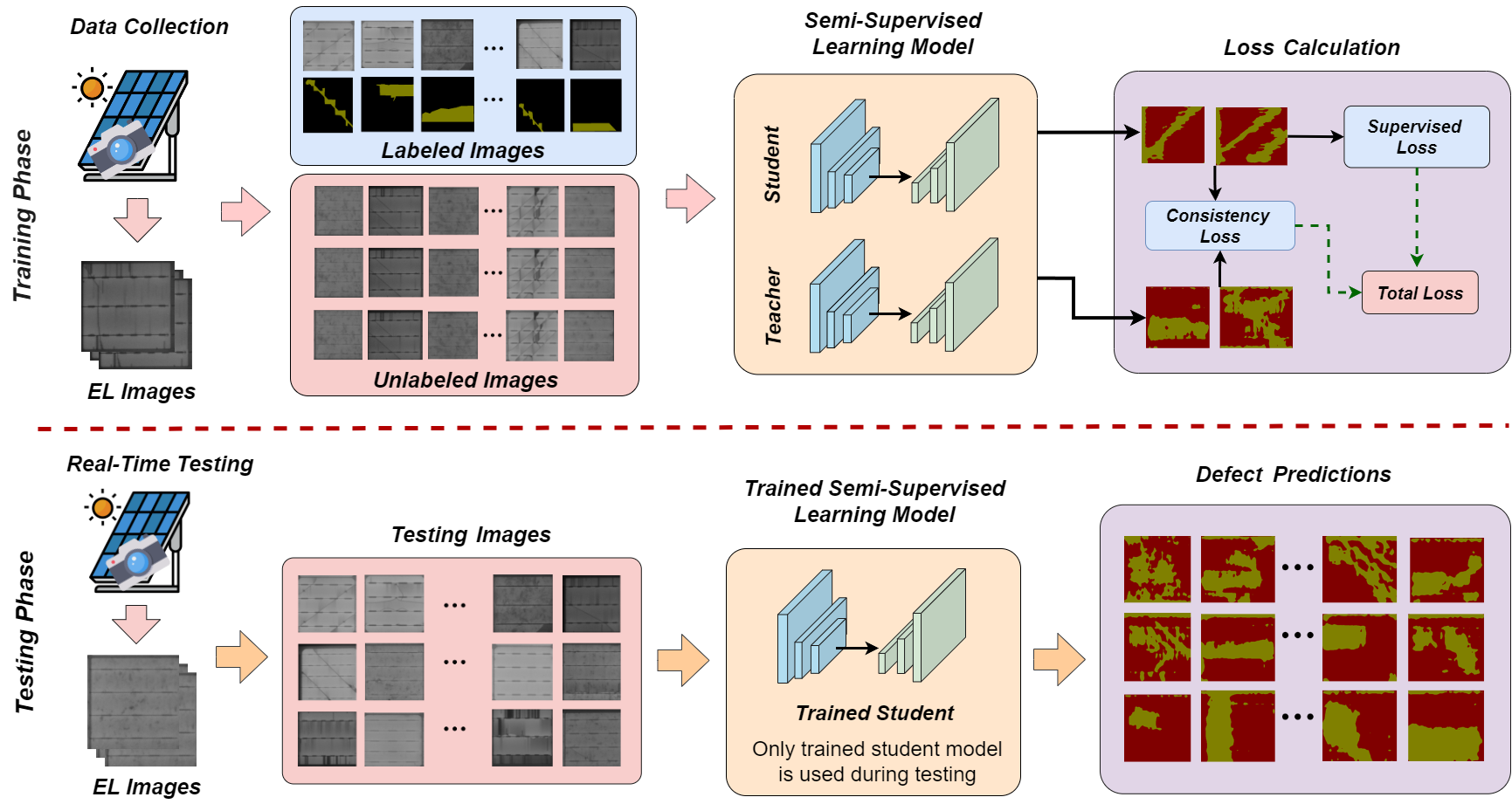
To address the challenges posed by class imbalance and the scarcity of labeled data in real-world datasets, PV-S3 employs a novel unsupervised semi-cross entropy loss function. This loss effectively leverages both labeled and unlabeled data, enhancing the model’s ability to accurately identify rare defects. Semi-cross entropy introduces stricter positive and negative thresholds, fostering stronger convergence by deferentially weighting the contributions of various classes. This mechanism ensures that the model not only learns from the limited labeled data but also extracts valuable patterns from the unlabeled data, thereby significantly improving the detection accuracy of less frequent defect types. Figure 1 represents an high-level overview of the proposed framework for defect detection in photovoltaic cells using semi-supervised segmentation.

Figure 1: An overview of the proposed semi-supervised approach for PV defect detection: It utilizes both labeled and unlabelled images in a semi-supervised framework (SSL) using supervised and unsupervised consistency losses to train the defect detection model (top row) and during testing the trained model predicts the defect class for each pixel in EL images (bottom row).

The major contributions of our research are as follows:

• We study automatic defect detection in photovoltaic cells using a novel approach where we perform semantic segmentation of PV cell defects with limited annotations. This reduces the dependency on a large amount of labeled data alleviating the need for extensive manual annotation.

• We propose PV-S3, a novel framework to solve this problem which can utilize both labeled and unlabeled samples to perform semantic segmentation for PV defect detection.

• We develop Semi-Cross-Entropy loss, a learning objective which helps PV-S3 to detect rare defects present in limited and an imbalanced training data.

• We perform extensive evaluation of our approach on several real-world PV datasets, demonstrating its effectiveness and efficiency in detecting various types of defects. The proposed approach outperforms existing state-of-the-art fully supervised methods with merely 20% annotations.

In this study, we address the challenge of employing semi-supervised learning (SSL) for automatic detection of defects in PV modules to reduce the need for extensive annotation. Our proposed method will advance the field of PV maintenance by providing an efficient, and cost-effective solution for defect detection.

2 Related Work

Defect detection in PV modules has witnessed a progression from manual inspection to advanced automated techniques. Traditional methods involving manual visual examination of EL images have limitations in scalability and subjectivity [21]. Adoption of machine learning techniques, particularly deep learning with Convolutional Neural Networks (CNNs), has enabled more accurate and efficient detection.

EL Imaging and PV Cells

PV modules are essential components for converting sunlight into electrical energy, comprised of interconnected photovoltaic cells that absorb sunlight to generate direct current (DC) electricity. However, defects introduced during manufacturing, handling, and installation processes can impair their performance and reliability. Common issues include cracks, fractures, soldering problems, corrosion, and electrical contact issues [41, 45]. These defects can lead to decreased power output, hotspots, accelerated degradation, and safety risks. Timely detection and identification of these issues are crucial for ensuring optimal PV system operation and longevity. Two primary techniques used for assessing PV module performance are current-voltage (I-V) measurements and electroluminescence (EL) imaging. EL imaging is particularly valuable for maintenance evaluations and defect detection. Given the large scale of PV plants, there is a growing focus on automating defect detection and classification in EL images [49, 36, 45].

Classification

Defect classification in PV modules is crucial for panel efficiency and longevity. Traditional machine learning methods like Support Vector Machines (SVMs) [42, 13], Random Forests [42, 9], and k-Nearest Neighbors (k-NN) [42, 35] have been widely applied, particularly effective for simpler defect types. However, the diverse and complex nature of PV defects demands more advanced techniques. Deep learning, especially Convolutional Neural Networks (CNNs), has gained prominence for its ability to learn from large datasets, capturing subtle defect variations [4, 13]. Modified CNN variants like multi-channel CNNs [54] and HRNet [55] have shown effectiveness in defect detection. Various CNN architectures, including VGG16 [46], ResNet50 [46], and InceptionV3 [46], have been explored for defect classification, leveraging multiple convolutional layers and transfer learning with pre-trained models for fine-tuning.

Segmentation

Defect detection, unlike classification, demands defect localization in images, employing segmentation techniques for precise delineation. This task is vital for understanding defect characteristics and their spatial distribution in detail. Numerous models and methodologies aim for accurate segmentation of PV cell defects [20, 40, 55]. Semantic segmentation, a robust computer vision technique, has recently gained traction for this purpose, leveraging powerful pre-trained models [20, 40]. However, training segmentation models, especially for specialized domains like PV module defect detection, poses unique challenges, primarily due to extensive data annotation requirements [37]. The effectiveness of segmentation models hinges on ample labeled data availability for training, underscoring the necessity for efficient annotation strategies.

Our research introduces a novel approach to PV module defect detection, leveraging semantic segmentation and a semi-supervised learning framework. Unlike prior works, our method efficiently incorporates both labeled and unlabeled data, enhancing model performance without heavy reliance on extensive labeled datasets.

3 Proposed Methodology

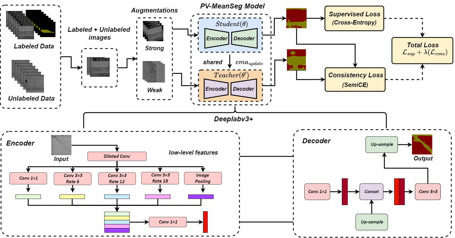
The proposed method addresses the challenge of limited labeled data in PV defect detection through semi-supervised learning. We utilize the mean-teacher approach [47], aiming to enhance defect detection accuracy and efficiency while reducing the need for extensive expert annotation. An overview of the proposed approach is shown in Figure  2 displaying the process of PV-S3 for defect detection in photovoltaic cells.

Figure 2: Overview of PV-S3 for Semantic Segmentation of PV Defects: The framework takes labeled and unlabeled images as input and both labeled and unlabeled images are given as input to both student and teacher models. The images are augmented before passing to both models where strong augmented images are given to the student network and weak augmented images to the teacher network. Deeplabv3+ is used as segmentation model for both student and teacher networks.

Given a dataset $D$ comprising labeled images $X_{L}$ with corresponding ground truth segmentation masks $Y_{L}$, and unlabeled images $X_{U}$ without associated labels, our objective is to train a model $M$ capable of accurately generating segmentation masks for new, unseen input images. $X_{L}=\{X_{L}^{1},X_{L}^{2},...,X_{L}^{N}\}$ represents the set of $N$ labeled images, with $Y_{L}=\{Y_{L}^{1},Y_{L}^{2},...,Y_{L}^{N}\}$ denoting the corresponding segmentation masks indicating defect present and type. $X_{U}=\{X_{U}^{1},X_{U}^{2},...,X_{U}^{K}\}$ denotes unlabeled images, where $K$ is their count. These images lack ground truth masks but are utilized by the model to learn from unlabeled data through semi-supervised techniques. The primary output comprises predicted segmentation masks $\hat{Y}$ for input images $X$, with each mask $\hat{Y}^{i}$ corresponding to the model’s prediction for $X^{i}$. Model $M$ aims to output pixel-wise classifications indicating the likelihood of each pixel belonging to various defect types.

3.1 Background

Semi-supervised learning utilizes both labeled and unlabeled data thus filling gaps in conventional supervised learning. It leverages abundant unlabeled data to enhance model’s performance. The Mean Teacher framework [47] is the key here, employing a student network $S(\theta)$ and a teacher network $T(\theta^{\prime})$. The teacher network’s weights are updated based on the student network through exponential moving average, facilitating pseudo-labeling for unlabeled data. This integration improves learning outcomes by guiding the student to match teacher predictions on labeled data and learn from them on unlabeled data, enhancing model generalization. This approach is especially valuable with limited labeled data, allowing learning from both labeled samples and larger unlabeled datasets. For segmentation tasks, the Mean Teacher framework extends to pixel-wise labeling [34], with the teacher’s pixel-wise predictions serving as soft labels for unlabeled images. This guidance aids the student in learning the spatial layout of classes, improving segmentation accuracy.

3.2 Proposed Approach

PV-S3 is a semi-supervised learning framework leveraging both labeled and unlabeled data to enhance defect detection. It employs a dual-network system: a student network $S(\theta)$ and a teacher network $T(\theta^{\prime})$. The teacher network guides the student using pseudo-labels generated from its predictions on unlabeled data $X_{U}$, enabling the student network to learn complex defect patterns without explicit annotations. PV-S3 utilizes two loss functions: cross-entropy for labeled data and Semi Cross-Entropy (SemiCE) loss for unlabeled data, enhancing predictive consistency. PV-S3 adopts the DeepLabv3+ architecture with pre-trained ResNet50 weights, featuring an encoder-decoder architecture with atrous convolutions for multi-scale contextual information extraction. The model is trained with the mean teacher approach, updating student parameters via gradient descent and refining teacher parameters with Exponential Moving Average (EMA). This ensures stable guidance and improved generalization.

The algorithm  1 outlines PV-S3’s semi-supervised defect detection in solar PV modules. It begins with labeled data $(X_{L},Y_{L})$, unlabeled data $X_{U}$, and hyperparameters such as $\lambda$, $\alpha$, and epochs, producing the trained student model $S(\theta^{\prime})$. Student and teacher networks $S(\theta)$ and $T(\theta^{\prime})$ are initialized with same pretrained weights. For each epoch, mini-batches $M_{L}$ and $M_{U}$ are sampled from labeled and unlabeled datasets to get training samples ($M_{L}$, $M_{U}$). Strong and weak augmentations are applied to these training samples to get ($M_{L}^{\prime\prime}$, $M_{U}^{\prime\prime}$) and ($M_{L}^{\prime}$, $M_{U}^{\prime}$). ($M_{L}^{\prime\prime}$, $M_{U}^{\prime\prime}$) is passed to the Student network and ($M_{L}^{\prime}$, $M_{U}^{\prime}$) is passed to the Teacher network. Losses $\mathcal{L}_{S}$ and $\mathcal{L}_{U}$ for labeled and unlabeled data are computed using Cross-Entropy and SemiCE functions. Total loss $\mathcal{L}_{total}$, a weighted sum, balances both losses with $\lambda$. Student parameters update via backpropagation based on total loss, while teacher parameters refine using EMA with decay rate $\alpha$.

Algorithm 1 PV-S3: Semi-Supervised Learning for PV Module Defect Detection

1:  $Input:(X_{L},Y_{L}),X_{U}$ {Labeled and unlabeled images}

2:  $Hyperparameters:\lambda,\alpha,\text{epochs}$ {Hyperparameters for training}

3:  $Output:$ $S(\theta^{\prime})$ {Trained Student network}

4:  Initialize $S(\theta),T(\theta^{\prime})$ {Initialize networks}

5:  for $epoch=1$ to epochs do

6:     for each $batch$ in training batches do

7:        $M_{L}\leftarrow$ sample from $(X_{L},Y_{L})$ {Sample labeled mini-batch}

8:        $M_{U}\leftarrow$ sample from $X_{U}$ {Sample unlabeled mini-batch}

9:        $(M_{L}^{\prime},M_{U}^{\prime})\leftarrow$ apply weak augmentation to $(M_{L},M_{U})$ {Augment mini-batch}

10:        $(M_{L}^{\prime\prime},M_{U}^{\prime\prime})\leftarrow$ apply strong augmentation to $(M_{L},M_{U})$ {Augment mini-batch}

11:        $(P_{S}L,P_{S}U)\leftarrow S(M_{L}^{\prime\prime},M_{U}^{\prime\prime})$ {Compute student predictions on $(M_{L}^{\prime\prime},M_{U}^{\prime\prime})$}

12:        $(P_{T}L,P_{T}U)\leftarrow T(M_{L}^{\prime},M_{U}^{\prime})$ {Compute teacher predictions on $(M_{L}^{\prime},M_{U}^{\prime})$}

13:        $\mathcal{L}_{S}\leftarrow\text{CrossEntropy}((P_{S}L,Y_{L})$ {Supervised loss for labeled data}

14:        $\mathcal{L}_{U}\leftarrow\text{SemiCrossEntropy}(<P_{S}U,P_{S}L>,<P_{T}U,P_{T}U>)$ {Unsupervised loss}

15:        $\mathcal{L}\leftarrow\mathcal{L}_{S}+\lambda\mathcal{L}_{U}$ {Total loss}

16:        Update $S$ using $\nabla L$ {Update student network}

17:        $\theta^{\prime}\leftarrow\alpha\theta^{\prime}+(1-\alpha)\theta$ {Update teacher with EMA}

18:     end for

19:  end for

3.2.1 Supervised Loss

In the context of the mean teacher network, crucial for defect detection in EL images, the optimization of the supervised loss, along with the consistency loss, is emphasized. The supervised loss is vital, aiming to reduce the difference between the student network’s pixel-wise predictions and the actual segmentation masks, which are the ground truth for the labeled dataset.

The supervised loss for this semantic segmentation task is computed using the cross-entropy loss function. which involves making predictions at the pixel level across multiple classes or defect types. The supervised loss is formulated as follows:

$$\mathcal{L}_{supervised}=-\frac{1}{N_{L}}\sum_{i=1}^{N_{L}}\sum_{c=1}^{C}\sum_{p=1}^{P}Y_{labeled}^{i,p}(c)\log(P_{student}^{i,p}(c))$$ (1)

Here, $N_{L}$ represents the total number of labeled images in the dataset, $C$ denotes the number of defect types, and $P$ is the total number of pixels in each image. The term $Y_{labeled}^{i,p}(c)$ indicates whether class $c$ is present at pixel $p$ for the $i$-th instance, and $P_{student}^{i,p}(c)$ reflects the student model’s predicted probability that pixel $p$ in instance $i$ belongs to class $c$.

3.2.2 Consistency Loss

The consistency loss ensures uniformity between student and teacher network predictions by comparing their outputs on labeled and unlabeled data. In the standard mean teacher framework, Mean Square Error (MSE) typically serves as the consistency loss, aiming to minimize prediction discrepancies across datasets. However, MSE may not adequately address the complexities of defect detection in photovoltaic cells, especially concerning class imbalance and limited labeled data. To address these challenges, we introduce the SemiCE Loss tailored for semi-supervised defect detection. SemiCE enhances learning in scenarios of data scarcity and class imbalance, focusing on differential treatment of positive and negative predictions across labeled and unlabeled data.

The SemiCE loss consists of two key components: the positive loss ($\mathcal{L}_{\text{pos}}$) and the negative loss ($\mathcal{L}_{\text{neg}}$). $\mathcal{L}_{\text{pos}}$ emphasizes improving the accuracy of positive predictions crucial for defect identification. Conversely, $\mathcal{L}_{\text{neg}}$ handles negative predictions below the confidence threshold to prevent excessive noise interference. Integrating SemiCE within the mean teacher framework enhances training stability and effectiveness. By optimizing positive and negative predictions while considering unlabeled data characteristics, SemiCE fosters accurate defect detection in solar PV modules.

The $\mathcal{L}_{\text{pos}}$ represents the loss associated with confident positive predictions. These are predictions where the model assigns a high probability to the correct class and the input’s confidence exceeds a certain threshold ($t_{\text{pos}}$). In mathematical terms it is formulated as :

$$\mathcal{L}_{\text{pos}}=-\frac{1}{N_{\text{U}}}\sum_{i=1}^{N_{\text{U}}}\sum_{j=1}^{H\times W}\begin{cases}Y_{\text{L},ij}\cdot\log\left(\frac{\exp(P_{\text{$\theta$},ij})}{\sum_{k=1}^{H\times W}\exp(P_{\text{$\theta$},ik})}\right),&\text{if }Y_{\text{L},ij}=1\text{ and }P_{\text{$\theta$},ij}\geq t_{\text{pos}}\\ 0,&\text{otherwise}\end{cases}$$ (2)

On the other hand, $\mathcal{L}_{\text{neg}}$ accounts for negative predictions below the confidence threshold. This threshold is set as $t_{\text{neg}}$ and is typically chosen to ensure that only highly confident negative predictions contribute to the loss. In mathematical terms:

$$\mathcal{L}_{\text{neg}}=-\frac{1}{N_{\text{U}}}\sum_{i=1}^{N_{\text{U}}}\sum_{j=1}^{H\times W}\begin{cases}(1-Y_{\text{L},ij})\cdot\log\left(\frac{\exp(-P_{\text{$\theta$},ij})}{\sum_{k=1}^{H\times W}\exp(-P_{\text{$\theta$},ik})}\right),&\text{if }Y_{\text{L},ij}=0\text{ and }P_{\text{$\theta$},ij}<-t_{\text{neg}}\\ 0,&\text{otherwise}\end{cases}$$ (3)

The final Semi Cross Entropy Loss $\mathcal{L}_{\text{SemiCE}}$ is the sum of $\mathcal{L}_{\text{pos}}$ and $L_{\text{neg}}$: The SemiCE loss is the same as the Consistency loss ($\mathcal{L}_{\text{cons}})$ for the student-teacher framework where this loss component tries to make the predictions of the student model consistent.

$$\mathcal{L}_{\text{cons}}=\mathcal{L}_{\text{SemiCE}}=\mathcal{L}_{\text{pos}}+\mathcal{L}_{\text{neg}}$$ (4)

In the equations, $N_{\text{U}}$ represents the total number of unlabeled images, $P_{\text{$\theta$}_{i}(j)}$ represent the logits predicted by the model, targets are the ground truth labels, $Y_{\text{L}_{i}(j)}$ is the ground truth label for the $i$-th sample and $j$-th class, and $H\times W$ represents the spatial dimensions of the image.

The overall loss function for the mean teacher network is a combination of the supervised loss and the consistency loss, weighted by respective coefficients. It can be represented in Equation 5 as:

$$\mathcal{L}_{\text{total}}=\mathcal{L}_{\text{sup}}+\lambda\mathcal{L}_{\text{cons}}$$ (5)

where $\lambda$ is the weighting coefficient that determines the importance of the consistency loss relative to the supervised loss.

3.2.3 Augmentations

Augmentations play a crucial role in enhancing the model’s ability to detect defects in solar cells by introducing controlled variations to the training data. These variations enable the model to adapt to diverse real-world scenarios, capturing the nuances of defects under different conditions, thus contributing to improved accuracy and robustness in defect detection. PV-S3 utilizes both weak and strong augmentations to enrich the diversity of training data. Weak augmentations introduce subtle variations like random rotations and flips, enhancing the model’s capability to recognize defects across various orientations and lighting conditions. Strong augmentations, on the other hand, involve significant alterations to training images, challenging the model to adapt to complex scenarios beyond typical conditions. While weak augmentations are applied to the teacher model for generating better pseudo-labels, strong augmentations are used for training the student model, exposing it to more challenging samples to enhance its ability to generalize from complex variations, thus improving overall performance and robustness.

4 Experiments and Evaluation

Datasets

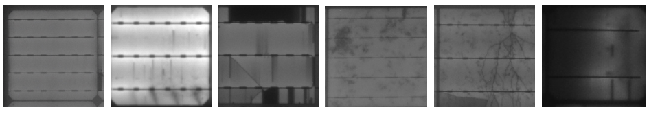
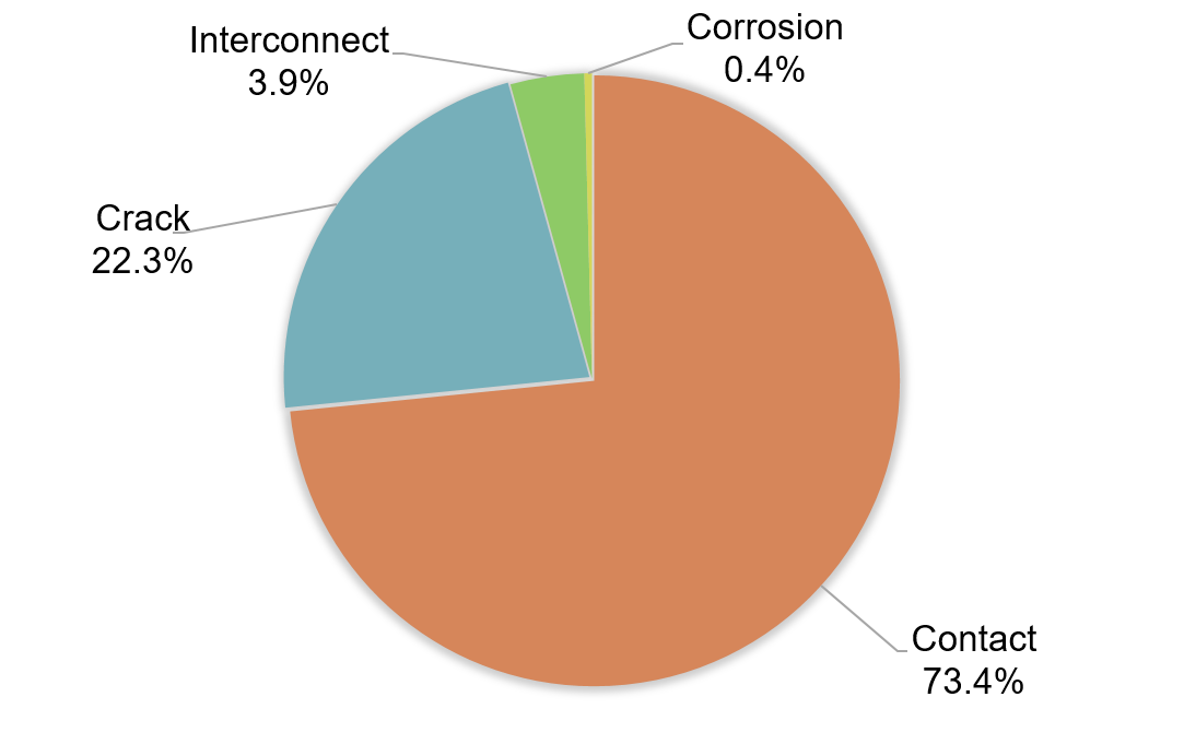
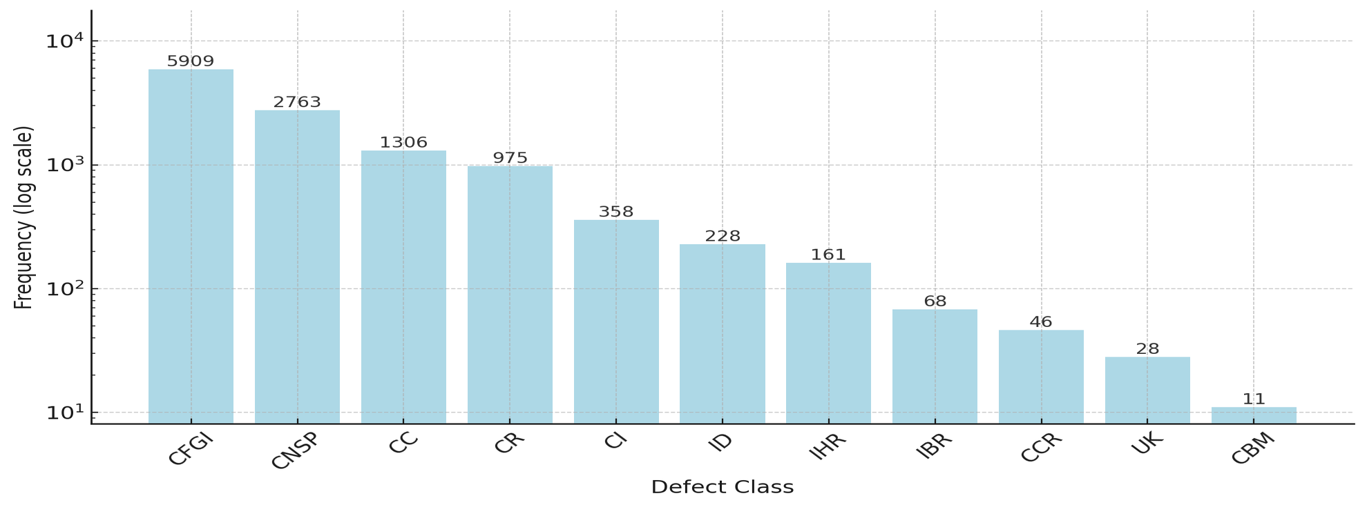
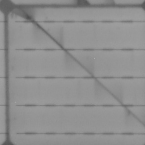
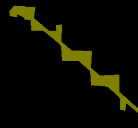
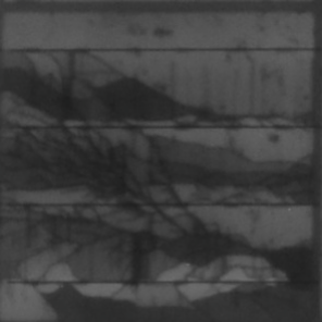
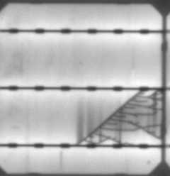
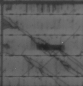
We use the UCF-EL Defect Dataset, which includes nine distinct defect types, each with specific EL patterns and locations on the cell surface, such as cracks, grid interruptions, and corrosion. In Figure  3, we present a visual representation of some of the EL images containing defects. The defect are classified into four major defect classes which are Contact, Crack, Interconnect and Corrosion. Further each of these defects have sub categories for defect. Pie charts and histogram distributions of defect classes, as shown in Figures  4 and  5, indicate Contact defects are the most prevalent, followed by Crack and Interconnect, while Corrosion defects are least common.

Figure 3: Sample defect images from UCF-EL dataset: The images from the left show defect types “Contact Near SolderPad”, “Contact Front Grid Interruption”, “Crack Isolated”, “Contact Corrosion”, “Crack Resistive” and “Interconnect Highly Resistive”.

Figure 4: Distribution of defects for UCF-EL dataset: The pie chart on the left shows the distribution of 4 defect classes in the images whereas the pixel-wise pie chart on the right further details the distribution of defects at the pixel level.

Figure 5: Distribution of fine-grained defect classes for UCF-EL dataset: Each defect is denoted by an abbreviation for clarity. “CNSP” represents Contact Near Solder Pad, “CR” stands for Crack Resistive, “CFGI” is Contact Front Grid Interruption, “CC” denotes Crack Closed, “CI” indicates Crack Isolated, “IHR” means Interconnect Highly Resistive, “IBR” stands for Interconnect Bright Spot, “CCR” is Contact Corrosion, “UK” signifies Unknown defects, “CBM”represents Contact Belt Marks, and “ID” denotes Interconnect Disconnected.

In addition to the primary UCF-EL dataset, our study uses different datasets to validate the model’s performance evaluation and its ability to generalize across various scenarios. The study performed by [40] used a combination of different datasets containing EL images from five different sources [29, 14, 12, 8]. We call this combined dataset as Combined Solar Benchmark dataset (CSB-Dataset). This dataset is further divided into three subsets, Subset 1 (CSB-Dataset-S1) contains 593 images with 12 defect classes, Subset 2 (CSB-Dataset-S2) contains 2109 images with 15 defect classes and Subset 3 (CSB-Dataset-S3) contains 2282 images with 16 defect classes. Out of all these defect classes, the major defect classes are Crack, Gridline, and Inactive, and we focus on these three defect types in our experiments which also enables a fair comparison with [40].

Training Details

During the training phase, the model is trained with 20% of the labeled data and 80% of the unlabeled data from the training set. The training process involves an iterative optimization approach, where the model is trained using both labeled and unlabeled data in a semi supervised manner. The labeled data is used to compute the standard supervised loss, while the unlabeled data is employed to calculate a consistency loss, ensuring that the model produces consistent predictions for similar inputs. The training process is carried out for 30 epochs with batch size 16, Stochastic Gradient Descent (SGD) optimizer with learning rate 0.001, weight decay 0.0001 and momentum 0.9 on a 32GB GPU. Further consistency weight is taken as 1.5 and base size of image is $299\times 299$ and crop size of $224\times 224$.

Evaluation Metric

We evaluate the proposed method using Mean Intersection over Union (IoU), precision, recall, and F1 score. Mean IoU measures the overlap between the predicted segmentation masks and the ground truth annotations, providing an overall assessment of the segmentation accuracy. Precision represents the ratio of correctly predicted defect pixels to all predicted defect pixels, while recall measures the proportion of correctly predicted defect pixels out of all ground truth defect pixels. F1 score combines precision and recall, providing a balanced measure of the model’s overall performance.

4.1 Quantitative Evaluation

Our quantitative analysis focused on the performance of PV-S3 with 20% labeled data in defect detection. By comparing the model’s predictions with fully-supervised learning and the baseline model for supervised learning with 20% labeled data along with semi-supervised learning with 100% labeled data, we assess the model’s performance in identifying and segmenting defects corresponding ground truths.

Comparison under limited labels

Regarding the performance on UCF-EL dataset with the semi-supervised learning scenario with 20% labeled data, we record average values for metrics as IoU of 67%, precision of 88.90%, recall of 72.50%, and F1-score of 78.17% whereas with 20% labeled data in the supervised learning yielded mean IoU of 8.76%, precision of 26.27%, recall of 25.79% and F1-score of 14.73%. Based on the results we can observe that semi-supervised learning with PV-S3 has yielded significant improvement in results as compared to fully supervised learning with same amount of labeled dataset. The scores with the baseline model of supervised learning with 20% labeled data and semi-supervised learning with 20% labeled data has been summarized in Table  1. To further evaluate the robustness of PV-S3, we perform three experimental runs with different subsets of labeled samples which are randomly selected from the training dataset. The mean and standard deviation of performance metrics for each defect class are shown in Table  2. We observe that the proposed SSL approach significantly outperform the supervised baseline in all metrics consistently, demonstrating its robustness.

	IoU		Precision		Recall		F1-Score
Defect Class	SL (20%)	SSL (20%)	SL (20%)	SSL (20%)	SL (20%)	SSL (20%)	SL (20%)	SSL (20%)
Crack	25.29	89.00	26.66	89.75	83.13	98.00	40.37	93.69
Contact	6.89	49.00	10.49	79.50	16.73	57.00	12.89	66.39
Interconnect	0.85	40.00	2.58	88.81	1.26	43.00	1.69	57.94
Corrosion	2.03	90.00	65.37	97.54	2.05	92.00	3.98	94.68
Average	8.76	67.00	26.27	88.90	25.79	72.50	14.73	78.17

Table 1: Comparison of PV-S3 under limited labels with our supervised method on UCF-EL dataset: The table shows the performance of different defect classes under Supervised Learning (SL) with 20% labeled images and Semi-Supervised Learning (SSL) with 20% labeled images. The metrics evaluated include IoU, Precision, Recall, and F1-Score, facilitating a direct comparison of the impact of labeling extent on model performance.

	IoU		Precision		Recall		F1-Score
Defect Class	SL (20%)	SSL (20%)	SL (20%)	SSL (20%)	SL (20%)	SSL (20%)	SL (20%)	SSL (20%)
Crack	$26.20\pm 0.66$	$89.05\pm 0.38$	$26.66\pm 0.63$	$90.43\pm 0.78$	$83.50\pm 1.01$	$97.97\pm 0.24$	$41.41\pm 0.73$	$94.05\pm 0.33$
Contact	$6.95\pm 0.06$	$49.95\pm 1.02$	$11.06\pm 1.55$	$77.16\pm 1.17$	$16.92\pm 0.78$	$58.52\pm 1.71$	$12.67\pm 0.89$	$66.95\pm 0.92$
Interconnect	$0.7\pm 0.26$	$41.05\pm 0.85$	$2.13\pm 0.78$	$92.07\pm 2.90$	$1.03\pm 0.38$	$42.86\pm 0.81$	$1.39\pm 0.51$	$58.46\pm 0.55$
Corrosion	$2.48\pm 0.61$	$86.09\pm 7.37$	$62.40\pm 4.86$	$92.24\pm 6.99$	$2.02\pm 0.06$	$92.62\pm 2.02$	$3.92\pm 0.13$	$92.33\pm 4.36$
Average	$9.06\pm 0.09$	$66.53\pm 1.35$	$26.53\pm 1.43$	$88.17\pm 1.94$	$25.86\pm 0.05$	$72.99\pm 0.35$	$14.85\pm 0.05$	$78.00\pm 0.78$

Table 2: Robustness of PV-S3 with variation on data sampling: Three runs are conducted for supervised learning with 20% labeled images and semi-supervised learning with 20% labeled images, and mean and standard deviation are recorded for performance metrics for each defect class along with their average values. This assessment allows for direct comparison between SL and SSL approaches for each metric.

Comparison with fully labeled dataset

With 100% labeled data using fully supervised learning, the Deeplabv3+ model achieves mean metrics of IoU: 70.84%, precision: 86.29%, recall: 80.12%, and F1-score: 82.03% (Table  3). Comparing these results with our 20% labeled semi-supervised learning approach, PV-S3 yields comparable results to fully supervised learning, with even higher precision. Leveraging 100% labeled data in the semi-supervised framework with PV-S3 significantly improves performance, yielding mean IoU: 74.75%, precision: 91.30%, recall: 79.96%, and F1-score: 84.24%. This improvement underscores the benefits of a larger dataset in better understanding and segmenting defects in PV module EL images.

	IoU		Precision		Recall		F1-Score
Defect Class	FSL (100%)	SSL (100%)	FSL (100%)	SSL (100%)	FSL (100%)	SSL (100%)	FSL (100%)	SSL (100%)
Crack	88.38	91.78	90.94	93.96	96.91	97.54	93.83	95.72
Contact	52.92	58.29	80.75	78.70	60.56	69.20	69.21	73.65
Interconnect	59.70	53.89	90.70	94.93	63.59	55.49	74.76	70.04
Corrosion	82.39	95.26	82.78	97.62	99.43	97.61	90.34	97.57
Average	70.84	74.75	86.29	91.30	80.12	79.96	82.03	84.24

Table 3: Comparison of PV-S3 with our fully supervised method on UCF-EL dataset: The table shows the performance of different defect classes under Semi Supervised Learning (SSL) with 100% labeled images, and Fully Supervised Learning (FSL) with 100% labeled images. The metrics evaluated include IoU, Precision, Recall, and F1-Score, facilitating a direct comparison of the impact of labeling extent on model performance.

Baselines	Labeled Data (%)	IoU (%)	Precision (%)	Recall (%)	F1-Score (%)
Deeplabv3 [20]	$100$	$57.30$	$59.00$	$59.75$	$57.75$
Deeplabv3+ (Ours SL)	$100$	$63.66$	$75.33$	$79.66$	$76.66$
PV-S3 (Ours-SSL (20%))	$20$	$67.00$	$88.90$	$72.50$	$78.17$
PV-S3 (Ours-SSL (100%))	$100$	$74.75$	$91.30$	$79.96$	$84.24$

Table 4: Comparison of PV-S3 with existing supervised approaches on UCF-EL dataset: Fully Supervised Learning with 100% labeled data using Deeplabv3/Deeplabv3+ and Semi-Supervised Learning using Deeplabv3+ (Ours-SSL(20%)) with 20% labeled images and Semi-Supervised Learning using Deeplabv3+ with 100% labeled data (Ours-SSL(100%)). PV-S3 performed better in terms of all four key metrics significantly reducing the annotation cost.

Comparisons with existing Fully Supervised learning on UCF-EL dataset, performed by [20], across key metrics are summarized in Table  4. We observe improved performance with merely 20% labeled samples and significant enhancement in IoU, Precision, and F1-Score using all labeled samples. Our approach, utilizing just 20% of labeled samples, yields a notable absolute enhancement, including a 9.7% increase in IoU, a 29.9% rise in Precision, a 12.75% boost in Recall, and a 20.42% improvement in F1-Score compared to the previous state-of-the-art supervised method, reducing annotation expenses by 80%.

Experiment		IoU (%)		Precision (%)		Recall (%)		F1-Score (%)
Dataset	Defect Type	SSL (20%)	FSL (100%)	SSL (20%)	FSL (100%)	SSL (20%)	FSL (100%)	SSL (20%)	FSL (100%)
CSB-Dataset-S1	Crack	$50.00$	$58.00$	$57.00$	$64.00$	$80.00$	$86.00$	$66.00$	$73.00$
	Gridline	$74.00$	$83.00$	$82.00$	$91.00$	$88.00$	$91.00$	$85.00$	$91.00$
	Inactive	$50.00$	$50.00$	$68.00$	$71.00$	$66.00$	$62.00$	$67.00$	$66.00$
	Average	$58.00$	$63.67$	$69.00$	$75.33$	$78.00$	$79.67$	$72.67$	$76.67$
CSB-Dataset-S2	Crack	$61.00$	$56.00$	$78.00$	$71.00$	$74.00$	$72.00$	$76.00$	$71.00$
	Gridline	$78.00$	$84.00$	$87.00$	$92.00$	$88.00$	$91.00$	$87.00$	$91.00$
	Inactive	$62.00$	$60.00$	$70.00$	$73.00$	$86.00$	$77.00$	$77.00$	$75.00$
	Average	$67.00$	$66.67$	$78.33$	$78.67$	$82.67$	$80.00$	$80.00$	$79.00$
CSB-Dataset-S3	Crack	$55.00$	$60.00$	$84.00$	$73.00$	$62.00$	$76.00$	$71.00$	$75.00$
	Gridline	$77.00$	$85.00$	$88.00$	$90.00$	$86.00$	$93.00$	$87.00$	$92.00$
	Inactive	$62.00$	$60.00$	$65.00$	$87.00$	$86.00$	$90.00$	$75.00$	$83.00$
	Average	$64.67$	$68.33$	$79.00$	$83.33$	$78.00$	$86.33$	$77.67$	$83.33$

Table 5: Comparison with our supervised baselines on CSB-Dataset: Here we use the PV-S3 on Combined Solar Benchmark dataset (CSB-Dataset) to compare the scores of semi-supervised learning with fully supervised learning (FSL) across four key metrics.

Comparison on Combined Solar Benchmark Dataset

On the Combined Solar Benchmark Dataset (CSB-Dataset) we evaluate PV-S3 on all three subsets with three major defect classes Crack, Gridline and Inactive. The results for four key metrics, IoU, Precision, Recall and F1-Score, are summarized in Table  5. We observe competitive performance with PV-S3 using only 20% labeled samples across all metrics when compared with fully supervised method using 100% labeled samples. We also compare the performance of PV-S3 with existing methods on these datasets. This comparison is shown in Table  6. The performance of PV-S3 is compared with various baseline models which include PSPNet, UNet-12 and UNet-25 using both 20% (Our-SSL) and 100% (Our-FSL) labels. We observe that conventional semantic segmentation models like PSPNet and UNet variants which are UNet-12 and UNet-25 performed poorly in terms of the Intersection of Union as compared to Deeplab variants. In terms of recall score, UNet-25 has yielded the highest recall score of 60.66% while PSPNet yielded the lowest score of 43.0%. We observe that PV-S3 outperforms other baseline models in terms of all metric scores. Using merely 20% of labeled images for training we observed an increase of 30% in IoU and a 3% increase in recall with a reduction in 80% annotation cost compared to the state-of-the-art model on CSB-Dataset, further using our model with 100% labeled images an increase of 35.67% in IoU and 4.67% increase in recall was observed with state-of-the-art model on CSB-Dataset.

Baseline Models	Labeled Data (%)	IoU (%)	Precision (%)	Recall (%)	F1-Score (%)
PSPNet [40]	$100$	$14.00$	-	$43.00$	-
UNet-12 [39]	$100$	$16.00$	-	$58.00$	-
UNet-25 [39]	$100$	$13.33$	-	$60.67$	-
Deeplabv3+ [40]	$100$	$28.00$	-	$75.00$	-
PV-S3 (Ours-FSL)	$100$	$63.67$	$75.33$	$79.67$	$76.67$
PV-S3 (Ours-SSL)	$20$	$58.00$	$69.00$	$78.00$	$72.67$

Table 6: Comparison with existing supervised methods on CSB-Dataset-S1: We compare the results of PV-S3 with different variations with other baselines for the CSB-Dataset-S1. Deeplabv3+ with 100% labeled data (Ours-FSL) and Deeplabv3+ (Ours-SSL) with 20% labeled images performed significantly better in terms of IoU and Recall scores.

4.2 Discussion and Analysis

We further study some key aspects such as effectiveness of Semi Cross-Entropy (SemiCE) loss in addressing class imbalance, impact of variations in the amount of labeled data on our model’s performance, and the confidence level of our model in segmenting defects.

Analysing SemiCE Loss for Class Imbalance

A significant challenge in our framework was detecting interconnect defects, which, despite their small image count proportion, constitute a notable pixel distribution percentage, emphasizing the need for precise detection. We experimented with adjusting the Semi Cross-Entropy (SemiCE) thresholds to improve the detection of interconnect defects. The adaptation of Semi Cross-Entropy (SemiCE) positive and negative thresholds is a key aspect of our method. The positive threshold, when set lower, includes predictions with lesser confidence, potentially identifying more defects but risking false positives. A higher positive threshold, on the other hand, demands greater confidence for predictions to be considered positive, thus enhancing accuracy. The negative threshold, conversely, focuses on confidently negative predictions. Setting an appropriate negative threshold ensures that only highly confident negative predictions are considered, avoiding undue focus on uncertain negatives and maintaining the robustness of the defect detection process.

Threshold	Crack				Contact				Interconnect				Corrosion
	IoU	Prec	Rec	F1	IoU	Prec	Rec	F1	IoU	Prec	Rec	F1	IoU	Prec	Rec	F1
0.0, 0.0	89	93	95	94	51	71	65	68	50	65	71	78	92	94	98	96
0.2, 0.4	89	92	96	94	53	78	63	70	64	83	74	78	81	88	91	89
0.3, 0.2	89	91	98	94	52	77	61	68	44	79	50	61	67	96	69	80
0.4, 0.2	91	93	97	95	52	73	64	68	45	81	48	62	76	98	77	86
0.5, 0.5	91	93	98	95	53	75	64	69	46	97	46	63	85	97	87	92
0.6, 0.0	89	90	98	94	49	79	57	66	40	89	43	58	90	97	92	95

Table 7: Variation of performance across different thresholds: This table shows the percentages for IoU, Precision, Recall, and F1-Score for the defect classes of Crack, Contact, Interconnect, and Corrosion across different thresholds. Best overall performance of the model is highlighted with green.

In our experiments, we varied both the SemiCE positive and negative thresholds to observe their impact on Interconnect defect class performance. Performance with different thresholds is shown in Table 7, with original results in Table  1 using initial thresholds of 0.6 (positive) and 0 (negative), chosen for their balanced nature. Through experimentation, we aimed to identify threshold values optimizing the metrics while maintaining model consistency, shedding light on the intricate relationship between prediction confidence and model performance. The best threshold values achieved were 0.2 (positive) and 0.6 (negative), yielding improved performance for the Interconnect defect class with an IoU of 64%, precision of 83%, recall of 74%, and F1-Score of 78%.

Analysing Confidence in Segmentation

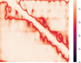
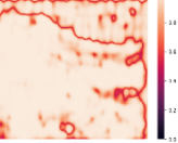
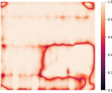
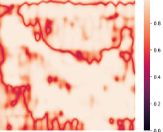
The model accurately identifies defects within regions but struggles near boundaries, as shown in Figure  6. This highlights challenges in precise boundary detection, necessitating improved boundary-aware models. While overall accuracy is good, refinement is needed for handling intricate defect details, enhancing reliability in solar PV defect detection. Our analysis of the confidence map reveals its importance in understanding prediction certainty. Overlaying it with ground truth labels and EL images enables comprehensive evaluation, pinpointing areas for improvement. Lower confidence scores around boundaries indicate detection challenges, while higher scores elsewhere demonstrate effectiveness in identifying defects. Figure  7 illustrates the confidence map’s visual representation of prediction certainty, with higher scores indicating greater confidence.

Figure 6: Visualizing semantic segmentation: Here we show visual analysis of the results obtained by PV-S3 for various defect categories. In each set of three images, the first image shows EL image, the second image is the ground-truth segmentation for corresponding defect and the third image shows the segmentation provided by PV-S3.

Figure 7: Analyzing models confidence: Here we analyse the confidence of PV-S3 for defect segmentation and observe a lower confidence in boundary regions of detected defects. In each set of three images, the first image is the EL image, the second image shows ground-truth segmentation mask, and the third image shows confidence of models prediction.

Figure 8: Performance variation with amount of labels: The plots show variation in models performance as we increase the amount of labeled samples from 5% to 20%. We observe that with merely 20% of labeled samples, the model is able to provide performance comparable to fully supervised method which use 100% labels. SSL- proposed PV-S3 approach for semi-supervised learning, SL- supervised learning with 20% labels, and FSL- fully supervised method using 100% labels.

Effect of Variation of Labeled Data in Training

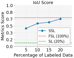
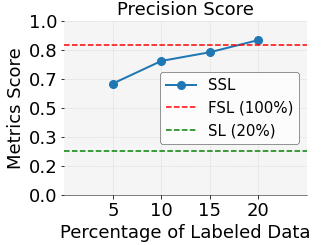
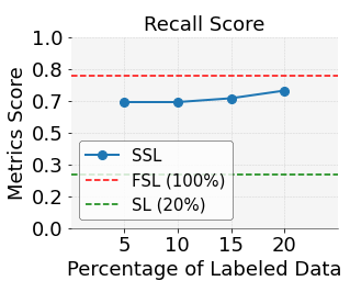
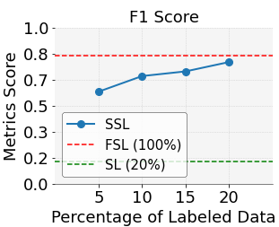
We evaluated PV-S3’s performance using different proportions of labeled data (5% to 20%) and compared it with fully supervised learning using 100% labeled data. Results in Figure  8 indicate that semi-supervised learning with 5% labeled data initially underperforms compared to fully supervised learning. However, performance notably improves at 10% labeled data and continues to increase gradually up to 20%, approaching scores achieved with 100% labeled data for IoU, Recall, and F1 score. Notably, precision scores for semi-supervised learning even exceed those of fully supervised learning.

Analysing Model Training

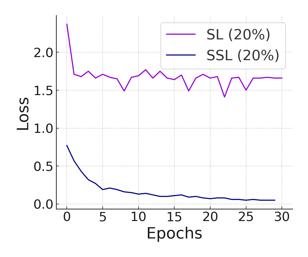
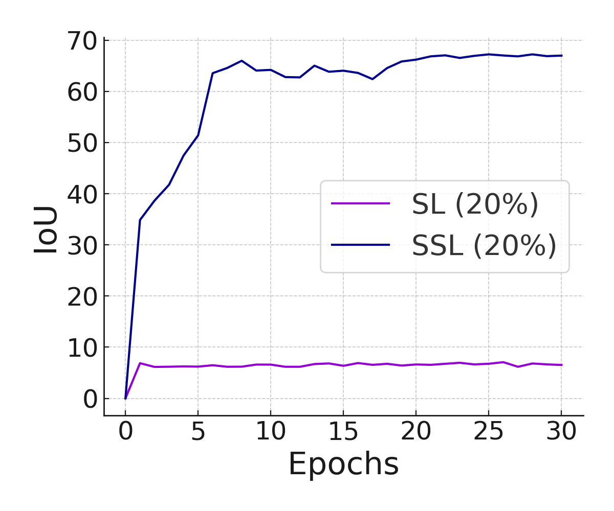
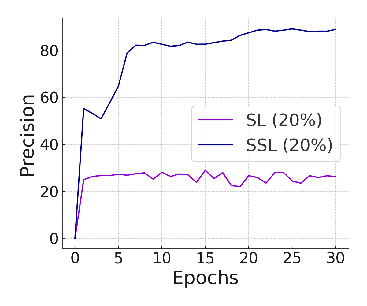
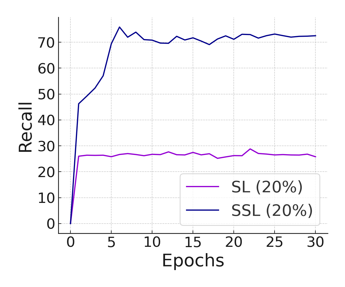
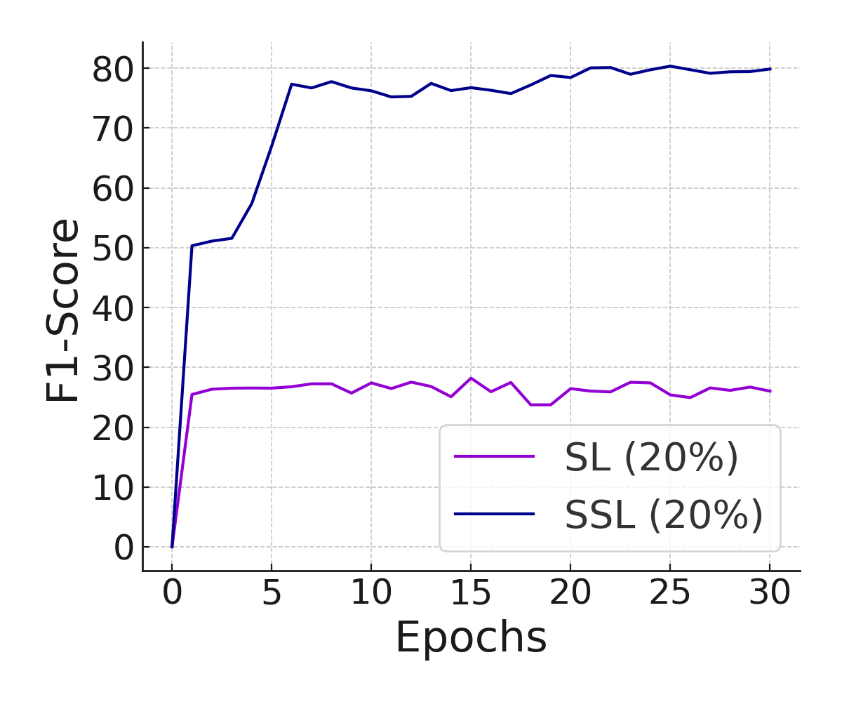
We analyze the training process of PV-S3 with epochs and compare with the supervised approach. The plots for different metrics are shown in Figure  9. Here we observe that for supervised learning with only 20% images (SL (20%)), due to less number of images and class imbalance, the model is not able to learn the features accurately and hence it has very low pixel accuracy and high loss values and have low values of precision and recall as well. For PV-S3, we observe that it reaches high values in pixel accuracy, loss, precision, and recall as training progresses.

Figure 9: Analyzing model training: The top row plots show the variation of pixel accuracy (left), loss (middle), and IoU (right) with varying training epochs, and the bottom row shows the performance metrics variation with epochs for supervised and semi-supervised learning with 20% images for precision (left), recall (middle), and F1-score (right).

Analyzing Confusion Matrix

Figure 10: Comparison of confusion matrix for supervised and semi-supervised learning: The image on the left shows the confusion matrix for supervised learning with 20% labeled images and the right image shows semi-supervised learning with 20% labeled images. The x-axis represents the true class labels and y axis represents the predicted class labels. The values are shown in the log scale for better visualization.

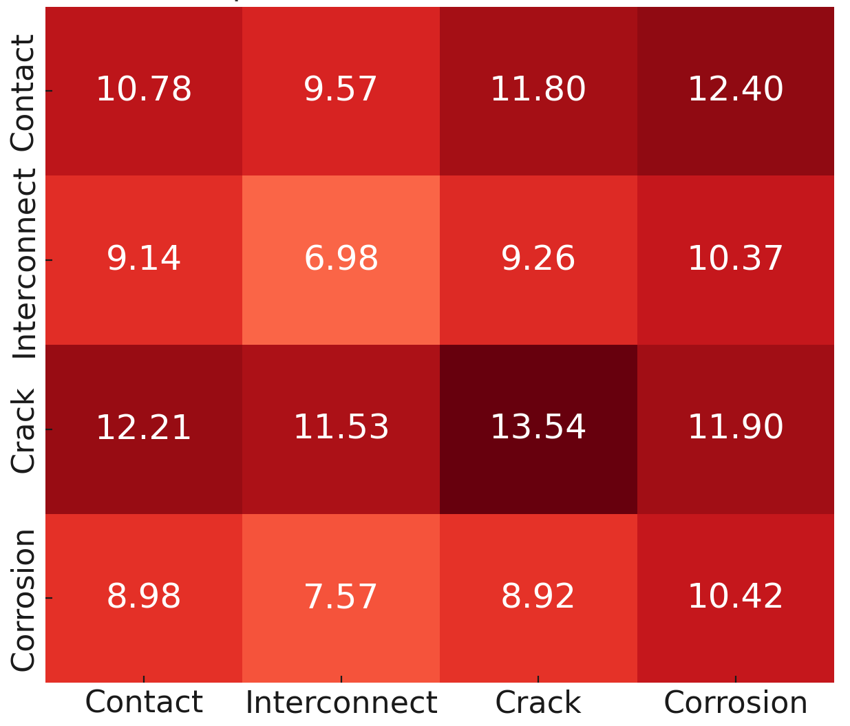
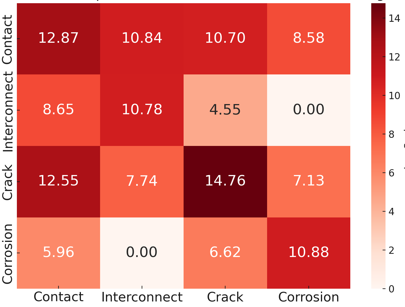
As the name suggests, using a confusion matrix we can identify the classes that are confusing for the model. We compare supervised and semi-supervised learning models’ performance using a confusion matrix (Figure 10). The supervised model misclassifies many pixels, resulting in low performance. In contrast, the semi-supervised model shows fewer misclassifications, leading to improved defect detection. The class imbalance as evident from Figure  4 introduced some bias in the predictions. Specifically, the semi-supervised model correctly classifies significantly more pixels for each defect class compared to the supervised model, indicating the effectiveness of the PV-S3 model. We observe that semi-supervised learning correctly classified 387157 (Contact), 48175 (Interconnect), 2582157 (Crack), and 53188 (Corrosion) pixels compared to the baseline (supervised) model which classified only 48050 (Contact), 1070 (Interconnect), 757701 (Crack), and 33429 (Corrosion) pixels correctly, which shows a significant improvement for PV-S3 model. However, the semi-supervised model struggles most with the contact defect class. This is due to its reliance on limited labeled data, hindering effective error propagation and feature learning. The confusion matrix in Figure 10 visually represents these findings with logarithmic values for clarity.

5 Conclusion, Limitations and Future Work

In conclusion, our research introduces PV-S3, a semi-supervised learning framework for defect detection in PV modules. PV-S3 effectively utilizes both labeled and unlabeled data, achieving accurate detection despite limited labeled samples. The proposed approach demonstrates significant potential in automating defect detection, reducing manual efforts, and enhancing the reliability of solar PV systems. The proposed approach provides mean IoU of 67%, precision of 88.75%, recall of 72.50%, and F1-score of 78.50% on one of the largest defect detection dataset with merely 20% labeled samples, significantly outperforming existing state-of-the-art method which uses 100% labeled samples.

However, our research also highlights certain limitations such as difficulty in boundary detection. While PV-S3 provides effective guidance for defect classification, accurately delineating defect boundaries can be challenging due to the defect’s complex and irregular nature.

Looking ahead, future research should focus on enhancing detection accuracy and robustness which could lead to development of tools as used for other energy tasks [51, 10]. Additionally, efforts to collect diverse unlabeled data and employ active learning strategies could enhance the model’s generalization capabilities. Furthermore, extending our approach to encompass a broader range of defect types in solar PV modules would render the system more comprehensive and adaptable to real-world scenarios. Such advancements could significantly contribute to the automation of defect detection, reducing manual labor, and ultimately enhancing the reliability of solar PV systems.

Declaration of competing interests

The authors confirm that there are no existing financial conflicts or personal connections that could potentially be perceived as influencing the outcomes or interpretations presented in this paper.

References

- [1] Ahmad Abubakar, Carlos Frederico Meschini Almeida, and Matheus Gemignani. Review of artificial intelligence-based failure detection and diagnosis methods for solar photovoltaic systems. Machines, 9(12):328, 2021.
- [2] MR Ahan, Akshay Nambi, Tanuja Ganu, Dhananjay Nahata, and Shivkumar Kalyanaraman. Ai-assisted cell-level fault detection and localization in solar pv electroluminescence images. In Proceedings of the 19th ACM Conference on Embedded Networked Sensor Systems, pages 485–491, 2021.
- [3] M Waqar Akram, Guiqiang Li, Yi Jin, and Xiao Chen. Failures of photovoltaic modules and their detection: A review. Applied Energy, 313:118822, 2022.
- [4] M Waqar Akram, Guiqiang Li, Yi Jin, Xiao Chen, Changan Zhu, Xudong Zhao, Abdul Khaliq, M Faheem, and Ashfaq Ahmad. Cnn based automatic detection of photovoltaic cell defects in electroluminescence images. Energy, 189:116319, 2019.
- [5] Jan Bauer, Otwin Breitenstein, and Jan-Martin Wagner. Lock-in thermography: a versatile tool for failure analysis of solar cells. Electronic Device Failure Analysis, 11(3):6–12, 2009.
- [6] Karl G Bedrich. Quantitative electroluminescence measurements of PV devices. PhD thesis, Loughborough University, 2017.
- [7] Martin Bliss, Xiaofeng Wu, Karl Georg Bedrich, Jake William Bowers, Thomas Richard Betts, and Ralph Gottschalg. Spatially and spectrally resolved electroluminescence measurement system for photovoltaic characterisation. IET Renewable Power Generation, 9(5):446–452, 2015.
- [8] Claudia Buerhop-Lutz, Sergiu Deitsch, Andreas Maier, Florian Gallwitz, Stephan Berger, Bernd Doll, Jens Hauch, Christian Camus, and Christoph J. Brabec. A benchmark for visual identification of defective solar cells in electroluminescence imagery. In European PV Solar Energy Conference and Exhibition (EU PVSEC), 2018.
- [9] Zhicong Chen, Fuchang Han, Lijun Wu, Jinling Yu, Shuying Cheng, Peijie Lin, and Huihuang Chen. Random forest based intelligent fault diagnosis for pv arrays using array voltage and string currents. Energy conversion and management, 178:250–264, 2018.
- [10] David Connolly, Henrik Lund, Brian Vad Mathiesen, and Martin Leahy. A review of computer tools for analysing the integration of renewable energy into various energy systems. Applied energy, 87(4):1059–1082, 2010.
- [11] Kristopher O Davis, Greg S Horner, Joshua B Gallon, Leonid A Vasilyev, Kyle B Lu, Antonius B Dirriwachter, Terry B Rigdon, Eric J Schneller, Kortan Öğütman, and Richard K Ahrenkiel. Electroluminescence excitation spectroscopy: A novel approach to non-contact quantum efficiency measurements. In 2017 IEEE 44th Photovoltaic Specialist Conference (PVSC), pages 3448–3451. IEEE, 2017.
- [12] Sergiu Deitsch, Claudia Buerhop-Lutz, Evgenii Sovetkin, Ansgar Steland, Andreas Maier, Florian Gallwitz, and Christian Riess. Segmentation of photovoltaic module cells in uncalibrated electroluminescence images. Machine Vision and Applications, 32(4), 2021.
- [13] Sergiu Deitsch, Vincent Christlein, Stephan Berger, Claudia Buerhop-Lutz, Andreas Maier, Florian Gallwitz, and Christian Riess. Automatic classification of defective photovoltaic module cells in electroluminescence images. Solar Energy, 185:455–468, 2019.
- [14] Sergiu Deitsch, Vincent Christlein, Stephan Berger, Claudia Buerhop-Lutz, Andreas Maier, Florian Gallwitz, and Christian Riess. Automatic classification of defective photovoltaic module cells in electroluminescence images. Solar Energy, 185:455–468, June 2019.
- [15] Mahmoud Dhimish. Micro cracks distribution and power degradation of polycrystalline solar cells wafer: Observations constructed from the analysis of 4000 samples. Renewable Energy, 145:466–477, 2020.
- [16] Mahmoud Dhimish and Violeta Holmes. Solar cells micro crack detection technique using state-of-the-art electroluminescence imaging. Journal of Science: Advanced Materials and Devices, 4(4):499–508, 2019.
- [17] Mahmoud Dhimish, Violeta Holmes, Bruce Mehrdadi, and Mark Dales. The impact of cracks on photovoltaic power performance. Journal of Science: Advanced Materials and Devices, 2(2):199–209, 2017.
- [18] Mahmoud Dhimish, Violeta Holmes, Bruce Mehrdadi, Mark Dales, and Peter Mather. Pv output power enhancement using two mitigation techniques for hot spots and partially shaded solar cells. Electric Power Systems Research, 158:15–25, 2018.
- [19] Jing Fan, Daliang Ju, Xiaoqin Yao, Zhen Pan, Mason Terry, William Gambogi, Katherine Stika, Junhui Liu, Wusong Tao, Zengsheng Liu, et al. Study on snail trail formation in pv module through modeling and accelerated aging tests. Solar Energy Materials and Solar Cells, 164:80–86, 2017.
- [20] Joseph Fioresi, Dylan J Colvin, Rafaela Frota, Rohit Gupta, Mengjie Li, Hubert P Seigneur, Shruti Vyas, Sofia Oliveira, Mubarak Shah, and Kristopher O Davis. Automated defect detection and localization in photovoltaic cells using semantic segmentation of electroluminescence images. IEEE Journal of Photovoltaics, 12(1):53–61, 2021.
- [21] Sara Gallardo-Saavedra, Luis Hernández-Callejo, María del Carmen Alonso-García, José Domingo Santos, José Ignacio Morales-Aragonés, Víctor Alonso-Gómez, Ángel Moretón-Fernández, Miguel Ángel González-Rebollo, and Oscar Martínez-Sacristán. Nondestructive characterization of solar pv cells defects by means of electroluminescence, infrared thermography, i–v curves and visual tests: Experimental study and comparison. Energy, 205:117930, 2020.
- [22] Francesco Grimaccia, Sonia Leva, and Alessandro Niccolai. Pv plant digital mapping for modules’ defects detection by unmanned aerial vehicles. IET Renewable Power Generation, 11(10):1221–1228, 2017.
- [23] Fiseha Mekonnen Guangul and Girma T. Chala. Solar energy as renewable energy source: Swot analysis. In 2019 4th MEC International Conference on Big Data and Smart City (ICBDSC), pages 1–5, 2019.
- [24] Sharmarke Hassan and Mahmoud Dhimish. Enhancing solar photovoltaic modules quality assurance through convolutional neural network-aided automated defect detection. Renewable Energy, 219:119389, 2023.
- [25] Humble Po-Ching Hwang, Cooper Cheng-Yuan Ku, and Mason Chao-Yang Huang. Intelligent cleanup scheme for soiled photovoltaic modules. Energy, 265:126293, 2023.
- [26] Steve Johnston. Contactless electroluminescence imaging for cell and module characterization. In 2015 IEEE 42nd Photovoltaic Specialist Conference (PVSC), pages 1–6. IEEE, 2015.
- [27] S Kajari-Schršder, Iris Kunze, and M Kšntges. Criticality of cracks in pv modules. Energy Procedia, 27:658–663, 2012.
- [28] Nadarajah Kannan and Divagar Vakeesan. Solar energy for future world:-a review. Renewable and sustainable energy reviews, 62:1092–1105, 2016.
- [29] Ahmad Maroof Karimi, Justin S Fada, Mohammad Akram Hossain, Shuying Yang, Timothy J Peshek, Jennifer L Braid, and Roger H French. Automated pipeline for photovoltaic module electroluminescence image processing and degradation feature classification. IEEE Journal of Photovoltaics, 9(5):1324–1335, 2019.
- [30] N Kellil, A Aissat, and A Mellit. Fault diagnosis of photovoltaic modules using deep neural networks and infrared images under algerian climatic conditions. Energy, 263:125902, 2023.
- [31] Thomas Kirchartz, Anke Helbig, Wilfried Reetz, Michael Reuter, Jürgen H Werner, and Uwe Rau. Reciprocity between electroluminescence and quantum efficiency used for the characterization of silicon solar cells. Progress in Photovoltaics: Research and Applications, 17(6):394–402, 2009.
- [32] Michael Koehl, Markus Heck, and Stefan Wiesmeier. Modelling of conditions for accelerated lifetime testing of humidity impact on pv-modules based on monitoring of climatic data. Solar Energy Materials and Solar Cells, 99:282–291, 2012.
- [33] Baojie Li, Claude Delpha, Demba Diallo, and A Migan-Dubois. Application of artificial neural networks to photovoltaic fault detection and diagnosis: A review. Renewable and Sustainable Energy Reviews, 138:110512, 2021.
- [34] Yuyuan Liu, Yu Tian, Yuanhong Chen, Fengbei Liu, Vasileios Belagiannis, and Gustavo Carneiro. Perturbed and strict mean teachers for semi-supervised semantic segmentation. In Proceedings of the IEEE/CVF Conference on Computer Vision and Pattern Recognition, pages 4258–4267, 2022.
- [35] Siva Ramakrishna Madeti and SN Singh. Modeling of pv system based on experimental data for fault detection using knn method. Solar Energy, 173:139–151, 2018.
- [36] Ziyao Meng, Shengzhi Xu, Lichao Wang, Youkang Gong, Xiaodan Zhang, and Ying Zhao. Defect object detection algorithm for electroluminescence image defects of photovoltaic modules based on deep learning. Energy Science & Engineering, 10(3):800–813, 2022.
- [37] Yassine Ouali, Céline Hudelot, and Myriam Tami. An overview of deep semi-supervised learning. arXiv preprint arXiv:2006.05278, 2020.
- [38] Yue Pan, Xiangdong Kong, Yuebo Yuan, Yukun Sun, Xuebing Han, Hongxin Yang, Jianbiao Zhang, Xiaoan Liu, Panlong Gao, Yihui Li, et al. Detecting the foreign matter defect in lithium-ion batteries based on battery pilot manufacturing line data analyses. Energy, 262:125502, 2023.
- [39] Lawrence Pratt, Devashen Govender, and Richard Klein. Defect detection and quantification in electroluminescence images of solar pv modules using u-net semantic segmentation. Renewable Energy, 178:1211–1222, 2021.
- [40] Lawrence Pratt, Jana Mattheus, and Richard Klein. A benchmark dataset for defect detection and classification in electroluminescence images of pv modules using semantic segmentation. Systems and Soft Computing, page 200048, 2023.
- [41] Amit Singh Rajput, Jian Wei Ho, Yin Zhang, Srinath Nalluri, and Armin G Aberle. Quantitative estimation of electrical performance parameters of individual solar cells in silicon photovoltaic modules using electroluminescence imaging. Solar Energy, 173:201–208, 2018.
- [42] Ronnie O. Serfa Juan and Jeha Kim. Photovoltaic cell defect detection model based-on extracted electroluminescence images using svm classifier. In 2020 International Conference on Artificial Intelligence in Information and Communication (ICAIIC), pages 578–582, 2020.
- [43] Amir Shahsavari and Morteza Akbari. Potential of solar energy in developing countries for reducing energy-related emissions. Renewable and Sustainable Energy Reviews, 90:275–291, 2018.
- [44] K Mohana Sundaram, Azham Hussain, P Sanjeevikumar, Jens Bo Holm-Nielsen, Vishnu Kumar Kaliappan, and B Kavya Santhoshi. Deep learning for fault diagnostics in bearings, insulators, pv panels, power lines, and electric vehicle applications—the state-of-the-art approaches. IEEE Access, 9:41246–41260, 2021.
- [45] Wuqin Tang, Qiang Yang, Zhou Dai, and Wenjun Yan. Module defect detection and diagnosis for intelligent maintenance of solar photovoltaic plants: Techniques, systems and perspectives. Energy, page 131222, 2024.
- [46] Wuqin Tang, Qiang Yang, Kuixiang Xiong, and Wenjun Yan. Deep learning based automatic defect identification of photovoltaic module using electroluminescence images. Solar Energy, 201:453–460, 2020.
- [47] Antti Tarvainen and Harri Valpola. Mean teachers are better role models: Weight-averaged consistency targets improve semi-supervised deep learning results. Advances in neural information processing systems, 30, 2017.
- [48] T Trupke, B Mitchell, JW Weber, W McMillan, RA Bardos, and R Kroeze. Photoluminescence imaging for photovoltaic applications. Energy Procedia, 15:135–146, 2012.
- [49] Du-Ming Tsai, Shih-Chieh Wu, and Wei-Chen Li. Defect detection of solar cells in electroluminescence images using fourier image reconstruction. Solar Energy Materials and Solar Cells, 99:250–262, 2012.
- [50] FJ Vorster and EE Van Dyk. High saturation solar light beam induced current scanning of solar cells. Review of scientific instruments, 78(1), 2007.
- [51] Cyril Voyant and Gilles Notton. Solar irradiation nowcasting by stochastic persistence: A new parsimonious, simple and efficient forecasting tool. Renewable and Sustainable Energy Reviews, 92:343–352, 2018.
- [52] Tzu-Kuei Wen and Ching-Chung Yin. Crack detection in photovoltaic cells by interferometric analysis of electronic speckle patterns. Solar energy materials and solar cells, 98:216–223, 2012.
- [53] Carolina M Whitaker, Benjamin G Pierce, Ahmad Maroof Karimi, Roger H French, and Jennifer L Braid. Pv cell cracks and impacts on electrical performance. In 2020 47th IEEE Photovoltaic Specialists Conference (PVSC), pages 1417–1422. IEEE, 2020.
- [54] Xiong Zhang, Yawen Hao, Hong Shangguan, Pengcheng Zhang, and Anhong Wang. Detection of surface defects on solar cells by fusing multi-channel convolution neural networks. Infrared Physics & Technology, 108:103334, 2020.
- [55] Xiaolong Zhao, Chonghui Song, Haifeng Zhang, Xianrui Sun, and Jing Zhao. Hrnet-based automatic identification of photovoltaic module defects using electroluminescence images. Energy, 267:126605, 2023.