Stability of the Abstract Thermoelastic System with Singularity

Abstract

In this paper, we analyze an abstract thermoelastic system, where the heat conduction follows the Cattaneo law. Zero becomes a spectrum point of the system operator when the coupling and thermal damping parameters of system satisfy specific conditions. We obtain the decay rates of solutions to the system with or without the inertial term. Furthermore, the decay rate of the system without inertial terms is shown to be optimal.

Key words:  thermoelastic system, stability, inertial term, singularity.

AMS subject classifications:   35Q74, 74F05.

1 Introduction

In this paper, we study an abstract thermoelastic system in which the heat conduction follows the Cattaneo law. The Cattaneo law ([4, 17]) describes finite heat propagation speed in a medium, which resolves the paradox of infinite speed of heat transfer in Fourier law and characterizes the wave-like motion of heat, known as the second sound in physics. The abstract thermoelastic system reads as follows:

$$\left\{\begin{array}[]{l}u_{tt}+mA^{\gamma}u_{tt}+\sigma Au-A^{\alpha}\theta=0,\\ \vskip 6.0pt plus 2.0pt minus 2.0pt\cr\displaystyle\theta_{t}-A^{\frac{\beta}{2}}q+A^{\alpha}u_{t}=0,\\ \vskip 6.0pt plus 2.0pt minus 2.0pt\cr\displaystyle\tau q_{t}+q+A^{\frac{\beta}{2}}\theta=0,\\ \vskip 6.0pt plus 2.0pt minus 2.0pt\cr\displaystyle u(0)=u_{0},\;\;u_{t}(0)=u_{1},\;\;\theta(0)=\theta_{0},\;\;q(0)=q_{0},\end{array}\right.$$ (1.1)

where $A$ is a self-adjoint, positive definite operator with compact resolvent on a Hilbert space $H$ equipped with inner product $(\cdot,\,\cdot)$ and the induced norm $\|\cdot\|$. Parameters $\alpha,\;\beta,\;\gamma$ represent coupling, thermal damping, and inertial characteristics, respectively. Here we assume $(\alpha,\;\beta,\;\gamma)\in Q$, where

$$Q:=\Big{\{}(\alpha,\;\beta,\;\gamma)\in[0,1]\times[0,1]\times(0,1]\;\Big{|}\>\alpha>{\beta+1\over 2}\Big{\}}.$$

We further assume $m$ is non-negative. In fact, $m>0$ and $m=0$ indicate the system includes and excludes inertial term, respectively. Note that we omit the case $\gamma=0$ since it can be encompassed within the case $m=0$. Let $\sigma>0$ denote wave speed, $\tau\geq 0$ denote the the relaxation parameter of heat conduction. Particularly, the heat conduction follows Cattaneo law when $\tau>0$, and Fourier law when $\tau=0.$

There are several studies investigating the long time behavior or regularity of thermoelastic system (1.1) under the Fourier heat conduction mechanism, i.e., when $\tau=0$ in (1.1). We refer the readers to [1, 9, 10, 11, 12, 13] for the case $m=0$ and [2, 5, 14, 16] for the case $m\neq 0$. As for the system (1.1) with Cattaneo’s type heat conduction, Fernández Sare, Liu, and Racke [7] investigated the exponential stability region of the system (1.1) when parameters $\alpha,\;\beta,\;\gamma$ satisfy certain assumptions. Recently, [6, 8] investigated the exponential stability and optimal polynomial stability of (1.1) with and without inertial term when $(\alpha,\;\beta,\;\gamma)\in Q^{c}:=[0,1]\times[0,1]\times(0,1]\setminus Q$. More precisely, the region $Q^{c}$ was divided into several subregions. Within each subregion, comprehensive spectrum analysis and resolvent estimation were conducted under varying conditions, such as when the inertial parameter $m$ is greater than zero or equal to zero, and when the wave speed is the same ($\sigma\tau=1$) or not ($\sigma\tau\neq 1$).

For the case where $(\alpha,\;\beta,\;\gamma)\in Q$, it is easy to know that zero is a spectrum point (see Section 2). We shall use the results in [3] to obtain the polynomial stability of the system by proving the estimation of the resolvent of the corresponding semigroup generator both at infinity and near zero. Our analysis includes the polynomial decay rate for the corresponding semigroup when the system is with and without inertial term ($m>0$ and $=0$), respectively.

The paper is organized as follows. In Section 2, the preliminaries and the main results of this paper are given. We prove our main results for cases including and excluding the inertial term in Section 3 and 4, respectively. Section 5 is dedicated to presenting applications to our results.

2 Preliminaries and main resuls

Define a Hilbert space

$$\mathcal{H}:=\mathcal{D}(A^{\frac{1}{2}})\times\mathcal{D}(A^{\frac{\gamma}{2}})\times H\times H$$ (2.1)

with the inner product

$$\langle U_{1},U_{2}\rangle_{\mathcal{H}}=\sigma(A^{\frac{1}{2}}u_{1},A^{\frac{1}{2}}u_{2})+m(A^{\frac{\gamma}{2}}v_{1},A^{\frac{\gamma}{2}}v_{2})+(v_{1},v_{2})+(\theta_{1},\theta_{2})+\tau(q_{1},q_{2}),$$

where $U_{i}=(u_{i},v_{i},\theta_{i},q_{i})\in\mathcal{H},\;i=1,2$. Define an operator $\mathcal{A}:{\cal D}({\cal A})\subseteq\mathcal{H}\to\mathcal{H}$ as

$$\mathcal{A}\left[\begin{array}[]{c}u\\ v\\ \theta\\ q\end{array}\right]=\left(\begin{array}[]{c}v\\ -(I+mA^{\gamma})^{-1}(\sigma Au-A^{\alpha}\theta)\\ -A^{\alpha}v+A^{\frac{\beta}{2}}q\\ \displaystyle{1\over\tau}(-q-A^{\frac{\beta}{2}}\theta)\end{array}\right),$$ (2.2)

with domain

$$\mathcal{D}(\mathcal{A})=\left\{(u,v,\theta,q)\in\mathcal{H}\,\left|\,v\in\mathcal{D}(A^{1\over 2}),\;\sigma Au-A^{\alpha}\theta\in\mathcal{D}(A^{-\frac{\gamma}{2}}),\;-A^{\alpha}v+A^{\frac{\beta}{2}}q\in H,\;q+A^{\frac{\beta}{2}}\theta\in H\right.\right\}.$$

Then system (1.1) can be written as an abstract first-order evolution equation:

$$\left\{\begin{array}[]{l}\displaystyle{d\over dt}U(t)=\mathcal{A}U(t),\quad t>0,\\ \vskip 6.0pt plus 2.0pt minus 2.0pt\cr\displaystyle U(0)=U_{0}{\in\mathcal{H}}.\end{array}\right.$$ (2.3)

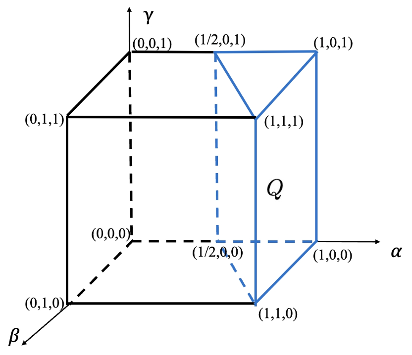
Figure 1: The region of $Q$ (blue triangular prism).

The closedness of $\mathcal{A}$ is not obvious, we thereby have the following Lemma.

Lemma 2.1.

Let $m\geq 0$ and $(\alpha,\beta,\gamma)\in Q$, $\mathcal{H}$ and $\mathcal{A}$ be defined by (2.1) and (2.2), respectively. Then ${\mathcal{A}}$ is closed.

Proof.

Assume that there exists $U_{n}=(u_{n},v_{n},\theta_{n},q_{n})^{\top}\in\mathcal{D}(\cal A)$ such that $U_{n}\to U_{0}:=(u_{0},v_{0},\theta_{0},q_{0})^{\top}$ in $\mathcal{H}$, $\mathcal{A}U_{n}\to W:=(w_{1},w_{2},w_{3},w_{4})^{\top}$ in $\mathcal{H}$, i.e.,

$$\left(\begin{array}[]{c}v_{n}\\ -(I+mA^{\gamma})^{-1}(\sigma Au_{n}-A^{\alpha}\theta_{n})\\ -A^{\alpha}v_{n}+A^{\frac{\beta}{2}}q_{n}\\ \displaystyle{1\over\tau}(-q_{n}-A^{\frac{\beta}{2}}\theta_{n})\end{array}\right)\to\left(\begin{array}[]{c}w_{1}\\ w_{2}\\ w_{3}\\ w_{4}\end{array}\right),\quad\text{in }\mathcal{D}(A^{\frac{1}{2}})\times\mathcal{D}(A^{\frac{\gamma}{2}})\times H\times H.$$

It suffices to show $U_{0}\in\mathcal{D}(\cal A)$ and $\mathcal{A}U_{0}=W$.

By the assumption we have $v_{n}\to w_{1}$ in $\mathcal{D}(A^{1/2})$, $v_{n}\to v_{0}$ in $\mathcal{D}(A^{\gamma/2})$, then $v_{0}=w_{1}$.

Since $U_{n}\in\mathcal{D}(\cal A)$, which implies $-q_{n}-A^{\beta/2}\theta_{n}\in H$, then $B_{n}:=-A^{-\beta/2}q_{n}-\theta_{n}\in\mathcal{D}(A^{\beta/2})$. Recalling that $A$ is a self-adjoint, positive definite operator on $H$, $q_{n}\to q_{0}$ in $H$, therefore, $A^{-\beta/2}q_{n}\to A^{-\beta/2}q_{0}$ in $H$, which together with $\theta_{n}\to\theta_{0}$ in $H$ implies

$$B_{n}\to-A^{-\beta/2}q_{0}-\theta_{0}\quad\text{in }H.$$

Moreover, by the assumption we have $A^{\beta/2}B_{n}\to\tau w_{4}$ in $H$. Note that $A^{\beta/2}$ is closed, we get $-q_{0}-A^{\frac{\beta}{2}}\theta_{0}=\tau w_{4}$.

By a similar argument as above, we can prove that $-A^{\alpha}v_{0}+A^{\frac{\beta}{2}}q_{0}=w_{3}$ and $-(I+mA^{\gamma})^{-1}(\sigma Au_{0}-A^{\alpha}\theta_{0})=w_{2}$. In conclusion,

$$\left(\begin{array}[]{c}v_{0}\\ -(I+mA^{\gamma})^{-1}(\sigma Au_{0}-A^{\alpha}\theta_{0})\\ -A^{\alpha}v_{0}+A^{\frac{\beta}{2}}q_{0}\\ \displaystyle{1\over\tau}(-q_{0}-A^{\frac{\beta}{2}}\theta_{0})\end{array}\right)=\left(\begin{array}[]{c}w_{1}\\ w_{2}\\ w_{3}\\ w_{4}\end{array}\right)\in\mathcal{H},$$

which further implies that $U_{0}\in\mathcal{D}(\mathcal{A})$. The proof is complete. ∎

The well-posedness of the system (2.3) is stated as follows.

Theorem 2.2.

Let $m>0$ and $(\alpha,\beta,\gamma)\in Q$, $\mathcal{H}$ and $\mathcal{A}$ be defined by (2.1) and (2.2), respectively. Then $\mathcal{A}$ generates a $C_{0}$-semigroup $(T(t))_{t\geq 0}$ of contractions on $\mathcal{H}$.

Proof.

We have shown in Lemma 2.1 that $\mathcal{A}$ is a closed operator. Note that $\mathcal{D}(\mathcal{A})\supseteq{\cal D}_{0}:=\mathcal{D}(A^{1-\frac{\gamma}{2}})\times\mathcal{D}(A^{\alpha})\times\mathcal{D}(A^{\alpha-\frac{\gamma}{2}})\times\mathcal{D}(A^{\frac{\beta}{2}})$, and ${{\overline{{\cal D}_{0}}}=\mathcal{H}}$, thus $\mathcal{A}$ is densely defined on $\mathcal{H}$. Furthermore, for any vector $U=(u,v,\theta,q)^{\top}\in\mathcal{D}(\mathcal{A})$, we have

$${\cal R}e\langle\mathcal{A}U,U\rangle_{\mathcal{H}}=-\|q\|^{2},$$ (2.4)

indicating that $\mathcal{A}$ is dissipative. By direct calculation, one gets $\mathcal{A}^{*}:\mathcal{D}(\mathcal{A}^{*})\to\mathcal{H}$ is dissipative as well. By [15, Corollary I.4.4], $\mathcal{A}$ is the generator of a $C_{0}$-semigroup $(T(t))_{t\geq 0}$ of contraction on $\mathcal{H}$. ∎

We now show that 0 is the unique spectral point of $\mathcal{A}$ on the imaginary axis when $\alpha>\frac{\beta+1}{2}$.

Theorem 2.3.

Let $m>0$ and $(\alpha,\beta,\gamma)\in Q$, $\mathcal{H}$ and $\mathcal{A}$ be defined by (2.1) and (2.2), respectively. Then $\sigma(\mathcal{A})\cap i\mathbb{R}=\{0\}$.

Proof.

We first claim that ${\mathcal{A}}$ is not surjective, then $0\in\sigma(\mathcal{A})$. Otherwise, for any $G:=(g_{1},g_{2},g_{3},g_{4})^{\top}\in\mathcal{H}$, there exists $U=(u,v,\theta,q)^{\top}\in\mathcal{D}(\mathcal{A})$ such that $\mathcal{A}U=G$. Solving the equation gives

$$v=g_{1},\quad\theta=-A^{-\frac{\beta}{2}}(\tau g_{4}+A^{-\frac{\beta}{2}}(g_{3}+A^{\alpha}g_{1})),\quad q=A^{-\frac{\beta}{2}}(g_{3}+A^{\alpha}g_{1}),$$

and

$$u=\sigma^{-1}A^{-1}(A^{\alpha}\theta-(I+mA^{\gamma})g_{2}).$$

However, from the equation of $q$, one has $A^{\alpha-\frac{\beta}{2}}g_{1}\in\mathcal{H}$, which is in contradiction with the arbitrariness of $g_{1}\in\mathcal{D}(A^{\frac{1}{2}})$. Therefore, ${\mathcal{A}}$ is not surjective.

We proceed to prove $i\mathbb{R}\backslash\{0\}\subseteq\rho(\mathcal{A})$. Suppose that there exists a $\lambda\in\mathbb{R}\backslash\{0\}$ such that $i\lambda\in\sigma(\mathcal{A})$. Then there exists a sequence $U_{n}=(u_{n},v_{n},\theta_{n},q_{n})^{\top}\subseteq\mathcal{D}(\mathcal{A})$ with

$$\|U_{n}\|_{\mathcal{H}}=1,\;\;\forall\;n\in\mathbb{N},$$ (2.5)

such that

$$\|(i\lambda I-\mathcal{A})U_{n}\|_{\mathcal{H}}=o(1),\quad n\to\infty,$$

i.e.,

$$i\lambda A^{\frac{1}{2}}u_{n}-A^{\frac{1}{2}}v_{n}=o(1)\quad\mbox{in }\;H,$$ (2.6)

$$A^{-\frac{\gamma}{2}}\left(i\lambda v_{n}+i\lambda mA^{\gamma}v_{n}+\sigma Au_{n}-A^{\alpha}\theta_{n}\right)=o(1)\quad\mbox{in }\;H,$$ (2.7)

$$i\lambda\theta_{n}+A^{\alpha}v_{n}-A^{\frac{\beta}{2}}q_{n}=o(1)\quad\mbox{in }\;H,$$ (2.8)

$$i\lambda\tau q_{n}+q_{n}+A^{\frac{\beta}{2}}\theta_{n}=o(1)\quad\mbox{in }\;H.$$ (2.9)

By a direct calculation we get

$$\|q_{n}\|^{2}=-{\cal R}e\langle\mathcal{A}{U_{n}},{U_{n}}\rangle_{\mathcal{H}}={\cal R}e\langle(i\lambda I-\mathcal{A})U_{n},U_{n}\rangle_{\mathcal{H}}=o(1).$$ (2.10)

Combining (2.9) and (2.10), one has

$$\|A^{\frac{\beta}{2}}\theta_{n}\|=o(1),\;\;\|\theta_{n}\|=o(1).$$ (2.11)

Note that $\alpha>\frac{\beta+1}{2}$, we obtain the following identity from (2.8):

$$i\lambda A^{\frac{\gamma}{2}-\alpha}\theta_{n}+A^{\frac{\gamma}{2}}v_{n}-A^{\frac{\beta+\gamma}{2}-\alpha}q_{n}=o(1).$$ (2.12)

We deduce from (2.10)-(2.12) that

$$\|A^{\frac{\gamma}{2}}v_{n}\|=o(1),\;\;\|v_{n}\|=o(1).$$ (2.13)

Taking the inner product of (2.8) with $\theta_{n}$ yields

$$i\lambda\|\theta_{n}\|^{2}+(A^{\alpha}v_{n},\theta_{n})-(A^{\frac{\beta}{2}}q_{n},\theta_{n})=o(1){.}$$

It is easy to see from (2.10) and (2.11) and the above that

$$(A^{\alpha}\theta_{n},v_{n})=o(1).$$ (2.14)

Taking the inner product of (2.7) with $A^{\frac{\gamma}{2}}v_{n}$ on $H$, combining with (2.6), we get

$$i\lambda\|v_{n}\|^{2}+i\lambda m\|A^{\frac{\gamma}{2}}v_{n}\|^{2}-i\lambda\sigma\|A^{\frac{1}{2}}u_{n}\|^{2}-(A^{\alpha}\theta_{n},v_{n})=o(1),$$

which together with (2.13) and (2.14), yields

$$\|A^{\frac{1}{2}}u_{n}\|=o(1).$$ (2.15)

Therefore, we arrive at the contradiction that $\|U_{n}\|_{\mathcal{H}}=o(1)$ according to (2.10),(2.11), (2.13), and (2.15). The proof is complete. ∎

By the same argument as above, we can prove the well-posedness of system (1.1) without inertial term, i.e., when $m=0.$

Theorem 2.4.

Let $\mathcal{H}$ and $\mathcal{A}$ be defined by (2.1) and (2.2) with $m=0$ and $(\alpha,\beta)\in Q^{\ast}$, where the region $Q^{*}$ is defined by (see Figure 2)

$$Q^{*}:=\Big{\{}(\alpha,\beta)\in[0,1]\times[0,1]\Big{|}\alpha>\frac{\beta+1}{2}\Big{\}}.$$

Then $\mathcal{A}$ generates a $C_{0}$-semigroup $(T(t))_{t\geq 0}$ of contractions on $\mathcal{H}$. Furthermore, $\sigma(\mathcal{A})\cap i\mathbb{R}=\{0\}$.

In this paper, we explore the long-time behavior of the solution $T(\cdot)U_{0}$ of system (2.3) for initial values $U_{0}$ belonging to $\mathcal{D}({\mathcal{A}})\cap\mathcal{R}(\mathcal{A})$. Note that since $\mathcal{A}$ generates a $C_{0}$-semigroup $(T(t))_{t\geq 0}$ of contractions on $\mathcal{H}$, $-\mathcal{A}$ is a sectorial operator and thereby $\mathcal{R}({\mathcal{A}}^{s}(I-{\mathcal{A}})^{-(s+t)})=\mathcal{R}({\mathcal{A}}^{s})\cap\mathcal{D}({\mathcal{A}}^{t})$ for $s,t\geq 0$ by [3, Proposition 3.10]. The main results are stated as follows.

Theorem 2.5.

Let $m>0$ and $(\alpha,\beta,\gamma)\in Q$, $\mathcal{H}$ and $\mathcal{A}$ be defined by (2.1) and (2.2), respectively. Suppose that $(T(t))_{t\geq 0}$ is the $C_{0}$-semigroup of contractions generated by ${\mathcal{A}}$. Then as $t\to\infty,$

$$\big{\|}T(t){\mathcal{A}}(I-{\mathcal{A}})^{-\big{(}1+\frac{2(2\alpha-\beta-\gamma)}{2\alpha-\gamma}\big{)}}\big{\|}=O(t^{-1}),$$ (2.16)

and

$$\big{\|}T(t){\mathcal{A}}(I-{\mathcal{A}})^{-2}\big{\|}=O(t^{-\frac{1}{a}}),\quad a=\max\Big{\{}1,\;\frac{2(2\alpha-\beta-\gamma)}{2\alpha-\gamma}\Big{\}}.$$ (2.17)

Moreover, the decay rate of (2.17) is sharp if $\alpha\geq\beta+\frac{\gamma}{2}$.

Remark 2.6.

It is obvious that (2.17) is a consequence of (2.16) if $\alpha<\beta+\frac{\gamma}{2}$, the optimal decay rate of (2.17) in this case is unclear.

The following theorem gives the stability of the abstract coupled thermoelastic system (1.1) without inertial term.

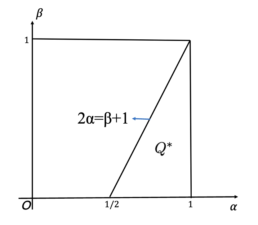
Figure 2: The region of $Q^{*}$.

Theorem 2.7.

Let $m=0$ and $(\alpha,\beta)\in Q^{*}$, $\mathcal{H}$ and $\mathcal{A}$ be defined by (2.1) and (2.2), respectively. Suppose that $(T(t))_{t\geq 0}$ is the $C_{0}$-semigroup of contractions generated by $\mathcal{A}$. Then

$$\big{\|}T(t){\mathcal{A}}(I-{\mathcal{A}})^{-2}\big{\|}=O(t^{-\frac{\alpha}{2\alpha-\beta}}),\quad t\to\infty.$$ (2.18)

Moreover, the decay rate of (2.18) is sharp.

We shall prove Theorems 2.5 and 2.7 by estimating the norm of the corresponding resolvent operator along the imaginary axis, especially at zero and infinity on the imaginary axis. Our proof is based on the following result on frequency characteristics for polynomial-stable semigroup.

Lemma 2.8.

([3, Theorem 8.4]) Let $(T(t))_{t\geq 0}$ be a bounded $C_{0}$-semigroup on a Hilbert space $\mathcal{H}$ with generator $\mathcal{A}$. Assume that $\sigma(\mathcal{A})\cap i\mathbb{R}=\{0\}$ and that there exist $l\geq 1$, $k>0$ such that

$$\big{\|}(isI-\mathcal{A})^{-1}\big{\|}=\left\{\begin{aligned} &O(|s|^{-l}),&s\to 0,\\ &O(|s|^{k}),&|s|\to\infty.\end{aligned}\right.$$ (2.19)

Then

$$\big{\|}T(t)\mathcal{A}^{l}(I-\mathcal{A})^{-(l+k)}\big{\|}=O(t^{-1}),\;t\to\infty,$$

and

$$\big{\|}T(t)\mathcal{A}(I-\mathcal{A})^{-2}\big{\|}=O(t^{-\frac{1}{a}}),\;t\to\infty,$$ (2.20)

where $a=\max\{l,k\}$.

Conversely, if (2.20) holds for some $a>0$, then (2.19) holds for $l=\max\{a,1\}$ and $k=a$.

At the end of this section, we present the following interpolation lemma, which will be utilized in subsequent sections.

Lemma 2.9.

Let $A\,:\,{\cal D}(A)\subseteq H$ be self-adjoint and positive definite, $r,\;p\;,q\in\mathbb{R}$. Then

$$\|A^{p}x\|\leq\|A^{q}x\|^{p-r\over q-r}\|A^{r}x\|^{q-p\over q-r},\quad\forall\;r\leq p\leq q,\;x\in{\cal D}(A^{q}).$$ (2.21)

3 Stability of system with inertial term (Proof of Theorem 2.5)

In this section, we focus on analyzing the polynomial stability of the system (1.1), considering $m>0$, specifically aiming to prove Theorem 2.5. According to Lemma 2.8, it is sufficient to show that for $k=\frac{2(2\alpha-\beta-\gamma)}{2\alpha-\gamma},\;l=1$, the following holds:

$$\begin{array}[]{ll}&\|s(isI-\mathcal{A})^{-1}\|=O(1),\;\;s\to 0,\\ &\|\lambda^{-k}(i\lambda I-\mathcal{A})^{-1}\|=O(1),\;\;\lambda\to\infty.\end{array}$$ (3.3)

If (3.3) fails, there exists a sequence $(\eta_{n},\lambda_{n},U_{1,n},U_{2,n})_{n\geq 1}$, where $\eta_{n}:=s_{n}^{-1},\lambda_{n}\in{\mathbb{R}},U_{j,n}:=(u_{j,n},{v}_{j,n},\theta_{j,n},\,q_{j,n})^{\top}\in\mathcal{D}({\cal A}),j=1,2$ satisfying

$$\|U_{j,n}\|_{\cal H}=\big{\|}(u_{j,n},{v}_{j,n},\theta_{j,n},q_{j,n})^{\top}\big{\|}_{\cal H}=1,\;j=1,2,$$ (3.4)

such that as $n\to\infty,\eta_{n},\lambda_{n}\to\infty$, and

$$(iI-\eta_{n}{\mathcal{A}})U_{1,n}=o(1),\;\;\;\;\qquad\lambda_{n}^{k}\big{(}i\,\lambda_{n}I-{\mathcal{A}}\big{)}U_{2,n}=o(1)\;\mbox{ in }\;{\cal H}.$$ (3.5)

Equivalently, we have

$$iA^{\frac{1}{2}}u_{1,n}-\eta_{n}A^{\frac{1}{2}}v_{1,n}=o(1)\quad\;\mbox{ in }\;H,$$ (3.6)

$$A^{-\frac{\gamma}{2}}\left(iv_{1,n}+imA^{\gamma}v_{1,n}+\sigma\eta_{n}Au_{1,n}-\eta_{n}A^{\alpha}\theta_{1,n}\right)=o(1)\quad\;\mbox{ in }\;H,$$ (3.7)

$$i\theta_{1,n}-\eta_{n}A^{\frac{\beta}{2}}q_{1,n}+\eta_{n}A^{\alpha}v_{1,n}=o(1)\quad\;\mbox{ in }\;H,$$ (3.8)

$$i\tau q_{1,n}+\eta_{n}q_{1,n}+\eta_{n}A^{\frac{\beta}{2}}\theta_{1,n}=o(1)\quad\;\mbox{ in }\;H.$$ (3.9)

and

$$\lambda_{n}^{k}(i\lambda_{n}A^{\frac{1}{2}}u_{2,n}-A^{\frac{1}{2}}v_{2,n})=o(1)\quad\;\mbox{ in }\;H,$$ (3.10)

$$\lambda_{n}^{k}A^{-\frac{\gamma}{2}}\left(i\lambda_{n}v_{2,n}+i\lambda_{n}mA^{\gamma}v_{2,n}+\sigma Au_{2,n}-A^{\alpha}\theta_{2,n}\right)=o(1)\quad\;\mbox{ in }\;H,$$ (3.11)

$$\lambda_{n}^{k}(i\lambda_{n}\theta_{2,n}-A^{\frac{\beta}{2}}q_{2,n}+A^{\alpha}v_{2,n})=o(1)\quad\;\mbox{ in }\;H,$$ (3.12)

$$\lambda_{n}^{k}(i\lambda_{n}\tau q_{2,n}+q_{2,n}+A^{\frac{\beta}{2}}\theta_{2,n})=o(1)\quad\;\mbox{ in }\;H.$$ (3.13)

We shall prove $\|U_{j,n}\|=o(1),\;j=1,2$, which contradicts to the assumption (3.4). The proof is structured into two steps.

Step 1. We claim that $\|U_{1,n}\|=o(1).$

By (2.4) and the first identity of (3.5), it is easy to see

$$\|q_{1,n}\|=\eta_{n}^{-\frac{1}{2}}o(1).$$ (3.14)

According to (3.9) and (3.14), we get

$$\|A^{\frac{\beta}{2}}\theta_{1,n}\|=\eta_{n}^{-\frac{1}{2}}o(1).$$ (3.15)

Therefore,

$$\|\theta_{1,n}\|=o(1).$$ (3.16)

Combining $\alpha>\frac{1}{2}$ and $\eqref{unitnorm}$, one has $\|A^{-\alpha+\gamma}v_{1,n}\|$ is bounded. Thus, taking the inner product of (3.8) with $\eta^{-1}_{n}A^{-\alpha+\gamma}v_{1,n}$, we have

$$i\eta^{-1}_{n}(\theta_{1,n},A^{-\alpha+\gamma}v_{1,n})-(A^{\frac{\beta}{2}}q_{1,n},A^{-\alpha+\gamma}v_{1,n})+\|A^{\frac{\gamma}{2}}v_{1,n}\|^{2}=o(1).$$ (3.17)

The first term of (3.17) tends to 0 because of (3.16) and the boundedness of $\|A^{-\alpha+\gamma}v_{1,n}\|$. The second term of (3.17) tends to 0 because of (3.14) and $-\alpha+\frac{\beta}{2}+\gamma<\frac{\gamma}{2}$. Therefore,

$$\|A^{\frac{\gamma}{2}}v_{1,n}\|=o(1),\;\;\mbox{and then }\;\|v_{1,n}\|=o(1).$$ (3.18)

From (3.8), we see $i\eta_{n}^{-\frac{1}{2}}A^{-\frac{\beta}{2}}\theta_{1,n}-\eta_{n}^{\frac{1}{2}}q_{1,n}+\eta_{n}^{\frac{1}{2}}A^{\alpha-\frac{\beta}{2}}v_{1,n}=o(1).$ Thus, by (3.14) and (3.16), we get

$$\|\eta_{n}^{\frac{1}{2}}A^{\alpha-\frac{\beta}{2}}v_{1,n}\|=o(1).$$ (3.19)

Taking the inner product of (3.7) with $A^{\frac{\gamma}{2}}v_{1,n}$ on $H$ yields

$$i\|v_{1,n}\|^{2}+im\|A^{\frac{\gamma}{2}}v_{1,n}\|^{2}+(\sigma A^{\frac{1}{2}}u_{1,n},\eta_{n}A^{\frac{1}{2}}v_{1,n})-(\eta_{n}A^{\alpha}\theta_{1,n},v_{1,n})=o(1).$$ (3.20)

By (3.6) and (3.20), we get

$$i\|v_{1,n}\|^{2}+im\|A^{\frac{\gamma}{2}}v_{1,n}\|^{2}-i\sigma\|A^{\frac{1}{2}}u_{1,n}\|^{2}-(\eta_{n}A^{\alpha}\theta_{1,n},v_{1,n})=o(1).$$ (3.21)

Recalling (3.15) and (3.19), one has

$$(\eta_{n}A^{\alpha}\theta_{1,n},v_{1,n})\leq\|\eta_{n}^{\frac{1}{2}}A^{\frac{\beta}{2}}\theta_{1,n}\|\|\eta_{n}^{\frac{1}{2}}A^{\alpha-\frac{\beta}{2}}v_{1,n}\|=o(1).$$

Combining this, (3.18) and (3.21), we obtain

$$\|A^{\frac{1}{2}}u_{1,n}\|=o(1).$$ (3.22)

In summary, by (3.14), (3.16), (3.18) and (3.22), we conclude $\|U_{1,n}\|_{\mathcal{H}}=\|(u_{1,n},v_{1,n},\theta_{1,n},q_{1,n})\|_{\mathcal{H}}=o(1)$.

Step 2. We claim that $\|U_{2,n}\|_{\mathcal{H}}=o(1)$.

By (2.4) and the second identity of (3.5), it is easy to see

$$\|q_{2,n}\|=\lambda_{n}^{-\frac{k}{2}}o(1).$$ (3.23)

According to (3.13) and (3.23), we get

$$\|A^{\frac{\beta}{2}}\theta_{2,n}\|=\lambda_{n}^{1-\frac{k}{2}}o(1).$$ (3.24)

Since $\alpha>\frac{\beta+1}{2}$, (3.12) implies

$$i\lambda_{n}A^{-\alpha+\frac{\gamma}{2}}\theta_{2,n}-A^{-\alpha+\frac{\gamma}{2}+\frac{\beta}{2}}q_{2,n}+A^{\frac{\gamma}{2}}v_{2,n}=\lambda_{n}^{-k}o(1).$$

Recalling (3.4) and (3.23), we obtain from the above that

$$\|\lambda_{n}A^{-\alpha+\frac{\gamma}{2}}\theta_{2,n}\|=O(1).$$ (3.25)

By interpolation we deduce from (3.24) and (3.25) that

$$\left\|\theta_{2,n}\right\|\leq\|A^{\frac{\beta}{2}}\theta_{2,n}\|^{\frac{2\alpha-\gamma}{2\alpha+\beta-\gamma}}\|A^{-\alpha+\frac{\gamma}{2}}\theta_{2,n}\|^{\frac{\beta}{2\alpha+\beta-\gamma}}=o(1).$$ (3.26)

Taking the inner product of (3.11) with $\lambda_{n}^{-k}A^{-\alpha+\frac{\gamma}{2}}\theta_{2,n}$, (3.12) with $\lambda_{n}^{-k}A^{-\alpha}(I+mA^{\gamma})v_{2,n}$ and then adding them, we get

$${{\cal R}e}(\sigma\theta_{2,n},\,A^{1-\alpha}u_{2,n})-{{\cal R}e}{(q_{2,n},\,A^{\frac{\beta}{2}-\alpha}(I+mA^{\gamma})v_{2,n})}-\|\theta_{2,n}\|^{2}+\|v_{2,n}\|^{2}+m\|A^{\frac{\gamma}{2}}v_{2,n}\|^{2}=\lambda_{n}^{-k}o(1).$$ (3.27)

The first two terms in (3.27) tend to 0 because of (3.23), (3.26) and the boundedness of $\|A^{\frac{1}{2}}u_{2,n}\|$ and $\|A^{\gamma\over 2}v_{2,n}\|$. These, along with (3.26) and (3.27), imply

$$\|v_{2,n}\|,~{}~{}\|A^{\frac{\gamma}{2}}v_{2,n}\|=o(1).$$ (3.28)

One can deduce from (3.11) that

$$iA^{-\frac{1}{2}}v_{2,n}+imA^{\gamma-\frac{1}{2}}v_{2,n}+\sigma\lambda_{n}^{-1}A^{\frac{1}{2}}u_{2,n}-\lambda_{n}^{-1}A^{\alpha-\frac{1}{2}}\theta_{2,n}=\lambda_{n}^{-k-1}o(1),$$

which along with (3.28) and the boundedness of $\|A^{\frac{1}{2}}u_{2,n}\|$, yields

$$\|\lambda_{n}^{-1}A^{\alpha-\frac{1}{2}}\theta_{2,n}\|=o(1).$$ (3.29)

Now, taking the inner product of (3.11) with ${\lambda_{n}^{-k}}A^{\frac{\gamma}{2}}u_{2,n}$ on $H$, along with (3.10), one has

$$-\|v_{2,n}\|^{2}-m\|A^{\frac{\gamma}{2}}v_{2,n}\|^{2}+\sigma\|A^{\frac{1}{2}}u_{2,n}\|^{2}-(A^{\alpha}\theta_{2,n},u_{2,n})=o(1).$$ (3.30)

Note that by (3.10) and (3.29), we have

$$\begin{array}[]{ll}(A^{\alpha}\theta_{2,n},\,u_{2,n})&=i(\lambda_{n}^{-1}A^{\alpha}\theta_{2,n},\,v_{2,n})+o(1)\\ &=i(A^{\frac{\beta}{2}}\theta_{2,n},\,\lambda_{n}^{-1}A^{\alpha-\frac{\beta}{2}}v_{2,n})+o(1).\end{array}$$ (3.31)

Furthermore, by $\eqref{s3+}$, we see

$$\lambda_{n}^{-1}A^{\alpha-\frac{\beta}{2}}v_{2,n}=-{\color[rgb]{1.00,0.00,0.00}i}A^{-\frac{\beta}{2}}\theta_{2,n}+\lambda_{n}^{-1}q_{2,n}+\lambda_{n}^{-k-1}o(1){.}$$ (3.32)

Substituting (3.32) into (3.31) yields

$$(A^{\alpha}\theta_{2,n},\,u_{2,n})=-\|\theta_{2,n}\|^{2}+i(\lambda_{n}^{-1}A^{\frac{\beta}{2}}\theta_{2,n},\,q_{2,n})=o(1),$$

where we use (3.23), (3.24) and (3.26). Combining this, (3.28) and (3.30), we obtain

$$\|A^{\frac{1}{2}}u_{2,n}\|={o(1)}.$$ (3.33)

Recalling (3.23), (3.26), (3.28) and (3.33), we get $\|U_{2,n}\|_{\mathcal{H}}=o(1)$, which contradicts (3.4). Therefore, by the above two steps, we have proved that the assumption (3.3) holds with $k=\frac{2(2\alpha-\beta-\gamma)}{2\alpha-\gamma},\;l=1$. As a result, thanks to Lemma 2.8, the semigroup $T(t)$ satisfies (2.16)-(2.17) when $t\to\infty$.

At the end of this section, we show that the decay order is sharp if $\alpha\geq\beta+\frac{\gamma}{2}$, i.e., $k\geq 1$ by analyzing the eigenvalues. Noticing that $A$ is a self-adjoint, positive definite operator with compact resolvent. Thus, there exists a sequence of eigenvalues $\{\mu_{n}\}_{n\geq 1}$ of $A$ such that

$$0<\mu_{1}\leq\mu_{2}\leq\cdots\leq\mu_{n}\leq\cdots,~{}~{}\qquad\lim_{n\to\infty}\mu_{n}=\infty.$$

Using the same method in [6], we know that the eigenvalues $\lambda_{n}$ of operator ${\cal A}$ satisfy the following quartic equation:

$$(\mu_{n}^{\gamma}+1)\lambda_{n}^{4}+(\mu_{n}^{\gamma}+1)\lambda_{n}^{3}+(\mu_{n}^{2\alpha}+\mu_{n}^{\beta+\gamma}+2\mu_{n}+\mu_{n}^{\beta})\lambda_{n}^{2}+(\mu_{n}^{2\alpha}+2\mu_{n})\lambda_{n}+2\mu_{n}^{1+\beta}=0,$$ (3.34)

where $\mu_{n},\;n=1,2,\cdots$ are the eigenvalues of the operator $A$. By [6, Section 5.1], we get that the solutions to (3.34) when $(\alpha,\beta,\gamma)\in Q$ are as follows:

$$\lambda_{1,n} =-\frac{1}{2}\mu_{n}^{-2\alpha+\beta+\gamma}(1+o(1))+i\mu_{n}^{\alpha-\frac{\gamma}{2}}(1+o(1)),$$

$$\lambda_{2,n} =-\frac{1}{2}\mu_{n}^{-2\alpha+\beta+\gamma}(1+o(1))-i\mu_{n}^{\alpha-\frac{\gamma}{2}}(1+o(1)),$$

$$\lambda_{3,n} =-2\mu_{n}^{-2\alpha+\beta+1}(1+o(1)),$$

$$\lambda_{4,n} =-1(1+o(1)).$$

It is easy to see from $\lambda_{1,n}$ and $\lambda_{2,n}$ that

$$|{\cal R}e\lambda_{i,n}|=\frac{1}{2}|{\cal I}m\lambda_{i,n}|^{-{k}},\quad\;\mbox{ when }\;(\alpha,\;\beta,\;\gamma)\in Q,\;i=1,2.$$ (3.35)

The following proposition gives the sharpness of the decay rate.

Proposition 3.1.

Let the conditions in Theorem 2.5 hold. Suppose $\alpha\geq\beta+\frac{\gamma}{2}$. Then the decay rate in (2.17) is sharp.

Proof.

By the proof of Theorem 2.5, estimation (2.19) in Lemma 2.8 holds with $k=\frac{2(2\alpha-\beta-\gamma)}{2\alpha-\gamma},\;l=1$. If $\alpha\geq\beta+\frac{\gamma}{2}$, then $k\geq 1$. Consequently, we have

$$\|T(t){\mathcal{A}}(I-{\mathcal{A}})^{-2}\|=O(t^{-\frac{1}{k}}),\;t\to\infty.$$

We only prove the case when $k>1$, the case when $k=1$ is similar. If the decay rate can be improved, in other words, there exists $\varepsilon>0$ small enough such that $k-\varepsilon>1$ and $\|T(t){\mathcal{A}}(I-{\mathcal{A}})^{-2}\|=O(t^{-\frac{1}{k-\varepsilon}})$, then by Lemma 2.8, one has

$$\|(i\lambda I-{\mathcal{A}})^{-1}\|=\left\{\begin{aligned} &O(|\lambda|^{-k+\varepsilon}),&\lambda\to 0,\\ &O(|\lambda|^{k-\varepsilon}),&|\lambda|\to\infty.\end{aligned}\right.$$

In particular, there exists a constant $C>1$ such that

$$\|(i\lambda I-{\mathcal{A}})^{-1}\|\leq C|\lambda|^{k-\varepsilon},\;\;|\lambda|\to\infty.$$ (3.36)

Let $S_{\lambda}:=\big{\{}r+i\lambda\,\big{|}\,|r|\leq\frac{1}{2C|\lambda|^{k-\varepsilon}},\;r,\;\lambda\in{\mathbb{R}\backslash\{0\}}\big{\}}$, then for any $s\in S_{\lambda}$,

$$\|(sI-{\mathcal{A}})^{-1}\| =\|(i\lambda I-{\mathcal{A}})^{-1}(I+r(i\lambda I-{\mathcal{A}})^{-1})^{-1}\|$$

$$\leq\|(i\lambda I-{\mathcal{A}})^{-1}\|\frac{1}{1-\|r(i\lambda I-{\mathcal{A}})^{-1}\|}$$

$$\leq 2\|(i\lambda I-\mathcal{A})^{-1}\|$$

$$\leq 2C|\lambda|^{k-\varepsilon},\;\;\;|\lambda|\to\infty,$$

which implies that $S_{\lambda}\subseteq\rho({\mathcal{A}})$ for $|\lambda|$ big enough.

On the other hand, recalling that there exists a sequence $(\lambda_{n})_{n\geq 1}\subseteq\sigma({\mathcal{A}}),\;|\lambda_{n}|\to\infty$ such that (3.35) holds. For the constant $C$ in (3.36) and an arbitrary positive constant $\varepsilon$, we choose $\lambda_{n}$ such that $|{\cal I}m\lambda_{n}|^{-\varepsilon}\leq\frac{1}{C}$, then

$$|{\cal R}e\lambda_{n}|=\frac{1}{2}|{\cal I}m\lambda_{n}|^{-{k}}\leq\frac{1}{2C|{\cal I}m\lambda_{n}|^{k-\varepsilon}}.$$

Thus, $\lambda_{n}\in S_{\lambda_{n}}$ which contradicts $\lambda_{n}\in\sigma({\mathcal{A}})$. ∎

4 Stability of system without inertial term (Proof of Theorem 2.7)

In this section, we shall analyze the polynomial stability of system (1.1) without inertial term, i.e., prove Theorem 2.7. By Lemma 2.8, it is sufficient to show that (2.19) holds with $k=\frac{2\alpha-\beta}{\alpha},\;l=1$. Similar to the argument in Section 3, we still prove this theorem by contradiction. Suppose (2.19) fails, then there at least exists a sequence $\{\eta_{n},\lambda_{n},U_{1,n},U_{2,n}\}_{n=1}^{\infty}\subseteq{\mathbb{R}}^{2}\times\mathcal{D}({\cal A})^{2}$ such that (3.4)-(3.5) hold with $m=0$. In other words, we have

$$iA^{\frac{1}{2}}u_{1,n}-\eta_{n}A^{\frac{1}{2}}v_{1,n}=o(1)\quad\;\mbox{ in }\;H,$$ (4.1)

$$iv_{1,n}+\sigma\eta_{n}Au_{1,n}-\eta_{n}A^{\alpha}\theta_{1,n}=o(1)\quad\;\mbox{ in }\;H,$$ (4.2)

$$i\theta_{1,n}-\eta_{n}A^{\frac{\beta}{2}}q_{1,n}+\eta_{n}A^{\alpha}v_{1,n}=o(1)\quad\;\mbox{ in }\;H,$$ (4.3)

$$i\tau q_{1,n}+\eta_{n}q_{1,n}+\eta_{n}A^{\frac{\beta}{2}}\theta_{1,n}=o(1)\quad\;\mbox{ in }\;H.$$ (4.4)

and

$$\lambda_{n}^{k}(i\lambda_{n}A^{\frac{1}{2}}u_{2,n}-A^{\frac{1}{2}}v_{2,n})=o(1)\quad\;\mbox{ in }\;H,$$ (4.5)

$$\lambda_{n}^{k}\left(i\lambda_{n}v_{2,n}+\sigma Au_{2,n}-A^{\alpha}\theta_{2,n}\right)=o(1)\quad\;\mbox{ in }\;H,$$ (4.6)

$$\lambda_{n}^{k}(i\lambda_{n}\theta_{2,n}-A^{\frac{\beta}{2}}q_{2,n}+A^{\alpha}v_{2,n})=o(1)\quad\;\mbox{ in }\;H,$$ (4.7)

$$\lambda_{n}^{k}(i\lambda_{n}\tau q_{2,n}+q_{2,n}+A^{\frac{\beta}{2}}\theta_{2,n})=o(1)\quad\;\mbox{ in }\;H.$$ (4.8)

We are devoted to showing that $\|U_{j,n}\|_{\mathcal{H}}=o(1),\;j=1,2$, which contradicts the assumption (3.4). We first prove $\|U_{1,n}\|_{\mathcal{H}}=o(1).$ Recalling that $\mathcal{A}$ is dissipative, (3.5) and (4.4), we see

$$\|q_{1,n}\|=\eta_{n}^{-\frac{1}{2}}o(1),\;\;\|A^{\frac{\beta}{2}}\theta_{1,n}\|=\eta_{n}^{-\frac{1}{2}}o(1).$$ (4.9)

Therefore,

$$\|\theta_{1,n}\|=o(1).$$ (4.10)

Taking the inner product of (4.3) with $\eta^{-1}_{n}A^{-\alpha}v_{1,n}$, we have

$$i\eta^{-1}_{n}(\theta_{1,n},A^{-\alpha}v_{1,n})-(A^{\frac{\beta}{2}}q_{1,n},A^{-\alpha}v_{1,n})+\|v_{1,n}\|^{2}=o(1).$$ (4.11)

By Cauchy-Schwarz inequality and (4.9)-(4.11), we get

$$\|v_{1,n}\|=o(1){.}$$ (4.12)

Repeating the proof of (3.19), we can deduce from (4.3) and (4.9) that

$$\|A^{\alpha-\frac{\beta}{2}}v_{1,n}\|=\eta_{n}^{-\frac{1}{2}}o(1).$$ (4.13)

Taking the inner product of (4.2) with $v_{1,n}$ on $H$, along with (4.1), one has

$$i\|v_{1,n}\|^{2}-i\sigma\|A^{\frac{1}{2}}u_{1,n}\|^{2}-(\eta_{n}A^{\alpha}\theta_{1,n},v_{1,n})=o(1).$$ (4.14)

By (4.9) and (4.13), the last term of (4.14) goes to 0 as $n\to\infty$. This together with (4.12) implies

$$\|A^{\frac{1}{2}}u_{1,n}\|=o(1).$$ (4.15)

In summary, by (4.9), (4.10), (4.12) and (4.15), we obtain $\|U_{1,n}\|_{\mathcal{H}}=\|(u_{1,n},v_{1,n},\theta_{1,n},q_{1,n})\|_{\mathcal{H}}=o(1)$.

We proceed to prove $\|U_{2,n}\|_{\mathcal{H}}=o(1)$. We obtain from (2.4) and (4.8) that

$$\|q_{2,n}\|=\lambda_{n}^{-\frac{k}{2}}o(1),\;\;\|A^{\frac{\beta}{2}}\theta_{2,n}\|=\lambda_{n}^{1-\frac{k}{2}}o(1)$$ (4.16)

as in Section 3. Note that $-\alpha+\frac{\beta}{2}<0$, then by (3.4) and (4.7), we get

$$\|A^{-\alpha}\theta_{2,n}\|=\lambda_{n}^{-1}O(1).$$

Combining this and (4.16) yields

$$\left\|\theta_{2,n}\right\|\leq\left\|A^{-\alpha}\theta_{2,n}\right\|^{\frac{\beta}{2\alpha+\beta}}\|A^{\frac{\beta}{2}}\theta_{2,n}\|^{\frac{2\alpha}{2\alpha+\beta}}=o(1).$$ (4.17)

It follows from (4.6) that

$$i\lambda_{n}A^{-\alpha}v_{2,n}+\sigma A^{1-\alpha}u_{2,n}-\theta_{2,n}=\lambda_{n}^{-k}o(1).$$

Since $\alpha>\frac{1}{2}$, combining the above, (3.4) and (4.17), one has

$$\|\lambda_{n}A^{-\alpha}v_{2,n}\|=O(1).$$ (4.18)

Taking the inner product of (4.7) with $\lambda_{n}^{-k}A^{-\alpha}v_{2,n}$ yields

$$(i\lambda_{n}\theta_{2,n},A^{-\alpha}v_{2,n})-(A^{\frac{\beta}{2}-\alpha}q_{2,n},v_{2,n})+\|v_{2,n}\|^{2}=o(1).$$ (4.19)

We see the first term of (4.19) tends to 0 because of (4.17) and (4.18), the second term tends to 0 because of (4.16). Thus,

$$\|v_{2,n}\|=o(1).$$ (4.20)

Moreover, by taking the inner product of (4.6) with $\lambda_{n}^{-k-1}v_{2,n}$, together with (4.5), we get

$$i\|v_{2,n}\|^{2}-i\sigma\|A^{\frac{1}{2}}u_{2,n}\|^{2}-(\theta_{2,n},\lambda_{n}^{-1}A^{\alpha}v_{2,n})=o(1).$$

By (4.7), we have $\lambda_{n}^{-1}A^{\alpha}v_{2,n}=-i\theta_{n}+\lambda_{n}^{-1}A^{\frac{\beta}{2}}q_{2,n}+\lambda_{n}^{-1-k}o(1)$. Substituting this into the above equation yields

$$i\|v_{2,n}\|^{2}-i\sigma\|A^{\frac{1}{2}}u_{2,n}\|^{2}-i\|\theta_{2,n}\|^{2}-(\lambda_{n}^{-1}A^{\frac{\beta}{2}}\theta_{2,n},q_{2,n})=o(1).$$ (4.21)

Therefore, we conclude from (4.16), (4.17), (4.20) and (4.21) that

$$\|A^{\frac{1}{2}}u_{2,n}\|={o(1)}.$$ (4.22)

Recalling (4.16), (4.17), (4.20) and (4.22), we get $\|U_{2,n}\|_{\mathcal{H}}=o(1)$, which contradicts to (3.4). Therefore, the assumption (2.19) holds with $k=\frac{2\alpha-\beta}{\alpha},\;l=1$.

Finally, we shall prove the decay order is sharp by a similar argument as in Section 3. Note that $k=\frac{2\alpha-\beta}{\alpha}\geq 1$ always holds. Suppose $\mu_{n},\;\lambda_{n},\;n=1,2,\cdots$ are the eigenvalues of operators $A$ and ${\cal A}$, respectively. Then we have the following quartic equation using the same method in [6, Section 5],

$$\lambda_{n}^{4}+\lambda_{n}^{3}+(\mu_{n}^{2\alpha}+2\mu_{n}+\mu_{n}^{\beta})\lambda_{n}^{2}+(\mu_{n}^{2\alpha}+2\mu_{n})\lambda_{n}+2\mu_{n}^{1+\beta}=0.$$ (4.23)

The solutions to (4.23) when $(\alpha,\beta)\in Q^{*}$ are the following:

$$\lambda_{1,n} =-\frac{1}{2}\mu_{n}^{\beta-2\alpha}(1+o(1))+i\mu_{n}^{\alpha}(1+o(1)),$$

$$\lambda_{2,n} =-\frac{1}{2}\mu_{n}^{\beta-2\alpha}(1+o(1))-i\mu_{n}^{\alpha}(1+o(1)),$$

$$\lambda_{3,n} =-2\mu_{n}^{-2\alpha+\beta+1}(1+o(1)),$$

$$\lambda_{4,n} =-1(1+o(1)).$$

It is clear that

$$|{\cal R}e\lambda_{i,n}|=\frac{1}{2}|{\cal I}m\lambda_{i,n}|^{-{k}},\quad\;\mbox{ when }\;(\alpha,\beta)\in Q^{*},\;i=1,2.$$ (4.24)

Therefore, by the same argument as Proposition 3.1, one can obtain that the decay rate in (2.18) is sharp.

5 Examples

Assume that $\Omega$ is a bounded open subset of $\mathbb{R}^{n}$ with smooth boundary $\Gamma$. Let $A=\Delta^{2}$ be the bi-Laplace operator on $\Omega$ with domain $\mathcal{D}(A)=\{u\in H^{4}(\Omega)\,|\,u|_{\Gamma}=\Delta u|_{\Gamma}=0\},\;H=L^{2}(\Omega),$ $\alpha=1,\,\beta=0,\,\gamma={1\over 2}$. Then the abstract system (1.1) can be written as follows:

$$\left\{\begin{array}[]{ll}u_{tt}-m\Delta u_{tt}+\sigma\Delta^{2}u-\Delta^{2}\theta=0,&x\in\Omega,t>0,\\ \theta_{t}-q+\Delta^{2}u_{t}=0,&x\in\Omega,t>0,\\ \tau q_{t}+q+\theta=0,&x\in\Omega,t>0,\\ u=\Delta u=\theta=q=0,&x\in\Gamma,t>0,\\ u(0)=u_{0},\;u_{t}(0)=u_{1},\;\theta(0)=\theta_{0},\;q(0)=q_{0},&x\in\Omega.\end{array}\right.$$ (5.1)

By Theorems 2.3, 2.4, 2.5 and 2.7, we obtain that zero belongs to the spectrum of the generator of semigroup associated with (5.1) and the semigroup decays polynomially with optimal order $t^{-{1\over 2}}$ for $m\geq 0$.