Second-Order Identification Capacity of AWGN Channels

Abstract

In this paper, we establish the second-order randomized identification capacity (RID capacity) of the Additive White Gaussian Noise Channel (AWGNC). On the one hand, we obtain a refined version of Hayashi’s theorem to prove the achievability part. On the other, we investigate the relationship between identification and channel resolvability, then we propose a finer quantization method to prove the converse part. Consequently, the second-order RID capacity of the AWGNC has the same form as the second-order transmission capacity. The only difference is that the maximum number of messages in RID scales double exponentially in the blocklength.

I Introduction

With the emergence of IoT applications [1, 2], modern communications in the next-generation wireless network framework (XG) require robust and ultra-reliable low latency information exchange between a large pool of potential smart devices. Numerous XG applications are event-triggered communication systems, such as vehicle-X communication [3, 4, 5], tactile internet [6, 7], industry 4.0, Online sales, etc. The emergence of novel communication tasks, including control systems [8], the automotive domain [9], watermarking [10, 11, 12], recommendation systems [13], and other scenarios requiring quick or small checks, presents new challenges. For many of these problems, signaling a user, rather than transmitting a bulk of data, becomes the main task. As such, the identification approach suggested by Ahlswede and Dueck [14] is more suitable than the transmission scheme as studied by Shannon [15]. Some other possible applications of identification codes have been pointed out in [16, 17].

In identification, receiver-$i$ only cares whether message-$i$ is transmitted. Once receiver-$i$ believes message-$i$ is not sent, it does not attempt to decode that message. In randomized identification, message-$i$ is sent by randomly transmitting a codeword from receiver-$i$’s codebook, and it was proved that the optimal code size scales double exponentially in the block length with vanishing type-I and type-II error rates. Han and Verd$\mathrm{\acute{u}}$ [18] provided a new perspective named channel resolvability to further discuss the identification capacity. Subsequently, Steinberg [19] proposed a nuch more tighter converse bound for the randomized identification capacity. Hayashi [20] extended the previous results to wiretap channels and established the error exponents. Han obtained the identification capacity of the continuous input channels in [21]. The second-order RID capacity of the discrete memoryless channels (DMCs) was demonstrated in [22] which relies on the finiteness assumption of the input alphabet, hence can not apply to continuous input channels directly. Based on constant-weight codes (CWCs) that result from concatenating a CWC initialization with outer linear block codes, Verd$\mathrm{\acute{u}}$ and Wei [23] suggested the first explicit ID code construction.

In the deterministic setup, given a discrete memoryless channel (DMC), the number of messages grows exponentially with the blocklength. R. Ahlswede and Ning Cai determined the deterministic identification capacity (DID capacity) for DMCs [24]. In particular, J$\mathrm{\acute{a}}$J$\mathrm{\acute{a}}$ [25] showed that the deterministic identification (DI) capacity of a binary symmetric channel is $1$ bit per channel use, as one can exhaust the entire input space and assign (almost) all binary $n$-tuples as codewords. Recently, Salariseddigh et al. established the deterministic identification capacity for AWGN channels and AWGN channels with slow and fast fading coefficients [26, 27]. Li et al. [28] proposed the deterministic identification capacity for block memoryless fading channels without CSI.

Figure 1 provides a brief overview of the connections between our work and previous research. We extend the results presented by Watanabe to the continuous input alphabet, specifically, by determining the second-order RID capacity for the AWGNCs.

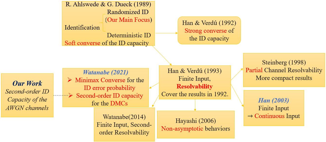
Figure 1: Research status of the Randomized Identification Problems.

In this paper, we derive the second-order RID capacity of the AWGNC. Our contributions are summarized as follows:

1. We propose a refined version of Hayashi’s theorem [20], which results in the achievability part.

2. We propose a finer quantization method than that in [21] to obtain the converse part.

The remainder of this paper is structured as follows. Section II provides the background of the identification and the resolvability. Section III introduces the main results of the paper: the second-order RID capacity of the AWGNC. Finally, we draw conclusions in Section IV. The main differences between our work and the previous studies are provided in Table I.

Notation Conventions: In this paper, the lowercase letters $x$,$y$,$z$,$\cdots$ represent the value of random variables, and uppercase letters $X$,$Y$,$Z$,$\cdots$ represent random variables. The probability distribution of random variable $X$ is specified by a cumulative distribution function (CDF) $F_{X}(x)=\mathrm{Pr}(X\leq x)$, or alternatively, by a probability density function (PDF) $P_{X}(x)$. $X^{n}=(X_{1},...,X_{n})$ and $x^{n}=(x_{1},x_{2},...,x_{n})$ are random vectors of length-$n$ and its realization, respectively. $\mathcal{X}^{n}$ and $\mathcal{Y}^{n}$ represent the $n$th Cartesian product of input alphabet and output alphabet. The $\ell^{2}$-norm of $x^{n}$ is denoted by $||x^{n}||$. A probability distribution $P_{X^{n}}$ is called an $M$-type, if for any integer $M>0$ and every $x^{n}\in\mathcal{X}^{n}$,

$$P_{X^{n}}(x^{n})\in\{0,\frac{1}{M},\frac{2}{M},\cdots,1\}.$$

The variational distance between two probability distributions $P_{X_{1}}$ and $P_{X_{2}}$ defined on the same measurable space $(\Omega,\mathcal{F})$ is $d(P_{X_{1}},P_{X_{2}})=2\sup_{E}|P_{X_{1}}(E)-P_{X_{2}}(E)|$. Denote $\mathcal{P}(\mathcal{X}^{n})$ the set of all distributions supported on $\mathcal{X}^{n}$. $\log x$ is the base-2 logarithm of $x$ and $\mathrm{I}_{n}$ is the $n\times n$ identity matrix.

II Background

In this section, we introduce the identification and resolvability in AWGNC, refer to [14, 18, 19, 20, 21, 22] for the results in DMCs.

II-A Identification via Channels

In this section, we review some basic results of randomized identification. In AWGNC, the received sequence $Y^{n}=X^{n}+Z^{n}$, where $Z^{n}\sim\mathscr{N}(0,\sigma^{2}\mathrm{I}_{n})$. Denote the signal-to-noise ratio by $\mathrm{SNR}=\frac{P}{\sigma^{2}}$, and without loss of generality, we assume $\sigma^{2}=1$. The channel $W^{n}$ is $W^{n}(y^{n}|x^{n})=(2\pi)^{-\frac{n}{2}}e^{-||y^{n}-x^{n}||^{2}/2}$. The receiver shall identify if message $i\in\{1,\cdots,N\}$ was transmitted or not. A randomized identification code is defined by a family $\{(Q_{i},\mathcal{D}_{i})_{i=1}^{N}\}$, where $Q_{i}\in\mathcal{P}(\mathcal{X}^{n}(P))(i=1,\cdots,N)$ are randomized encoders with $\mathcal{X}^{n}(P)=\{x^{n}\in\mathcal{X}^{n}\big{|}||x^{n}||^{2}\leq nP\}$ and $P$ is the power constraint, $\mathcal{D}_{i}\subset\mathbb{R}^{n}(i=1,\cdots,N)$ are decoding regions.

TABLE I: Comparisons between this work and the previous stuidies.

	Properties	Results
R. Ahlswede & G. Dueck (1989) [14]	Finite Input Alphabets, exponentially decay error probability	Soft Converse
T. S. Han & Verd$\mathrm{\acute{u}}$ (1993) [18]	Finite Input & Strong Converse Property	Resolvability & Strong Converse
Y. Steinberg (1998) [19]	Finite Input & Partial Channel Resolvability	Tighter Identification converse bound
T. S. Han (2003) [21]	Finite Input Alphabet $\rightarrow$ Continuous Input Alphabet	$\log\log N^{*}(\varepsilon,\delta|W^{n})=nC(P)$
M. Hayashi (2006) [20]	Finite Input & Wiretap Channels	ID Converse & Error Exponents
			S. Watatnabe (2022) [22]	Minimax Converse for Identification via arbitrary finite input channels	$\log\log N^{*}(\varepsilon,\delta|W^{n})=$
	& Second-Order Identification Capacity of the DMCs, $\delta\rightarrow 0$	$n\mathrm{C(W)}-\sqrt{n\mathrm{V(\varepsilon|W)}}\mathrm{Q}^{-1}(\varepsilon)+\mathrm{o}(\sqrt{n})$
This work	Second-order Identification Capacity of the AWGN Channels, $\delta\rightarrow 0$	Theorem 1, $\log\log N^{*}(\varepsilon,\delta|W^{n})=$
		$n\mathrm{C}(P)$$-\sqrt{n\mathrm{V}(P)}\mathrm{Q^{-1}(\varepsilon)}+\mathrm{O}(\log n)$

For a given ID code ${(Q_{i},\mathcal{D}_{i})}_{i=1}^{N}$, we define the type-I error (missed detection error) and type-II error (false activation rate) as

$$\mathrm{P_{I}}\triangleq\max_{1\leq i\leq N}Q_{i}W^{n}(\mathcal{D}^{c}_{i}),$$ (1)

$$\mathrm{P_{II}}\triangleq\max_{1\leq j\neq i\leq N}Q_{i}W^{n}(\mathcal{D}_{j}),$$ (2)

where $Q_{i}W^{n}$ is the output distribution induced by the input distribution $Q_{i}$, i.e.,

$$Q_{i}W^{n}(y^{n})=\sum_{x^{n}\in\mathcal{X}^{n}(P)}Q_{i}(x^{n})W^{n}(y^{n}|x^{n}).$$ (3)

Note that the codewords $c_{i}\sim Q_{i}(i=1,\cdots,6)$.

For all $0<\varepsilon,\ \delta<1$ with $0<\varepsilon+\delta<1$, an ID code ${(Q_{i},\mathcal{D}_{i})}_{i=1}^{N}$ is an $(n,N,\varepsilon,\delta)$-ID code if $\mathrm{P_{I}}\leq\varepsilon$ and $\mathrm{P_{II}}\leq\delta$.

Denote $N^{*}(\varepsilon,\delta|W^{n})$ the optimal code size, i.e.,

$$N^{*}(\varepsilon,\delta|W^{n})\triangleq\sup\left\{N\big{|}(n,N,\varepsilon,\delta)\mathrm{-ID\ code\ exists}\right\}.$$ (4)

Since the decoding regions can be overlapped in randomized identification while must be disjoint in transmission, the RID allows much more messages. Furthermore, it is necessary to emphasize that random coding is one of the main factors responsible for the performance gain. Shannon [15] proved that the optimal message number scales exponentially with $n$, and provided the transmission capacity in the exponential scale, i.e., the channel capacity. While in RID, the capacity in the exponential scale is infinite, Ahlswede and Dueck [14] further pointed out that the optimal message number scales double exponentially with $n$ for DMCs, they denoted

$$\mathrm{C_{ID}}(\varepsilon,\delta|W^{n})=\lim_{n\rightarrow\infty}\frac{1}{n}\log\log N^{*}(\varepsilon,\delta|W^{n})$$

the RID capacity in the double-exponential scale. Surprisingly, $\mathrm{C_{ID}}(\varepsilon,\delta|W^{n})$ equals the Shannon capacity in DMCs. The result was extended to AWGNC by Han [21], i.e.,

$$\mathrm{C_{ID}}(\varepsilon,\delta|W^{n})=\mathrm{C}(P)=\frac{1}{2}\log(1+P),$$ (5)

as long as $0<\varepsilon+\delta<1$. Notice that the RID capacity and the channel capacity are only numerically equal, while the meanings of the two are different. In fact, the number of messages supported by the RID far exceeds that in transmission!

Additionally, in [17], the identification code for AWGN is analyzed without randomized encoding. The performance remains superior in terms of transmission, yet with $N^{*}(\varepsilon,\delta|W^{n})=2^{Rn\log n}$ where $R$ is the optimal rate (super-exponential but not double-exponential!).

However, the above first-order approximation (5) is only valid when $n$ is sufficiently large, thus we still need to propose more accurate expressions to estimate the performance of identification in the finite length regime. It is worth noting that there exists a constructive proof of finite-length identification codes [29] with a code construction which was analyzed in [30] and implemented in [13].

In the next section, we provide our main results, i.e., the second-order RID capacity of the AWGNC. In order to prove it, we need to introduce the channel resolvability [18] which plays a major role in the proof of the converse bound.

II-B Channel Resolvability

Given a target distribution $P_{Y^{n}}$, the channel resolvability minimizes the size $M$ of the codebook $c^{M}=(c_{1},...,c_{M})$ such that when the codewords are equiprobably selected, the output distribution

$$P_{Y^{n}[c^{M}]}=\frac{1}{M}\sum_{i=1}^{M}W(Y^{n}|c_{i})$$ (6)

approximates the target distribution $P_{Y^{n}}$ well, apparently, the output distribution $P_{Y^{n}[c^{M}]}$ is an $M$-type.

   Definition 1.

A resolvability code for input distribution $P_{X^{n}}$ is called an $(n,M,\xi)$-resolvability code if

$$\limsup_{n\rightarrow\infty}d(P_{Y^{n}},P_{{Y}^{n}[c^{M}]})\leq\xi,$$ (a)

where $P_{Y^{n}}$ denotes the channel output induced by $P_{X^{n}}$.

The optimal code size of resolvability is defined by

$$M^{*}(\xi|W^{n})\triangleq\inf\{M\big{|}(n,M,\xi)\mathrm{-resolvability\ code\ exists}$$

$$\mathrm{\ for\ all\ input\ distributions\ }P_{X^{n}}\in\mathcal{P}(\mathcal{X}^{n}(P))\}.$$ (b)

The channel resolvability capacity of the AWGNC is defined as $\mathrm{C_{RE}(\xi)}=\lim_{n\rightarrow\infty}\frac{1}{n}\log M^{*}(\xi|W^{n}).$

It is worth mentioning that Han [21] pointed out that the channel resolvability capacity equals to the identification capacity of the AWGNC as long as $0<\varepsilon+\delta+\xi<1$. A substitute approach for Han and Verd$\mathrm{\acute{u}}$’s resolvability was subsequently proposed by Ahlswede in a more combinatorial manner. This concept is elaborated upon in [31].

II-C Quantization

The minimax converse of identification was given by Watanabe [22] for DMCs. The proof relies on the finiteness assumption of the input alphabet. Nevertheless, it becomes impossible to obtain an upper bound on the number of distinct types for continuous input alphabet, as in AWGNC. Therefore, we use quantization method to overcome this difficulty.

In [21], Han proposed the quantization method to derive the first-order identification capacity $(\ref{eq5})$ in AWGNC. Fig 2 shows the basic ideas of Han’s quantization method. An alternative to Han’s quantization method is suggested in [16], and this approach is employed in [29] to determine the capacity of secure identification codes.

Specifically, the input alphabet is $\mathcal{X}^{n}(P)=\{x^{n}\big{|}||x^{n}||^{2}\leq nP\}$. Find the minimal hypercube $V_{n}(P)$ with edge length $l_{n}=2\sqrt{nP}$ covering $\mathcal{X}^{n}(P)$ and partition $V_{n}(P)$ into small hypercubes $\Lambda_{n}^{(i)}$ with edge length $\Delta_{n}$ $(i=1,\cdots,k_{n}(P))$. The number of small hypercubes is $k_{n}(P)=(\frac{l_{n}}{\Delta_{n}})^{n}$. We choose a representative point $u^{n}_{i}$ in each $\Lambda^{(i)}_{n}$ and set

$$\mathcal{R}_{n}(P)=\{u^{n}_{1},\cdots,u^{n}_{k_{n}(P)}\}.$$

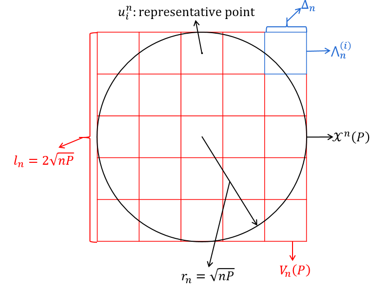
Figure 2: Intuition behind the quantization method.

For a distribution $Q$ supported on $\mathcal{X}^{n}(P)$, we denote $\bar{Q}$ supported on $\mathcal{R}^{n}(P)$ by

$$\bar{Q}(u^{n}_{i})=Q(\Lambda^{(i)}_{n})(i=1,2,...,k_{n}(P)).$$ (7)

When the edge length $\Delta_{n}$ is small enough, the output distribution induced by $\bar{Q}$ approximates the real output distribution induced by $Q$ (see (3)) well. Therefore, the problem boils down to the finite input alphabet $\mathcal{R}_{n}(P)$, which can be solved as that in DMCs.

III Second-Order RID capacity of the AWGNC

In this section, we obtain the second-order RID capacity of the AWGNC (Theorem 1). In the achievability part, we choose the uniform distribution on the power shell as the input distribution $P_{X^{n}}(x^{n})$, so the components of the output distribution $P_{Y^{n}}(y^{n})$ induced by $P_{X^{n}}(x^{n})$ are not i.i.d., thus is complex to analysis. In order to overcome this difficulty, we extend Hayashi’s Theorem [20] by utilizing capacity-achieving output distribution $Q_{Y^{n}}^{*}(y^{n})=\mathscr{N}(0,(1+P)\mathrm{I_{n}})$ as the auxiliary output distribution instead of $P_{Y^{n}}$. In the converse part, the key idea is to quantize the input alphabet and then convert the problem to a DMC scenario, which is solved by Watanabe [22]. This procedure plays an important role in the derivation of the first-order RID capacity of the AWGNC. In order to get the second-order RID capacity, we directly partition the power shell into small sectors. Compared to the partitions on hypercubes in [21], our quantization method is more accurate.

Let $\mathrm{Q^{-1}}(\cdot)$ be the inverse of the complementary CDF of the standard normal distribution. In [22], the second-order RID capacity of the DMCs is proved to have the same form as the transmission capacity. It was shown by Polyanskiy et.al. [32] that the second-order transmission capacity of the AWGNC is

$$\log\mathrm{M}^{*}_{\mathrm{T}}(\epsilon|W^{n})=n\mathrm{C}(P)-\sqrt{n\mathrm{V}(P)}\mathrm{Q}^{-1}(\epsilon)+\mathrm{O}(\log n),$$

where $\mathrm{M}^{*}_{\mathrm{T}}(\epsilon|W^{n})$ is the optimal code size of the transmission code with the maximal block error rate less than $\epsilon$ and $\mathrm{V}(P)=\log^{2}e\frac{P(P+2)}{2(P+1)^{2}}$ is the channel dispersion.

We would naturally ask: whether the second-order RID capacity and transmission capacity still have the same form in AWGNC ? Our answer is “yes”.

   Theorem 1.

Given an AWGNC $W^{n}$, when the type-II error $\mathrm{\delta}$ vanishes, $\forall\ 0<\varepsilon<1$, the optimal code size of RID (defined in $(\ref{eq4})$) is

$$\log\log N^{*}(\varepsilon,\delta|W^{n})= n\mathrm{C}(P)-\sqrt{n\mathrm{V}(P)}\mathrm{Q^{-1}(\varepsilon)}$$

$$+\mathrm{O}(\log n),\qquad\delta\rightarrow 0.$$ (8)

Compared with the first-order approximation (5) given by Han [21], we provide a more accurate approximation which gives the exact second-order term in the asymptotic expansion. We divide the proof into two parts: the achievability part and the converse part.

Proof of achievability. The key point is the extension of Hayashi’s Theorem 1 [20] by utilizing the auxiliary output distribution. The achievability part is a result of Lemma 1.

   Lemma 1.

Given an arbitrary channel $W^{n}$ and input distribution $P_{X^{n}}$, denote by $P_{Y^{n}}$ the output distribution induced by $P_{X^{n}}$. Assume that real numbers $c,c^{\prime},d,d^{\prime},\tau,\zeta>0$ satisfy

$$\zeta\log(\frac{1}{\tau} -1)>\log 2+1,0<\tau<\frac{1}{3},0<\zeta<1,$$

$$1>\frac{1}{c}+\frac{1}{c^{\prime}},f:=1-\frac{1}{d}-\frac{1}{d^{\prime}}>0.$$

Then, for any integer $M>0$ and real number $K>0$, there exists an $(N,\varepsilon,\delta)$-$\mathrm{ID}$ code such that

$$\varepsilon \leq cd\mathrm{Pr}(\tilde{i}(X;Y)\leq\log K),$$ (9)

$$\delta\leq\zeta+c^{\prime}d^{\prime}\frac{1}{K}\lceil\frac{M}{f}\rceil,$$ (10)

$$N=\lfloor\frac{e^{\tau M}}{Me}\rfloor$$ (11)

provided that

$$cd\mathrm{Pr}(\tilde{i}(X;Y)\leq\log K)+c^{\prime}d^{\prime}\frac{1}{K}\lceil\frac{M}{f}\rceil<1,$$ (12)

where $\tilde{i}(X;Y)\triangleq\log\frac{W(Y|X)}{Q_{Y}(Y)}$ and $Q_{Y}(Y)$ is an auxiliary distribution.

In the following, we choose appropriate parameters in Lemma 1 to prove the achievability part.

Let $W^{n}$ be the length-$n$ AWGNC. Choose $Q_{Y^{n}}^{*}$ as the auxiliary output distribution, namely,

$$Q_{Y^{n}}^{*}(y^{n})=\mathscr{N}(0,(1+P)\mathrm{I_{n}}).$$ (13)

Applying the Central Limit Theorem [33], we have

$$\frac{\tilde{i}(x^{n};Y^{n})-n\mathrm{C}(P)}{\sqrt{n\mathrm{V}(P)}} =\frac{\log e}{2\sqrt{n\mathrm{V}(P)}}[\frac{||Y^{n}||^{2}}{1+P}-||Z^{n}||^{2}]$$

$$\Rightarrow\mathscr{N}(0,1),$$ (14)

where $\tilde{i}(x^{n};Y^{n})=\log\frac{W^{n}(Y^{n}|x^{n})}{Q_{Y^{n}}^{*}(Y^{n})}$ and “$\Rightarrow$” means weak convergence.

Set $c=d=1+\frac{2}{n},c^{\prime}=d^{\prime}=n+2,\tau=\frac{1}{n+2},\zeta=\frac{1+\log 2}{\log n}$. For $K>0$, we apply Lemma 1 by setting $M=\lceil\frac{K}{(n+2)^{4}}\rceil$, then, there exist a constant $F>0$ and a sequence of $(N^{*}(\varepsilon,\delta|W^{n}),\varepsilon_{n},\delta_{n})$-ID codes such that

$$\log\log N^{*}(\varepsilon,\delta|W^{n})\geq\log K-F\log n,$$

$$\varepsilon_{n}\leq(1+\frac{2}{n})^{2}\mathrm{Pr}(\tilde{i}(x^{n};Y^{n})\leq\log K),$$

$$\delta_{n}\leq\frac{1+\log 2}{\log n}+\frac{2}{n+2},$$

if

$$(1+\frac{2}{n})^{2}\mathrm{Pr}(\tilde{i}(x^{n};Y^{n})\leq\log K)+\frac{2}{n+2}\leq 1.$$

   Lemma 2.

(Berry-Esseen Theorem for Functions of i.i.d. Random Vectors [33, 34]). Assume that $X_{1}^{k},\ldots,X_{n}^{k}$ are $\mathbb{R}^{k}$-valued, zero-mean, i.i.d. random vectors with positive definite covariance $\operatorname{Cov}\left(X_{1}^{k}\right)$ and finite third absolute moment $\xi:=\mathrm{E}\left[\left\|X_{1}^{k}\right\|_{2}^{3}\right]$. Let $\mathbf{f}(\mathbf{x})$ be a vector-valued function from $\mathbb{R}^{k}$ to $\mathbb{R}^{l}$ that is also twice continuously differentiable in a neighborhood of $\mathbf{x}=\mathbf{0}$. Let $\mathbf{J}\in\mathbb{R}^{l\times k}$ be the Jacobian matrix of $\mathbf{f}(\mathbf{x})$ evaluated at $\mathbf{x}=\mathbf{0}$, i.e., its elements are

$$J_{ij}=\left.\frac{\partial f_{i}(\mathbf{x})}{\partial x_{j}}\right|_{\mathbf{x}=\mathbf{0}},$$

where $i=1,\ldots,l$ and $j=1,\ldots,k$. Then, for every $n\in\mathbb{N}$, we have

$$\sup_{\mathscr{C}\in\mathfrak{C}_{l}}\left|\operatorname{Pr}\left(\mathrm{f}\left(\frac{1}{n}\sum_{i=1}^{n}X_{i}^{k}\right)\in\mathscr{C}\right)-\operatorname{Pr}\left(Z^{l}\in\mathscr{C}\right)\right|\leq\frac{c}{\sqrt{n}}$$

where $c>0$ is a finite constant, and $Z^{l}$ is a Gaussian random vector in $\mathbb{R}^{l}$ with mean vector and covariance matrix respectively given as

$$\mathrm{E}\left[Z^{l}\right]=\mathbf{f}(\mathbf{0}),\quad\text{ and }\quad\operatorname{Cov}\left(Z^{l}\right)=\frac{\mathbf{J}\operatorname{Cov}\left(X_{1}^{k}\right)\mathbf{J}^{\prime}}{n}.$$

Denote for arbitrary $\kappa$

$$\log K=n\mathrm{C}(P)-\kappa\sqrt{n\mathrm{V}(P)}.$$

It is easily to check that for every $x^{n}\in\mathbb{R}^{n}$ such that $\|x^{n}\|_{2}^{2}=nP$, the moments of $\tilde{i}(x^{n};Y^{n})$ satisfy that

$$\mathbb{E}\left[\frac{1}{n}\sum_{i=1}^{n}\log\frac{W\left(Y_{i}\mid x_{i}\right)}{Q_{Y}^{*}\left(Y_{i}\right)}\right] =\mathrm{C}(P),$$

$$\operatorname{Var}\left[\frac{1}{n}\sum_{i=1}^{n}\log\frac{W\left(Y_{i}\mid x_{i}\right)}{Q_{Y}^{*}\left(Y_{i}\right)}\right] =\frac{\mathrm{V}(P)}{n},$$

$$\mathbb{E}\big{|}\frac{1}{n}\sum_{i=1}^{n}\log\frac{W\left(Y_{i}\mid x_{i}\right)}{Q_{Y}^{*}\left(Y_{i}\right)}\big{|}^{3} <+\infty.$$

According to Lemma 2, we have

$$\Big{|}\mathrm{Pr}(\tilde{i}(x^{n};Y^{n})\leq\log K)-\mathrm{Q}(\kappa)\Big{|}\leq\frac{B}{\sqrt{n}},$$ (15)

where $B>0$ is a finite constant.

For sufficiently large $n$, let

$$\kappa=\mathrm{Q}^{-1}((1+\frac{2}{n})^{-2}\varepsilon-\frac{B}{\sqrt{n}}).$$

Then, from (15) we obtain

$$\varepsilon_{n}\leq(1+\frac{2}{n})^{2}\mathrm{Pr}(\tilde{i}(x^{n};Y^{n})\leq\log K)\leq\varepsilon.$$ (16)

Hence,

$$\log\log N^{*}(\varepsilon,\delta|W^{n})\geq n\mathrm{C}(P)-\sqrt{n\mathrm{V}(P)}\mathrm{Q}^{-1}(\varepsilon)$$

$$+\mathrm{O}(\log n),\quad\delta\rightarrow 0.$$ (17)

Proof of converse. In this part, we develop a finer quantization method depicted in Fig 3.

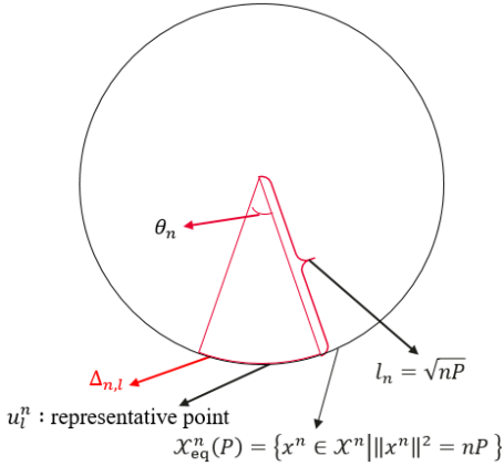
Figure 3: A finer quantization method.

Let us provide some intuition for the quantization method above. First, we partition the power shell $\mathcal{X}_{\mathrm{eq}}^{n}(P)$ into small sectors $\Delta_{n,l}(l=1,\cdots,m_{n}(P))$ with angle $\theta_{n}$. Then, let

$$\mathcal{V}_{n}(P)=\{u^{n}_{1},\cdots,u^{n}_{m_{n}(P)}\}$$

and denote $\bar{Q}$ supported on $\mathcal{V}_{n}(P)$ by

$$\bar{Q}(u^{n}_{l})=Q(\Delta_{n,l})(l=1,2,...,m_{n}(P)),$$ (c)

in other words, $\bar{Q}$ is obtained by concentrating the mass of $Q$ in $\Delta_{n,l}$ to the representative point $u^{n}_{l}$.

When the angel $\theta_{n}$ is small, the output distribution induced by $\bar{Q}$ approximates the real output induced by $Q$ (see (3) by replacing $\mathcal{X}^{n}(P)$ by $\mathcal{X}^{n}_{\mathrm{eq}}(P)$) well. Fig 3 proposes a finer quantization which leads to the second-order RID capacity.

   Remark 1.

Define an $n$-dimensional spherical coordinate system determined by angles $\phi_{1},\cdots,\phi_{n-1}$ and radius $l_{n}$,

$$\begin{cases}x_{1}=l_{n}\cos\phi_{1}\\ x_{2}=l_{n}\sin\phi_{1}\cos\phi_{2}\\ \cdots\\ x_{n-2}=l_{n}\sin\phi_{1}\cdots\sin\phi_{n-2}\cos\phi_{n-1}\\ x_{n-1}=l_{n}\sin\phi_{1}\cdots\sin\phi_{n-2}\sin\phi_{n-1}\end{cases}$$

where $0\leq\phi_{m}\leq\pi(1\leq m\leq n-2)$, $0\leq\phi_{n-1}\leq 2\pi$.

Then, the number of the sectors is

$$m_{n}(P)=(\frac{\pi}{\theta_{n}})^{n-2}\frac{2\pi}{\theta_{n}}.$$ (18)

$\mathbf{Step}$ $\mathbf{1.}$ Let $l_{n}=\sqrt{nP}$ be the radius of the power shell $\mathcal{X}_{\mathrm{eq}}^{n}(P)$ and substitute $\theta_{n}=\exp(-n)$ into $(\ref{eq18})$, we have

$$\frac{\log\log m_{n}(P)}{\log n}\rightarrow C,$$ (19)

where $C>0$ is a constant.

Here, we give a brief proof of (19).

Substituing $\theta_{n}$ into $(\ref{eq18})$, so that $m_{n}(P)$ can be calculated as

$$m_{n}(P)=\frac{2\pi^{n-1}}{(\exp(-n))^{n-1}}.$$ (20)

The result shown in $(\ref{eq19})$ immediately follows by $(\ref{eq111})$.

$\mathbf{Step}$ $\mathbf{2.}$ Using the quantization distribution $\bar{Q}(\cdot)$ given by $\mathrm{(c)}$ and the Pinsker’s inequality, we can show that

$$d(QW^{n},\bar{Q}W^{n})\leq\sqrt{P}n^{3/2}e^{-n}.$$ (21)

Now, we give the proof of $(\ref{eq20})$.

For any $x^{n},u^{n}_{l}\in\Delta_{n,l}$, from the definition of the KL divergence between two multivariate Gaussian distributions, we obtain

$$D(W^{n}(\cdot|x^{n})||W^{n}(\cdot|u^{n}_{l}))=\frac{1}{2}n||x^{n}-u^{n}_{l}||^{2}$$

$$\leq\frac{n(n-1)}{2}(\sqrt{nP}e^{-n})^{2}.$$ (22)

By the Pinsker’s inequality [35] and the triangle inequality, we have

$$d(QW^{n},\bar{Q}W^{n})=2\sup_{\mathcal{B}\subset\mathbb{R}^{n}}|QW^{n}(\mathcal{B})-\bar{Q}W^{n}(\mathcal{B})|$$

$$\leq 2\sum_{l=1}^{m_{n}(P)}\sum_{x^{n}\in\Delta_{n,l}}|W^{n}(\mathcal{B}|x^{n})-W^{n}(\mathcal{B}|u^{n}_{l})|Q(x^{n})$$

$$\leq 2\sum_{l=1}^{m_{n}(P)}\frac{1}{2}\sqrt{2D(W^{n}(\cdot|x^{n})||W^{n}(\cdot|u^{n}_{l}))}\bar{Q}(u^{n}_{l})$$

$$\leq\sqrt{P}n^{3/2}e^{-n}.$$ (23)

$\mathbf{Step}$ $\mathbf{3.}$ Next, we investigate the relation between ID and resolvability [14, 18, 19, 20, 21, 22]. We have the following lemma.

   Lemma 3.

For arbitrary $0<\varepsilon,\ \delta,\ \xi<1$ with $0<\varepsilon+\delta+\xi+\sqrt{P}n^{3/2}e^{-n}<1$, we have

$$\log\log N^{*}(\varepsilon,\delta|W^{n})\leq\log M^{*}(\xi|W^{n})+\mathrm{O}(\log n),$$ (24)

where $N^{*}(\varepsilon,\delta|W^{n})$ and $M^{*}(\xi|W^{n})$ are the optimal code size of the $(\varepsilon,\delta)$-$\mathrm{ID}$ code and the $\xi$-resolvability code, respectively.

Proof.

Let $N_{n}=N^{*}(\varepsilon,\delta|W^{n}),M_{n}=M^{*}(\xi|W^{n})$, by definition, there exist an $(n,N_{n},\varepsilon_{n},\delta_{n})$-ID code and $M_{n}$-type probability distributions $\tilde{Q}_{j}(j=1,\cdots,N_{n})$ supported on $\mathcal{X}_{\mathrm{eq}}^{n}(P)$ satisfying

$$\varepsilon_{n}\leq\varepsilon,\quad\delta_{n}\leq\delta,$$ (25)

$$d(Q_{j}W^{n},\tilde{Q}_{j}W^{n})\leq\xi,$$ (26)

for all $j=1,\cdots,N_{n}$, where $Q_{j}$ is the random encoder.

Let $\bar{\tilde{Q}}_{j}(j=1,\cdots,N_{n})$ be the quantization distribution of the $M_{n}$-type distribution $\tilde{Q}_{j}$. Therefore, $\bar{\tilde{Q}}_{j}$s are also $M_{n}$-types. By (21), we have

$$d(\tilde{Q}_{j}W^{n},\bar{\tilde{Q}}_{j}W^{n})\leq\sqrt{P}n^{3/2}e^{-n}.$$ (27)

Combine (26) and (27), we obtain

$$d(Q_{j}W^{n},\bar{\tilde{Q}}_{j}W^{n})\leq\xi+\sqrt{P}n^{3/2}e^{-n}.$$ (28)

Suppose that there exists $j\neq k$, such that $\bar{\tilde{Q}}_{j}=\bar{\tilde{Q}}_{k}$, then, by the triangular inequality and the definition of the TV distance,

$$2(1-\varepsilon-\delta)\leq d(Q_{j}W^{n},Q_{k}W^{n})\leq 2\xi+2\sqrt{P}n^{3/2}e^{-n},$$

i.e., $\varepsilon+\delta+\xi+\sqrt{P}n^{3/2}e^{-n}\geq 1$, which is a contradiction!

Therefore, $\bar{\tilde{Q}}_{j}(j=1,\cdots,N_{n})$ must be distinct $M_{n}$-type distributions, since the number of distinct $M_{n}$-types is upper bounded by $m_{n}(P)^{M_{n}}$. Hence, it must hold that $N_{n}\leq m_{n}(P)^{M_{n}}$, which implies

$$\log\log N_{n}\leq\log M_{n}+\log\log m_{n}(P).$$ (29)

By (19)

$$\log\log N_{n}\leq\log M_{n}+\mathrm{O}(\log n).$$ (30)

This completes the proof of (24). ∎

A channel $W=\{(\mathcal{X},\mathcal{F}),(\mathcal{Y},\mathcal{G}),K\}$ is defined by an input alphabet $\mathcal{X}$ with $\sigma$-algebra $\mathcal{F}$, an output alphabet $\mathcal{Y}$ with $\sigma$-algebra $\mathcal{G}$, and a stochastic kernel $K$ that specifies the stochastic transition between the input and output alphabets. Subsequently, the lemma presented below provides a second-order achievability bound for the channel resolvability capacity, paving the way for establishing the second-order RID capacity for AWGNCs.

   Lemma 4.

(Frey’s Theorem 3 [36]) Given a channel $W=\{(\mathcal{X},\mathcal{F}),(\mathcal{Y},\mathcal{G}),K\}$ and an input distribution $Q_{X}$ such that the information density $i(X;Y)$ has finite central second moment $V$ and finite absolute third moment $\rho$, $\xi>0$ and $c>1$, suppose the rate $R$ depends on $n$ in the following way:

$$R=I(X;Y)+\sqrt{\frac{V}{n}}\mathrm{Q}^{-1}(\xi)+c\frac{\log n}{n}.$$

Then, for any $d\in(0,c-1)$ and $n$ that satisfy $n^{(c-d)/2}\geq 6$, we have

$$P_{\mathcal{C}} (||P_{Y^{n}[c^{M}]}-QW^{n}||_{2}\geq\mu(1+\frac{1}{\sqrt{n}})+\frac{1}{\sqrt{n}})$$

$$\leq\exp(-\frac{1}{3}n\mu\exp(nR))$$

$$+(\frac{7}{6}+\sqrt{3\pi/2}\exp(\frac{3}{4}))\exp(-n^{\frac{1}{2}(c-d-1)}),$$

where

$$\mu:=\mathrm{Q}(\mathrm{Q}^{-1}(\xi)+d\frac{\log n}{\sqrt{nV}})+\frac{\rho}{V^{\frac{3}{2}}\sqrt{n}}$$

tends to $\xi$ for $n\rightarrow\infty$ and $||x||_{2}$ denote the $\ell^{2}$-norm of $x$.

   Remark 2.

Given that the aforementioned lemma applies to any channel, when we consider the channel as an AWGNC, we can derive the converse bound for the second-order RID capacity of the AWGNCs.

$\mathbf{Step}$ $\mathbf{4.}$ Let

$$\xi=1-\varepsilon-\delta-\sqrt{P}n^{3/2}e^{-n}.$$ (31)

Let $\delta\rightarrow 0$, i.e., the type-II error vanishes, from (24) and Lemma 4, we obtain

$$\log\log N^{*}(\varepsilon,\delta|W^{n})\leq\log M^{*}(\xi|W^{n})+\mathrm{O}(\log n)$$

$$\leq n\mathrm{C}(P)+\sqrt{n\mathrm{V}(P)}\mathrm{Q^{-1}}(1-\varepsilon-\sqrt{P}n^{3/2}e^{-n})+\mathrm{O}(\log n)$$

$$=n\mathrm{C}(P)-\sqrt{n\mathrm{V}(P)}\mathrm{Q}^{-1}(\varepsilon+\sqrt{P}n^{3/2}e^{-n})+\mathrm{O}(\log n)$$

$$\leq n\mathrm{C}(P)-\sqrt{n\mathrm{V}(P)}\mathrm{Q}^{-1}(\varepsilon)+\mathrm{O}(\log n),$$ (32)

where the last inequality is due to the Taylor expansion

$$\mathrm{Q}^{-1}(\varepsilon+\sqrt{P}n^{3/2}e^{-n})$$

$$=\mathrm{Q}^{-1}(\varepsilon)-\underbrace{\left.\frac{d\mathrm{Q}^{-1}(x)}{dx}\right|_{x=\varepsilon}}_{\mathrm{O}(1)}\sqrt{P}n^{3/2}e^{-n}+\mathrm{o}(n^{3/2}e^{-n})$$

$$\geq\mathrm{Q}^{-1}(\varepsilon)+\mathrm{o}(\frac{1}{\sqrt{n}}).$$

Thus, we prove the converse part.

The desired results follow from (17) and (32).∎

IV Conclusion

The second-order RID capacity of the AWGNC has been investigated in this paper. It has been proved that the second-order RID capacity have the same form as the transmission capacity in AWGNC. An extension of Hayashi’s Theorem to the auxiliary output distribution leads to the achievability part and a finer quantization method has been proposed in the proof of the converse part which gives the $\mathrm{O}(\log n)$ term. As a future direction, it is tempting to apply the quantization approach to other identification problems. Furthermore, it remains an open problem to determine the second-order $(\varepsilon,\delta)$-ID capacity of the AWGNC for non-vanishing type-II error $\delta$, i.e., $\delta\geq\varepsilon_{0}$ with $\varepsilon_{0}>0$ a positive constant. It is also an interesting work to derive the third-order $(\varepsilon,\delta)$-ID capacity of the AWGNC.

References

- [1] L. Chettri and R. Bera, “A comprehensive survey on Internet of Things (IoT) toward 5G wireless systems,” IEEE Internet Things J., vol. 7, no. 1, pp. 16–32, Jan. 2020.
- [2] Q. Qi, X. Chen, C. Zhong, and Z. Zhang, “Integration of energy, computation and communication in 6G cellular internet of things,” IEEE Commun. Lett., vol. 24, no. 6, pp. 1333-1337, Jun. 2020.
- [3] H. Boche and C. Deppe, “Secure identification for wiretap channels; robustness, super-additivity and continuity,” IEEE Trans. Inf. Forensics Security, vol. 13, no. 7, pp. 1641–1655, Jul. 2018.
- [4] K. Guan, B. Ai, M. Liso Nicols, R. Geise, A. Mller, Z. Zhong, and T. Krner, “On the influence of scattering from traffic signs in vehicle-to-x communications,” IEEE Trans. Veh. Technol., vol. 65, no. 8, pp. 5835–5849, Aug. 2016.
- [5] J. Choi, V. Va, N. Gonzalez-Prelcic, R. Daniels, C. R. Bhat, and R. W. Heath, “Millimeter-wave vehicular communication to support massive automotive sensing,” IEEE Commun. Mag., vol. 54, no. 12, pp. 160–167, Dec. 2016.
- [6] G. P. Fettweis, “The tactile Internet: Applications and challenges,” IEEE Veh. Technol. Mag., vol. 9, no. 1, pp. 64–70, Mar. 2014.
- [7] N. Michailow, L. Mendes, M. Matthé, I. Gaspar, A. Festag, and G. Fettweis, “Robust WHT-GFDM for the next generation of wireless networks,” IEEE Commun. Lett., vol. 19, no. 1, pp. 106–109, Jan. 2015.
- [8] A. Matveev and A. Savkin, Estimation and Control over Communication Networks. Springer, 2009.
- [9] H. Boche and C. Arendt, “Communication method, mobile unit, interface unit, and communication system,” 2021, patent number: 10959088.
- [10] P. Moulin, “The role of information theory in watermarking and its application to image watermarking,” Signal Processing, vol. 81, no. 6, pp. 1121–1139, 2001.
- [11] Y. Steinberg, “Watermarking identification for private and public users: the broadcast channel approach,” IEEE Inf. Theory Workshop(ITW), 2002, pp. 5–7.
- [12] P. Moulin and R. Koetter, “A framework for the design of good watermark identification codes,” in Security, Steganography, and Watermarking of Multimedia Contents VIII, E. J. D. III and P. W. Wong, Eds., vol. 6072, International Society for Optics and Photonics. SPIE, 2006, pp. 565 – 574.
- [13] S. Derebeyǒglu, C. Deppe, and R. Ferrara, “Performance analysis of identification codes,” Entropy, vol. 22, no. 10, p. 1067, Sep. 2020.
- [14] R. Ahlswede and G. Dueck, “Identification via channels,” IEEE Trans. Inf. Theory, vol. 35, no. 1, pp. 15-29, Jan. 1989.
- [15] C. E. Shannon, “A mathematical theory of communication,” Bell Syst. Tech. J., vol. 27, no. 3, pp. 379-423, Jul. 1948.
- [16] M. V. Burnashev, “On identification capacity of infinite alphabets or continuous-time channels,” IEEE Trans. Inf. Theory, vol. 46, no. 7, pp. 2407–2414, Nov. 2000.
- [17] R. Ferrara, L. Torres-Figueroa, H. Boche, C. Deppe, W. Labidi, U. Mönich, and A. Vlad-Costin, “Implementation and experimental evaluation of Reed–Solomon identification,” in Proc. Eur. Wireless, Sept. 2022, pp. 1–6.
- [18] T. S. Han and S. Verdú, “Approximation theory of output statistics,” IEEE Trans. Inf. Theory, vol. 39, no. 3, pp. 752-772, May 1993.
- [19] Y. Steinberg, “New converses in the theory of identification via channels”, IEEE Trans. Inf. Theory, vol. 44, no. 3, pp. 984-998, 1998.
- [20] M. Hayashi, “General nonasymptotic and asymptotic formulas in channel resolvability and identification capacity and their application to the wiretap channel,” IEEE Trans. Inf. Theory, vol. 52, no. 4, pp. 1562-1575, Apr. 2006.
- [21] T. S. Han, Information-Spectrum Methods in Information Theory, Springer Berlin Heidelberg, 2003.
- [22] S. Watanabe, “Minimax converse for identification via channels,” IEEE Trans. Inf. Theory, vol. 68, no. 1, pp. 25-34, Jan. 2022.
- [23] S. Verdu and V. K. Wei, “Explicit construction of optimal constant-weight codes for identification via channels,” IEEE Trans. Inf. Theory, vol. 39, no. 1, pp. 30–36, Jan. 1993.
- [24] R. Ahlswede and Ning Cai, “Identification without randomization,” IEEE Trans. Inf. Theory, vol. 45, no. 7, pp. 2636–2642, 1999.
- [25] J. JJ, “Identification is easier than decoding,” in Ann. Symp. Found. Comp. Scien. (SFCS), 1985, pp. 43–50.
- [26] M. J. Salariseddigh, U. Pereg, H. Boche, and C. Deppe, “Deterministic identification over fading channels,” in Proc. IEEE Inf. Theory Workshop (ITW), Apr. 2021, pp. 1–5.
- [27] M. J. Salariseddigh, U. Pereg, H. Boche, and C. Deppe, “Deterministic identification over channels with power constraints,” IEEE Trans. Inf. Theory, vol. 68, no. 1, pp. 1–24, Jan. 2022.
- [28] Y. Li, X. Wang, H. Zhang, J. Wang, W. Tong, G. Yan, and Z. Ma, “Deterministic identification over channels without CSI,” in Proc. IEEE Inf. Theory Workshop (ITW), Nov. 2022, pp. 332–337
- [29] W. Labidi, C. Deppe, and H. Boche, “Secure identification for Gaussian channels,” in Proc. IEEE Int. Conf. Acoust., Speech Signal Process. (ICASSP), May 2020, pp. 2872–2876.
- [30] J. Cabrera, H. Boche, C. Deppe, R. F. Schaefer, C. Scheunert, and F. H. Fitzek, “6G and the Post-Shannon theory,” in Shaping Future 6G Networks: Needs, Impacts and Technologies. Hoboken, NJ, USA: Wiley, 2021, pp. 271–294.
- [31] R. Ahlswede, Identification and Other Probabilistic Models, A. Ahlswede, I. Althöfer, C. Deppe, and U. Tamm, Eds. Cham, Switzerland: Springer, 2021.
- [32] Y. Polyanskiy, H. V. Poor, and S. Verdú, “Channel coding rate in the finite blocklength regime,” IEEE Trans. Inf. Theory, vol. 56, no. 5, pp. 2307-2359, May 2010.
- [33] E. MolavianJazi and J. N. Laneman, “A finite-blocklength perspective on Gaussian multi-access channels.” [Online]. Available: http://arxiv.org/abs/1309.2343, 2014.
- [34] V. Y. F. Tan, “Asymptotic estimates in information theory with non-vanishing error probabilities.” Found. Trends Commun. Inf. Theory, vol. 11, no. 1-2, pp. 1-184, 2014.
- [35] M. S. Pinsker, Information and Information Stability of Random Variables and Processes (in Russian). Moscow, U.S.S.R.: Izv. Akad. Nauk, 1960.
- [36] M. Frey, I. Bjelakovic, and S. Stanczak, “Resolvability on continuous alphabets,” in Proc. IEEE Int. Symp. Inf. Theory, Jun. 2018, pp. 2037–2041.