Marangoni Interfacial Instability Induced by Solute Transfer Across Liquid-Liquid Interfaces

Abstract

This study presents analytical and numerical investigations of Marangoni interfacial instability in a two-liquid-layer system with constant solute transfer across the liquid interface. Previous research has demonstrated that both viscosity ratio and diffusivity ratio can influence the system’s hydrodynamic stability via the Marangoni effect, but the distinctions in process and mechanisms are not yet fully understood. To gain insights, we developed a numerical model based on the phase-field method, rigorously validated against linear stability analysis. The parameter space explored encompasses Schmidt number ($Sc\in[0.2,200]$), Marangoni number ($Ma_{c}\in[10,2000]$), Capillary number ($Ca\in[0.01,1]$), viscosity ratio ($\zeta_{\mu}\in[0.1,10]$), and diffusivity ratio ($\zeta_{D}\in[0.1,10]$). We identified two key characteristics of Marangoni instability: the self-amplification of triggered Marangoni flows in flow-intensity-unstable case and the oscillation of flow patterns during flow decay in flow-intensity-stable case. Direct numerical simulations incorporating interfacial deformation and nonlinearity confirm that specific conditions, including solute transfer out of a higher viscous or less diffusive layer, amplify and sustain Marangoni interfacial flows. Furthermore, the study highlights the role of interfacial deformation and unequal solute variation in system instability, proposing corresponding instability mechanisms. Notably, traveling waves are observed in the flow-intensity-stable case, correlating with the morphological evolution of convection rolls. These insights contribute to a comprehensive understanding of Marangoni interfacial instability in multicomponent fluids systems, elucidating the mechanisms underlying variations in viscosity and diffusivity ratios across liquid layers.

1 Introduction

Multicomponent fluids, comprising two or more chemical species, play a ubiquitous role in various natural and industrial processes, spanning from chemical processing (Brennecke & Maginn, 2001), to biofluidic diagnostics (Oertel, 2004) and material manufacturing (Snell & Helliwell, 2005). The inherent variability in their composition arises from spontaneous mass transfer, mixing processes, or chemical reactions, leading to changes in composition-dependent fluid properties such as surface tension, viscosity, and diffusivity. The resulting hydrodynamics phenomena induced by composition variation, including Marangoni flows (Levich & Krylov, 1969; Manikantan & Squires, 2020) and osmosis flows (Velegol et al., 2016; Shim, 2022), can significantly influence the behavior of flow system. As the length scale of the liquid system decreases to the capillary length ($Bo>1$), the interfacial effect begin to dominate over gravitational forces.

Recently, there has been several complex hydrodynamic phenomena reported in multicomponent microfluidic systems, such as spontaneous phase separation (Tan et al., 2016, 2019a; Guo et al., 2021), self-lubrication (Tan et al., 2019b, 2023), self-explosion (Lyu et al., 2021), self-propulsion (Izri et al., 2014; Jin et al., 2017), Marangoni spreading and contracting (Baumgartner et al., 2022; Chao et al., 2022), attraction and chasing (Cira et al., 2015; Li et al., 2023), and targeted-migration of microdroplets (Banerjee et al., 2016; Tan et al., 2021; May et al., 2022), making multicomponent hydrodynamics a subject of great interest to the fluid mechanics community (Maass et al., 2016; Lohse & Zhang, 2020; Manikantan & Squires, 2020; Wang et al., 2022; Shim, 2022; Dwivedi et al., 2022). The phenomena in these small-scaled liquid systems, share the same fact that the coupling of multiple fields is essential to the richness of the emerging interfacial hydrodynamics. Thus, a comprehensive understanding of the interplay at the interface is crucial to the design of micro-flow systems.

In particular, the Marangoni effect, which predates Thomson’s observation of the tears of wine effect in the 19th century, involves a complex interplay among interfacial flow fields, solute concentration fields, and the deformation of the liquid-liquid interfaces. This phenomenon occurs when surface-active solutes, acting as the third component, are unevenly distributed at the interface between immiscible liquids (Levich & Krylov, 1969). These solutes influence the concentration-dependent interfacial surface tension, denoted as $\gamma$, leading to concentration gradients along the interface. This gradient creates an imbalance that triggers non-equilibrium liquid motions, known as solutal Marangoni flow. These emerging flows advectively transport the solutes, fostering interaction between the flow and concentration fields (Manikantan & Squires, 2020). Simultaneously, the directed motion of flow towards the interface induces interfacial deformation, adding another layer of complexity to the coupling process. Consequently, flow field, composition field, the interfacial deformation become intricately intertwined within the solutal Marangoni flow. An essential and fundamental inquiry pertains to the stability of this interfacial coupling.

In a groundbreaking study, Sternling & Scriven (1959) conducted stability analysis and studied Marangoni hydrodynamic instability between two un-equilibriated fluid $without$ interfacial deformation. They summarized that the stability depends on the solute transfer direction, the viscosity and diffusion ratios of fluids on both sides, and the relationship between the surface tension coefficient and the solute concentration. Since then, Marangoni interfacial instability has garnered significant attention, leading to various numerical and experimental investigations aimed at comparing the results obtained by Sternling & Scriven (1959), exploring criteria such as the Marangoni number for instability or oscillatory stability (Wei, 2006; Kovalchuk & Vollhardt, 2006; Schwarzenberger et al., 2014), and examining instability in different flow systems (Degen et al., 1998; Kalliadasis et al., 2003; Kalogirou et al., 2016; Mokbel et al., 2017; Li et al., 2021).

The trigger of the Marangoni flow can be influenced by various factors, including changes in different solute and temperature at the fluid interface. Frenkel & Halpern (2002), Halpern & Frenkel (2003), Wei (2005), and Frenkel & Halpern (2017) investigated the flow-induced Marangoni flow due to the insoluble surfactant by using the linear analysis method. Recently, Kalogirou (2018) discussed how gravity can either stabilize or destabilize the interface, depending on the Bond number. Kalogirou & Blyth (2020) considered surfactants exceeding their critical micelle concentration. Stability in this context is related to the viscosity and thickness ratios of two fluids and the solubility of the surfactant. Temperature differences can also induce Marangoni flow, referred to as thermal Marangoni flow, leading to Bénard-Marangoni instability. Pearson (1958) initiated discussions on the stability of this system, followed by subsequent researchers (Oron et al., 1995; Slavtchev & Mendes, 2004; Nejati et al., 2015). Hu et al. (2021) employed linear stability analysis to assess the effects of the Prandtl and Biot numbers on physical modes, confirming that wave modes are influenced by the Prandtl number and temperature differences between stationary walls.

Besides the different factors that trigger Marangoni instability, researchers have also studied the stability of different physical systems. Some typical physical systems include a free interface (Sternling & Scriven, 1959; Oron et al., 1995; Schwarzenberger et al., 2014; Hu et al., 2021), a Couette-Poiseuille flow in a channel (Kalogirou et al., 2016; Picardo et al., 2016; Kalogirou & Blyth, 2020), an incline interface (Kalliadasis et al., 2003), and even a drop interface (Li et al., 2021; Mao et al., 2023). However, less attention has been paid to the development of different fields, including concentration field, flow field, and interfacial deformation, and particularly in understanding their coupling process during the hydrodynamic instability. The complexity of experimental studies, due to small length and short time scales, presents challenges in elucidating coupling processes and instability mechanisms (Kovalchuk & Vollhardt, 2006; Shin et al., 2016; Li et al., 2021). Direct numerical simulation (DNS) offers a comprehensive exploration of underlying coupling processes. However, most numerical methods for studying Marangoni instability rely on sharp interface models and linear stability analysis, which has limitations in handle large interface deformations and nonlinearities. Although some researchers have extended linear calculations to address nonlinearity  (Wei, 2005; Kalogirou & Blyth, 2020), there remains a gap from real physical systems.

In this work, we propose a numerical model based on phase-field method to investigate Marangoni interfacial flow in a deformable interface, focusing on the coupling processes among multiple fields and gaining insight into the characteristics of Marangoni hydrodynamic instability. Specifically, we analyze the instability of solutal Marangoni flows induced by transverse and sustained solute transfer across an initially flat liquid-liquid interface, neglecting gravitational effects.

The outline of our study begins with the mathematical formulation of the problem in Section 2, where we develop a numerical model (Eqns. 9) by coupling the convective Allen-Cahn equation, advection-diffusion equation, and the Navier-Stokes equations. We then linearize the problem to derive a system of linear equations (Eqns. 14) for linear stability analysis. Section 3 is dedicated to verifying and validating our methods, ensuring the accuracy and reliability of our approach. In Section 4, we conduct a parameter sweep by solving the linear equation system to explore the effects of different parameters on Marangoni interfacial instability, followed by dedicated DNS for specific parameter settings. Moving to Section 5, we investigate how the perturbation-triggered Marangoni interfacial flow self-amplifies by varying viscosity or diffusivity ratio between the two liquid layers, termed as the flow-intensity-unstable case. In Section 6, we shift our focus to studying how the perturbation-triggered Marangoni interfacial flow weaken under varying viscosity or diffusivity ratio, referred to as the flow-intensity-stable case. Here, we pay particular attention to the oscillation of flow patterns during the decay of the flow intensity. Finally, in Section 7, we summarizes the key findings and conclusions drawn from our comprehensive study on Marangoni interfacial instability.

2 Problem Formulation and Methodology

2.1 Mathematical formulation

To simplify the analysis without sacrificing generality, we consider a two-dimensional scenario. As depicted in figure 1($a$), there are two immiscible fluids confined by two infinite flat non-penetrative surface at $y=0$ and $y=4L$, with the interface in the middle at $y=2L$ separating the bottom fluid $\phi_{\text{u}}$ and the top fluid $\phi_{\text{d}}$. The subscripts ‘u’ and ‘d’, representing the upstream phase and downstream phase respectively, denote the direction of mass flux. A downward concentration gradient $\nabla c$ exists perpendicular to the initially flat interface, indicating a upward solute flux from the bottom surface, across the liquid-liquid interface, towards the top surface. The concentration is constant at the surface, i.e. $c(y=0)=G_{c}L$ and $c(y=4L)=0$, where $G_{c}$ represents the characteristic gradient of concentration. Left and right boundary conditions are periodic. To facilitate tracking interfacial deformation, we utilize diffuse interface in the numerical modeling, as depicted in figure 1($b$). Although this transverse mass transfer does not naturally generate the concentration difference along the flat interface, any perturbation of the concentration field can create a non-homogeneous solute distribution at the interface, thereby triggering the solutal Marangoni flows and the circulation pattern of two-dimensional roll cells (Sternling & Scriven, 1959).

The primary focus of this study is the subsequent behavior of the triggered solutal Marangoni flows, specifically under various conditions. For flow-intensity-unstable conditions, the triggered development of flows are amplified and sustained by the continuous mass transfer, whereas flow-intensity-stable conditions result in the dissipation of the flows. To explore this phenomenon, a combination of direct numerical simulation and stability analysis is employed.

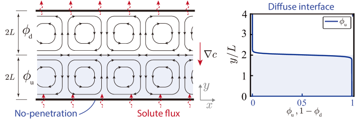
Figure 1: ($a$) Schematic of a two-liquid layer system. There is a constant mass transfer across the interface from the upstream liquid phase $\phi_{\text{u}}$ (blue region) to the downstream one $\phi_{\text{d}}$ (white region). The system is perturbed, triggering Marangoni interfacial flows and the formation of convective rolls formed on both sides. The upper boundary and bottom boundaries are considered non-penertrating and no-slip walls. ($b$) The equilibrium state of the phase parameter distribution $\phi_{\text{u}}$ (blue line) along the $y$-direction, as a diffuse interface is employed. Dirichlet boundary conditions are applied for both solute and phase fields, with periodic boundary conditions at the left and right boundaries.

We use phase field modeling method to numerically simulate the evolution of multicomponent and multiphase interfacial flows. The phase field method is a diffuse interface method of multiphase flow modeling. An order parameter $\phi$ is applied to track the interface and is associated with the free energy functional $\mathcal{E}(\phi)=\int_{\Omega}\left(\frac{1}{2}\epsilon_{1}^{2}|\nabla\phi|^{2}+\epsilon_{2}\phi^{2}(1-\phi)^{2}\right)\text{d}x$. The first term $\epsilon_{1}^{2}|\nabla\phi|^{2}/2$ accounts for the excess free energy of interfacial region, while the second term $\epsilon_{2}\phi^{2}(1-\phi)^{2}$ is a double-well potential function of the bulk energy density to represent the separation of immiscible phases. $\epsilon_{1}$ and $\epsilon_{2}$ are two constants. With the consideration of the advection term, the conservative Allen-Cahn equation introduced by Chiu & Lin (2011) and  Aihara et al. (2019) is applied to capture the deformable interface in a flow field $\boldsymbol{u}$. For the bottom $\phi_{\text{u}}$ and top $\phi_{\text{d}}$ liquid phases, we have two different phase field equations, i.e.,

$$\frac{\partial\phi_{\text{u}}}{\partial t}+\nabla\cdot(\boldsymbol{u}\phi_{\text{u}})=M_{\phi}\left[\nabla\cdot\left(\nabla\phi_{\text{u}}-B\phi_{\text{u}}(1-\phi_{\text{u}})\frac{\nabla\phi_{\text{u}}}{|\nabla\phi_{\text{u}}|}\right)+a_{\text{u}}\right],$$ (1a)

$$\frac{\partial\phi_{\text{d}}}{\partial t}+\nabla\cdot(\boldsymbol{u}\phi_{\text{d}})=M_{\phi}\left[\nabla\cdot\left(\nabla\phi_{\text{d}}-B\phi_{\text{d}}(1-\phi_{\text{d}})\frac{\nabla\phi_{\text{d}}}{|\nabla\phi_{\text{d}}|}\right)+a_{\text{d}}\right],$$ (1b)

where $M_{\phi}$ is a corresponding mobility of phase field to recover the equilibrium profile of interface, and the constant $B=\sqrt{2\epsilon_{2}}/\epsilon_{1}$ is associated with the free energy functional $\mathcal{E}$. To satisfy the constraint condition of $\phi_{\text{u}}+\phi_{\text{d}}=1$, two Lagrange multipliers $a_{1}$ and $a_{2}$ in each phase are employed. The applied form of multipliers is,

$$a_{i}=-\frac{\phi_{i}^{2}}{\phi_{\text{u}}^{2}+\phi_{\text{d}}^{2}}\sum_{j=1}^{2}\left[\nabla\cdot\left(\nabla\phi_{j}-B\phi_{j}(1-\phi_{j})\frac{\nabla\phi_{j}}{|\nabla\phi_{j}|}\right)\right],\quad(i={\text{u}},{\text{d}}),$$ (2)

which is proposed by Lee & Kim (2015) to reduce possible spurious phase formations. The phase field method provides a non-sharp interface, where the equilibrium distribution of variable $\phi$ across the interfacial region is $\phi_{\mathrm{eq}}=\frac{1}{2}\left[1-\tanh\left(B(y-2L)/2\right)\right]$, as depicted by the solid blue line in figure 1b. In the simulation, the constant value $B$ is determined through $B=4/\delta\operatorname{artanh}(1-2\delta_{cr})$. The subscript _cr indicates a truncation of the thickness of an interfacial region $\delta$, and the truncated interfacial region is $\delta_{cr}<\phi_{cr}<1-\delta_{cr}$. In this work, we choose $\delta_{cr}=0.05$ as achievable numerically.

Related to the phase field $\phi$, the fluid properties, including viscosity $\mu$, and solute diffusivity $D$ for the whole computational domain, are assumed by, μ& = μ_u ϕ_u +μ_d ϕ_d,
D = D_u ϕ_u + D_d ϕ_d, We assume the same density value of the two layer fluids, since the gravitational effect is neglected in this work. In the interfacial region, we introduce interfacial surface tension following Kim (2012), reformulated as

$$\boldsymbol{SF}=\frac{1}{2}\left[\gamma\left(\kappa_{\text{u}}\boldsymbol{n}_{\text{u}}+\kappa_{\text{d}}\boldsymbol{n}_{\text{d}}\right)+(\boldsymbol{I}_{\text{u}}-\boldsymbol{n}_{\text{u}}\boldsymbol{n}_{\text{u}}+\boldsymbol{I}_{\text{d}}-\boldsymbol{n}_{\text{d}}\boldsymbol{n}_{\text{d}})\cdot\nabla\gamma\right]W,$$ (3)

where the local normal vector $\boldsymbol{n}_{i}=\nabla\phi_{i}/|\nabla\phi_{i}|$ and curvature $\kappa_{i}=-\nabla\cdot(\nabla\phi_{i}/|\nabla\phi_{i}|)$ are associated with the two phase fields. The $\gamma\kappa\boldsymbol{n}$ term indicates the normal stress due to capillary pressure, and $(\boldsymbol{I}-\boldsymbol{n}\boldsymbol{n})\cdot\nabla\gamma$ is tangential stress because of the Marangoni effect. The weight function $W$ is given by $A\phi_{\text{u}}\phi_{\text{d}}|\nabla\phi_{\text{u}}||\nabla\phi_{\text{d}}|$, and to satisfy the condition of $\int_{-\infty}^{\infty}W\left(\phi_{\text{u}},\phi_{\text{d}}\right)\text{d}y=1$, $A=-30/B$.

By considering an incompressible and isothermal flow with a dilute-solute assumption, we have the governing equations of flow motion expressed as,

$$\rho(\frac{\partial\boldsymbol{u}}{\partial t}+\boldsymbol{u}\cdot\nabla\boldsymbol{u}) =-\nabla p+\nabla\cdot\left[\mu\left(\nabla\boldsymbol{u}+(\nabla\boldsymbol{u})^{T}\right)\right]+\boldsymbol{SF},$$ (4)

$$\nabla\cdot\boldsymbol{u} =0,$$ (5)

and the solute concentration field governed by an advection-diffusion equation

$$\frac{\partial c}{\partial t}+\nabla\cdot(c\boldsymbol{u})=\nabla\cdot(D\nabla c).$$ (6)

As we assume the solute is dilute in this work, the dependence of the fluid properties on the solute concentration is neglected in equation (1). However, a tiny of solute can change the (interfacial) surface tension coefficient $\gamma$ significantly (Khossravi & Connors, 1993; Picardo et al., 2016). Thus, we consider the concentration-surface tension relationship as a linear simplification

$$\gamma=\gamma_{0}-\beta(c-c_{0})\quad(\beta>0),$$ (7)

where $\beta$ is a positive coefficient, and $\gamma_{0}$ indicating the value in the reference state that without solute contaminated.

It is notable that equation (7) associates the flow field $\boldsymbol{u}$ with the concentration field $c$ via the interfacial surface tension term $\boldsymbol{SF}$. Any perturbation of the concentration field can consequently change the flow field, and the flow motion in turn changes the concentration field. So the flow and concentration fields are coupled. Additionally, the flow motion can deform the interface and change the phase field. The deformed interface varies the interfacial surface tension term $\boldsymbol{SF}$, thus the coupling between flow and phase fields also exists. As a result, the two-way coupling between the deformation of fluid-fluid interface, flow field, and concentration field is characterized by the formulated system of equations.

2.2 Non-dimensionlization of governing equations

We adopt the following scalings to non-dimensionalize the governing equation system,

$$\begin{split}&\boldsymbol{x}^{*}=\frac{\boldsymbol{x}}{L},\quad\boldsymbol{u}^{*}=\frac{\boldsymbol{u}}{U},\quad t^{*}=\frac{t}{L/U},\quad p^{*}=\frac{p}{P},\\ &c^{*}=\frac{c}{G_{c}L},\quad\gamma^{*}=\frac{\gamma}{\gamma_{0}},\quad A^{*}=\frac{A}{L},\quad\kappa^{*}=L\kappa,\\ &\mu^{*}=\frac{\mu}{\mu_{\text{u}}}=\phi_{\text{u}}+\frac{1}{\zeta_{\mu}}\phi_{\text{d}},\quad D^{*}=\frac{D}{D_{\text{u}}}=\phi_{\text{u}}+\frac{1}{\zeta_{D}}\phi_{\text{d}}.\end{split}$$ (8)

Here the superscript $*$ designates dimensionless quantities, and $L$, $G_{c}L$, $\gamma_{0}$, $\mu_{\text{u}}$, and $D_{\text{u}}$ are the characteristic scales of length, concentration, interfacial surface tension, density, dynamic viscosity, and solute diffusivity, respectively. $\zeta_{\mu}=\mu_{\text{u}}/\mu_{\text{d}}$ and $\zeta_{D}=D_{\text{u}}/D_{\text{d}}$ are the resulting ratios of dynamic viscosity and diffusivity. To characterize the solutal Marangoni flow in the low Reynold number regime, we use $U=\beta G_{c}L/\mu_{\text{u}}$ as the characteristic velocity, and define the characteristic pressure by $P=\mu_{\text{u}}U/L$. By substituting Eqn. (8) into Eqns. (2.1-2.8), the dimensionless governing equations are obtained as,

$$\frac{\partial\phi_{i}}{\partial t^{*}}+\nabla^{*}\cdot\left(\phi_{i}\boldsymbol{u^{*}}\right)=\frac{1}{Ma_{\phi}}\nabla^{*}\cdot\left[\nabla^{*}\phi_{i}-B^{*}\phi_{i}\left(1-\phi_{i}\right)\frac{\nabla^{*}\phi_{i}}{\left|\nabla^{*}\phi_{i}\right|}\right]+a^{*}_{i},\quad i=\text{u}\,\text{or}\,\text{d},$$ (9a)

$$\frac{\partial c^{*}}{\partial t^{*}}=\frac{1}{Ma_{c}}\nabla^{*}\cdot\left[D^{*}(\nabla^{*}c^{*})\right]-\nabla^{*}\cdot(c^{*}\boldsymbol{u}^{*}),$$ (9b)

$$\frac{\partial\boldsymbol{u^{*}}}{\partial t^{*}}+\boldsymbol{u^{*}}\cdot\nabla^{*}\boldsymbol{u^{*}}=\frac{Sc}{Ma_{c}}\bigg{\{}-\nabla^{*}p^{*}+\nabla^{*}\cdot\left[\mu^{*}\left(\nabla^{*}\boldsymbol{u^{*}}+(\nabla^{*}\boldsymbol{u^{*}})^{T}\right)\right]+\frac{1}{Ca}\boldsymbol{SF}^{*}\bigg{\}},$$ (9c)

$$\nabla^{*}\cdot\boldsymbol{u}^{*}=0,$$ (9d)

$$\boldsymbol{SF^{*}}=\frac{1}{2}\Big{[}\gamma^{*}\left(\kappa^{*}_{\text{u}}\boldsymbol{n}_{\text{u}}+\kappa^{*}_{\text{d}}\boldsymbol{n}_{\text{d}}\right)+(\boldsymbol{I}_{\text{u}}-\boldsymbol{n}_{\text{u}}\boldsymbol{n}_{\text{u}}+\boldsymbol{I}_{\text{d}}-\boldsymbol{n}_{\text{d}}\boldsymbol{n}_{\text{d}})\cdot\nabla^{*}\gamma^{*}\Big{]}W^{*},$$ (9e)

$$\gamma^{*}=1-Ca(c^{*}-c^{*}_{0}).$$ (9f)

The defined dimensional numbers include the Marangoni number of phase field $Ma_{\phi}=UL/M_{\phi}$, the Marangoni number of solute concentration field $Ma_{c}=UL/D_{\text{u}}$, the Schmidt number $Sc=\mu_{\text{u}}/(\rho D_{\text{u}})$, and the Capillary number $Ca=U\mu_{\text{u}}/\gamma_{0}$. We note that $Re=\rho LU/\mu_{\text{u}}=Ma_{c}/Sc$, and $D^{*}$ and $\mu^{*}$ are functions of diffusivity ratio $\zeta_{D}$ and dynamic viscosity ratio $\zeta_{\mu}$, respectively. $Ma_{\phi}$ describes the relative mass transfer of a phase field $\phi$ due to convective deformation and diffusion restoring equilibrium when tracking the interfacial deformation.

2.3 Linear stability analysis

To study the instability onset that induced by the solute concentration gradients on the interface, we perform a linear stability analysis of the flow. We note that the original equation system (9) can be written into a simple form as follows for the convenience of performing linear stability analysis. First, in terms of the phase field variables, due to the constraint $\phi_{\text{u}}+\phi_{\text{d}}=1$, these relations hold

$$\phi_{\text{d}}=1-\phi_{\text{u}},\boldsymbol{n}_{\text{d}}=-\boldsymbol{n}_{\text{u}},\kappa_{\text{d}}=-\kappa_{\text{u}}.$$ (10)

Thus, only one phase field equation needs to be solved. In the present implementation, we choose to solve the equation of $\phi_{\text{u}}$. Second, from expressions in (10), the surface tension term (9e) can be written as

$$\boldsymbol{SF^{*}}=\Big{[}\gamma^{*}\kappa^{*}_{\text{u}}\boldsymbol{n}_{\text{u}}+(\boldsymbol{I}_{\text{u}}-\boldsymbol{n}_{\text{u}}\boldsymbol{n}_{\text{u}})\cdot\nabla^{*}\gamma^{*}\Big{]}W^{*}\,$$ (11)

where $W^{*}=A^{*}\phi_{\text{u}}(1-\phi_{\text{u}})|\nabla^{*}\phi_{\text{u}}|^{2}$. In the framework of linear stability analysis, we decompose the state vector $\boldsymbol{q}^{*}=(\boldsymbol{u}^{*},p^{*},c^{*},\phi_{\text{u}})^{T}$ into a base state $(\boldsymbol{U}^{b},P^{b},C^{b},\phi_{\text{u}}^{b})^{T}$ plus a small perturbation $(\boldsymbol{u}^{\prime},p^{\prime},c^{\prime},\phi_{\text{u}}^{\prime})^{T}$ as

$$\boldsymbol{u}^{*}=\boldsymbol{U}^{b}+\boldsymbol{u}^{\prime},\ \ \ \ p^{*}=P^{b}+p^{\prime},\ \ \ c^{*}=C^{b}+c^{\prime},\ \ \ \phi_{\text{u}}=\phi_{\text{u}}^{b}+\phi^{\prime}_{\text{u}}.$$ (12)

The base state is the solution to the equation system at steady state and it can be derived analytically

$$\boldsymbol{U}^{b}=\boldsymbol{0},\ \ \ \ P^{b}=\text{const.},\ \ \ C^{b}=\frac{c^{*}(4)-c^{*}(0)}{\int_{0}^{4}1/D^{b}\,dy}\int_{0}^{y^{*}}\frac{1}{D^{b}}\,dy^{*}+c^{*}(0),$$

$$\phi_{\text{u}}^{b}=\phi_{\mathrm{eq}}=\frac{1}{2}\left[1-\tanh\left(B^{*}(y^{*}-2)/2\right)\right].$$ (13)

Linearization of the nonlinear equation system (9) is done by substituting the decomposition (12) and then subtracting the corresponding steady base-state equations and finally discarding the nonlinear terms. This process leads to the following linear equation system

$$\frac{\partial\phi^{\prime}_{\text{u}}}{\partial t^{*}}=-\frac{d\phi_{\text{u}}^{b}}{dy^{*}}v^{\prime}+\frac{1}{Ma_{\phi}}\nabla^{*2}\phi^{\prime}_{\text{u}}-\frac{1}{Ma_{\phi}}\frac{\partial^{2}\phi^{\prime}_{\text{u}}}{\partial x^{*2}}-\frac{1}{Ma_{\phi}}B^{*}\left[(2\phi_{\text{u}}^{b}-1)\frac{\partial\phi^{\prime}_{\text{u}}}{\partial y^{*}}+2\frac{d\phi_{\text{u}}^{b}}{dy^{*}}\phi^{\prime}_{\text{u}}\right],$$ (14a)

$$\frac{\partial c^{\prime}}{\partial t^{*}}= -\frac{dC^{b}}{dy^{*}}v^{\prime}+\frac{1}{Ma_{c}}\left(\frac{dD^{b}}{dy^{*}}\frac{\partial c^{\prime}}{\partial y^{*}}+D^{b}\nabla^{*^{2}}c^{\prime}\right)$$

$$+\frac{1}{Ma_{c}}\left[\left(1-\frac{1}{\zeta_{D}}\right)\frac{dC^{b}}{dy^{*}}\frac{\partial\phi^{\prime}_{\text{u}}}{\partial y^{*}}+\left(1-\frac{1}{\zeta_{D}}\right)\frac{d^{2}C^{b}}{dy^{*2}}\phi^{\prime}_{\text{u}}\right],$$ (14b)

$$\rho^{b}\frac{\partial{u}^{\prime}}{\partial t^{*}}= \frac{Sc}{Ma_{c}}\left(-\frac{\partial p^{\prime}}{\partial x^{*}}+\mu^{b}\nabla^{*2}{u}^{\prime}+\frac{d\mu^{b}}{dy^{*}}\frac{\partial{u}^{\prime}}{\partial y^{*}}+\frac{d\mu^{b}}{dy^{*}}\frac{\partial{v}^{\prime}}{\partial x^{*}}\right)$$

$$+\frac{Sc}{Ma_{c}}\left[\frac{1}{Ca}A^{*}\phi_{\text{u}}^{b}(1-\phi_{\text{u}}^{b})\left|\frac{d\phi_{\text{u}}^{b}}{dy^{*}}\right|\frac{d\Gamma^{b}}{dy^{*}}\frac{\partial\phi^{\prime}_{\text{u}}}{\partial x^{*}}-\frac{\partial c^{\prime}}{\partial x^{*}}W^{b}\right],$$ (14c)

$$\rho^{b}\frac{\partial{v}^{\prime}}{\partial t^{*}}= \frac{Sc}{Ma_{c}}\left(-\frac{\partial p^{\prime}}{\partial y^{*}}+\mu^{b}\nabla^{*2}{v}^{\prime}+2\frac{d\mu^{b}}{dy^{*}}\frac{\partial{v}^{\prime}}{\partial y^{*}}\right)$$

$$+\frac{Sc}{Ma_{c}}\left[\frac{1}{Ca}A^{*}\phi_{\text{u}}^{b}(1-\phi_{\text{u}}^{b})\left|\frac{d\phi_{\text{u}}^{b}}{dy^{*}}\right|{\Gamma^{b}}\frac{\partial^{2}\phi^{\prime}_{\text{u}}}{\partial x^{*2}}\right],$$ (14d)

$$0=\frac{\partial u^{\prime}}{\partial x^{*}}+\frac{\partial v^{\prime}}{\partial y^{*}}.$$ (14e)

Here, $\Gamma^{b}=1-Ca(C^{b}-c_{0}^{*})$, $c_{0}^{*}=0$, and $W^{b}=A^{*}\phi_{\text{u}}^{b}(1-\phi_{\text{u}}^{b})|\nabla^{*}\phi_{\text{u}}^{b}|^{2}$. For the boundary conditions, as the base state solutions $\boldsymbol{U}^{b}$, $C^{b}$ and $\phi_{\text{u}}^{b}$ in (2.3) have already satisfied their Dirichlet boundary conditions, the perturbative variables $\boldsymbol{u}^{\prime}=\boldsymbol{0}$, $c^{\prime}=0$ and $\phi^{\prime}_{\text{u}}=0$ should be enforced at the walls for solving (14).

The linear equation system (14) admits normal mode solutions in the form of

$$\boldsymbol{u}^{\prime}=\tilde{\boldsymbol{u}}(y^{*})\text{e}^{\text{i}kx^{*}-\text{i}\omega t^{*}}+\text{c.c.},\ \ \ p^{\prime}=\tilde{p}(y^{*})\text{e}^{\text{i}kx^{*}-\text{i}\omega t^{*}}+\text{c.c.},$$

$$c^{\prime}=\tilde{c}(y^{*})\text{e}^{\text{i}kx^{*}-\text{i}\omega t^{*}}+\text{c.c.},\ \ \ \phi^{\prime}_{\text{u}}=\tilde{\phi}_{\text{u}}(y^{*})\text{e}^{\text{i}kx^{*}-\text{i}\omega t^{*}}+\text{c.c.}(k\neq 0),$$ (15)

where i is the imaginary unit, $k$ is the real-valued wavenumber, $\omega=\omega_{r}+\text{i}\omega_{i}$ is the complex frequency with $\omega_{i}$ being the linear growth rate and $\omega_{r}$ being the oscillation frequency of energy, variables marked with tilde $\tilde{}$ are related to the eigenfunction calculations, c.c. represents the complex conjugate of its preceding term. To interpret the results from the linear stability analysis, $\omega_{i}>0$ indicates that the triggered Marangoni flow is linearly unstable to infinitesimal disturbances; a negative value means it is linearly stable; being zero corresponds to a neutral state. And $\omega_{r}\neq 0$ signifies that the system’s energy will undergo oscillations throughout its development process. Inserting (2.3) into (14) and equating the terms of the same mode (terms with $\text{e}^{\text{i}kx^{*}-\text{i}\omega t^{*}}$) results in the linear equation system in Fourier space

$$-\text{i}\omega{\tilde{\phi}_{\text{u}}}= -\frac{d\phi_{\text{u}}^{b}}{dy^{*}}\tilde{v}+\frac{1}{Ma_{\phi}}(\frac{d^{2}}{dy^{*2}}-k^{2})\tilde{\phi}_{\text{u}}+$$ (16a)

$$\frac{1}{Ma_{\phi}}k^{2}{\tilde{\phi}_{\text{u}}}-\frac{1}{Ma_{\phi}}B^{*}\left[(2\phi_{\text{u}}^{b}-1)\frac{\partial\tilde{\phi}_{\text{u}}}{\partial y^{*}}+2\frac{d\phi_{\text{u}}^{b}}{dy^{*}}\tilde{\phi}_{\text{u}}\right].$$ (16b)

$$-\text{i}\omega{\tilde{c}}= -\frac{dC^{b}}{dy^{*}}\tilde{v}+\frac{1}{Ma_{c}}\left[\frac{dD^{b}}{dy^{*}}\frac{\partial\tilde{c}}{\partial y^{*}}+D^{b}\left(\frac{d^{2}}{dy^{*2}}-k^{2}\right)\tilde{c}\right]$$

$$+\frac{1}{Ma_{c}}\left[\left(1-\frac{1}{\zeta_{D}}\right)\frac{dC^{b}}{dy^{*}}\frac{\partial\tilde{\phi}_{\text{u}}}{\partial y^{*}}+\left(1-\frac{1}{\zeta_{D}}\right)\frac{d^{2}C^{b}}{dy^{*2}}\tilde{\phi}_{\text{u}}\right],$$ (16c)

$$-\text{i}\omega\rho^{b}\tilde{u}= \frac{Sc}{Ma_{c}}\left[-\text{i}k\tilde{p}+\mu^{b}\left(\frac{d^{2}}{dy^{*2}}-k^{2}\right)\tilde{u}+\frac{d\mu^{b}}{dy^{*}}\frac{\partial\tilde{u}}{\partial y^{*}}+\text{i}k\frac{d\mu^{b}}{dy}{\tilde{v}}\right]$$

$$+\frac{Sc}{Ma_{c}}\left[\frac{1}{Ca}A^{*}\phi_{\text{u}}^{b}(1-\phi_{\text{u}}^{b})\left|\frac{d\phi_{\text{u}}^{b}}{dy^{*}}\right|\frac{d\Gamma^{b}}{dy^{*}}\text{i}k{\tilde{\phi}_{\text{u}}}-\text{i}k{\tilde{c}}W^{b}\right],$$ (16d)

$$-\text{i}\omega\rho^{b}{\tilde{v}}= \frac{Sc}{Ma_{c}}\left[-\frac{\partial\tilde{p}}{\partial y^{*}}+\mu^{b}\left(\frac{d^{2}}{dy^{*2}}-k^{2}\right)\tilde{v}+2\frac{d\mu^{b}}{dy^{*}}\frac{\partial\tilde{v}}{\partial y^{*}}\right]$$

$$+\frac{Sc}{Ma_{c}}\left[\frac{1}{Ca}A^{*}\phi_{\text{u}}^{b}(1-\phi_{\text{u}}^{b})\left|\frac{d\phi_{\text{u}}^{b}}{dy^{*}}\right|{\Gamma^{b}}(-k^{2}){\tilde{\phi}_{\text{u}}}\right],$$ (16e)

$$0=\text{i}k{\tilde{u}}+\frac{\partial\tilde{v}}{\partial y^{*}}.$$ (16f)

By denoting the state vector of the eigenfunctions $\tilde{\boldsymbol{q}}=(\tilde{u},\tilde{v},\tilde{p},\tilde{c},\tilde{\phi}_{\text{u}})^{T}$, the above equation system can be further expressed compactly in a matrix form of

$$\omega\widetilde{\boldsymbol{M}}\tilde{\boldsymbol{q}}=\widetilde{\boldsymbol{L}}\tilde{\boldsymbol{q}},$$ (17)

which is a generalized eigenvalue problem, readily solvable in MATLAB using the functions ‘eig’ (for the whole eigenspectrum) and ‘eigs’ (for the few most unstable eigenmodes). The explicit expressions of the elements in matrices $\widetilde{\boldsymbol{M}}$ and $\widetilde{\boldsymbol{L}}$ can be easily derived by matching with the equation (16).

3 Numerical Method, Verification, and Validation

In this section, we compare the results between DNS of the equation (9) and the linear analysis solution of the equation (16), validating the both methods. We determine the Marangoni flow stability of the system by examining the $\omega_{i}$ and the oscillation characteristic by calculating the $\omega_{r}$.

3.1 Numerical method and data analysis method

We numerically solve the non-dimensionalized governing equations, using a self-developed finite-difference-method solver. For the time derivative terms in the phase field equations and solute equations, a third order Runge-Kutta method is applied. A fifth-order WENO method is used to solve the advection terms in the phase field equation (9a) and the NS equation (9c), following with Aihara et al. (2019). A simple second-order central difference method is applied on the advection term in the solute equation (9b) because the perturbation of solute is random in space and magnitude. For all diffusion terms, we solve them by using the second-order central difference method. The initial condition of solute distribution at difference cases is given by equation (2.3).

For the stability analysis at different modes, we perform a Fast Fourier Transform (FFT) along the interfacial direction ($x$-direction) to transform the DNS results from spatial coordinates $(x^{*},y^{*})$ to spectral space $(k,y^{*})$, yielding the velocity field $\hat{u}(k,\,y^{*},\,t^{*})$ and $\hat{v}(k,\,y^{*},\,t^{*})$, with $k$ presenting the wave number in spectral space. Variables marked with hat $\hat{}$ are related to DNS calculations. Subsequently, we compute the magnitude of the system’s kinetic energy in a spectral space, denoted as $\hat{E}_{\text{ke}}$, at specific time instances and $k$-th mode, by integrating the velocities in $y$-direction,

$$\hat{E}_{\text{ke}}(k,t^{*})=\int_{l_{y}}\left(|\hat{u}(k,y^{*},t^{*})|^{2}+|\hat{v}(k,y^{*},t^{*})|^{2}\right)dy^{*}.$$ (18)

The expression $(k,t^{*})$ represents the dependency of the variable on the $k$-th mode at time $t^{*}$. In DNS, the smallest wave number, $k_{min}$, is dependent on the length of computational domain and is defined as $k_{min}=2\pi/(N_{x}\mathrm{\Delta}x)$, where $N_{x}$ is the number of grids in $x-$direction and $\Delta x$ is the width of grids. The linear growth rate of kinetic energy obtained by DNS for the $k$-th mode is defined as

$${\omega_{i}}(k)=\frac{1}{2}\frac{\ln\left[\hat{E}_{\text{ke}}(k,t^{*}+\mathrm{\Delta}t)/\hat{E}_{\text{ke}}(k,t^{*})\right]}{\mathrm{\Delta}t},$$ (19)

and the $\omega_{r}$ is calculated by

$${\omega_{r}}(k)=\frac{\pi}{\hat{T}(k)},$$ (20)

where $\hat{T}(k)$ is the time period of $k$-th mode. By applying this post-processing technique, we can calculate a series of $\omega_{i}$ and $\omega_{r}$ with different $k$ from the simulation data.

3.2 Numerical method validation

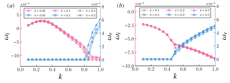
Figure 2: The convergence of $\omega_{i}$ and $\omega_{r}$ under different numerical settings for interface thickness $\delta$. The physical parameters used are set as $Sc=5$, $Ma_{c}=200$, $Ca=1$. In panel ($a$), where $\zeta_{\mu}=10$ and $\zeta_{D}=1$, different curves represent the behavior of $\omega_{i}$ (red lines) and $\omega_{r}$ (blue lines) as the wavenumber $k$ changes. Each curves corresponds to a different value of interface thickness $\delta$. In panel ($b$), the parameters are $\zeta_{\mu}=1$ and $\zeta_{D}=2$, with the same settings as in panel ($a$), showing similar variations in $\omega_{i}$ and $\omega_{r}$ with changes in the wavenumber $k$ and different values of interface thickness $\delta$.

Due to the diffuse interface nature of the phase field method, the interface thickness $\delta$ is a crucial physical parameter to the accuracy of simulation (Demont et al., 2023). Prior to investigating the Marangoni instability, it is necessary to determine an appropriate value for the $\delta$. We employed linear stability analysis to evaluate the impact of interface thickness on $\omega_{i}$ and $\omega_{r}$ for two different cases, as shown in figure 2. Considering the results from both cases, when $\delta\leq 0.1$, the differences are negligible. Taking into account the computational efficiency of DNS, we ultimately chose $\delta=0.1$. According to Jacqmin (1999) and Demont et al. (2023), the $M_{\phi}$ is related to the $\delta$, which is recommended that $M_{\phi}\propto\delta^{a}$ and $a\in(0,3)$. Here, we determine $a\approx 1.7$ and make the $M_{\phi}=0.02$, the $Ma_{\phi}$ is resulted in 50. As the equilibrium state of $\phi$ is determined by the hyperbolic tangent function, typically requiring at least four grid points to describe the interface variation. Therefore, the DNS grid points in the $y$-direction $N_{j}$ should be larger than 160, and it is set to 400 in this study. In the $x$-direction, where the energy of high $k$-th mode usually decays rapidly, and $N_{i}=100$.

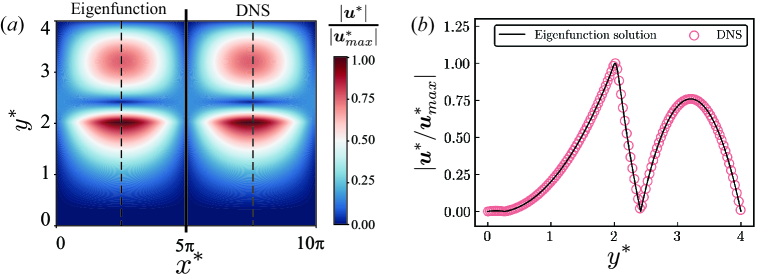
Figure 3: ($a$) Comparison of streamline patterns and velocity contours. The right side displays results obtained through DNS of the equation system (9), while the left side depicted outcomes calculated by solving eigenfunctions (16). The color representation illustrates the normalized velocity magnitude, denoted as $|\boldsymbol{u}^{*}/\boldsymbol{u}^{*}_{max}|$, and $|\boldsymbol{u}^{*}_{max}|$ is the maximum velocity magnitude. ($b$) Comparison of velocity profile $|\boldsymbol{u}^{*}/\boldsymbol{u}^{*}_{max}|$ at $x^{*}=l_{x}/2=5\pi$, emphasizing the agreement between the results obtained from DNS (red dots) and eigenfunctions (dark line).

We conducted a comparative analysis between DNS results and those derived from linear analysis. The validation process commenced with the execution of DNS on the complete governing equations system (9) to acquire the flow fields. Subsequently, we juxtaposed the DNS results with the solution obtained from the eigenfunctions (16). The computational physical region is defined as $l_{y}=4$ and $l_{x}=10\pi$. The physical parameters are set as follows, $Ma_{c}=200$, $Sc=5$, $Ca=1$, $\zeta_{\mu}=10$, $\zeta_{D}=1$. In figure 3($a$), a good agreement is depicted between the streamline patterns and flow intensities, with the eigenfunction solution presented on the left side and the corresponding DNS results on the right side. figure 3($b$) further emphasizes the coherence of the velocity profile at $x^{*}=5\pi$, as determined from DNS (depicted as red circles) and eigenfunctions (illustrated as a dark line). This consistency confirms the precision and reliability of our numerical method in faithfully representing the underlying physical phenomena in the system.

4 Physical Parameter Space and Numerical Investigation

Eigenfunction Settings						Marangoni instability and Oscillation
$Sc$	$Ma_{c}$	$Ca$	$\zeta_{\mu}$	$\zeta_{D}$		Amplified ($\omega_{i}<0$)	Oscillating ($\omega_{r}\neq 0$)
$[0.24,240]$	1200	1	1	1		no amplification	no oscillation
$30$	$[10,2000]$	1	1	1		no amplification	no oscillation
30	1200	$[0.01,1]$	1	1		no amplification	no oscillation
30	1200	1	$[0.1,10]$	1		$\zeta_{\mu}\in[1.32,10]$	$\zeta_{\mu}\in[0.1,1)$
30	1200	1	1	$[0.1,10]$		$\zeta_{D}\in[0.1,0.69]$	$\zeta_{D}\in(1,10]$

Table 1: List of eigenfunction solutions (16) with linear assumption showing the self-amplified Marangoni interfacial flow and oscillatory decay regimes via variations in physical parameters of Schmidt number $Sc$, Marangoni number $Ma_{c}$, Capillary number $Ca$, dynamic viscosity ratio $\zeta_{\mu}$, and diffusivity ratio $\zeta_{D}$.

To investigate the effect of physical parameters on the system stability, we started with a parameter sweep by solving the linear equation system (16). The identified five physical parameters are Schmidt number $Sc=\mu_{\text{u}}/(\rho D_{\text{u}})$, Marangoni number $Ma_{c}=\beta G_{c}L^{2}/(\mu_{\text{u}}D_{\text{u}})$, Capillary number $Ca=U\mu_{\text{u}}/\gamma_{0}$, dynamic viscosity ratio $\zeta_{\mu}=\mu_{\text{u}}/\mu_{\text{d}}$, and diffusivity ratio $\zeta_{D}=D_{\text{u}}/D_{\text{d}}$. The calculated physical parameter space is the specified regime of $Sc\in[0.2,200]$, $Ma_{c}\in[10,2000]$, $Ca\in[0.01,1]$, $\zeta_{\mu}\in[0.1,10]$, and $\zeta_{D}\in[0.1,10]$ as listed in table 1.

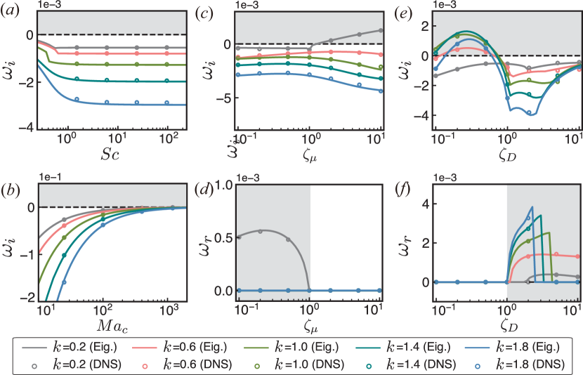
Figure 4: Influence of physical parameters $Sc$ ($a$), $Ma_{c}$ ($b$), $\zeta_{\mu}$ ($c$ and $d$) and $\zeta_{D}$ ($e$ and $f$) on Marangoni interfacial instability. The DNS results (Eqns. 9) are represented by circular dots, while the results from linear stability analysis, obtained by solving the eigenfunction (Eqns. 16), are depicted with solid lines. Different colors correspond to different wave numbers $k=0.2,0.6,1.0,1.4,$ and $1.8$. In the investigated regime of $Sc\in[0.24,240]$ with $Ma_{c}=1200$ ($a$) and $Ma_{c}\in[10,2000]$ with $Sc=30$ ($b$), and when $Ca=1,\zeta_{\mu}=1,\zeta_{D}=1$, the growth rates $\omega_{i}$ for various wave numbers are negative, indicating flow-intensity stability (white region). However, at $Sc=30,Ma_{c}=1200,Ca=1$, when $\zeta_{\mu}>1$ or $\zeta_{D}<1$, the growth rate $\omega_{i}$ becomes positive, indicating flow-intensity-unstable cases (gray region). Conversely, when $\zeta_{\mu}<1$ or $\zeta_{D}>1$, the oscillation frequency $\omega_{r}$ tends towards non-zero values, indicative of oscillatory decay (gray region).

DNS Settings							Marangoni interfacial instability
#	Sc	$Ma_{c}$	$Ca$	$\zeta_{\mu}$	$\zeta_{D}$		Flow-intensity-unstable	Oscillatory decay
1	1.5	1200	1	1	1		$\times$	$\times$
2	6	1200	1	1	1		$\times$	$\times$
3	24	1200	1	1	1		$\times$	$\times$
4	96	1200	1	1	1		$\times$	$\times$
5	30	25	1	1	1		$\times$	$\times$
6	30	100	1	1	1		$\times$	$\times$
7	30	400	1	1	1		$\times$	$\times$
8	30	1600	1	1	1		$\times$	$\times$
9	30	1200	1	0.1	1		$\times$	$\checkmark$
10	30	1200	1	0.2	1		$\times$	$\checkmark$
$11^{c}$	30	1200	1	0.5	1		$\times$	$\checkmark$
12	30	1200	1	1	1		$\times$	$\times$
13	30	1200	1	2	1		$\checkmark$	$\times$
14	30	1200	1	5	1		$\checkmark$	$\times$
$15^{a}$	30	1200	1	10	1		$\checkmark$	$\times$
16	30	1200	1	1	0.1		$\checkmark$	$\times$
$17^{b}$	30	1200	1	1	0.2		$\checkmark$	$\times$
18	30	1200	1	1	0.5		$\checkmark$	$\times$
19	30	1200	1	1	2		$\times$	$\checkmark$
$20^{d}$	30	1200	1	1	5		$\times$	$\checkmark$
21	30	1200	1	1	10		$\times$	$\checkmark$

Table 2: Summary of DNS results (Eqns. 9) with corresponding physical parameters. ‘$\checkmark$’ indicates self-amplification of the triggered Marangoni interfacial flow or oscillatory decay.
^a Strengthening flow intensity with a viscosity ratio (Sec. 5.1 and Fig. 6).
^b Strengthening flow intensity with a diffusivity ratio (Sec. 5.2 and Fig. 7).
^c Decaying flow intensity and oscillation with a viscosity ratio (Sec. 6.1 and Fig. 8).
^d Decaying flow intensity and oscillation with a diffusivity ratio (Sec. 6.2 and Fig. 10).

The determination of the self-amplified Marangoni interfacial flow and the oscillating decay rely on the calculation of the energy growth rate $\omega_{i}$ and the oscillation frequency $\omega_{r}$, respectively. Negative growth rate leads to the decay of the triggered flow, implying a stable Marangoni interfacial flow, and the oscillating flow pattern exhibits when $\omega_{r}\neq 0$. Table 1 summaries the calculated results and the corresponding parameter settings. For the case of two liquid phases with identical dynamic viscosity ($\zeta_{\mu}=1$) and diffusivity ($\zeta_{D}=1$), the Marangoni flow remains stable either by varying the $Sc$ from 0.24 to 240, or by varying $Ca$ from 0.01 to 1, or by varying $Ma_{c}$ from 10 to 2000. However, by individually varying $\zeta_{\mu}$ from 0.1 to 10 and $\zeta_{D}$ from 0.1 to 10 with $Sc=30$ and $Ma_{c}=1200$, we find $\omega_{i}>0$ in the regimes of $\zeta_{\mu}\in[1.32,10]\,\&\,\zeta_{D}=1$ and $\zeta_{D}\in[0.1,0.69]\,\&\,\zeta_{\mu}=1$, where the triggered Marangoni flow rises up continuously, leading to an unstable case. The DNS results obtained by solving equations (9), as represented in figure 4 align with the eigenfunction solutions, where circular dots for the DNS results and the solid lines for the eigenfunction solutions. There are total 21 sets of ($Sc,Ma_{c},Ca,\zeta_{\mu},\zeta_{D}$) selected from the identified parameter space for the DNS investigation, as detailed in Table 2(#9 - #21).

Additionally, within the stable regimes of the Marangoni flow where the flow decays, we find oscillating regimes occur at $\zeta_{\mu}\in[0.1,1)\,\&\,\zeta_{D}=1$ and $\zeta_{D}\in(1,10]\,\&\,\zeta_{\mu}=1$, Although the impact of $\zeta_{\mu}$ and $\zeta_{D}$ on the stability of the system has been previously reported by Sternling & Scriven (1959) and Kovalchuk & Vollhardt (2006), we highlight here that strengthening of Marangoni flow intensity (flow-intensity-unstable case) and oscillating flow fields during the decaying of Marangoni flow intensity (flow-intensity-stable case) are the two distinct characteristics of hydrodynamic instability that triggered by the perturbation. It is noted that we consider a deformable interface in the formulated problem, where a non-deformable interface assumption is applied in the original work by Sternling & Scriven (1959).

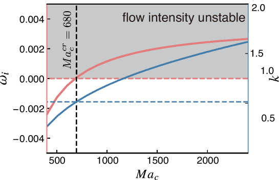
Figure 5: Influence of Marangoni number $Ma_{c}$ on Marangoni interfacial instability with $Sc=30$, $Ca=1$, $\zeta_{\mu}=1$ and $\zeta_{D}=0.2$. When $Ma_{c}$ exceeds the critical value of $Ma_{c}^{cr}=680$, the growth rate $\omega_{i}$ (red line) becomes positive, indicating flow-intensity instability (gray region), with the corresponding most unstable wave number $k^{cr}=1.015$ (blue line).

Borcia & Bestehorn (2003), Kovalchuk & Vollhardt (2006), and Lopez De La Cruz et al. (2021) have highlighted the significance of the critical Marangoni number ($Ma^{cr}_{c}$), and Marangoni flow instability arises only when the $Ma_{c}>Ma_{c}^{cr}$. To calculate the existence of $Ma^{cr}_{c}$, we varied $Ma_{c}$ under fixed parameters ($Sc=30$, $Ca=1$, $\zeta_{\mu}=1$, $\zeta_{D}=0.2$) and determined the corresponding wavenumber $k$ associated with the maximum growth rate $\omega_{i}$ at each $Ma_{c}$ value, as depicted in the figure 5. Instability is observed solely when $Ma_{c}$ surpasses $Ma^{cr}_{c}$ ($Ma^{cr}_{c}\approx 680$), with the critical wavenumber $k^{cr}$ identified as 1.015. Notably, $\zeta_{D}=0.2$ is merely one of the conditions for system instability, highlighting the requirement for the $Ma_{c}$ number to exceed $Ma^{cr}_{c}$ to manifest instability in the system.

In the following sections, we apply the DNS method to investigate the dynamic coupling process of multiple fields, aiming to gain insights into various phenomena. Specifically, we examine the self-amplification of the perturbation-triggered Marangoni interfacial flow in two flow-intensity-unstable cases (sec. 5) and the oscillation behaviour of decaying Marangoni interfacial flow in two flow-intensity-stable cases (sec. 6) by individually varying $\zeta_{\mu}$ and $\zeta_{D}$.

5 Self-Amplification of the Triggered Marangoni Interfacial Flow

Based on the DNS data, we can gain insight into the evolving process of multiple fields during the development of Marangoni flow. Without sacrificing generality, we focus on two unstable cases of $\zeta_{\mu}=10$ (#$15^{a}$ in Table 2) and $\zeta_{D}=0.2$ (#$17^{b}$ in Table 2).

5.1 Strengthening flow intensity with a viscosity ratio

When the viscosity of phase $\phi_{\text{u}}$ is ten times greater than that of phase $\phi_{\text{d}}$, indicated by the viscosity ratio $\zeta_{\mu}=10$, solute transfers from the highly viscous phase to the less viscous phase while maintaining identical diffusivity ($\zeta_{D}=1$). The remaining physical parameter are set as follows: $Sc=30,Ma_{c}=1200$, and $Ca=1$. The calculated positive energy growth rate $\omega_{i}$ indicates an increase in flow intensity. In figures 6, we present various fields at three different moments ($t^{*}=5000$, 8560, and $9500$), including the solute concentration $c^{*}$ (figs. 6($a$)), the squared velocity magnitude $\boldsymbol{u}^{*}\cdot\boldsymbol{u}^{*}$ (figs. 6($b$)), the local interfacial surface tension $\bar{\gamma}$ (figs. 6($c$)), and the local interfacial curvature $\bar{\kappa}$ (figs. 6($d$)), respectively. The definitions of $\bar{\gamma}$ and $\bar{\kappa}$ are given in Appendix A.

During the progression of the Marangoni flow, significant changes occur in solute distribution, as depicted in figs. 6($a1-a3$). The color representation indicates the intensity of solute concentration $c^{*}$, while the position of the deforming interface is delineated by a solid black line, determined as the iso-contour of $\phi_{\text{u}}=0.5$ using DNS data. Initially, the solute distribution adheres to a linear pattern along the y-axis and remains uniform along the $x$-axis. However, as time advances, the solute concentration field adjusts in accordance with the deformation of the interface. When we computed the averaged concentration field in the $x$-axis, $\langle c^{*}\rangle_{x}$, there was no discernible deviation from the linear distribution along the $y$-axis, as demonstrated in figure 6($a4$). Nevertheless, slight variations along the interface lead gradients in interfacial surface tension $\gamma^{*}$, owing to the linear relationship between $c^{*}$ and $\gamma^{*}$ described by formula (9$f$).

We derived the interfacial surface tension $\bar{\gamma}$ from DNS data using the formula

$$\bar{\gamma}=\frac{1}{\delta}{\int_{\phi_{\text{b}}=\delta_{cr}}^{\phi_{\text{b}}=1-\delta_{cr}}\gamma^{*}\mathrm{d}y^{*}},$$ (21)

where the truncation error $\delta_{cr}$ is set as 0.05. The calculated $\bar{\gamma}$ are depicted in figures 6b1-b3, confirming the growth of the gradients. It exhibits periodicity along the interface, with the repeated wavelength $\ell=2\pi/k$ corresponding to the wavelength of the most unstable mode at wavenumber $k$. In our simulation, the smallest recognized wavenumber, $k_{min}=0.2$, is determined by the size of the periodic computational domain. Thus, in this scenario, the repeated wavelength equals $\ell=10\pi$ since the mode with the wavenumber of $k=0.2$ is identified as the most unstable mode, as shown in figure 4c. Consequently, when the periodic gradients emerge, they drive solutal Marangoni interfacial flows, and the lateral extent of the convection roll is $5\pi$, half the repeated wavelength $\ell$. This phenomenon is illustrated in figure 6c1, where the flow pattern is delineated by solid lines with arrows, and indeed, the convection roll spans half the size of the simulation domain.

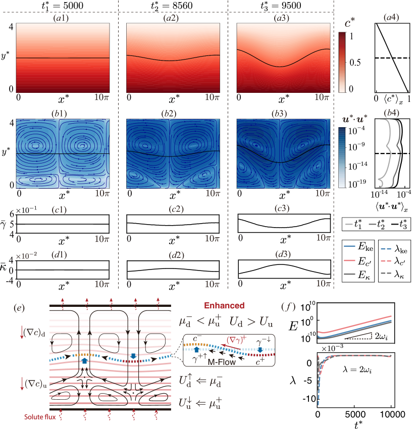
Figure 6: Self-amplification of triggered Marangoni interfacial flow when solute transfers out of a higher viscous layer ($\zeta_{\mu}=10$ and $\zeta_{D}=1$), under conditions $Sc=30,Ma_{c}=1200$, and $Ca=1$ (case $\#15$ in Table 2). DNS results at three different time instances, $t^{*}=5000,8650,$ and $9500$, are depicted as snapshots of ($a$) solute concentration field $c^{*}$, ($b$) kinetic energy field $\boldsymbol{u}^{*}\cdot\boldsymbol{u}^{*}$, ($c$) interfacial surface tension $\bar{\gamma}$, and ($d$) interfacial curvature $\bar{\kappa}$. The black solid lines in the numerical snapshots denote the interface position at $\phi_{\text{u}}=0.5$, and the dark blue lines with arrows represent streamlines. Panels ($a4$) and ($b4$) show the evolution of the $x$-direction averaged value of the concentration filed $\langle c^{*}\rangle_{x}$ and kinetic energy $\langle\boldsymbol{u}^{*}\cdot\boldsymbol{u}^{*}\rangle_{x}$. Panel ($e$) illustrates the self-amplification mechanism where interfacial deformation contributes. Panel ($f$) depicts the temporal evolution of defined total energy measures, including solute distribution energy $E_{\text{ke}}$ (blue solid line), kinetic energy $E_{c^{\prime}}$ (red solid line), and interfacial energy $E_{\kappa}$ (gray solid line), along with the corresponding growth rates $\lambda_{\text{ke}},\lambda_{c^{\prime}},\lambda_{\kappa}$ (dashed lines), which are aligned with their linear analysis predictions $2\omega_{i}$. Refer to Movie 1 and Movie 2.

When calculating the averaged velocity squared in the $x$-axis, $\langle\boldsymbol{u}^{*}\cdot\boldsymbol{u}^{*}\rangle_{x}$, we observed a consistent asymmetry in flow intensity with respect to the interface throughout the progression, as shown in figure 6($b$4). The flow intensity in phase $\phi_{\text{d}}$ surpasses than in phase $\phi_{\text{u}}$ (i.e., $U_{\text{d}}>U_{\text{u}}$) due to the lower viscosity of $\phi_{\text{d}}$ (Govindarajan & Sahu, 2014). Consequently, the stagnant point of the convection rolls shifts away from the interface towards the $\phi_{\text{u}}$ side with higher viscosity, leading to interfacial deformation as evidenced by figure 6($b1-b2$) and illustrated in figure 6($e$).

The interfacial deformation amplifies the surface local concentration gradients and the flow intensity. As sketched in the insert of figure 6($e$), the interfacial surface tension causes the Marangoni flow (M-Flow) to move from the red interfacial segment ($\gamma^{-}$) towards the orange part ($\gamma^{+}$). The red interfacial segment bends towards phase $\phi_{\text{u}}$, resulting in an increase of the local concentration by $c^{+}$ and a reduction in the local surface tension ($\gamma^{-\downarrow}$), while the bending of the orange interfacial segment towards phase $\phi_{\text{d}}$ decreases the local concentration by $c^{-}$ and increases the local surface tension ($\gamma^{+\uparrow}$). These two factors collectively contribute to the increase of the interfacial gradient at the interface, i.e., $(\nabla\gamma)^{+}$, as evidenced by the calculated $\bar{\gamma}$ in figures 6($c1-c3$). Therefore, the interfacial deformation plays a key role in strengthening the flow effect (refer to Movie 1 and Movie 2). It is worth noting that the opposite deformation leads to a decay flow effect, which will be discussed in Section 6.1.

As the flow intensity increases, the interface undergoes continued deformation and curvature, as evidenced by figures 6($b3$). Eventually, the less viscous convection rolls exert pressure against the highly viscous convection rolls until they separate the less viscous convection rolls apart and come into touch with the solid surface (refer to Movie SI-1). The evolving flow structures ultimately impose limitations on our program’s ability to further simulate the process.

The enhancement mechanism for the Marangoni interfacial flow described above is obscure in the studies that assume a non-deformation interface (Sternling & Scriven, 1959). In our simulation, there is a monotonic increase in the local interfacial curvature $\bar{\kappa}$ throughout the progression, as illustrated in fig. 6($d1-d3$). The calculation of $\bar{\kappa}$ from DNS data was based on the formula (Brackbill et al., 1992; Popinet, 2018)

$$\bar{\kappa}=\frac{\partial^{2}\bar{h}}{\partial x^{*2}}\Big{/}{\left({1+\frac{\partial\bar{h}}{\partial x^{*}}}\right)^{3/2}},$$ (22)

where the height function $\bar{h}(x)$ is obtained by fitting the order parameter $\phi$ within the interface region to a hyperbolic tangent function (refer to Appendix for the details).

To comprehensively showcase the temporal evolution of the solute concentration field, velocity field, and interfacial deformation, we correspondingly defined the three total energy measures: solute distribution energy $E_{c^{\prime}}$, kinetic energy $E_{\text{ke}}$, and interfacial energy $E_{\kappa}$, given by

$$E_{c^{\prime}}=\int_{l_{x}}\int_{l_{y}}c^{\prime 2}\mathrm{d}y^{*}\mathrm{d}x^{*},\quad E_{\text{ke}}=\int_{l_{x}}\int_{l_{y}}\boldsymbol{u}^{\prime}\cdot\boldsymbol{u}^{\prime}\mathrm{d}y^{*}\mathrm{d}x^{*},\quad E_{\kappa}={\int_{l_{x}}\bar{\kappa}^{2}\mathrm{d}x^{*}},$$ (23)

and represented as an energy set $E=(E_{c^{\prime}},E_{\text{ke}},E_{\kappa})$. Here, $\boldsymbol{u}^{\prime}=\boldsymbol{u}^{*}$ due to the base state of the velocity field being $\boldsymbol{U}^{b}=\boldsymbol{0}$ in the simulation. Figure 6($f$) illustrates the evolution of the total energy set $E$, where all three defined total energies exhibit a monotonic increase, following the same slope. This consistency is further confirmed by calculating the growth rates $\lambda=(\lambda_{c^{\prime}}$, $\lambda_{\text{ke}}$, $\lambda_{\kappa}$) for each type of total energy, as also depicted in figure 6($f$). Notably, the slope of the energy growth curve is equal to $2\omega_{i}$, which means $\lambda=2\omega_{i}$. This alignment highlights the early-stage consistency between linear and nonlinear (DNS) results. Further discussion on the correspondence of the growth rates between $E_{\kappa}$ and $E_{\text{ke}}$ (or $E_{c^{\prime}}$) is provided in Section 5.3.

5.2 Strengthening flow intensity with a diffusivity ratio

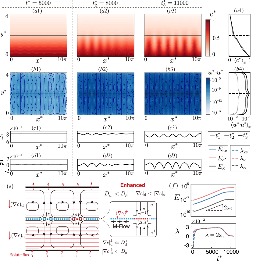
Figure 7: Self-amplification of triggered Marangoni interfacial flow when solute transfers out of a less diffusive layer ($\zeta_{D}=0.2$ and $\zeta_{\mu}=1$), under conditions $Sc=30,Ma_{c}=1200$, and $Ca=1$ (case $\#17$ in Table 2). Panels ($a-d$) depict snapshots of solute concentration field $c^{*}$, kinetic energy field $\boldsymbol{u}^{*}\cdot\boldsymbol{u}^{*}$, interfacial surface tension $\bar{\gamma}$, and interfacial curvature $\bar{\kappa}$, at three different time instances ($t^{*}=5000,8000,$ and $11000$). Panel ($e$) illustrates the self-amplification mechanism where the inequality of solute variation on the interface’s two sides contributes. Panel ($f$) depicts the temporal evolution of defined total energy set $E=(E_{\text{ke}},E_{c^{\prime}},E_{\kappa})$ and corresponding growth rate sets $\lambda=(\lambda_{\text{ke}},\lambda_{c^{\prime}},\lambda_{\kappa})$, which are aligned with linear predictions of their growth rates $2\omega_{i}$ at the early stage. The notations and conventions used here are consistent with those in figure 6. Refer to Movie 3 and Movie 4.

Strengthening Marangoni interfacial flows also occur when solute transfers from a phase with low diffusivity to a phase with high diffusivity, indicated by a diffusivity ratio $\zeta_{D}=0.2$, while both phases have identical viscosity ($\zeta_{\mu}=1$). The remaining physical parameter are set as $Sc=30,Ma_{c}=1200$, and $Ca=1$, corresponding to unstable case #$17^{b}$ in Table 2. Accordingly, we present various fields and results in figures 7, following the same order and approach as figures 6 for comparison and discussion.

Unlike the previous case with $\zeta_{\mu}=10$, where the interfacial deformation is observable, in the current scenario with identical viscosities, the interfacial deformation is negligible, as indicated by numerical snapshots at three different moments ($t^{*}=5000$, $8000$, and $11000$) in figures 7($a1-a3$), even though the large deformable interface was permitted in the nonlinear simulation. The symmetry in flow intensity with respect to the interface is consistent (figs. 7($b1-b3$)) due to the identical viscosity of the phases, as demonstrated by calculating $\langle\boldsymbol{u}^{*}\cdot\boldsymbol{u}^{*}\rangle_{x}$ in figure 7($b4$). As the progression advances, the stagnant points of convection rolls persist at the interface. Meanwhile, the size of the convection rolls converges to $5\pi/6$, which is half the repeated wavelength of the most unstable mode with a wavenumber of $k=1.2$.

In this scenario, the key to the enhancement mechanism lies in the unequal convective variation of solute concentration at the two sides of the interface. Phase $\phi_{\text{d}}$, downstream of the diffusion flux, has higher diffusivity, resulting in a more uniform solute distribution compared to the opposing side, as evidenced by the numerical snapshots in figures 7($a1-a3$). Additionally, the solute concentration distribution along $y$-axis on this side is less steep than the other (i.e., $|\nabla c|_{\text{d}}<|\nabla c|_{\text{u}}$), as indicated by the calculated $\langle c^{*}\rangle_{x}$ in figure 7($a4$) and illustrated in figure 7($e$). There exists an analytical solution for the uneven solute distribution caused by $\zeta_{D}\neq 1$, as given by the equation (2.3). It is solely attributable to pure diffusion, without convective effects. The alignment observed at the early stage ($t_{1}^{*}$) contrasts with the deviation witnessed at the late stage ($t_{3}^{*}$), illustrating how the convective effect gradually influences the concentration distribution of the system.

Upon the formation of perturbation-triggered Marangoni flow, as sketched in the insert of figure 7($e$), the interfacial Marangoni flow (M-Flow) moves away from the red interfacial segment ($\gamma^{-}$). Circular convective flows towards the red interfacial segment induce movement of dilute solute solution from the solid surfaces to the interface on the phase $\phi_{\text{d}}$ side and concentrated solute solution to the interface on the phase $\phi_{\text{u}}$ side (figs. 7($c1$)). However, the reduction of solute concentration on the phase $\phi_{\text{d}}$ side ($c^{-}$) is much smaller than the increment on the phase $\phi_{\text{u}}$ side ($c^{+}$), owing to the relatively uniform solute distribution on the phase $\phi_{\text{d}}$ side, i.e., $|\nabla c|_{\text{d}}<|\nabla c|_{\text{u}}$. Consequently, the two side convective flows collectively increase the local concentration $(\Delta c)^{+}$ and the corresponding surface tension gradients $(\nabla\gamma)^{+}$, as evidenced by the calculated $\bar{\gamma}$ in figures 7($c1-c3$). Therefore, the concentration gradients direction and their magnitude difference between two phases respond to strengthening flow effect (refer to Movie 3 and Movie 4). The opposite concentration gradient arrangement leads to a decay flow effect, which will be discussed in Section 6.2.

Eventually, the solute distribution pattern corresponding to the convection rolls is observable on the phase $\phi_{\text{u}}$ side with the relative low diffusivity (fig. 7$a3$). By calculating the local interfacial curvature $\bar{\kappa}$, we observe that the stable configuration of the interface is not flat but alternatively curved with a curvature of approximately $10^{-4}$. Comparatively, the curvature in figure 7$d3$ is merely one hundredth of that in figure 6$d3$. In previous literature, Sternling & Scriven (1959) and Kovalchuk & Vollhardt (2006) found and summarized that $\zeta_{\mu}>1$ and $\zeta_{D}<1$ would both lead to instability, but the significant differences between the two instabilities have not been elucidated. We illustrate the distinct characteristics of the three physical fields ($c^{*}$, $\boldsymbol{u}^{*}\cdot\boldsymbol{u}^{*}$, and $\bar{\kappa}$) by selecting two cases ($\zeta_{\mu}=10$ and $\zeta_{D}=0.5$), particularly emphasizing that as the energy grows linearly, the nonlinear effects on the system are not identical.

The calculated temporal evolutions of the energy set $(E_{c^{\prime}},E_{\text{ke}},E_{\kappa})$ reveal that the onset of the converging energy set coincides with the development of the alternatively curved interface. During the early stage ($t^{*}<7000$), all three total energies increase linearly at an identical growth rate $\lambda$, which closely matches the value obtained from the linear stability analysis $2\omega_{i}$, as depicted in figure 7$f$. However, following the formation of the alternatively curved interface (figs. 7$c3$ and $d3$), $\lambda$ gradually diminishes to a smaller value (fig. 7f). Ultimately, the system undergoes a supercritical bifurcation after the linear development, confirming the significant impact of nonlinear effects on the stability of the system (Kovalchuk & Vollhardt, 2008).

5.3 Interfacial evolution

From figure 6($f$) and figure 7($f$), it is found that the growth rate $\lambda$ of $E_{\kappa}$ is same to $E_{c^{\prime}}$ and $E_{\text{ke}}$. Here we perform a theoretical derivation to obtain the growth rate of $E_{\kappa}$. For the linearized phase field, the phase field variable $\phi_{\text{u}}$ can be decomposed as $\phi_{\text{u}}^{b}(y^{*})+\phi_{\text{u}}^{\prime}(x^{*},y^{*},t^{*})$, then

$$\phi_{\text{u}}^{\prime}(x^{*},y^{*},t^{*})=\tilde{\phi}_{\text{u}}(y^{*})e^{ikx^{*}-i\omega t^{*}}+c.c.=e^{\omega_{i}t^{*}}\tilde{\tilde{\phi}}_{\text{u}}(x^{*},y^{*},t^{*}).$$ (24)

Note that $\tilde{\tilde{\phi}}_{\text{u}}$ is a function of $t^{*}$, but this time variation only affects the rapid oscillation, instead of the slow growth of the disturbance amplitude. From the sec.2.1, the normal vector $\boldsymbol{n}_{\text{u}}$ can be expressed as,

$$\boldsymbol{n}_{\text{u}}=\frac{\nabla\phi_{\text{u}}}{|\nabla\phi_{\text{u}}|}=\frac{\nabla\phi_{\text{u}}^{b}+e^{\omega_{i}t^{*}}\tilde{\tilde{\phi}}_{\text{u}}}{|\nabla\phi_{\text{u}}^{b}+e^{\omega_{i}t^{*}}\tilde{\tilde{\phi}}_{\text{u}}|}\approx\frac{\nabla\phi_{\text{u}}^{b}+e^{\omega_{i}t^{*}}\tilde{\tilde{\phi}}_{\text{u}}}{|\nabla\phi_{\text{u}}^{b}|}=\frac{\nabla\phi_{\text{u}}^{b}}{|\nabla\phi_{\text{u}}^{b}|}+e^{\omega_{i}t^{*}}\frac{\tilde{\tilde{\phi}}_{\text{u}}}{|\nabla\phi_{\text{u}}^{b}|}.$$ (25)

where we know that during the initial linear phase, $\nabla\phi_{\text{u}^{b}}\gg e^{\omega_{i}t^{*}}\nabla\tilde{\tilde{\phi}}_{\text{u}}$, so we can ignore $e^{\omega_{i}t^{*}}\nabla\tilde{\tilde{\phi}}_{\text{u}}$ in the denominator. But we should not ignore that in the numerator as we are examining the initial growth. Thus, we have

$$\kappa_{\text{u}}=-\nabla\cdot\boldsymbol{n}_{\text{u}}\approx-\nabla\cdot\left(\frac{\nabla\phi_{\text{u}}^{b}}{|\nabla\phi_{\text{u}}^{b}|}\right)-e^{\omega_{i}t^{*}}\nabla\cdot\left(\frac{\tilde{\tilde{\phi}}_{\text{u}}}{|\nabla\phi_{\text{u}}^{b}|}\right).$$ (26)

For present case, $-\nabla\cdot\left(\frac{\nabla\phi_{\text{u}}^{b}}{|\nabla\phi_{\text{u}}^{b}|}\right)=-\nabla\cdot\boldsymbol{e}_{y}=0$. Then,$\kappa_{\text{u}}\approx-e^{\omega_{i}t^{*}}\nabla\cdot\left(\frac{\tilde{\tilde{\phi}}_{\text{u}}}{|\nabla\phi_{\text{u}}^{b}|}\right)$. If we take the square of it,

$$\kappa_{\text{u}}^{2}\approx e^{2\omega_{i}t^{*}}\left[\nabla\cdot\left(\frac{\tilde{\tilde{\phi}}_{\text{u}}}{|\nabla\phi_{\text{u}}^{b}|}\right)\right]^{2}.$$ (27)

where $e^{2\omega_{i}t^{*}}$ indicates that it will grow at the same rate as the $c^{\prime 2}$ and $\boldsymbol{u}^{*}\cdot\boldsymbol{u}^{*}$ in the linear stage because of $2\omega_{i}=\lambda$. And $\left[\nabla\cdot\left(\frac{\tilde{\tilde{\phi}}_{\text{u}}}{|\nabla\phi_{\text{u}}^{b}|}\right)\right]^{2}$ only affects the oscillation due to $\tilde{\tilde{\phi}}_{\text{u}}$. Through this simple derivation, we demonstrate that $\lambda$ of $E_{\kappa}$ is the same as $E_{c^{\prime}}$ and $E_{\text{ke}}$.

6 Decaying Marangoni Interfacial Flow and Oscillation

Flow oscillation presents itself as an interesting characteristic of hydrodynamic instability observed during the decay of Marangoni flow. The parameter analysis conducted in the section 4 has revealed a sub-regime of oscillating flow within the stable Marangoni flow regime, as outlined in Table 2. In this section, we investigate two typical cases of oscillation, namely $\zeta_{\mu}=0.5$ and $\zeta_{D}=5$ (corresponding to the cases #$11^{c}$ and #$20^{d}$ in Table 2), aiming to gain insight into the development of these oscillations.

6.1 Decaying flow intensity and oscillation with a viscosity ratio

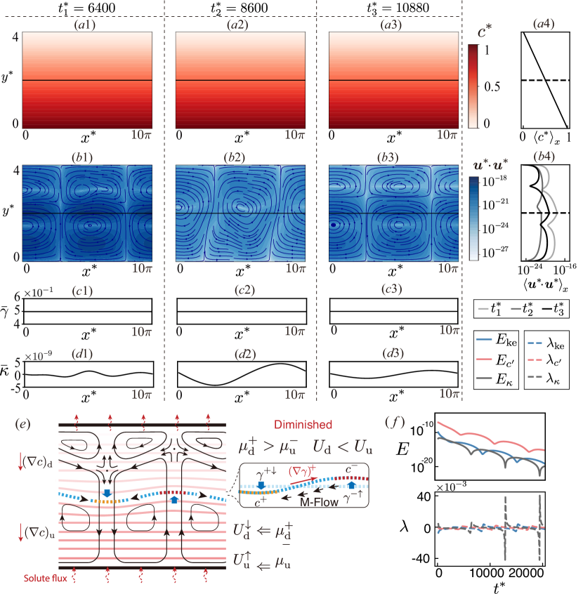
Figure 8: Decay of triggered Marangoni interfacial flow when solute transfers out of a less viscous layer ($\zeta_{\mu}=0.5$ and $\zeta_{D}=1$), under conditions $Sc=30,Ma_{c}=1200$, and $Ca=1$ (case $\#11$ in Table 2). Panels ($a-d$) depict snapshots of solute concentration field $c^{*}$, kinetic energy field $\boldsymbol{u}^{*}\cdot\boldsymbol{u}^{*}$, interfacial surface tension $\bar{\gamma}$, and interfacial curvature $\bar{\kappa}$, at three different time instances ($t^{*}=6400,8600,$ and $10880$). Panel ($e$) illustrates the decaying mechanism where the interfacial deformation contributes. Panel ($f$) depicts the temporal evolution of defined total energy set $E=(E_{\text{ke}},E_{c^{\prime}},E_{\kappa})$ and corresponding growth rate sets $\lambda=(\lambda_{\text{ke}},\lambda_{c^{\prime}},\lambda_{\kappa})$, showing an oscillatory decay. The notations and conventions used here are consistent with those in figure 6. Refer to Movie 5 and Movie 6.

For comparative analysis, we present various fields and results in figure 8, following the same order and approach applied in figures 6. Here, the solute transfers out of a less viscous phase $\phi_{\text{u}}$ ($\zeta_{\mu}=0.5$), while both phases maintain identical diffusivity. We found that the interfacial flow triggered by the solute perturbation remains un-amplified, and the influence of decay flow fields on the diffusion process proves to be negligible, as depicted in figures 8$a$ and $b$. The solute distribution $\langle c^{*}\rangle_{x}$ persists linearly along the $y$-axis (fig. 8$a4$), while the averaged velocity intensity $\langle\boldsymbol{u}^{*}\cdot\boldsymbol{u}^{*}\rangle_{x}$ evolves over time (fig. 8$b4$). Additionally, along the interface there is no observable solute gradients, and the interfacial surface tension gradients $\bar{\gamma}$ (fig. 8$c$) and the corresponding interfacial curvature $\bar{\kappa}$ (fig. 8$d$) are relatively small compared to the unstable cases (figs. 6$cd$).

In contract to previously discussed unstable case, here the flow intensity in phase $\phi_{\text{u}}$ surpasses than in phase $\phi_{\text{d}}$ (i.e., $U_{\text{d}}<U_{\text{u}}$) due to the higher viscosity of phase $\phi_{\text{d}}$. Once the interfacial flow is triggered and forms two rows of convective rolls, the stagnant points emerge within the highly viscous phase $\phi_{\text{d}}$, as demonstrated in figures 8$b$1. However, interfacial deformation affects the solute distribution along the interface by decaying the induced Marangoni interfacial flow, as illustrated in figure 8$e$. In the insert of figure 8$e$, the interfacial surface tension causes the Marangoni flow (M-Flow) to move from the red interfacial segment ($\gamma^{-}$) towards the orange part ($\gamma^{+}$). Consequently, the deformation of the red segment towards phase $\phi_{\text{d}}$ results in a decrease in local concentration ($c^{-}$) and an increase in local surface tension $(\gamma^{-\uparrow})$, whereas the orange interfacial segment experiences an increase in concentration ($c^{+}$) and a decrease in surface tension $(\gamma^{+\downarrow})$. These changes collectively reduce the existing surface tension gradient, thereby leading to the decay of the triggered flow (refer to Movie 5 and Movie 6).

The flow intensity in Figure 8$b$ is negligible compared to that in Figure 6$b$, despite the continuous decrease in the convection flow rate, as indicated by the calculated total kinetic energy $E_{\text{ke}}$ in Figure 6$f$. During this period, the stagnant points gradually shift towards the interface, and the interface becomes correspondingly flat, as confirmed by calculating $E_{\bar{\kappa}}$ and $E_{c^{\prime}}$(fig. 6$f$). It is noteworthy that, even though in the stable case the growth rates of all modes are negative, the mode with the wavenumber of $k=0.2$ has the smallest decay rate (fig. 4$c$), corresponding to the repeated wavelength of $\ell=10\pi$.

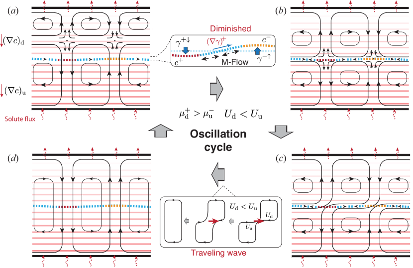
Figure 9: Illustration of oscillatory decay mechanism when solute transfers out of a less viscous layer with identical diffusivity ($\zeta_{\mu}=0.5$ and $\zeta_{D}=1$). During one oscillation cycle: ($a$) Two rows of convection rolls form with stagnant points in the higher viscous layer. ($b$) The convection rolls gradually become symmetric with respect to the interface. ($c$) Coalescence occurs between two diagonal convection rolls, leading to a distorted convection structure. ($d$) The irregular convection structures reshape into convection rolls, associated with a traveling wave on the interface. The instability of one row of convection rolls triggers the emergence of a second row in the higher viscous layer, initiating the subsequent oscillation cycle. Refer to Movie 6.

We observed that the oscillation of flow pattern during the decay is a distinctive characteristic, which is also evident from $\omega_{r}\neq 0$ at $\zeta_{\mu}=0.5$ in figure 4$d$. The mechanism, as illustrated in Figure 9, involves the convection rolls pattern becoming symmetric with respect the interface (from fig. 9$a$ to fig. 9$b$), followed by the viscosity contrast between two phases triggering another instability, leading to the coalescence between two diagonal convection rolls. The merging-up of the two diagonal convection rolls results in one distorted convection structure. Subsequently, the distorted convection structures reshape into a row of convection rolls (Govindarajan & Sahu, 2014), as illustrated in the insert between figure 9$c$ and figure 9$d$. As a consequence, the flattened interface rapidly curves. This process is reflected in figure 8$f$ by the sudden increase in interfacial energy $E_{\bar{\kappa}}$ ($t*=6400$) and subsequently diminishing in kinetic energy $E_{\text{ke}}$ ($6400<t*<8600$). This reshaping motion of the distorted convection roll is associated with the formation of a traveling wave.

The two-row pattern of convection rolls undergoes a repeating cycle of the previously described processes (Movie 6), ultimately leading to the oscillation of the flow pattern. The one-row pattern of convective rolls is unable to sustain due to the asymmetric distribution of viscosity with respect to the interface. Thus, the gradual shifting of the roll centers towards the low viscous phase initiates to the formation of a new row of convection rolls from the high viscous boundary, thereby initiating another cycle. During the oscillation, the repeated wavelength maintains $\ell=10\pi$, consistent with results that only mode $k=0.2$ has the smallest decay growth rate $\omega_{i}$ in figure 4$c$.

6.2 Decaying flow intensity and oscillation with a diffusivity ratio

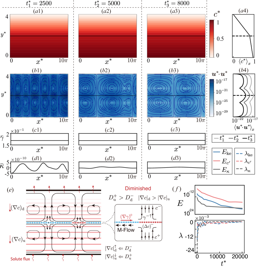
Figure 10: Decay of triggered Marangoni interfacial flow when solute transfers out of a highly diffusive layer ($\zeta_{D}=5$ and $\zeta_{\mu}=1$), under conditions $Sc=30,Ma_{c}=1200$, and $Ca=1$ (case $\#20$ in Table 2). Panels ($a-d$) depict snapshots of solute concentration field $c^{*}$, kinetic energy field $\boldsymbol{u}^{*}\cdot\boldsymbol{u}^{*}$, interfacial surface tension $\bar{\gamma}$, and interfacial curvature $\bar{\kappa}$, at three different time instances ($t^{*}=2500,5000,$ and $8000$). Panel ($e$) illustrates the decaying mechanism where the interfacial deformation contributes. Panel ($f$) depicts the temporal evolution of defined total energy set $E=(E_{\text{ke}},E_{c^{\prime}},E_{\kappa})$ and corresponding growth rate sets $\lambda=(\lambda_{\text{ke}},\lambda_{c^{\prime}},\lambda_{\kappa})$, showing an fluctuating growth rates during the early stages ($t^{*}>5000$). The notations and conventions used here are consistent with those in figure 6. Refer to Movie 7 and Movie 8.

The Marangoni flows triggered by solute perturbation also decay when the solute transfers out of a high diffusivity phase $\phi_{\text{u}}$ ($\zeta_{D}=5$), while both phases maintain identical viscosity, as depicted in figure 10$a$ and $b$. We found that the difference in diffusivity between the two phases results in a steeper solute distribution along the $y$-axis on the low diffusivity phase $\phi_{\text{d}}$ side (i.e., $|\nabla c|_{\text{d}}>|\nabla c|_{\text{u}}$), as represented by the solute concentration fields snapshots in figures 10$a1$-$a3$. The diffusion process dominates the solute distribution over the decaying convective flow, thus the calculated $\langle c^{*}\rangle_{x}$ persists linearly along the $y$-axis (fig. 10$a4$), contrasting with the convection-induced variation observed in the unstable case (fig. 7$a4$). The hydrodynamic symmetry is maintained with respect to the interface during the evolution of the flow field, as demonstrated by the numerical snapshots of streamlines at different moments (figs. 10$b$1-$b3$) and the calculated $\langle\boldsymbol{u}^{*}\cdot\boldsymbol{u}^{*}\rangle_{x}$ (fig. 10$b4$). The interfacial surface tension gradients $\bar{\gamma}$ (fig. 10$c$) and the corresponding interfacial curvature $\bar{\kappa}$ (fig. 10$d$) are not only invisible compared to those in the unstable case (fig. 7$cd$) but also relatively smaller than those in the stable case with a viscosity ratio (fig. 8$cd$).

The unequal variation of solute concentration at the two sides of the interface not only contributes to the strengthening of the Marangoni interfacial flow but also to the decaying case with a diffusivity ratio. As illustrated in figure 10$e$, the triggered Marangoni flows (M-Flow) transport liquids away from the red interfacial segment, while convective flows bring some fresh liquids to replenish it. On the $\phi_{\text{d}}$ phase side, it is refilled by the dilute solute solution ($c^{-}$), while the $\phi_{\text{u}}$ side is refilled by the concentrated solute solution ($c^{+}$). Due to the higher diffusivity in phase $\phi_{\text{u}}$, there are gentle solute gradients along the y-axis compared to phase $\phi_{\text{d}}$, i.e., $|\nabla c|_{\text{d}}>|\nabla c|_{\text{u}}$. The balanced convective flows ($\zeta_{\mu}=1$) from the two sides collectively result in a reduction of solute concentration $(\Delta c)^{-}$ and the corresponding decrease in surface tension gradient $(\nabla\gamma)^{-}$. Thus, the raised interfacial flows self-weaken, leading to a decaying flow effect (refer to Movie 7 and Movie 8).

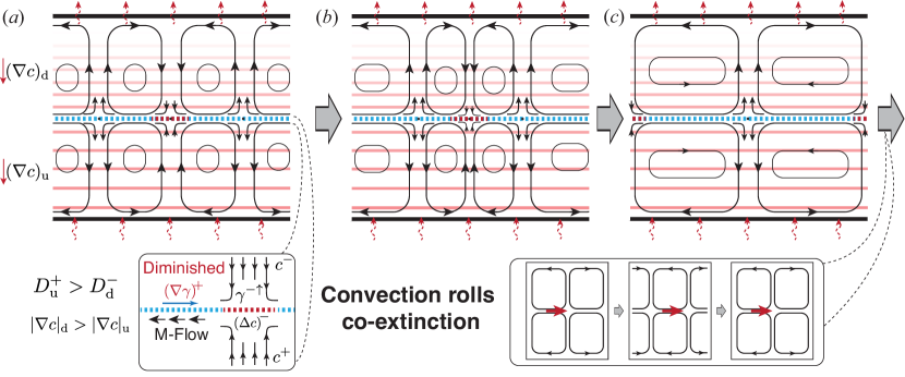
Figure 11: Illustration of oscillatory decay mechanisms when solute transfers out of a highly diffusive layer ($\zeta_{D}=5$ and $\zeta_{\mu}=1$). The oscillation arises from the co-extinction of adjacent convection rolls: ($a$) Two rows of convection rolls form symmetrically with respect to the interface. ($b$) Reduced flow intensity towards the interface (red interfacial segment) causes the adjacent convention rolls to shrink. ($c$) Consequently, the pair of shrinking convection rolls co-extinct, resulting in an oscillation of the flow pattern. Ultimately, the remaining convection rolls move uniformly along one direction. Refer to Movie 8.

When we analyzed the evolution of energy components $E_{\text{ke}}$, $E_{c^{\prime}}$, and $E_{\kappa}$ represented in blue, red, and gray color respectively in figure 10f, we confirmed the decaying flow effect. The calculated growth rates of these energies fluctuate, especially during the early stages ($t^{*}>5000$), reflecting the repeated diminishing of the triggered flow as described previously. We numerically observed that each diminishing event results in the co-extinction of adjacent convection rolls, as illustrated in figure 11. Since the flow at the stagnation point in the red interfacial region weakens (fig. 11$a$), the two adjacent convective rolls are correspondingly depressed, leading to the reduction in roll size (fig. 11$b$). Eventually, the two convection rolls cancel out, and the size of the remaining convection rolls increases (Movie 8). This process repeats, associated with the fluctuating decaying rate of the of the total energy set, and concludes when the size of convection rolls matches the wavelength ($\ell=10\pi$) of the slowest decaying mode ($k=0.2$, refer to fig. 4$e$). Subsequently, the residual convection rolls continue to decay but with movement in one direction (fig. 11$c$), likely initiated by the inertia from the last cancellation process.

It worthy noting that the proposed DNS method enabled us to gain insight of the processes and propose the corresponding mechanisms to the different types of oscillations, although the oscillation and evolution of convection roll have been reported and investigated in some work  Schwarzenberger et al. (2014); Kovalchuk & Vollhardt (2006); Shin et al. (2016)

7 Conclusions

In summary, our study involved both analytical and numerical investigations into Marangoni interfacial instability triggered in a two-liquid-layer system with constant solute transfer across the liquid interface. We developed a numerical model based on phase-field method and rigorously verified and validated it by comparing the calculations results with linear stability analysis. The investigated physical parameter space spans $Sc\in[0.2,200]$, $Ma_{c}\in[10,2000]$, $Ca\in[0.01,1]$, $\zeta_{\mu}\in[0.1,10]$, and $\zeta_{D}\in[0.1,10]$.

Through direct numerical simulations that incorporated interfacial deformation and nonlinearity, we investigated how the viscosity ratio $\zeta_{\mu}$ and diffusivity ratio $\zeta_{D}$ of two liquid layers influence the hydrodynamic stability of the system. We identified two key characteristics of Marangoni hydrodynamic instability: the strengthening of the perturbation-triggered Marangoni interfacial flow (in the flow-intensity-unstable case) and the oscillation of flow patterns during the decaying of the triggered Marangoni interfacial flow (in the flow-intensity-stable case). Our findings revealed that perturbation-triggered Marangoni interfacial flows are amplified and sustained under specific conditions, such as solute transfer out of a higher viscous layer with identical diffusivity ($\zeta_{\mu}>1$ and $\zeta_{D}=1$), or out of a less diffusive layer with identical viscosity ($\zeta_{D}<1$ and $\zeta_{\mu}=1$). These results align with those reported by Sternling & Scriven (1959).

Furthermore, our deformable-interface-incorporated model highlighted that interfacial deformation and unequal solute variation at the interface’s two sides contribute to Marangoni hydrodynamic instability in cases affected by viscosity ratio and diffusivity ratio, respectively. In the flow-intensity-unstable case, the nonlinear growth rate exhibited early-stage consistency between linear and nonlinear results, ultimately reaching a state of nonlinear saturation. Additionally, we numerically observed traveling waves in the flow-intensity-stable case, which are associated with the morphological evolution of convection rolls.

Based on these insights, we have proposed corresponding instability mechanisms, which were substantiated and confirmed by analyzing the evolution and interaction of multiple fields, including the solute concentration field, flow field, interfacial surface tension field, and interfacial curvature field. Through detailed examination and correlation of these fields, we established a comprehensive understanding of the mechanisms underlying Marangoni hydrodynamic instability in the context of varying viscosity and diffusivity ratios between the two liquid layers.

Appendix A List of definitions

In the section 5 and 6, the additional definitions are given as follows. The average distribution of solute concentration $c^{*}$ in $x$-direction $\langle c^{*}\rangle_{x}$ is defined as,

$$\langle c^{*}\rangle_{x}=\frac{1}{l_{x}}\int_{0}^{l_{x}}c^{*}\mathrm{d}x^{*}.$$ (28)

It shows the average concentration of solutes at each horizontal position. Similarly, the average flow intensity at each horizontal position is represented by $\langle\boldsymbol{u}^{*}\cdot\boldsymbol{u}^{*}\rangle_{x}$. And it is defined as

$$\langle\boldsymbol{u}^{*}\cdot\boldsymbol{u}^{*}\rangle_{x}=\frac{1}{l_{x}}\int_{0}^{l_{x}}\boldsymbol{u}^{*}\cdot\boldsymbol{u}^{*}\mathrm{d}x^{*}.$$ (29)

The total energy set contains solute distribution energy $E_{c^{\prime}}$, kinetic energy $E_{\text{ke}}$, and interfacial energy $E_{\kappa}$. They are given by

$$E_{c^{\prime}}=\int_{l_{x}}\int_{l_{y}}c^{\prime 2}\mathrm{d}y^{*}\mathrm{d}x^{*},\quad E_{\text{ke}}=\int_{l_{x}}\int_{l_{y}}\boldsymbol{u}^{\prime}\cdot\boldsymbol{u}^{\prime}\mathrm{d}y^{*}\mathrm{d}x^{*},\quad E_{\kappa}={\int_{l_{x}}\bar{\kappa}^{2}\mathrm{d}x^{*}},$$ (30)

respectively. Here, $\boldsymbol{u}^{\prime}=\boldsymbol{u}^{*}$ due to the base state of the velocity field being $\boldsymbol{U}^{b}=\boldsymbol{0}$. The growth rates of the energy set are calculated via

$$\lambda_{c^{\prime}}=\frac{\ln\left[{E}_{c^{\prime}}(t^{*}+\mathrm{\Delta}t)/{E}_{c^{\prime}}(t^{*})\right]}{\mathrm{\Delta}t},$$ (31a)

$$\lambda_{\text{ke}}=\frac{\ln\left[{E}_{\text{ke}}(t^{*}+\mathrm{\Delta}t)/{E}_{\text{ke}}(t^{*})\right]}{\mathrm{\Delta}t},$$ (31b)

$$\lambda_{\kappa}=\frac{\ln\left[{E}_{\kappa}(t^{*}+\mathrm{\Delta}t)/{E}_{\kappa}(t^{*})\right]}{\mathrm{\Delta}t}.$$ (31c)

Appendix B List of physical symbols

English symbols
$a_{i}$	Lagrange multipliers in the phase field equations of $\phi_{i}$ phase
$A$	a coefficient in the weight function of surface tension $SF$
$B$	a relation between excess interfacial free energy and bulk energy
$c$	solute concentration
$c^{*}$	dimensionless solute concentration
$c^{\prime}$	perturbation of solute concentration
$\tilde{c}$	eigenfunction of solute concentration
$C^{b}$	base state of solute concentration
$D_{i}$	solute diffusivity of $\phi_{i}$ phase
$D$	solute diffusivity of whole space
$D^{*}$	dimensionless solute diffusivity
$\hat{E}_{\text{ke}}$	total kinetic energy of DNS results in spectral space
$E$	total energy set
$E_{\text{ke}}$	kinetic energy
$E_{c^{\prime}}$	solute distribution energy
$E_{\kappa}$	interfacial energy
$\mathcal{E}$	free energy functional
$G_{c}$	gradient of solute concentration
$\bar{h}$	a hyperbolic tangent function of fitting $\phi$
$\boldsymbol{I}_{i}$	Identic matrix in $phi_{i}$ phase
$k$	wavenumber
$L$	characteristic length
$l_{x}$, $l_{y}$	computational physical region in $x$ and $y$ direction
$\ell$	wavelength
$M_{\phi}$	mobility of phase field
$N_{x}$, $N_{y}$	number of grids in $x$ and $y$ direction for DNS
$\boldsymbol{n}_{i}$	normal vector of $\phi_{i}$ phase
$p$	pressure
$p^{*}$	dimensionless pressure
$p^{\prime}$	perturbation of pressure
$P$	characteristic pressure
$P^{b}$	base state of pressure
$\tilde{p}$	eigenfunction of pressure
$\boldsymbol{SF}$	surface tension
$t$	time
$\hat{T}$	time period of energy oscillation in spectral space
$t^{*}$	dimensionless time
$\boldsymbol{u}$	velocity vector
$\boldsymbol{u}^{*}$	dimensionless velocity vector
$\boldsymbol{u}^{\prime}$	perturbation of velocity vector
$\tilde{\boldsymbol{u}}$	eigenfunction of velocity vector
$\hat{u}$, $\hat{v}$	the velocity field of DNS results in spectral space
$U$	characteristic velocity
$\boldsymbol{U}^{b}$	base state of velocity vector
${u}^{\prime},{v}^{\prime}$	perturbation of velocity in $x$ and $y$ direction
$\tilde{u},\tilde{v}$	eigenfunction of velocity in $x$ and $y$ direction
$W$	weight function in surface tension
$W^{*}$	dimensionless form of weight function in surface tension
$\boldsymbol{x}$	position vector of Cartesian coordinate system
$\boldsymbol{x}^{*}$	dimensionless position vector
$x$, $y$	dimensional length in horizontal, vertical direction
$x^{*}$, $y^{*}$	dimensionless length in horizontal, vertical direction
Greek symbols
$\beta$	linear relation between solute and surface tension coefficient
$\gamma$	surface tension coefficient
$\gamma_{0}$	surface tension coefficient without solute contaminated
$\gamma^{*}$	dimensionless surface tension coefficient
$\Gamma^{b}$	base state of surface tension coefficient
$\delta$	interfacial region
$\delta_{cr}$	truncated interfacial region
$\epsilon_{1}$	coefficient of the excess free energy of interfacial region
$\epsilon_{2}$	coefficient of the double-well potential function of the bulk energy
$\zeta_{\mu}$	viscosity ratio between $\phi_{1}$ and $\phi_{2}$
$\zeta_{D}$	diffusivity ratio between $\phi_{1}$ and $\phi_{2}$
$\zeta_{h}$	liquid pool depth ratio between $\phi_{1}$ and $\phi_{2}$
$\kappa$	curvature
$\kappa^{*}$	dimensionless curvature
$\kappa_{i}$	curvature of $\phi_{i}$
$\bar{\kappa}$	the average curvature of the interface
$\lambda$	energies growth rate in DNS
$\lambda_{\text{ke}}$	growth rate of kinetic energy in DNS
$\lambda_{c^{\prime}}$	growth rate of solute distribution energy in DNS
$\lambda_{\kappa}$	growth rate of interfacial energy in DNS
$\mu_{i}$	viscosity of $\phi_{i}$ phase
$\mu_{i}^{*}$	dimensionless viscosity of $\phi_{i}$ phase
$\rho_{i}$	density of $\phi_{i}$ phase
$\rho_{i}^{*}$	dimensionless density of $\phi_{i}$ phase
$\phi_{i}$	order parameter of phase field
$\phi_{eq}$	equilibrium state of phase field
$\phi_{i}^{b}$	base state of $\phi_{i}$
$\phi_{i}^{\prime}$	perturbation of $\phi_{i}$
$\tilde{\phi}_{i}$	eigenfunction of $\phi_{i}$
$\tilde{\tilde{\phi}}_{i}$	eigenfunction of $\phi_{i}$ affected by rapid oscillation
$\omega$	complex frequency of energy
$\omega_{i}$	linear growth rate of energy
$\omega_{r}$	oscillation frequency of energy
Dimensional numbers
$Ca$	Capillary number
$Ma_{\phi}$	Marangoni number of phase field
$Ma_{c}$	Marangoni number of solute
$Sc$	Schmidt number
$Re$	Reynolds number
Superscripts
∗	dimensionless form
b	base state
′	perturbation
cr	critical value
Subscripts
${}_{\text{u}}$	the upstream phase of solute diffusion
${}_{\text{d}}$	the downstream phase of solute diffusion
${}_{\text{ke}}$	kinetic energy
${}_{{c^{\prime}}}$	energy of perturbation solute concentration
κ	interfacial energy

References

- Aihara et al. (2019) Aihara, Shintaro, Takaki, Tomohiro & Takada, Naoki 2019 Multi-phase-field modeling using a conservative allen–cahn equation for multiphase flow. Computers & Fluids 178, 141–151.
- Banerjee et al. (2016) Banerjee, Anirudha, Williams, Ian, Azevedo, Rodrigo Nery, Helgeson, Matthew E & Squires, Todd M 2016 Soluto-inertial phenomena: Designing long-range, long-lasting, surface-specific interactions in suspensions. Proceedings of the National Academy of Sciences 113 (31), 8612–8617.
- Baumgartner et al. (2022) Baumgartner, Dieter A., Shiri, Samira, Sinha, Shayandev, Karpitschka, Stefan & Cira, Nate J. 2022 Marangoni spreading and contracting three-component droplets on completely wetting surfaces. Proceedings of the National Academy of Sciences 119 (19), e2120432119.
- Borcia & Bestehorn (2003) Borcia, Rodica & Bestehorn, Michael 2003 Phase-field model for Marangoni convection in liquid-gas systems with a deformable interface. Physical Review E 67 (6), 066307.
- Brackbill et al. (1992) Brackbill, J.U, Kothe, D.B & Zemach, C 1992 A continuum method for modeling surface tension. Journal of Computational Physics 100 (2), 335–354.
- Brennecke & Maginn (2001) Brennecke, Joan F. & Maginn, Edward J. 2001 Ionic liquids: Innovative fluids for chemical processing. AIChE Journal 47 (11), 2384–2389.
- Chao et al. (2022) Chao, Youchuang, Ramírez-Soto, Olinka, Bahr, Christian & Karpitschka, Stefan 2022 How liquid–liquid phase separation induces active spreading. Proceedings of the National Academy of Sciences 119 (30), e2203510119.
- Chiu & Lin (2011) Chiu, Pao-Hsiung & Lin, Yan-Ting 2011 A conservative phase field method for solving incompressible two-phase flows. Journal of Computational Physics 230 (1), 185–204.
- Cira et al. (2015) Cira, Nate J, Benusiglio, Adrien & Prakash, Manu 2015 Vapour-mediated sensing and motility in two-component droplets. Nature 519 (7544), 446–450.
- Degen et al. (1998) Degen, Michael M, Colovas, Peter W & Andereck, C David 1998 Time-dependent patterns in the two-layer rayleigh-bénard system. Physical Review E 57 (6), 6647.
- Demont et al. (2023) Demont, T.H.B., Stoter, S.K.F. & Van Brummelen, E.H. 2023 Numerical investigation of the sharp-interface limit of the Navier-Stokes-Cahn-Hilliard equations. Journal of Fluid Mechanics 970, A24.
- Dwivedi et al. (2022) Dwivedi, Prateek, Pillai, Dipin & Mangal, Rahul 2022 Self-propelled swimming droplets. Current Opinion in Colloid & Interface Science p. 101614.
- Frenkel & Halpern (2002) Frenkel, Alexander L. & Halpern, David 2002 Stokes-flow instability due to interfacial surfactant. Physics of Fluids 14 (7), L45–L48.
- Frenkel & Halpern (2017) Frenkel, Alexander L. & Halpern, David 2017 Surfactant and gravity dependent instability of two-layer Couette flows and its nonlinear saturation. Journal of Fluid Mechanics 826, 158–204.
- Govindarajan & Sahu (2014) Govindarajan, Rama & Sahu, Kirti Chandra 2014 Instabilities in viscosity-stratified flow. Annual Review of Fluid Mechanics 46 (Volume 46, 2014), 331–353.
- Guo et al. (2021) Guo, Wei, Kinghorn, Andrew B, Zhang, Yage, Li, Qingchuan, Poonam, Aditi Dey, Tanner, Julian A & Shum, Ho Cheung 2021 Non-associative phase separation in an evaporating droplet as a model for prebiotic compartmentalization. Nature Communications 12 (1), 3194.
- Halpern & Frenkel (2003) Halpern, David & Frenkel, Alexander L. 2003 Destabilization of a creeping flow by interfacial surfactant: linear theory extended to all wavenumbers. Journal of Fluid Mechanics 485, 191–220.
- Hu et al. (2021) Hu, Kai-Xin, Zhao, Cheng-Zhuo, Zhang, Shao-Neng & Chen, Qi-Sheng 2021 Instabilities of thermocapillary liquid layers with two free surfaces. International Journal of Heat and Mass Transfer 173, 121217.
- Izri et al. (2014) Izri, Ziane, Van Der Linden, Marjolein N, Michelin, Sébastien & Dauchot, Olivier 2014 Self-propulsion of pure water droplets by spontaneous marangoni-stress-driven motion. Physical review letters 113 (24), 248302.
- Jacqmin (1999) Jacqmin, David 1999 Calculation of Two-Phase Navier Stokes Flows Using Phase-Field Modeling. Journal of Computational Physics 155 (1), 96–127.
- Jin et al. (2017) Jin, Chenyu, Krüger, Carsten & Maass, Corinna C 2017 Chemotaxis and autochemotaxis of self-propelling droplet swimmers. Proceedings of the National Academy of Sciences 114 (20), 5089–5094.
- Kalliadasis et al. (2003) Kalliadasis, Serafim, Kiyashko, Alla & Demekhin, E. A. 2003 Marangoni instability of a thin liquid film heated from below by a local heat source. Journal of Fluid Mechanics 475, 377–408.
- Kalogirou (2018) Kalogirou, Anna 2018 Instability of two-layer film flows due to the interacting effects of surfactants, inertia, and gravity. Physics of Fluids 30 (3), 030707.
- Kalogirou & Blyth (2020) Kalogirou, A. & Blyth, M. G. 2020 Nonlinear dynamics of two-layer channel flow with soluble surfactant below or above the critical micelle concentration. Journal of Fluid Mechanics 900, A7.
- Kalogirou et al. (2016) Kalogirou, A., Cîmpeanu, R., Keaveny, E. E. & Papageorgiou, D. T. 2016 Capturing nonlinear dynamics of two-fluid Couette flows with asymptotic models. Journal of Fluid Mechanics 806, R1.
- Khossravi & Connors (1993) Khossravi, Davar & Connors, Kenneth A. 1993 Solvent effects on chemical processes. 3. Surface tension of binary aqueous organic solvents. Journal of Solution Chemistry 22 (4), 321–330.
- Kim (2012) Kim, Junseok 2012 Phase-Field Models for Multi-Component Fluid Flows. Communications in Computational Physics 12 (3), 613–661.
- Kovalchuk & Vollhardt (2006) Kovalchuk, N.M. & Vollhardt, D. 2006 Marangoni instability and spontaneous non-linear oscillations produced at liquid interfaces by surfactant transfer. Advances in Colloid and Interface Science 120 (1-3), 1–31.
- Kovalchuk & Vollhardt (2008) Kovalchuk, N. M. & Vollhardt, D. 2008 Oscillation of Interfacial Tension Produced by Transfer of Nonionic Surfactant through the Liquid/Liquid Interface. The Journal of Physical Chemistry C 112 (24), 9016–9022.
- Lee & Kim (2015) Lee, Hyun Geun & Kim, Junseok 2015 An efficient numerical method for simulating multiphase flows using a diffuse interface model. Physica A: Statistical Mechanics and its Applications 423, 33–50.
- Levich & Krylov (1969) Levich, VG & Krylov, VS 1969 Surface-tension-driven phenomena. Annual review of fluid mechanics 1 (1), 293–316.
- Li et al. (2021) Li, Yanshen, Diddens, Christian, Prosperetti, Andrea & Lohse, Detlef 2021 Marangoni Instability of a Drop in a Stably Stratified Liquid. Physical Review Letters 126 (12), 124502.
- Li et al. (2023) Li, Yitan, Pahlavan, Amir A, Chen, Yuguang, Liu, Song, Li, Yan, Stone, Howard A & Granick, Steve 2023 Oil-on-water droplets faceted and stabilized by vortex halos in the subphase. Proceedings of the National Academy of Sciences 120 (4), e2214657120.
- Lohse & Zhang (2020) Lohse, Detlef & Zhang, Xuehua 2020 Physicochemical hydrodynamics of droplets out of equilibrium. Nature Reviews Physics 2 (8), 426–443.
- Lopez De La Cruz et al. (2021) Lopez De La Cruz, Ricardo Arturo, Diddens, Christian, Zhang, Xuehua & Lohse, Detlef 2021 Marangoni instability triggered by selective evaporation of a binary liquid inside a Hele-Shaw cell. Journal of Fluid Mechanics 923, A16.
- Lyu et al. (2021) Lyu, Sijia, Tan, Huanshu, Wakata, Yuki, Yang, Xianjun, Law, Chung K, Lohse, Detlef & Sun, Chao 2021 On explosive boiling of a multicomponent leidenfrost drop. Proceedings of the National Academy of Sciences 118 (2), e2016107118.
- Maass et al. (2016) Maass, Corinna C, Krüger, Carsten, Herminghaus, Stephan & Bahr, Christian 2016 Swimming droplets. Annual Review of Condensed Matter Physics 7, 171–193.
- Manikantan & Squires (2020) Manikantan, Harishankar & Squires, Todd M 2020 Surfactant dynamics: hidden variables controlling fluid flows. Journal of fluid mechanics 892, P1.
- Mao et al. (2023) Mao, Qi, Yang, Qing-Jun, Liu, Yu & Cao, Wang 2023 Experimental and numerical study of droplet formation with Marangoni instability. Chemical Engineering Science 268, 118369.
- May et al. (2022) May, Alexander, Hartmann, Johannes & Hardt, Steffen 2022 Phase separation in evaporating all-aqueous sessile drops. Soft Matter 18 (34), 6313–6317.
- Mokbel et al. (2017) Mokbel, Marcel, Schwarzenberger, Karin, Eckert, Kerstin & Aland, Sebastian 2017 The influence of interface curvature on solutal Marangoni convection in the Hele-Shaw cell. International Journal of Heat and Mass Transfer 115, 1064–1073.
- Nejati et al. (2015) Nejati, Iman, Dietzel, Mathias & Hardt, Steffen 2015 Conjugated liquid layers driven by the short-wavelength bénard–marangoni instability: experiment and numerical simulation. Journal of Fluid Mechanics 783, 46–71.
- Oertel (2004) Oertel, Herbert, ed. 2004 Biofluid Mechanics of Blood Circulation, pp. 615–654. New York, NY: Springer New York.
- Oron et al. (1995) Oron, A, Deissler, R.J & Duh, J.C 1995 Marangoni instability in a liquid sheet. Advances in Space Research 16 (7), 83–86.
- Pearson (1958) Pearson, J. R. A. 1958 On convection cells induced by surface tension. Journal of Fluid Mechanics 4 (5), 489–500.
- Picardo et al. (2016) Picardo, Jason R., Radhakrishna, T. G. & Pushpavanam, S. 2016 Solutal marangoni instability in layered two-phase flows. Journal of Fluid Mechanics 793, 280–315.
- Popinet (2018) Popinet, Stéphane 2018 Numerical Models of Surface Tension. Annual Review of Fluid Mechanics 50 (1), 49–75.
- Schwarzenberger et al. (2014) Schwarzenberger, Karin, Köllner, Thomas, Linde, Hartmut, Boeck, Thomas, Odenbach, Stefan & Eckert, Kerstin 2014 Pattern formation and mass transfer under stationary solutal Marangoni instability. Advances in Colloid and Interface Science 206, 344–371.
- Shim (2022) Shim, Suin 2022 Diffusiophoresis, diffusioosmosis, and microfluidics: surface-flow-driven phenomena in the presence of flow. Chemical Reviews 122 (7), 6986–7009.
- Shin et al. (2016) Shin, Sangwoo, Jacobi, Ian & Stone, Howard A. 2016 Bénard-Marangoni instability driven by moisture absorption. EPL (Europhysics Letters) 113 (2), 24002.
- Slavtchev & Mendes (2004) Slavtchev, S. & Mendes, M.A. 2004 Marangoni instability in binary liquid–liquid systems. International Journal of Heat and Mass Transfer 47 (14-16), 3269–3278.
- Snell & Helliwell (2005) Snell, Edward H & Helliwell, John R 2005 Macromolecular crystallization in microgravity. Reports on Progress in Physics 68 (4), 799–853.
- Sternling & Scriven (1959) Sternling, C. V. & Scriven, L. E. 1959 Interfacial turbulence: Hydrodynamic instability and the marangoni effect. AIChE Journal 5 (4), 514–523.
- Tan et al. (2021) Tan, Huanshu, Banerjee, Anirudha, Shi, Nan, Tang, Xiaoyu, Abdel-Fattah, Amr & Squires, Todd M 2021 A two-step strategy for delivering particles to targets hidden within microfabricated porous media. Science advances 7 (33), eabh0638.
- Tan et al. (2016) Tan, Huanshu, Diddens, Christian, Lv, Pengyu, Kuerten, Johannes GM, Zhang, Xuehua & Lohse, Detlef 2016 Evaporation-triggered microdroplet nucleation and the four life phases of an evaporating ouzo drop. Proceedings of the National Academy of Sciences 113 (31), 8642–8647.
- Tan et al. (2019a) Tan, Huanshu, Diddens, Christian, Mohammed, Ali Akash, Li, Junyi, Versluis, Michel, Zhang, Xuehua & Lohse, Detlef 2019a Microdroplet nucleation by dissolution of a multicomponent drop in a host liquid. Journal of fluid mechanics 870, 217–246.
- Tan et al. (2023) Tan, Huanshu, Lohse, Detlef & Zhang, Xuehua 2023 Self-lubricating drops. Current Opinion in Colloid & Interface Science p. 101744.
- Tan et al. (2019b) Tan, Huanshu, Wooh, Sanghyuk, Butt, Hans-Jürgen, Zhang, Xuehua & Lohse, Detlef 2019b Porous supraparticle assembly through self-lubricating evaporating colloidal ouzo drops. Nature communications 10 (1), 478.
- Velegol et al. (2016) Velegol, Darrell, Garg, Astha, Guha, Rajarshi, Kar, Abhishek & Kumar, Manish 2016 Origins of concentration gradients for diffusiophoresis. Soft matter 12 (21), 4686–4703.
- Wang et al. (2022) Wang, Zhenying, Orejon, Daniel, Takata, Yasuyuki & Sefiane, Khellil 2022 Wetting and evaporation of multicomponent droplets. Physics Reports 960, 1–37.
- Wei (2005) Wei, Hsien-Hung 2005 On the flow-induced marangoni instability due to the presence of surfactant. Journal of Fluid Mechanics 544, 173–200.
- Wei (2006) Wei, Hsien-Hung 2006 Shear-flow and thermocapillary interfacial instabilities in a two-layer viscous flow. Physics of Fluids 18 (6), 064109.