Rate Analysis of Coupled Distributed Stochastic Approximation for Misspecified Optimization

Abstract

We consider an $n$ agents distributed optimization problem with imperfect information characterized in a parametric sense, where the unknown parameter can be solved by a distinct distributed parameter learning problem. Though each agent only has access to its local parameter learning and computational problem, they mean to collaboratively minimize the average of their local cost functions. To address the special optimization problem, we propose a coupled distributed stochastic approximation algorithm, in which every agent updates the current beliefs of its unknown parameter and decision variable by stochastic approximation method; then averages the beliefs and decision variables of its neighbors over network in consensus protocol. Our interest lies in the convergence analysis of this algorithm. We quantitatively characterize the factors that affect the algorithm performance, and prove that the mean-squared error of the decision variable is bounded by $\mathcal{O}(\frac{1}{nk})+\mathcal{O}\left(\frac{1}{\sqrt{n}(1-\rho_{w})}\right)\frac{1}{k^{1.5}}+\mathcal{O}\big{(}\frac{1}{(1-\rho_{w})^{2}}\big{)}\frac{1}{k^{2}}$, where $k$ is the iteration count and $(1-\rho_{w})$ is the spectral gap of the network weighted adjacency matrix. It reveals that the network connectivity characterized by $(1-\rho_{w})$ only influences the high order of convergence rate, while the domain rate still acts the same as the centralized algorithm. In addition, we analyze that the transient iteration needed for reaching its dominant rate $\mathcal{O}(\frac{1}{nk})$ is $\mathcal{O}(\frac{n}{(1-\rho_{w})^{2}})$. Numerical experiments are carried out to demonstrate the theoretical results by taking different CPUs as agents, which is more applicable to real-world distributed scenarios.

1 Introduction

In recent years, distributed optimization has drawn much research attention in various fields including economic dispatch[1, 2], smart grids [3, 4, 5], automatic controls[6, 7, 8] and machine learning [9, 10]. In distributed scenarios, each agent only preserves its local information, while they can exchange information with others over a connected network to cooperatively minimize the average of all agents’ cost functions [11, 12]. There are several approaches for resolving distributed optimization problems such as (primary) consensus-based, duality-based, and constraint exchange methods, where the primal approaches characterized by gradient-based algorithms have attracted the most research attention due to their satisfactory performance and well-scalable nature[13]. The distributed dual approaches based on Lagrange method regularly use dual decomposition like the alternating direction method of multipliers (ADMM)[14]. Constraint exchange method is another prevalent scheme where the information exchanged by agents amounts to constraints[15].

However, among various formulations in distributed optimization, a crucial assumption is that we need precise objective functions (or problem information), i.e., all parameters in the model are precisely known. Yet in many economic and engineering problems, parameters of the functions are unknown but we may have access to observations that can aid in resolving this misspecification. For example, in the Markowitz profile problem, it is routinely assumed that the expectation or covariance matrices associated with a collection of stocks are accurately available, but in reality, it needs empirical estimates via past data[16].

This paper is devoted to proposing distributed algorithms for resolving optimization problems with parametric misspecification, and quantitatively characterizing the influence of network properties, the heterogeneity of agents, initial states, etc. on the algorithm performance. This work is primarily centered around conducting a comprehensive theoretical analysis of convergence. We begin by initiating the problem formulation.

1.1 Problem Formulation

In this article, we consider a static misspecified distributed optimization problem defined as follows:

$$\mathcal{C}_{x}(\theta_{*}):\qquad\min_{x\in\mathbb{R}^{p}}f(x,\theta_{*})=\frac{1}{n}\sum\nolimits_{i=1}^{n}f_{i}(x,\theta_{*}),$$ (1)

where $f_{i}(x,\theta_{*})\triangleq\mathbb{E}[\tilde{f}_{i}(x,\theta,\xi_{i})]$ is the local cost function only accessible for agent $i\in\mathcal{N}\triangleq\{1,2,...,n\}$. Suppose that for any $i\in\mathcal{N}$, $\xi_{i}:\Omega_{x}\rightarrow\mathbb{R}^{d}$ are mutually independent random variables defined on a probability space $(\Omega_{x},\mathcal{F}_{x},\mathbb{P}_{x})$. Here, $\theta_{*}\in\mathbb{R}^{q}$ denotes the unknown parameter, which is a solution to a distinct convex problem.

$$\mathcal{L}_{\theta}:\qquad\min_{\theta\in\mathbb{R}^{q}}h(\theta)=\frac{1}{n}\sum\nolimits_{i=1}^{n}h_{i}(\theta),$$ (2)

where $h_{i}(\theta)\triangleq\mathbb{E}[\tilde{h}_{i}(\theta,\zeta_{i})]$ is the local parameter learning function only accessible for agent $i\in\mathcal{N}$, and for any $i\in\mathcal{N}$, $\zeta_{i}:\Omega_{\theta}\rightarrow\mathbb{R}^{m}$ are mutually independent random variables defined on a probability space $(\Omega_{\theta},\mathcal{F}_{\theta},\mathbb{P}_{\theta})$. Problems in the form eq. 1 and eq. 2 jointly formulate an unknown coupled distributed optimization scheme consisting of both computational problem and learning problem, where the learning problem is independent of the computational one. We have depicted the problem setting in fig. 1.

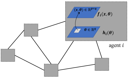
Figure 1: The problem setup: a connected network of communicating agents, where each agent preserving a local learning problem $h_{i}$ and computational problem $f_{i}$ correlated with $h_{i}$ through the unknown parameter $\theta$, while they cooperate to solve the distributed coupled optimization problem.

1.2 Prior Work

We now give a review of prior work for resolving optimization problems with unknown parameters.

Robust optimization approach. Robust optimization considers the optimization problem where the parameter $\theta$ is unavailable but one can have access to its uncertainty set, say $\mathcal{U}_{\theta}$[17]. The key idea is to optimize against the worst-case realization within this set, i.e.,

$$\min_{x\in\mathbb{R}^{p}}\max_{\theta\in\mathcal{U}_{\theta}}f(x,\theta).$$

Robust optimization is shown to be a useful technique in the resolution of problems arising from control, design, and optimization [18]. However, it usually produces conservative solutions and sometimes is intractable when poor set $\mathcal{U}_{\theta}$ is chosen (e.g. the set is given by unexplicit systems of non-convex inequalities)[19].

Stochastic optimization. Unlike robust optimization, in a stochastic optimization scenario one may obtain statistical or distributional information about the unknown parameter. For example, $\theta$ follows a probability distribution $\mathcal{D}$[20], the optimal solution is gained by minimizing the expectation of cost functions,

$$\min_{x\in\mathbb{R}^{p}}\mathbb{E}_{\theta\sim\mathcal{D}}[f(x,\theta)].$$

Stochastic optimization has been widely investigated in telecommunication, finance and machine learning [21]. In the scenario of a multi-agent network dealing with large datasets, stochastic optimization has become popular since it is challenging to calculate the exact gradient while the stochastic gradient is much easier to obtain. A key shortcoming in using stochastic optimization models for resolving optimization problems with unknown parameters lies in that it needs the distribution of $\theta$, which might be a stringent requirement when the available data for estimating is limited or noisy. In such cases, the resulting distribution estimates may be unreliable or biased, leading to suboptimal solutions or even infeasible solutions[22]. Alternatively, suppose that $\theta_{*}$ can be learnt by a suitably defined estimation problem, then it brings about the following approach.

Data-driven learning approach. As data availability reaches hitherto unseen in recent years, we can use data-driven approaches to lessen or even eliminate the impact of model uncertainty. For example, the model parameter $\theta$ can be obtained by solving a suitably defined learning problem $l(\theta)$ (see e.g., [23]),

$$\min_{x\in\mathbb{R}^{p}}\left\{f(x,\theta_{*}):\theta_{*}\in\mathop{\arg\min}\limits_{\theta\in\mathbb{R}^{q}}l(\theta)\right\}.$$ (3)

Computational evidence in portfolio management and queueing confirm that data-driven sets significantly outperform traditional robust optimization techniques[19].

A natural question is whether this problem could be solved in a sequential method, i.e., first accomplish estimating $\theta_{*}$ with high accuracy and then solve the core computational optimization problem with the achieved estimation $\hat{\theta}$. However, they have some disadvantages discussed in [23, 24, 25]: on the one hand, the large-scale parameter learning problem will lead to long time waiting for solving the original problem. On the other hand, this scheme provides an approximate solution $\hat{\theta}$, then the corrupt error might propagates into the computational problem. As such, sequential methods cannot provide asymptotically accurate convergence. Therefore, an alternative simultaneous approach is designed (see e.g., [23, 26]), which use observations to get an estimation $\theta_{k}$ of unknown parameters $\theta^{*}$ at each time instant $k$; then update the upper optimization problem by taking the estimated parameter $\theta_{k}$ as “true” parameter. This simultaneous approach can generate a sequence $\{(x_{k},\theta_{k})\}$ that converges to a minimizer of $f(x,\theta_{*})$ and $l(\theta)$ respectively [23].

Such data-driven learning approaches for unknown parameter has gradually attracted research attention recently. For example, the authors of [23] presented a centralized coupled stochastic optimization scheme to solve problem (3) and showed the convergence properties in regimes when the function is either strongly convex or merely convex. Then [25] extended it smooth or nonsmooth functions $f$ and presented an averaging-based subgradient approach, but it is still a centralized scheme. In addition, the authors of [24] divided the optimization problem with uncertainty into two paradigms: robust optimization and joint estimation optimization, and they exploited these two problem structures in online convex optimization and gave regret analysis under different conditions. The recent work [16] investigated the misspecified conic convex programs, and developed a centralized first-order inexact augmented Lagrangian scheme for computing the optimal solution while simultaneously learning the unknown parameters. The aforementioned work [16, 24, 23, 25] all investigated centralized methods, while there are some other work exploit distributed approaches. For example, [27] considered the distributed stochastic optimization with imperfect information, while it only showed that the generated iterates converge almost surely to the optimal solution. Though the work [28] presented a distributed problem with a composite structure consisting of an exact engineering part and an unknown personalized part, it exhibits a bounded regret under certain conditions.

1.3 Gaps and Motivation

Recalling the problem setup in section 1.1, our research falls into distributed data-driven stochastic optimization scenario. Taking into account the research that is most pertinent to this paper, the majority of previous studies have primarily concentrated on centralized inquiries (see e.g. [16, 24, 23, 25]), while the distributed schemes [27, 28] mainly investigated the asymptotic convergence. It remains unknown how to design an efficient distributed algorithm, how does the network connectivity influence the algorithm performance, and whether the rate can reach the same order as the centralized scheme? To be specific, this paper is motivated by the following gaps: (i) previous work on unknown parameter learning problems focused on the centralized scheme, the distributed data-driven stochastic approximation method is less studied; (ii) the discussion of convergence analysis especially how factors such as the number of agents, the network connectivity, and the heterogeneity of agents influence the rate of algorithm is rarely studied in details; (iii) the gap between centralized and distributed algorithm under imperfect information need to be specified, or in other words can we find the transient time when the rate of distributed algorithms reach the same order as that of the centralized scheme?

1.4 Outline and Contributions

To address these gaps, we propose a data-driven coupled distributed stochastic approximation method to resolve this special optimization problem and give a precise convergence rate analysis of our algorithm. The main contributions are summarized as follows, and the comparison with previous works is shown in table 1.

Table 1: Work comparation with previous studies

Paper	Distributed	Imperctect Information	Stochastic	Rate	Factor Influence
[24, 23, 25]	✗	✓	✗	$\mathcal{O}\left(\frac{1}{k}\right)$	✗
[29, 30]	✓	✗	✓	$\mathcal{O}\left(\frac{1}{k}\right)$	✓
[28]	✓	✓	✗	$\backslash$	✓
[27]	✓	✓	✓	$\backslash$	✗
[31]	✓	✗	✗	$\mathcal{O}\left(\frac{1}{\sqrt{k}}\right)$	✗
Our Work	✓	✓	✓	$\mathcal{O}\left(\frac{1}{k}\right)$	✓

(1) We propose a coupled distributed stochastic approximation algorithm that generates iterates {$(\boldsymbol{\mathbf{x}}(k),\boldsymbol{\mathbf{\theta}}(k))$} for the distributed stochastic optimization problem (1) with the unknown parameter learning prescribed by a separate distributed stochastic optimization problem (2). Our model framework builds upon previous research involving deterministic and stochastic gradient schemes. This is particularly relevant for certain studies where waiting for parameter learning to complete over an extended period is not feasible, or for real-world problems in which parameter learning and objective optimization are intertwined.

(2) We characterize the convergence rate of the presented algorithm that combined the distributed consensus protocol with stochastic gradient descent methods. On the one hand, we prove that the upper bound of expected consensus error for every agent decay at rate $\mathcal{O}(\frac{1}{k^{2}})$; on the other hand, we also show that the upper bounded of expected optimization error is $\mathcal{O}(\frac{1}{k})$. We then give the sublinear convergence rate and quantitatively characterize some factors affecting the convergence rate, such as the network size, spectral gap of the weighted adjacency matrix, heterogenous of individual function, and initial values. We emphasize that the mean-squared error of the decision variable is bounded by $\mathcal{O}(\frac{1}{nk})+\mathcal{O}\left(\frac{1}{\sqrt{n}(1-\rho_{w})}\right)\frac{1}{k^{1.5}}+\mathcal{O}\big{(}\frac{1}{(1-\rho_{w})^{2}}\big{)}\frac{1}{k^{2}}$, which indicates that the network connectivity characterized by $(1-\rho_{w})$ only influences the high order of convergence rate, while the domain rate $\mathcal{O}(\frac{1}{k})$ still acts the same as the centralized algorithm.

(3) We analyze the transient time $K_{T}$ for the proposed algorithm, namely, the number of iterations before the algorithm reaches its dominant rate. Specially, we show that when the iterate $k\geq K_{T}$, the dominant factor influencing the convergence rate is related to stochastic gradient descent, while for small $k<K_{T}$, the main factor influencing the convergence rate originates from the distributed average consensus method. Finally, we show that the algorithm asymptotically achieves the same network-independent convergence rate as the centralized scheme.

The paper is organized as follows. We present the algorithm and the related assumptions in section 2. In section 3, the auxiliary results supporting the convergence rate analysis is proved. Our main results are in section 4. Experimental results are implemented in section 5, while the concluding remarks are given in section 6.

Notation. All vectors in this paper are column vectors. The structure of the communication network is modeled by an undirected weighted graph $\mathcal{G}=(\mathcal{N},\mathcal{E},\mathcal{W})$ in which $\mathcal{N}=\{1,2,...,n\}$ represents the set of vertices. $\mathcal{E}\subseteq\mathcal{N}\times\mathcal{N}$ is the set of edges. $W=[w_{ij}]_{n\times n}\in\mathbb{R}^{n\times n}$ denotes the weighted adjacency matrix, $w_{ij}>0$ if and only if agent $i$ and agent $j$ are connected, $w_{ij}=w_{ji}=0$ otherwise. Each agent(vertice) has a set of neighbors $\mathcal{N}_{i}=\{j|(i,j)\in\mathcal{E}\}$. The graph is connected means for every pair of nodes $(i,j)$ there exists a path of edges that goes from $i$ to $j$. $||\cdot||$ denotes $\mathcal{L}_{2}$-norm for vectors and Euclidean norm for matrices. The optimal solution denote as ($x_{*},\theta_{*}$).

2 Algorithm and Assumptions

To solve this special optimization problem consisting of the computational problem eq. 1 and the learning problem eq. 2, we will propose a Coupled Distributed Stochastic Approximation (CDSA) Algorithm and impose some conditions for rate analysis in this section.

2.1 Algorithm Set Up

As mentioned previously, each agent $i$ only knows its local core computational function $f_{i}(x,\theta)$ and parameter learning function $h_{i}(\theta)$, while they are connected by a network $\mathcal{G}=(\mathcal{N},\mathcal{E},\mathcal{W})$ in which agents may communicate and exchange information with their neighbors $\mathcal{N}_{i}=\{j|(i,j)\in\mathcal{E}\}$. At each step $k\geq 0$, every agent $i$ holds an estimate of the decision variable and unknown parameter, denoted by $x_{i}(k)$ and $\theta_{i}(k)$, respectively. Suppose that every agent has access to a stochastic first-order oracle that can generate stochastic gradients $g_{i}(x_{i}(k),\theta_{i}(k),\xi_{i}(k))\triangleq\nabla_{x}f_{i}(x_{i}(k),\theta_{i}(k),\xi_{i}(k))$ and $\phi_{i}(\theta_{i}(k),\zeta_{i}(k))\triangleq\nabla_{\theta}h_{i}(\theta_{i}(k),\zeta_{i}(k))$ respectively (where $\xi_{i},\zeta_{i},i=1,2,...,n$ are independent random variables). Then, every agent updates its parameters through stochastic gradient descent method to obtain temporary estimates $\widetilde{x}_{i}(k)$ and $\widetilde{\theta}_{i}(k)$. Next, each agent communicates with its local neighbors and gathers temporary parameters information over a static connected network to renew the iterates $x_{i}(k+1)$ and $\theta_{i}(k+1)$ based on the consensus protocol. We summarize the pseudo-code is in algorithm 1.

Algorithm 1 Coupled Distributed Stochastic Approximation (CDSA)

  Initialization: $W=[w_{ij}]_{n\times n};(x_{i}(0),\theta_{i}(0)),\forall i\in\mathcal{N}$

  Evolution: for $k=0,1,2,...;\forall i\in\mathcal{N}$

    Compute: stochastic gradient $\phi_{i}\left(\theta_{i}(k),\zeta_{i}(k)\right)$ and $g_{i}(x_{i}(l),\theta_{i}(k),\xi_{i}(k))$

    Choose: stepsize $\alpha_{k}$ and $\gamma_{k}$ (To be introduced in section 3.3)

    Update according to the following stochastic gradient descent method.

$$\widetilde{x}_{i}(k) =x_{i}(k)-\alpha_{k}g_{i}(x_{i}(k),\theta_{i}(k),\xi_{i}(k))$$

$$\widetilde{\theta}_{i}(k) =\theta_{i}(k)-\gamma_{k}\phi_{i}\left(\theta_{i}(k),\zeta_{i}(k)\right)$$

    Gather information $\widetilde{x}_{j}(k),\widetilde{\theta}_{j}(k)$ from its neighbors $j\in\mathcal{N}_{i}$ and renew the iterates by the consensus protocol below.

$$x_{i}(k+1) =\sum\nolimits_{j\in\mathcal{N}_{i}}w_{ij}\widetilde{x}_{j}(k)$$

$$\theta_{i}(k+1) =\sum\nolimits_{j\in\mathcal{N}_{i}}w_{ij}\widetilde{\theta}_{j}(k)$$

We can rewrite Algorithm 1 in a more compact form as follows.

$$x_{i}(k+1) =\sum\nolimits_{j\in\mathcal{N}_{i}}w_{ij}(x_{j}(k)-\alpha_{k}g_{j}(x_{i}(l),\theta_{i}(k),\xi_{i}(k))),$$ (4)

$$\theta_{i}(k+1) =\sum\nolimits_{j\in\mathcal{N}_{i}}w_{ij}\left(\theta_{j}(k)-\gamma_{k}\phi_{j}\left(\theta_{i}(k),\zeta_{i}(k)\right)\right).$$ (5)

Define

$$\boldsymbol{\mathbf{x}} \triangleq[x_{1},x_{2},\cdots,x_{n}]^{T}\in\mathbb{R}^{n\times p},\boldsymbol{\mathbf{\theta}}\triangleq[\theta_{1},\theta_{2},\cdots,\theta_{n}]^{T}\in\mathbb{R}^{n\times q},$$ (6)

$$\boldsymbol{\xi} \triangleq[\xi_{1},\xi_{2},\cdots,\xi_{n}]^{T}\in\mathbb{R}^{n},~{}\boldsymbol{\zeta}\triangleq[\zeta_{1},\zeta_{2},\cdots,\zeta_{n}]^{T}\in\mathbb{R}^{n},$$ (7)

$$\mathbf{g}(\boldsymbol{\mathbf{x}},\boldsymbol{\theta},\boldsymbol{\mathbf{\xi}}) \triangleq[g_{1}(x_{1},\theta_{1},\xi_{1}),g_{2}(x_{2},\theta_{2},\xi_{2}),\cdots,g_{n}(x_{n},\theta_{n},\xi_{n})]^{T}\in\mathbb{R}^{n\times p},$$ (8)

$$\boldsymbol{\phi}(\boldsymbol{\theta},\boldsymbol{\mathbf{\zeta}}) \triangleq[\phi_{i}\left(\theta_{1},\zeta_{1}\right),\phi_{i}\left(\theta_{2},\zeta_{2}\right),\cdots,\phi_{i}\left(\theta_{n},\zeta_{n}\right)]^{T}\in\mathbb{R}^{n\times q}.$$ (9)

Then equation (4) and (5) can be reformulated in the following vector formula.

$$\boldsymbol{\mathbf{x}}(k+1) =W\left(\boldsymbol{\mathbf{x}}(k)-\alpha_{k}\mathbf{g}(\boldsymbol{\mathbf{x}}(k),\boldsymbol{\theta}(k),\boldsymbol{\mathbf{\xi}}(k))\right),$$ (10)

$$\boldsymbol{\mathbf{\theta}}(k+1) =W\left(\boldsymbol{\mathbf{\theta}}(k)-\alpha_{k}\boldsymbol{\phi}(\boldsymbol{\theta}(k),\boldsymbol{\mathbf{\zeta}}(k))\right).$$ (11)

2.2 Assumptions

In this subsection, we will specify the conditions for rate analysis of the CDSA algorithm. We need to make some assumptions about the properties of objective functions in both learning and computation metrics to get the global optimal solution. Besides, we impose some constraints on conditional first and second moments of “stochastic gradient”. Last but not least, we inherit the typical assumptions about communication networks as that of distributed algorithms.

Assumption 2.2.1 (Function properties).

(i) For every $\theta\in\mathbb{R}^{q}$, $f_{i}(x,\theta),i=1,\cdots,n$ is strongly convex and Lipschitz smooth in $x$ with constants $\mu_{x}$ and $L_{x}$, i.e.

$$(\nabla_{x}f_{i}(x^{\prime},\theta)-\nabla_{x}f_{i}(x,\theta))^{T}(x^{\prime}-x) \geq\mu_{x}||x^{\prime}-x||^{2},\forall x,x^{\prime}\in\mathbb{R}^{p},$$

$$||\nabla_{x}f_{i}(x^{\prime},\theta)-\nabla_{x}f_{i}(x,\theta)|| \leq L_{x}||x^{\prime}-x||,\forall x,x^{\prime}\in\in\mathbb{R}^{p}.$$

(ii) For every $x\in\mathbb{R}^{p}$, $f_{i}(x,\theta),i=1,\cdots,n$ is strongly convex and Lipschitz smooth in $\theta$ with constants $\mu_{\theta}$ and $L_{\theta}$ respectively, i.e.

$$(\nabla_{x}f_{i}(x,\theta^{\prime})-\nabla_{x}f_{i}(x,\theta))^{T}(\theta^{\prime}-\theta) \geq\mu_{\theta}||\theta^{\prime}-\theta||^{2},\forall\theta,\theta^{\prime}\in\mathbb{R}^{q},$$

$$||\nabla_{x}f_{i}(x,\theta^{\prime})-\nabla_{\theta}f(x,\theta)|| \leq L_{\theta}||\theta^{\prime}-\theta||,\forall\theta,\theta^{\prime}\in\mathbb{R}^{q}.$$

(iii)The learning metric $h_{i}(\theta)$ for every $i\in\{1,2,...,n\}$ is strongly convex and Lipschitz smooth with constants $\nu_{\theta}$ and $C_{\theta}$, i.e.

$$(h(\theta)-h(\theta^{\prime}))^{T}(\theta-\theta^{\prime}) \geq\nu_{\theta}||\theta-\theta^{\prime}||^{2},\forall\theta,\theta^{\prime}\in\mathbb{R}^{q},$$

$$||\nabla h(\theta)-\nabla h(\theta^{\prime})|| \leq C_{\theta}||\theta-\theta^{\prime}||,\forall\theta,\theta^{\prime}\in\mathbb{R}^{q}.$$

Strong convexity assumptions indicate that both computational problem and learning problem have a unique optimal solution $x_{*}\in\mathbb{R}^{p}$ and $\theta_{*}\in\mathbb{R}^{q}$ [32]. The Lipschitz continuity of gradient functions ensure that the gradient doesn’t change arbitrarily fast concerning the corresponding parameter vector. It is widely used in the convergence analyses of most gradient-based methods, without it, the gradient wouldn’t provide a good indicator for how far to move to decrease the objective function[32]. These assumptions are satisfied for many machine learning problems, such as logistic regression, linear regression, and support vector machine (SVM).

Next, we define a new probability space $(\mathcal{Z},\mathcal{F},\mathbb{P})$, where $\mathcal{Z}\triangleq\Omega_{x}\times\Omega_{\theta},\mathcal{F}\triangleq\mathcal{F}_{x}\times\mathcal{F}_{\theta}$ and $\mathbb{P}\triangleq\mathbb{P}_{x}\times\mathbb{P}_{\theta}$. We use $\mathcal{F}(k)$ to denote the $\sigma$-algebra generated by $\{(x_{i}(0),\theta_{i}(0)),(x_{i}(1),\theta_{i}(1)),...,(x_{i}(k),\theta_{i}(k))|i\in\mathcal{N}\}$. Then give the following assumptions related to the stochastic gradient estimator, which assume that the stochastic gradient is an unbiased estimator of the true gradient, and the variance of the stochastic gradient is restricted.

Assumption 2.2.2 (Conditional first and second moments).

For all $k\geq 0$ and $i\in\mathcal{N}$,there exist $\sigma_{x}>0,\sigma_{\theta}>0,M_{x}>0,M_{\theta}>0$, such that

$$(a)\quad\mathbb{E}_{\xi_{i}(k)}[g_{i}(x_{i}(k),\theta_{i}(k),\xi_{i}(k))|\mathcal{F}(k)]=\nabla_{x}f_{i}(x_{i}(k),\theta_{i}(k)),\quad a.s.,$$

$$(b)\quad\mathbb{E}_{\zeta_{i}(k)}[\phi_{i}(\theta_{i}(k),\zeta_{i}(k))|\mathcal{F}(k)]=\nabla h_{i}(\theta_{i}(k)),\quad a.s.,$$

$$(c)\quad\mathbb{E}_{\xi_{i}(k)}[||g_{i}(x_{i}(k),\theta_{i}(k),\xi_{i}(k))-\nabla_{x}f_{i}(x_{i}(k),\theta_{i}(k))||^{2}|\mathcal{F}(k)],$$

$$\qquad\qquad\qquad\qquad\leq\sigma_{x}^{2}+M_{x}||\nabla_{x}f_{i}(x_{i}(k),\theta_{i}(k))||^{2}\quad a.s.,$$

$$(d)\quad\mathbb{E}_{\zeta_{i}(k)}[||\phi_{i}(\theta_{i}(k),\zeta_{i}(k))-\nabla h_{i}(\theta_{i}(k))||^{2}|\mathcal{F}(k)]\leq\sigma_{\theta}^{2}+M_{\theta}||\nabla h_{i}(\theta_{i}(k))||^{2},\quad a.s.,$$

Next, we impose the connectivity condition on the graph, which indicates that after multiple rounds of communication, information can be exchanged between any two agents. This inherits the typical assumptions on consensus protocols [33].

Assumption 2.2.3 (Graph and weighted matrix).

The graph $\mathcal{G}$ is static, undirected, and connected. The weighted adjacency matrix $W$ is nonnegative and doubly stochastic, i.e.,

$$W\boldsymbol{1}=\boldsymbol{1},\boldsymbol{1}^{T}W=\boldsymbol{1}^{T}$$ (12)

where $\boldsymbol{1}$ is the vector of all ones.

Next, we state two lemmas that partially explain the practicability of algorithm 1 based on the aforementioned assumptions.

Lemma 2.2.1.

[34, Lemma 10] For any $x\in\mathbb{R}^{p}$, define $x^{+}=x-\alpha\nabla f(x)$. Suppose that $f$ is strongly convex with constant $\mu$ and its gradient function is Lipschitz continuous with constant $L$. If $\alpha\in(0,2/L)$, we then have $||x^{+}-x_{*}||\leq\lambda||x-x_{*}||,$ where $\lambda\triangleq\max(|1-\alpha\mu|,|1-\alpha L|)$.

It can be observed from the above lemma that as long as we choose a proper stepsize ($0<\alpha<2/L$), the distance to optimizer shrinks by a ratio $\lambda<1$ at each step for strongly convex and smooth functions. While the following lemma reveals that under distributed algorithm with linear iteration, the gap between the current iteration and consensus optimal solution is decreased by a ratio $\rho_{w}<1$ compared to the last iteration.

Lemma 2.2.2.

[33, Theorem 1] Let Assumption 2.2.3 hold, and $\rho_{w}$ denote the spectural norm of matrix $W-\frac{\boldsymbol{1}\boldsymbol{1}^{T}}{n}$. Thus $\rho_{w}<1$. Define $\boldsymbol{\omega}^{+}=W\boldsymbol{\omega}$ for any $\boldsymbol{\omega}\in\mathbb{R}^{n\times p}$. We then have $||\boldsymbol{\omega}^{+}-\boldsymbol{1}\bar{\omega}||\leq\rho_{w}||\boldsymbol{\omega}-\boldsymbol{1}\bar{\omega}||,$ where $\bar{\omega}\triangleq\frac{1}{n}\boldsymbol{1}^{T}\boldsymbol{\omega}$.

The aforementioned lemmas show that both the gradient descent method and distributed linear iteration can move the decision variable towards the optimal solution with linear decaying rates. Thus, our algorithm consisting of both approaches might find the optimal solution efficiently. We will rigorously prove the convergence rate of algorithm 1 in the following two sections.

3 Auxiliary Results

In this section, we will present some results to assist subsequent convergence rate analysis. We first give some preliminary bound which will be used for later proof, then present the supporting lemmas concerning recursions for expected optimization error and expected consensus error, and finally, we prove that under diminishing stepsize, the mean-squared distance between the current iterate and the optimal solution is uniformly bounded.

3.1 Preliminary Bound

For simplicity, we denote

$$\bar{x}(k)\triangleq\frac{1}{n}\sum\nolimits_{i=1}^{n} x_{i}(k),~{}\bar{\theta}(k)\triangleq\frac{1}{n}\sum\nolimits_{i=1}^{n}\theta_{i}(k),$$ (13)

$$\bar{g}(\boldsymbol{\mathbf{x}}(k),\boldsymbol{\mathbf{\theta}}(k),\boldsymbol{\mathbf{\xi}}(k)) \triangleq\frac{1}{n}\sum\nolimits_{i=1}^{n}g_{i}(x_{i}(k),\theta_{i}(k),\xi_{i}(k)),$$ (14)

$$\bar{\nabla}_{x}F(\boldsymbol{\mathbf{x}}(k),\boldsymbol{\mathbf{\theta}}(k)) \triangleq\frac{1}{n}\sum\nolimits_{i=1}^{n}\nabla_{x}f_{i}\left(x_{i}(k),\theta_{i}(k)\right).$$ (15)

We will show in the following lemma that with Assumptions 2.2.1 and 2.2.2, the conditional squared distance between the gradient $\bar{\nabla}_{x}F(\boldsymbol{\mathbf{x}}(k),\boldsymbol{\mathbf{\theta}}(k))$ and its estimate can be bounded by linear combinations of squared errors $||\boldsymbol{\mathbf{x}}(k)-\boldsymbol{1}x_{*}^{T}||^{2}$ and $||\boldsymbol{\mathbf{\theta}}(k)-\boldsymbol{1}\theta_{*}^{T}||^{2}$. For completeness, its proof is given in appendix A.

Lemma 3.1.1.

Let Assumption 2.2.1 and 2.2.2 hold. Then for any $k\geq 0$,

$$\mathbb{E}[||\bar{g}(\boldsymbol{\mathbf{x}}(k),\boldsymbol{\mathbf{\theta}}(k),\boldsymbol{\mathbf{\xi}}(k)) -\bar{\nabla}_{x}F(\boldsymbol{\mathbf{x}}(k),\boldsymbol{\mathbf{\theta}}(k))||^{2}|\mathcal{F}(k)]$$

$$\leq\frac{3M_{x}L_{x}^{2}}{n^{2}}||\boldsymbol{\mathbf{x}}(k)-\boldsymbol{1}x_{*}^{T}||^{2}+\frac{3M_{x}L_{\theta}^{2}}{n^{2}}||\boldsymbol{\mathbf{\theta}}(k)-\boldsymbol{1}\theta_{*}^{T}||^{2}+\frac{\bar{M}}{n},$$ (16)

$$\text{where}\quad\bar{M} =\frac{3M_{x}\sum\nolimits_{i=1}^{n}||\nabla_{x}f_{i}(x_{*},\theta_{*})||^{2}}{n}+\sigma_{x}^{2}.$$ (17)

The following lemma shows the gap between the gradient of objective function at the consensual points $(\bar{x}(k),\bar{\theta}(k))$, denoted by $\frac{1}{n}\sum\nolimits_{i=1}^{n}\nabla_{x}f_{i}(\bar{x}(k),\bar{\theta}(k))$, and at current iterates $\frac{1}{n}\sum\nolimits_{i=1}^{n}\nabla_{x}f_{i}(x_{i}(k),\theta_{i}(k))$ can also be bounded by linear combinations of $||\boldsymbol{\mathbf{x}}(k)-\boldsymbol{1}x_{*}^{T}||^{2}$ and $||\boldsymbol{\mathbf{\theta}}(k)-\boldsymbol{1}\theta_{*}^{T}||^{2}$. The precise proof is in appendix B.

Lemma 3.1.2.

Let Assumption 2.2.1 hold. Then for any $k\geq 0$,

$$||\nabla_{x}f(\bar{x}(k),\bar{\theta}(k))-\bar{\nabla}_{x}F(\boldsymbol{\mathbf{x}}(k),\boldsymbol{\mathbf{\theta}}(k))||\leq\frac{L_{x}}{\sqrt{n}}||\boldsymbol{\mathbf{x}}(k)-\boldsymbol{1}\bar{x}(k)^{T}||+\frac{L_{\theta}}{\sqrt{n}}||\boldsymbol{\mathbf{\theta}}(k)-\boldsymbol{1}\bar{\theta}(k)^{T}||.$$ (18)

The above two lemmas, providing the related upper bounds of functions, are derived by virtue of the Lipschitz smooth assumption. They are essential for the subsequent convergence analysis.

3.2 Supporting Lemmas

In this subsection, we present some results concerning expected optimization error $\mathbb{E}[||\bar{x}(k)-x_{*}||^{2}]$ and expected consensus error $\mathbb{E}[||\boldsymbol{\mathbf{x}}(k)-\boldsymbol{1}\bar{x}(k)^{T}||^{2}]$ for core computational problem, while the discussion of parameter learning problem can be found in [30]. For ease of presentation, we denote

$$U_{1}(k)\triangleq \mathbb{E}[||\bar{x}(k)-x_{*}||^{2}],V_{1}(k)\triangleq\mathbb{E}[||\boldsymbol{\mathbf{x}}(k)-\boldsymbol{1}\bar{x}(k)^{T}||^{2}],$$ (19)

$$U_{2}(k)\triangleq \mathbb{E}[||\bar{\theta}(k)-\theta_{*}||^{2}],V_{2}(k)\triangleq\mathbb{E}[||\boldsymbol{\mathbf{\theta}}(k)-\boldsymbol{1}\bar{\theta}(k)^{T}||^{2}].$$ (20)

Next we will bound $U_{1}(k+1)$ and $V_{1}(k+1)$ by error terms at iteration $k$. The precise proof of Lemma 3.2.1 is in appendix C.

Lemma 3.2.1.

Let Assumption 2.2.1$\sim$2.2.3 hold, under algorithm 1,

(A) Supposing stepsize $\alpha_{k}\leq\frac{1}{L_{x}}$, we have

$$U_{1}(k+1) \leq(1-\alpha_{k}\mu_{x})^{2}U_{1}(k)+\frac{\alpha_{k}^{2}L_{x}^{2}}{n}V_{1}(k)+\frac{\alpha_{k}^{2}L_{\theta}^{2}}{n}V_{2}(k)$$

$$\quad+\frac{2L_{x}L_{\theta}\alpha_{k}^{2}}{n}\mathbb{E}[||\boldsymbol{\mathbf{x}}(k)-\boldsymbol{1}\bar{x}(k)^{T}||||\boldsymbol{\theta}(k)-\boldsymbol{1}\bar{\theta}(k)^{T}||]$$

$$\quad+\frac{2\alpha_{k}L_{x}}{\sqrt{n}}(1-\alpha_{k}\mu_{x})\mathbb{E}[||\bar{x}(k)-x_{*}||||\boldsymbol{\mathbf{x}}(k)-\boldsymbol{1}\bar{x}(k)^{T}||]$$

$$\quad+\frac{2\alpha_{k}L_{\theta}}{\sqrt{n}}(1-\alpha_{k}\mu_{x})\mathbb{E}[||\bar{x}(k)-x_{*}||||\boldsymbol{\theta}(k)-\boldsymbol{1}\bar{\theta}(k)^{T}||]$$

$$\quad+\alpha_{k}^{2}\left(\frac{3M_{x}L_{x}^{2}}{n^{2}}\mathbb{E}[||\boldsymbol{\mathbf{x}}(k)-\boldsymbol{1}x_{*}^{T}||]+\frac{3M_{x}L_{\theta}^{2}}{n^{2}}\mathbb{E}[||\boldsymbol{\theta}(k)-\boldsymbol{1}\theta_{*}^{T}||]+\frac{\bar{M}}{n}\right),$$ (21)

(B) Supposing stepsize $\alpha_{k}\leq\min\{\frac{1}{L_{x}},\frac{1}{3\mu_{x}}\}$, we have

$$U_{1}(k+1)\leq (1-\frac{3}{2}\alpha_{k}\mu_{x})U_{1}(k)+\frac{6\alpha_{k}L_{x}^{2}}{n\mu_{x}}V_{1}(k)+\frac{6\alpha_{k}L_{\theta}^{2}}{n\mu_{x}}V_{2}(k)$$

$$+\alpha_{k}^{2}\left(\frac{3M_{x}L_{x}^{2}}{n^{2}}\mathbb{E}[||\boldsymbol{\mathbf{x}}(k)-\boldsymbol{1}x_{*}^{T}||^{2}]+\frac{3M_{x}L_{\theta}^{2}}{n^{2}}\mathbb{E}[||\boldsymbol{\theta}(k)-\boldsymbol{1}\theta_{*}^{T}||^{2}]+\frac{\bar{M}}{n}\right).$$ (22)

Result B restricts the stepsize to smaller one than that of Result A. It thus simplifies Result A eq. 21 by removing the cross term to facilitate the later analysis. We can revisit Inequality eq. 22 and reformulate it as $U_{1}(k+1)\leq(1-\frac{3}{2}\alpha_{k}\mu_{x})U_{1}(k)+error(\alpha_{k})$, where $error(\alpha)$ means an error function that is proportional to $\alpha$. We should mention that, since $\alpha_{k}>0$ and $\mu_{x}>0$, expected optimization error $U_{1}(k)$ roughly shrinks by a ratio $(1-\frac{3}{2}\alpha_{k}\mu_{x})<1$. Though there is an error term related to $\alpha_{k}$, when we choose diminishing stepsize policy and the consensus errors $V_{1}(k),V_{2}(k)$ as well as $\mathbb{E}(||\boldsymbol{\mathbf{x}}(k)-\boldsymbol{1}x_{*}^{T}||^{2})$, $\mathbb{E}(||\boldsymbol{\theta}(k)-\boldsymbol{1}\theta_{*}^{T}||^{2})$ are bounded, the error may decrease to $0$, which indicates the convergence of $U_{1}(k)$.

We define

$$\nabla_{x}\boldsymbol{F}(\boldsymbol{\mathbf{x}},\boldsymbol{\theta})\triangleq[\nabla_{x}f_{1}(x_{1},\theta_{1}),\nabla_{x}f_{2}(x_{2},\theta_{2}),\cdots,\nabla_{x}f_{n}(x_{n},\theta_{n})]^{T}\in\mathbb{R}^{n\times p}.$$ (23)

In the next lemma, we will show the recursive formulation of expected consensus error $V_{1}(k)$, which is critical for convergence analysis. For completeness, we give its proof in appendix D.

Lemma 3.2.2.

Let Assumption 2.2.1$\sim$2.2.3 hold, and consider algorithm 1. Then for any $k\geq 0$, we have

$$V_{1}(k+1)\leq \frac{3+\rho_{w}^{2}}{4}V_{1}(k)+\alpha_{k}^{2}\rho_{w}^{2}n\sigma_{x}^{2}+3\alpha_{k}^{2}\rho_{w}^{2}\left(\frac{3}{1-\rho_{w}^{2}}+M_{x}\right)\left(L_{x}^{2}\mathbb{E}[||\boldsymbol{\mathbf{x}}(k)-\boldsymbol{1}x_{*}^{T}||^{2}]\right.$$

$$\left.+L_{\theta}^{2}\mathbb{E}[||\boldsymbol{\mathbf{\theta}}(k)-\boldsymbol{1}\theta_{*}^{T}||^{2}]+||\nabla_{x}\boldsymbol{F}(\boldsymbol{1}x_{*}^{T},\boldsymbol{1}\theta_{*}^{T})||^{2}\right).$$ (24)

The recursion of expected consensus error can be reformulate as $V_{1}(k+1)\leq\frac{3+\rho_{w}^{2}}{4}V_{1}(k)+error(\alpha_{k}^{2}\rho_{w}^{2})$. It is worth mentioning that $V_{1}(k)$ can roughly shrink by $\frac{3+\rho_{w}^{2}}{4}<1$ since $\rho_{w}<1$. Note that the extra error term in the consensus error is proportional to $\alpha_{k}^{2}$, compared to $U_{1}(k)$ with an error term proportional to $\alpha_{k}$. We might obtain a qualitative conclusion that expected consensus error decrease faster than expected optimization error. We will present the precise proof in the next part that consensus error decrease to $0$ at an order $\mathcal{O}(\frac{1}{k^{2}})$ while optimization error at $\mathcal{O}(\frac{1}{k})$.

Remark 1.

Recalling recursion of $U_{1}(k)$ in (22) and recursion of $V_{1}(k)$ in (24), we could notice that the expected consensus error is more related to the network connectivity $\rho_{w}$, which is natural because “consensus” is induced from the distributed algorithm, while “optimization” mainly comes from original optimization method such as stochastic gradient descent.

3.3 Uniform Bound

From now on, we consider stepsize policy as follows

$$\alpha_{k}\triangleq\frac{\beta}{\mu_{x}(k+K)},\gamma_{k}\triangleq\frac{\beta}{\mu_{\theta}(k+K)},\quad\forall k,$$ (25)

where the $\beta$ is a positive constant , and

$$K\triangleq\Bigg{\lceil}\max\left\{\frac{3\beta(1+M_{x})L_{x}^{2}}{\mu_{x}^{2}},\frac{3\beta(1+M_{\theta})L_{\theta}^{2}}{\mu_{\theta}^{2}}\right\}\Bigg{\rceil}$$ (26)

with $\lceil\cdot\rceil$ denoting the ceiling function.

Next, We present a lemma that derives a uniform bound on the iterates $\{\boldsymbol{\theta}(k)\},\{\boldsymbol{x}(k)\}$ generated by algorithm 1. Such a result is helpful for bounding the expected optimization error and expected consensus error.

Lemma 3.3.1.

Let Assumption 2.2.1$\sim$2.2.3 hold. Consider algorithm 1 with stepsize policy (25). We then obtain from [30, Lemma 8] that for all $k\geq 0$,

$$\mathbb{E}[\|\theta_{i}(k)-\theta_{*}\|^{2}]\leq\hat{\Theta}_{i}\triangleq\max\left\{\|\theta_{i}(0)-\theta_{*}\|^{2},\frac{9\|\nabla h_{i}(\theta_{*})\|}{\mu_{\theta}}^{2}+\frac{\sigma_{\theta}^{2}}{(1+M_{\theta})L_{\theta}^{2}}\right\}.$$ (27)

Based on (27), we can obtain the following result with $\hat{\Theta}\triangleq\sum\nolimits_{i=1}^{n}\hat{\Theta}_{i}$,

$$\mathbb{E}[||\boldsymbol{\mathbf{x}}(k)-\boldsymbol{1}x_{*}^{T}||^{2}] \leq\hat{X},{\rm~{}where~{}}$$ (28)

$$\hat{X}\triangleq\max\Bigg{\{}||\boldsymbol{\mathbf{x}}(0)-\boldsymbol{1}x_{*}^{T}||^{2}, \frac{11L_{\theta}^{2}\hat{\Theta}}{\mu_{x}^{2}}+\frac{11||\nabla_{x}\boldsymbol{F}(\boldsymbol{1}x_{*}^{T},\boldsymbol{1}\theta_{*}^{T})||^{2}}{\mu_{x}^{2}}+\frac{7n\sigma_{x}^{2}}{9(1+M_{x})L_{x}^{2}}\Bigg{\}}.$$ (29)

We will give the proof of (28) in appendix E. Lemma 3.3.1 indicates that although the problem we consider is unconstrained, the gap between the iterates generated by algorithm CDSA and the optimal solution is uniformly bounded. It is critical for the analysis of sublinear convergence rates of $U_{1}(k)$ and $V_{1}(k)$. Then based on this lemma, we will provide uniform upper bounds for the expected optimization error and expected consensus error.

Lemma 3.3.2.

Let Assumption 2.2.1$\sim$2.2.3 hold. Consider algorithm 1 with stepsize policy (25). We then have $U_{1}(k)\leq\frac{\hat{X}}{n},V_{1}(k)\leq 4\hat{X}.$

Proof.

By recalling (28) and using Cauchy-Schiwaz inequality, we obtain that

$$U_{1}(k) =\mathbb{E}[||\bar{x}(k)-x_{*}||^{2}]=\mathbb{E}\left[\left\|\frac{1}{n}\sum\nolimits_{i=1}^{n}x_{i}(k)-\frac{1}{n}\sum\nolimits_{i=1}^{n}x_{*}\right\|^{2}\right]$$

$$=\frac{1}{n^{2}}\mathbb{E}\left[\left\|\sum\nolimits_{i=1}^{n}(x_{i}(k)-x_{*})\right\|^{2}\right]\leq\frac{1}{n^{2}}\times n\mathbb{E}[||\boldsymbol{\mathbf{x}}(k)-\boldsymbol{1}x_{*}^{T}||^{2}]\leq\frac{\hat{X}}{n},$$

$$V_{1}(k) =\mathbb{E}[||\boldsymbol{\mathbf{x}}(k)-\boldsymbol{1}\bar{x}(k)^{T}||^{2}]=\mathbb{E}[||\boldsymbol{\mathbf{x}}(k)-\boldsymbol{1}x_{*}^{T}+\boldsymbol{1}x_{*}^{T}-\boldsymbol{1}\bar{x}(k)^{T}||^{2}]$$

$$\leq 2\mathbb{E}[||\boldsymbol{\mathbf{x}}(k)-\boldsymbol{1}x_{*}^{T}||^{2}]+2\mathbb{E}[||\boldsymbol{1}(x_{*}-\bar{x}(k)||^{2})]$$

$$\leq 2\hat{X}+2n\times\frac{\hat{X}}{n}\leq 4\hat{X}.$$

4 Main Results

In this section, we will make full use of previous results and then give a precise convergence rate analysis of algorithm 1. The elaboration will be divided into three parts. Firstly, we respectively establish the $\mathcal{O}(\frac{1}{k})$ and $\mathcal{O}(\frac{1}{k^{2}})$ convergence rate of $U_{1}(k)=\mathbb{E}[||\bar{x}(k)-x_{*}||^{2}]$ and $V_{1}(k)=\mathbb{E}[||\boldsymbol{\mathbf{x}}(k)-\boldsymbol{1}\bar{x}(k)^{T}||^{2}]$ based on two supporting lemmas in section 3.2. Secondly, we show that the convergence rate, measured by the mean-squared error of the decision variables, is as follows.

$$\frac{1}{n}\sum\nolimits_{i=1}^{n}\mathbb{E}[||x_{i}(k)-x_{*}||^{2}]\leq\frac{\beta^{2}\bar{M}}{(2\beta-1)n\mu_{x}^{2}(k+K)}+\frac{\mathcal{O}\left(\frac{1}{\sqrt{n}(1-\rho_{w})}\right)}{(k+K)^{1.5}}+\frac{\mathcal{O}\left(\frac{1}{(1-\rho_{w})^{2}}\right)}{(k+K)^{2}},$$

where the first term is only concerned with the stochastic gradient descent method which is network independent, while the higher-order depends on $(1-\rho_{w})$. Finally, we characterize the transient time needed for CDSA to approach the asymptotic convergence rate is $\mathcal{O}\left(\frac{n}{(1-\rho_{w})^{2}}\right)$.

4.1 Sublinear Convergence

We first prove that the expected consensus error $V_{1}(k)=\mathbb{E}[||\boldsymbol{\mathbf{x}}(k)-\boldsymbol{1}\bar{x}(k)^{T}||^{2}]$ decays with rate $V_{1}(k)=\mathcal{O}(\frac{1}{k^{2}})$.

Lemma 4.1.1.

Let Assumption 2.2.1$\sim$2.2.3 hold. Consider algorithm 1 with stepsize (25). Recall the definitions of $K$. Define

$$\nabla\boldsymbol{H}(\boldsymbol{\theta}) \triangleq\left[\nabla h_{1}(\theta_{1}),\nabla h_{2}(\theta_{2}),\cdots\nabla h_{n}(\theta_{n})\right]\in\mathbb{R}^{n\times q},$$ (30)

$$K_{1} \triangleq\Big{\lceil}\max\Big{\{}2K,\frac{16}{1-\rho_{w}^{2}}\Big{\}}\Big{\rceil}.$$ (31)

We then obtain from [30, Lemma 10] that for any $k\geq K_{1}-K$,

$$V_{2}(k) \leq\frac{\hat{V}_{2}}{(k+K)^{2}}{\rm~{}with~{}}\hat{V}_{2}\triangleq\max\Big{\{}K_{1}^{2}\hat{\Theta},\frac{8\beta^{2}\rho_{w}^{2}c_{4}^{{}^{\prime}}}{\mu_{\theta}^{2}(1-\rho_{w}^{2})}\Big{\}},$$ (32)

$${\rm~{}where~{}}c_{4}^{{}^{\prime}}\triangleq 2 \left(\frac{3}{1-\rho_{w}^{2}}+M_{\theta}\right)\left(L_{\theta}^{2}\hat{\Theta}+\|\nabla\boldsymbol{H}(\boldsymbol{1}\theta_{*}^{T})\|\right)+n\sigma_{\theta}^{2}.$$ (33)

Furthermore, we achieve that

$$V_{1}(k) \leq\frac{\hat{V}_{1}}{(k+K)^{2}}{\rm~{}with~{}}\hat{V}_{1}\triangleq\max\left\{4K_{1}^{2}\hat{X},\frac{8\beta^{2}\rho_{w}^{2}c_{4}}{\mu_{x}^{2}(1-\rho_{w}^{2})}\right\},$$ (34)

$${~{}\rm where~{}}c_{4} \triangleq 3\left(\frac{3}{1-\rho_{w}^{2}}+M_{x}\right)\left(L_{x}^{2}\hat{X}+L_{\theta}^{2}\hat{\Theta}+||\nabla_{x}\boldsymbol{F}(\boldsymbol{1}x_{*}^{T},\boldsymbol{1}\theta_{*}^{T})||^{2}\right)+n\sigma_{x}^{2}.$$ (35)

Proof.

We now prove (34). From Lemma 3.2.2 and 3.3.1 it follows that

$$V_{1}(k+1)\leq\frac{3+\rho_{w}^{2}}{4}V_{1}(k)+\alpha_{k}^{2}\rho_{w}^{2}c_{4},\quad\forall k\geq 0.$$ (36)

We use induction method to show that (34) holds for any $k\geq K_{1}-K$. Recall from Lemma 3.3.2 that $V_{1}(k)\leq 4\hat{X}$. Then for $k=K_{1}-K$, $V_{1}(k)\leq\frac{4K_{1}^{2}\hat{X}}{K_{1}^{2}}=\frac{4K_{1}^{2}\hat{X}}{(k+K)^{2}}\leq\frac{\hat{V}_{1}}{(k+K)^{2}}$ by the definition of $\hat{V}_{1}$ in (34). Suppose that (34) holds for $k=\tilde{k}$. It suffices to show that (34) holds for $k=\tilde{k}+1$.

Note from (31) that $\tilde{k}+K\geq\frac{16}{1-\rho_{w}^{2}}$ for any $\tilde{k}\geq K_{1}-K$. We then have

$$\left(\frac{\tilde{k}+K}{\tilde{k}+K+1}\right)^{2}-\frac{3+\rho_{w}^{2}}{4} =1-\frac{2}{\tilde{k}+K+1}+\frac{1}{(\tilde{k}+K+1)^{2}}-\frac{3+\rho_{w}^{2}}{4}$$

$$\geq\frac{1-\rho_{w}^{2}}{4}-\frac{2}{\tilde{k}+K}\geq\frac{1-\rho_{w}^{2}}{8}.$$

Divide both sides of above inequality by $\frac{\beta^{2}\rho_{w}^{2}c_{4}}{\mu_{x}^{2}}$. Recalling the definition of $\hat{V}_{1}$ in (34), we have

$$\frac{\beta^{2}\rho_{w}^{2}c_{4}}{\mu_{x}^{2}}\left(\left(\frac{\tilde{k}+K}{\tilde{k}+K+1}\right)^{2}-\frac{3+\rho_{w}^{2}}{4}\right)^{-1}\leq\frac{8\beta^{2}\rho_{w}^{2}c_{4}}{\mu_{x}^{2}(1-\rho_{w}^{2})}\leq\hat{V}_{1}.$$ (37)

This implies that

$$\frac{3+\rho_{w}^{2}}{4}\frac{\hat{V}_{1}}{(\tilde{k}+K)^{2}}+\frac{\beta^{2}\rho_{w}^{2}c_{4}}{\mu_{x}^{2}}\frac{1}{(\tilde{k}+K)^{2}}\leq\frac{\hat{V}_{1}}{(\tilde{k}+K+1)^{2}}.$$ (38)

Then by using (36) and the definition of $\alpha_{k}$ in (25), we derive that $V_{1}(\tilde{k}+1)\leq\frac{\hat{V}_{1}}{(\tilde{k}+K+1)^{2}},$ i.e., (34) holds for $k=\tilde{k}+1$. Then the lemma is proved.

In light of Lemma 4.1.1 and other auxiliary results, we establish the $\mathcal{O}(\frac{1}{k})$ convergence rate of expected optimization error $U_{1}(k)=\mathbb{E}[||\bar{x}(k)-x_{*}||^{2}]$ in the following lemma.

Lemma 4.1.2.

Let Assumption 2.2.1$\sim$2.2.3 hold. Consider algorithm 1 with stepsize (25), where $\beta>2$. We then have

$$U_{1}(k)\leq \frac{\beta^{2}c_{5}}{(1.5\beta-1)n\mu_{x}^{2}(k+K)}+\frac{(K_{1}+K)^{1.5\beta}}{(k+K)^{1.5\beta}}\frac{\hat{X}}{n}$$

$$+\left[\frac{3\beta^{2}(1.5\beta-1)c_{5}}{(1.5\beta-2)n\mu_{x}^{2}}+\frac{12\beta L_{x}^{2}\hat{V}_{1}}{(1.5\beta-2)n\mu_{x}^{2}}+\frac{12\beta L_{\theta}^{2}\hat{V}_{2}}{(1.5\beta-2)n\mu_{x}^{2}}\right]\cdot\frac{1}{(k+K)^{2}}$$

for any $k\geq K_{1}-K$, where

$$c_{5}\triangleq\frac{3M_{x}L_{x}^{2}}{n}\hat{X}+\frac{3M_{x}L_{\theta}^{2}}{n}\hat{\Theta}+\bar{M},$$ (39)

$\hat{X},K_{1},\hat{V}_{2},\hat{V}_{1}$, $\bar{M}$ are defined by (29) (31) (32) (34) (17) respectively.

Proof.

Since $\alpha_{k}=\frac{\beta}{\mu_{x}(k+K)}$ by (25), recalling the definition of $K$ and $K_{1}$ in (26) and (31), we can see that $\alpha_{k}\leq\frac{\beta}{\mu K_{1}}\leq\frac{\beta}{2\mu K}\leq\frac{\mu_{x}}{6(1+M_{x})L_{x}^{2}}\leq\min\{\frac{1}{3\mu_{x}},\frac{1}{L_{x}}\}$. Then Lemma 3.2.1(B) holds. Together with 3.3.1 it follows that for any $k\geq K_{1}-K$,

$$U_{1}(k+1)\leq(1-\frac{3}{2}\alpha_{k}\mu_{x})U_{1}(k)+\frac{6\alpha_{k}L_{x}^{2}}{n\mu_{x}}V_{1}(k)+\frac{6\alpha_{k}L_{\theta}^{2}}{n\mu_{x}}V_{2}(k)+\frac{\alpha_{k}^{2}c_{5}}{n}.$$ (40)

Recalling the definition of $\alpha_{k}=\frac{\beta}{\mu_{x}(k+K)}$, we have

$$U_{1}(k+1)\leq(1-\frac{3\beta}{2(k+K)})U_{1}(k)+\frac{6\beta L_{x}^{2}V_{1}(k)}{n\mu_{x}^{2}(k+K)}+\frac{6\beta L_{\theta}^{2}V_{2}(k)}{n\mu_{x}^{2}(k+K)}+\frac{\beta^{2}c_{5}}{n\mu_{x}^{2}}\cdot\frac{1}{(k+K)^{2}}.$$ (41)

Thus

$$U_{1}(k)\leq\prod\nolimits_{t=K_{1}+K}^{k+K-1}(1-\frac{3\beta}{2t})U_{1}(K_{1})$$

$$+\sum\nolimits_{t=K_{1}+K}^{k+K-1}\prod\nolimits_{j=t+1}^{k+K-1}(1-\frac{3\beta}{2j})\left(\frac{6\beta L_{x}^{2}}{n\mu_{x}^{2}}\cdot\frac{V_{1}(t-K)}{t}+\frac{6\beta L_{\theta}^{2}}{n\mu_{x}^{2}}\cdot\frac{V_{2}(t-K)}{t}+\frac{\beta^{2}c_{5}}{n\mu_{x}^{2}}\cdot\frac{1}{t^{2}}\right).$$

Recall from [30, lemma 11] that for any $\forall 1<j<k,j\in\mathbb{N}$ and $1<\gamma\leq j/2$, $\prod\nolimits_{t=j}^{k-1}(1-\frac{\gamma}{t})\leq\frac{j^{\gamma}}{k^{\gamma}}$. Then we achieve

$$U_{1}(k)\leq\frac{(K_{1}+K)^{1.5\beta}}{(k+K)^{1.5\beta}}U_{1}(K_{1})$$

$$+\sum\nolimits_{t=K_{1}+K}^{k+K-1}\frac{(t+1)^{1.5\beta}}{(k+K)^{1.5\beta}}\left(\frac{6\beta L_{x}^{2}}{n\mu_{x}^{2}}\cdot\frac{V_{1}(t-K)}{t}+\frac{6\beta L_{\theta}^{2}}{n\mu_{x}^{2}}\cdot\frac{V_{2}(t-K)}{t}+\frac{\beta^{2}c_{5}}{n\mu_{x}^{2}}\cdot\frac{1}{t^{2}}\right)$$

$$=\frac{(K_{1}+K)^{1.5\beta}}{(k+K)^{1.5\beta}}U_{1}(K_{1})+\frac{6\beta L_{\theta}^{2}}{n\mu_{x}^{2}(k+K)^{1.5\beta}}\sum\nolimits_{t=K_{1}+K}^{k+K-1}\frac{(t+1)^{1.5\beta}V_{2}(t-K)}{t}+$$

$$\frac{6\beta L_{x}^{2}}{n\mu_{x}^{2}(k+K)^{1.5\beta}}\sum\nolimits_{t=K_{1}+K}^{k+K-1}\frac{(t+1)^{1.5\beta}V_{1}(t-K)}{t}+\frac{\beta^{2}c_{5}}{n\mu_{x}^{2}(k+K)^{1.5\beta}}\sum\nolimits_{t=K_{1}+K}^{k+K-1}\frac{(t+1)^{1.5\beta}}{t^{2}}.$$

In light of Lemma 4.1.1, we have $V_{1}(k-K)\leq\frac{\hat{V}_{1}}{k^{2}}$ and $V_{2}(k-K)\leq\frac{\hat{V}_{2}}{k^{2}}$ for any $k\geq K_{1}-K$. Hence

$$U_{1}(k)\leq \frac{\beta^{2}c_{5}}{n\mu_{x}^{2}(k+K)^{1.5\beta}}\sum\nolimits_{t=K_{1}+K}^{k+K-1}\frac{(t+1)^{1.5\beta}}{t^{2}}+\frac{(K_{1}+K)^{1.5\beta}}{(k+K)^{1.5\beta}}U_{1}(K_{1})$$

$$+\frac{6\beta L_{x}^{2}\hat{V}_{1}}{n\mu_{x}^{2}(k+K)^{1.5\beta}}\sum\nolimits_{t=K_{1}+K}^{k+K-1}\frac{(t+1)^{1.5\beta}}{t^{3}}+\frac{6\beta L_{\theta}^{2}\hat{V}_{2}}{n\mu_{x}^{2}(k+K)^{1.5\beta}}\sum\nolimits_{t=K_{1}+K}^{k+K-1}\frac{(t+1)^{1.5\beta}}{t^{3}}.$$ (42)

By the proof in [30, lemma 12], when $b>a\geq K_{1}$, we have

$$\sum\nolimits_{t=a}^{b}\frac{(t+1)^{1.5\beta}}{t^{2}}\leq\frac{b^{1.5\beta-1}}{1.5\beta-1}+\frac{3(1.5\beta-1)b^{1.5\beta-2}}{1.5\beta-2},~{}\sum\nolimits_{t=a}^{b}\frac{(t+1)^{1.5\beta}}{t^{3}}\leq\frac{2b^{1.5\beta-2}}{1.5\beta-2}.$$ (43)

Thus

$$U_{1}(k)\leq \frac{\beta^{2}c_{5}}{(1.5\beta-1)n\mu_{x}^{2}(k+K)}+\frac{3\beta^{2}(1.5\beta-1)c_{5}}{(1.5\beta-2)n\mu_{x}^{2}}\cdot\frac{1}{(k+K)^{2}}+\frac{(K_{1}+K)^{1.5\beta}}{(k+K)^{1.5\beta}}U_{1}(K_{1})$$ (44)

$$+\frac{12\beta L_{x}^{2}\hat{V}_{1}}{(1.5\beta-2)n\mu_{x}^{2}}\cdot\frac{1}{(k+K)^{2}}+\frac{12\beta L_{\theta}^{2}\hat{V}_{2}}{(1.5\beta-2)n\mu_{x}^{2}}\cdot\frac{1}{(k+K)^{2}}.$$

Recalling Lemma 3.3.2 yields the desired result.

4.2 Rate Estimate

In this subsection, we will discuss the factors that affect the convergence rate of the algorithm, especially the network size $n$, the spectral gap $(1-\rho_{w})$, the summation of initial optimization errors $\sum\nolimits_{i=1}^{n}||x_{i}(0)-x_{*}||^{2}$ and consensus errors $\sum\nolimits_{i=1}^{n}||\theta_{i}(0)-\theta_{*}||^{2}$, and the heterogenous of computational functions and learning functions characterized by $\sum\nolimits_{i=1}^{n}||\nabla_{x}f_{i}(x_{*},\theta_{*})||^{2}$ and $\sum\nolimits_{i=1}^{n}||\nabla h_{i}(\theta_{*})||^{2}$. Firstly, we bound the constants appearing in Lemmas 4.1.1 and 4.1.2 by the aforementioned factors. We then utilize them to simplify the sublinear rate of the expected optimization error, based on which, we can improve the convergence rate and derive the main result for Algorithm 1.

Lemma 4.2.1.

Denote $A_{1}\triangleq\sum\nolimits_{i=1}^{n}||x_{i}(0)-x_{*}||^{2},B_{1}\triangleq\sum\nolimits_{i=1}^{n}||\nabla_{x}f_{i}(x_{*};\theta_{*})||^{2},\\ A_{2}\triangleq\sum\nolimits_{i=1}^{n}||\theta_{i}(0)-\theta_{*}||^{2},$ and $B_{2}\triangleq\sum\nolimits_{i=1}^{n}||\nabla h_{i}(\theta_{*})||^{2}$. Then the orders of constants’ $\hat{X}$ (29), $\hat{\Theta}$ (27), $\hat{V}_{1}$ (34), $\hat{V}_{2}$ (32), $c_{4}$ (35) and $c_{5}$ (39) are as follow.

$$\hat{X}=\mathcal{O}(A_{1}+A_{2}+B_{1}+B_{2}+n), \quad\hat{\Theta}=\mathcal{O}(A_{2}+B_{2}+n),$$

$$\hat{V}_{1}=\mathcal{O}\left(\frac{A_{1}+A_{2}+B_{1}+B_{2}+n}{(1-\rho_{w})^{2}}\right), \quad\hat{V}_{2}=\mathcal{O}\left(\frac{A_{2}+B_{2}+n}{(1-\rho_{w})^{2}}\right),$$

$$c_{4}=\mathcal{O}\left(\frac{A_{1}+A_{2}+B_{1}+B_{2}+n}{1-\rho_{w}}\right), \quad c_{5}=\mathcal{O}\left(\frac{A_{1}+A_{2}+B_{1}+B_{2}+n}{n}\right).$$

Proof.

The upper bound of $\hat{\Theta}$ and $\hat{V}_{2}$ deal only with unknown parameter $\theta$, which can be inherited directly from [30, lemma 13]. As for $\hat{X}$, recalling (29) we have

$$\hat{X}\leq ||\boldsymbol{\mathbf{x}}(0)-\boldsymbol{1}x_{*}^{T}||^{2}+\frac{11L_{\theta}^{2}\hat{\Theta}}{\mu_{x}^{2}}+\frac{11||\nabla_{x}F(\boldsymbol{1}x_{*}^{T},\boldsymbol{1}\theta_{*}^{T})||^{2}}{\mu_{x}^{2}}+\frac{7n\sigma_{x}^{2}}{9(1+M_{x})L_{x}^{2}}$$ (45)

$$= \mathcal{O}(A_{1}+A_{2}+B_{1}+B_{2}+n).$$

From the definition of $c_{4}$ in (35), it follows that

$$c_{4}=3\left(\frac{3}{1-\rho_{w}^{2}}+M_{x}\right)(L_{x}^{2}\hat{X}+L_{\theta}^{2}\hat{\Theta}+||\nabla_{x}F(\boldsymbol{1}x_{*}^{T},\boldsymbol{1}\theta_{*}^{T})||^{2})+n\sigma_{x}^{2}=\mathcal{O}\left(\frac{A_{1}+A_{2}+B_{1}+B_{2}+n}{1-\rho_{w}}\right)$$ (46)

Note from (31) and (26) that $K_{1}=\mathcal{O}\left(\frac{1}{1-\rho_{w}}\right)$. Then by (34) , we obtain

$$\hat{V}_{1}=\max\left\{4K_{1}^{2}\hat{X},\frac{8\beta^{2}\rho_{w}^{2}c_{4}}{\mu_{x}^{2}(1-\rho_{w}^{2})}\right\}=\mathcal{O}\left(\frac{A_{1}+A_{2}+B_{1}+B_{2}+n}{(1-\rho_{w})^{2}}\right).$$ (47)

In light of equation (39), we can achieve

$$c_{5}=\frac{3M_{x}L_{x}^{2}}{n}\hat{X}+\frac{3M_{x}L_{\theta}^{2}}{n}\hat{\Theta}+\bar{M_{x}}=\mathcal{O}\left(\frac{A_{1}+A_{2}+B_{1}+B_{2}+n}{n}\right).$$ (48)

The simplification of these constants makes it convenient for later analysis. In light of relation (34), since $\hat{V}_{1}$ is the only constant, the convergence result of expected consensus error $V_{1}(k)$ can be easily obtained. While the expected optimization error $U_{1}(k)$ needs to be reformulated more concisely.

Corollary 4.1.

Let Assumption 2.2.1$\sim$2.2.3 hold. Consider algorithm 1 with stepsize policy (25), where $\beta>2$. Then we obtain from [30, Corollary 1] that

$$U_{2}(k)\leq\frac{\beta^{2}c_{5}^{\prime}}{(1.5\beta-1)n\mu_{x}^{2}}\cdot\frac{1}{(k+K)}+\frac{c_{6}^{\prime}}{(k+K)^{2}},\quad\forall k\geq K_{1}-K,$$

where $c_{5}^{\prime}\triangleq\frac{2M_{\theta}L_{\theta}^{2}}{n}\hat{\Theta}+\frac{2M_{\theta}\sum\nolimits_{i=1}^{n}\|\nabla h_{i}(\theta_{*})\|^{2}}{n}+\sigma_{\theta}^{2}$, $c_{6}^{\prime}=O\left(\frac{A_{2}+B_{2}+n}{n(1-\rho_{w})^{2}}\right).$ Based on which, we further have that for any $k\geq K_{1}-K,$

$$U_{1}(k)\leq\frac{\beta^{2}c_{5}}{(1.5\beta-1)n\mu_{x}^{2}}\cdot\frac{1}{(k+K)}+\frac{c_{6}}{(k+K)^{2}},$$ (49)

where $c_{5}$ is defined in (39), and $c_{6}=O\left(\frac{A_{1}+A_{2}+B_{1}+B_{2}+n}{n(1-\rho_{w})^{2}}\right)$.

Proof.

In light of Lemma 4.1.2 and Lemma 4.2.1, we can obtain that

$$U_{1}(k) \leq\frac{\beta^{2}c_{5}}{(1.5\beta-1)n\mu_{x}^{2}(k+K)}+\frac{(K_{1}+K)^{1.5\beta-2}}{(k+K)^{1.5\beta-2}}\frac{\hat{X}}{n}\cdot\frac{1}{(k+K)^{2}}$$

$$\qquad+\left[\frac{3\beta^{2}(1.5\beta-1)c_{5}}{(1.5\beta-2)n\mu_{x}^{2}}+\frac{12\beta L_{x}^{2}\hat{V}_{1}}{(1.5\beta-1)n\mu_{x}^{2}}+\frac{12\beta L_{\theta}^{2}\hat{V}_{2}}{(1.5\beta-1)n\mu_{x}^{2}}\right]\cdot\frac{1}{(k+K)^{2}}$$

$$=\frac{\beta^{2}c_{5}}{(1.5\beta-1)n\mu_{x}^{2}}\cdot\frac{1}{(k+K)}+\mathcal{O}\left(\frac{A_{1}+A_{2}+B_{1}+B_{2}+n}{n}\right)\frac{1}{(k+K)^{2}}$$

$$\quad+\left[\mathcal{O}\left(\frac{A_{1}+A_{2}+B_{1}+B_{2}+n}{n^{2}}\right)+\mathcal{O}\left(\frac{A_{1}+A_{2}+B_{1}+B_{2}+n}{n(1-\rho_{w})^{2}}\right)+\mathcal{O}\left(\frac{A_{2}+B_{2}+n}{n(1-\rho_{w})^{2}}\right)\right]\frac{1}{(k+K)^{2}}$$

$$\leq\frac{\beta^{2}c_{5}}{(1.5\beta-1)n\mu_{x}^{2}}\cdot\frac{1}{(k+K)}+\mathcal{O}\left(\frac{A_{1}+A_{2}+B_{1}+B_{2}+n}{n(1-\rho_{w})^{2}}\right)\frac{1}{(k+K)^{2}}.$$

Based on this corollary, together with Lemma 3.2.1, we further elaborate the convergence result of Algorithm 1. Especially, we give an upper bound of $\frac{1}{n}\sum\nolimits_{i=1}^{n}\mathbb{E}\left[\left\|x_{i}(k)-x_{*}\right\|^{2}\right]$ and formulate it in a way to make an intuitive comparison with the centralized algorithm.

Theorem 4.1.

Let Assumption 2.2.1$\sim$2.2.3 hold. Consider algorithm 1 with stepsize policy (25), where $\beta>2$. Then for any $k\geq K_{1}-K$, we have

$$\frac{1}{n}\sum\nolimits_{i=1}^{n}\mathbb{E}[||x_{i}(k)-x_{*}||^{2}]\leq\frac{\beta^{2}\bar{M}}{(2\beta-1)n\mu_{x}^{2}(k+K)}$$

$$\quad+\mathcal{O}\left(\frac{A_{1}+A_{2}+B_{1}+B_{2}+n}{n\sqrt{n}(1-\rho_{w})}\right)\frac{1}{(k+K)^{1.5}}+\mathcal{O}\left(\frac{A_{1}+A_{2}+B_{1}+B_{2}+n}{n(1-\rho_{w})^{2}}\right)\frac{1}{(k+K)^{2}},$$ (50)

where $\bar{M}$ is defined in (17).

Proof.

For $k\geq K_{1}-K$, by recalling Lemma 3.2.1(A) and the definition of $U_{1}(k),V_{1}(k)$ and $U_{2}(k),V_{2}(k)$ in (19) and (20), we have

$$U_{1}(k+1)\leq(1-\alpha_{k}\mu_{x})^{2}U_{1}(k)+\frac{\alpha_{k}^{2}L_{x}^{2}}{n}V_{1}(k)+\frac{\alpha_{k}^{2}L_{\theta}^{2}}{n}V_{2}(k)+\frac{2L_{x}L_{\theta}\alpha_{k}^{2}}{n}\sqrt{V_{1}(k)V_{2}(k)}$$

$$\qquad+\frac{2\alpha_{k}L_{x}}{\sqrt{n}}\sqrt{U_{1}(k)V_{1}(k)}+\frac{2\alpha_{k}L_{\theta}}{\sqrt{n}}\sqrt{U_{1}(k)V_{2}(k)}$$

$$\qquad+\alpha_{k}^{2}\left(\frac{3M_{x}L_{x}^{2}}{n^{2}}(nU_{1}(k)+V_{1}(k))+\frac{3M_{x}L_{\theta}^{2}}{n^{2}}(nU_{2}(k)+V_{2}(k))+\frac{\bar{M}}{n}\right)$$

$$=(1-2\alpha_{k}\mu_{x})U_{1}(k)+\alpha_{k}^{2}\left(\mu_{x}^{2}+\frac{3M_{x}L_{x}^{2}}{n}\right)U_{1}(k)+\alpha_{k}^{2}\cdot\frac{3M_{x}L_{\theta}^{2}}{n}U_{2}(k)$$

$$\qquad+\frac{\alpha_{k}^{2}L_{x}^{2}}{n}\left(1+\frac{3M_{x}}{n}\right)V_{1}(k)+\frac{\alpha_{k}^{2}L_{\theta}^{2}}{n}\left(1+\frac{3M_{x}}{n}\right)V_{2}(k)+\frac{2L_{x}L_{\theta}\alpha_{k}^{2}}{n}\sqrt{V_{1}(k)V_{2}(k)}$$

$$\qquad+\frac{2\alpha_{k}L_{x}}{\sqrt{n}}\sqrt{U_{1}(k)V_{1}(k)}+\frac{2\alpha_{k}L_{\theta}}{\sqrt{n}}\sqrt{U_{1}(k)V_{2}(k)}+\frac{\alpha_{k}^{2}\bar{M}}{n},$$

where the first inequality follows the Cauchy-Schwarz inequality in the probabilistic form and the fact that

$$\mathbb{E}[||\boldsymbol{\mathbf{x}}(k)-\boldsymbol{1}x_{*}^{T}||^{2}] =\mathbb{E}\left[\|\mathbf{x}(k)-\boldsymbol{1}\bar{x}^{T}+\boldsymbol{1}\bar{x}^{T}-\boldsymbol{1}x_{*}^{T}\|^{2}\right]$$

$$\leq 2\mathbb{E}\left[\|\mathbf{x}(k)-\boldsymbol{1}\bar{x}^{T}\|^{2}\right]+2\mathbb{E}\left[\|\boldsymbol{1}\bar{x}^{T}-\boldsymbol{1}x_{*}^{T}\|^{2}\right]$$ (51)

$$=2\mathbb{E}\left[\|\mathbf{x}(k)-\boldsymbol{1}\bar{x}^{T}\|^{2}\right]+2n\mathbb{E}\left[\|\bar{x}-x_{*}\|^{2}\right]=2V_{1}(k)+2nU_{1}(k).$$

Thus, due to $\alpha_{k}=\frac{\beta}{\mu_{x}(k+K)}$, we have

$$U_{1} (k+1)\leq\left(1-\frac{2\beta}{k+K}\right)U_{1}(k)+\frac{\beta^{2}U_{1}(k)}{(k+K)^{2}}\left(1+\frac{3M_{x}L_{x}^{2}}{n\mu_{x}^{2}}\right)+\frac{3M_{x}L_{\theta}^{2}\beta^{2}U_{2}(k)}{n\mu_{x}^{2}(k+K)^{2}}$$

$$\qquad+\frac{\beta^{2}L_{x}^{2}}{n\mu_{x}^{2}}\left(1+\frac{3M_{x}}{n}\right)\frac{V_{1}(k)}{(k+K)^{2}}+\frac{\beta^{2}L_{\theta}^{2}}{n\mu_{x}^{2}}\left(1+\frac{3M_{x}}{n}\right)\frac{V_{2}(k)}{(k+K)^{2}}$$

$$+\frac{2L_{x}L_{\theta}\beta^{2}}{n\mu_{x}^{2}}\frac{\sqrt{V_{1}(k)V_{2}(k)}}{(k+K)^{2}}+\frac{2\beta L_{x}}{\sqrt{n}\mu_{x}}\frac{\sqrt{U_{1}(k)V_{1}(k)}}{k+K}+\frac{2\beta L_{\theta}}{\sqrt{n}\mu_{x}}\frac{\sqrt{U_{1}(k)V_{2}(k)}}{k+K}+\frac{\beta^{2}\bar{M}}{n\mu_{x}^{2}}\frac{1}{(k+K)^{2}}$$

Denote by $c_{7}=1+\frac{3M_{x}L_{x}^{2}}{n\mu_{x}^{2}}$ and $c_{8}=1+\frac{3M_{x}}{n}$ . Then in light of [30, Lemma 11], we obtain that

$$U_{1}(k)\leq\prod\nolimits_{t=K_{1}+K}^{k+K-1}\left(1-\frac{2\beta}{t}\right)U_{1}(K_{1})+\sum\nolimits_{t=K_{1}+K}^{k+K-1}\left(\prod\nolimits_{i=t+1}^{k+K-1}\left(1-\frac{2\beta}{i}\right)\right)\Bigg{[}\frac{\beta^{2}\bar{M}}{n\mu_{x}^{2}t^{2}}$$ (52)

$$\quad+\frac{3M_{x}L_{\theta}^{2}\beta^{2}}{n\mu_{x}^{2}}\frac{U_{2}(t-K)}{t^{2}}+\frac{\beta^{2}L_{x}^{2}c_{8}}{n\mu_{x}^{2}}\frac{V_{1}(t-K)}{t^{2}}+\frac{\beta^{2}L_{\theta}^{2}c_{8}}{n\mu_{x}^{2}}\frac{V_{2}(t-K)}{t^{2}}+\frac{2L_{x}L_{\theta}\beta^{2}}{n\mu_{x}^{2}}\frac{\sqrt{V_{1}(t-K)V_{2}(t-K)}}{t^{2}}$$

$$\quad+\frac{\beta^{2}c_{7}U_{1}(t-K)}{t^{2}}+\frac{2\beta L_{x}}{\sqrt{n}\mu_{x}}\frac{\sqrt{U_{1}(t-K)V_{1}(t-K)}}{t}+\frac{2\beta L_{\theta}}{\sqrt{n}\mu_{x}}\frac{\sqrt{U_{1}(t-K)V_{2}(t-K)}}{t}\Bigg{]}$$

$$\leq\frac{(K_{1}+K)^{2\beta}}{(k+K)^{2\beta}}U_{1}(K_{1})+\sum\nolimits_{t=K_{1}+K}^{k+K-1}\frac{(t+1)^{2\beta}}{(k+K)^{2\beta}}\Bigg{[}\frac{\beta^{2}\bar{M}}{n\mu_{x}^{2}t^{2}}+\frac{\beta^{2}c_{7}U_{1}(t-K)}{t^{2}}$$

$$\qquad+\frac{\beta^{2}L_{x}^{2}c_{8}}{n\mu_{x}^{2}}\frac{V_{1}(t-K)}{t^{2}}+\frac{\beta^{2}L_{\theta}^{2}c_{8}}{n\mu_{x}^{2}}\frac{V_{2}(t-K)}{t^{2}}+\frac{2L_{x}L_{\theta}\beta^{2}}{n\mu_{x}^{2}}\frac{\sqrt{V_{1}(t-K)V_{2}(t-K)}}{t^{2}}$$

$$\qquad\qquad+\frac{3M_{x}L_{\theta}^{2}\beta^{2}U_{2}(t-K)}{n\mu_{x}^{2}t^{2}}+\frac{2\beta L_{x}\sqrt{U_{1}(t-K)V_{1}(t-K)}}{\sqrt{n}\mu_{x}t}+\frac{2\beta L_{\theta}\sqrt{U_{1}(t-K)V_{2}(t-K)}}{\sqrt{n}\mu_{x}t}\Bigg{]}.$$

According to Corollary 4.1 and Lemma 4.1.1, we have

$$U_{1}(k)\leq\frac{(K_{1}+K)^{2\beta}}{(k+K)^{2\beta}}U_{1}(K_{1})+\frac{1}{(k+K)^{2\beta}}\cdot\frac{\beta^{2}\bar{M}}{n\mu_{x}^{2}}\sum\nolimits_{t=K_{1}+K}^{k+K-1}\frac{(t+1)^{2\beta}}{t^{2}}$$

$$\quad+\frac{\beta^{2}c_{7}}{(k+K)^{2\beta}}\sum\nolimits_{t=K_{1}+K}^{k+K-1}\frac{(t+1)^{2\beta}}{t^{2}}\left[\frac{\beta^{2}c_{5}}{(1.5\beta-1)n\mu_{x}^{2}}\cdot\frac{1}{t}+\frac{c_{6}}{t^{2}}\right]$$

$$\quad+\frac{3M_{x}L_{\theta}^{2}\beta^{2}}{n\mu_{x}^{2}(k+K)^{2\beta}}\sum\nolimits_{t=K_{1}+K}^{k+K-1}\frac{(t+1)^{2\beta}}{t^{2}}\left[\frac{\beta^{2}c_{5}^{{}^{\prime}}}{(1.5\beta-1)n\mu_{\theta}^{2}}\cdot\frac{1}{t}+\frac{c_{6}^{{}^{\prime}}}{t^{2}}\right]$$

$$\quad+\frac{\beta^{2}L_{x}^{2}c_{8}}{n\mu_{x}^{2}(k+K)^{2\beta}}\sum\nolimits_{t=K_{1}+K}^{k+K-1}\frac{(t+1)^{2\beta}}{t^{2}}\cdot\frac{\hat{V}_{1}}{t^{2}}$$

$$\quad+\frac{\beta^{2}L_{\theta}^{2}c_{8}}{n\mu_{x}^{2}(k+K)^{2\beta}}\sum\nolimits_{t=K_{1}+K}^{k+K-1}\frac{(t+1)^{2\beta}}{t^{2}}\cdot\frac{\hat{V}_{2}}{t^{2}}+\frac{2L_{x}L_{\theta}\beta^{2}}{n\mu_{x}^{2}(k+K)^{2\beta}}\sum\nolimits_{t=K_{1}+K}^{k+K-1}\frac{(t+1)^{2\beta}}{t^{2}}\frac{\sqrt{\hat{V}_{1}\hat{V}_{2}}}{t^{2}}$$

$$\quad+\frac{2\beta L_{x}}{\sqrt{n}\mu_{x}(k+K)^{2\beta}}\sum\nolimits_{t=K_{1}+K}^{k+K-1}\frac{(t+1)^{2\beta}}{t}\sqrt{\frac{\beta^{2}c_{5}}{(1.5\beta-1)n\mu_{x}^{2}}\cdot\frac{1}{t}+\frac{c_{6}}{t^{2}}}\sqrt{\frac{\hat{V}_{1}}{t^{2}}}$$

$$\quad+\frac{2\beta L_{\theta}}{\sqrt{n}\mu_{x}(k+K)^{2\beta}}\sum\nolimits_{t=K_{1}+K}^{k+K-1}\frac{(t+1)^{2\beta}}{t}\sqrt{\frac{\beta^{2}c_{5}}{(1.5\beta-1)n\mu_{x}^{2}}\cdot\frac{1}{t}+\frac{c_{6}}{t^{2}}}\sqrt{\frac{\hat{V}_{2}}{t^{2}}}.$$

Since $\sqrt{a+b}\leq\sqrt{a}+\sqrt{b}$, we can achieve

$$\sqrt{\frac{\beta^{2}c_{5}}{(1.5\beta-1)n\mu_{x}^{2}}\cdot\frac{1}{t}+\frac{c_{6}}{t^{2}}}\cdot\sqrt{\frac{\hat{V}_{1}}{t^{2}}}\leq\beta\sqrt{\frac{c_{5}\hat{V}_{1}}{(1.5\beta-1)n\mu_{x}^{2}}}\cdot\frac{1}{t^{1.5}}+\frac{\sqrt{c_{6}\hat{V}_{1}}}{t^{2}},$$ (53)

then

$$U_{1}(k)\leq\frac{\beta^{2}\bar{M}\sum_{t=K_{1}+K}^{k+K-1}\frac{(t+1)^{2\beta}}{t^{2}}}{(k+K)^{2\beta}n\mu_{x}^{2}}+\frac{(K_{1}+K)^{2\beta}U_{1}(K_{1})}{(k+K)^{2\beta}}+\frac{2\beta^{2}\sqrt{c_{5}}(L_{x}\sqrt{\hat{V}_{1}}+L_{\theta}\sqrt{\hat{V}_{2}})\sum_{t=K_{1}+K}^{k+K-1}\frac{(t+1)^{2\beta}}{t^{2.5}}}{\sqrt{1.5\beta-1}\times n\mu_{x}^{2}(k+K)^{2\beta}}$$

$$+\frac{1}{(k+K)^{2\beta}}\left[\frac{\beta^{4}c_{5}c_{7}}{(1.5\beta-1)n\mu_{x}^{2}}+\frac{3M_{x}\beta^{4}L_{\theta}^{2}c_{5}^{{}^{\prime}}}{(1.5\beta-1)n^{2}\mu_{x}^{2}\mu_{\theta}^{2}}+\frac{2\beta(L_{x}\sqrt{c_{6}\hat{V}_{1}}+L_{\theta}\sqrt{c_{6}^{{}^{\prime}}\hat{V}_{2}})}{\sqrt{n}\mu_{x}}\right]\sum\nolimits_{t=K_{1}+K}^{k+K-1}\frac{(t+1)^{2\beta}}{t^{3}}$$

$$+\frac{1}{(k+K)^{2\beta}}\left[\beta^{2}c_{6}c_{7}+\frac{3M_{x}\beta^{2}L_{\theta}^{2}c_{6}^{{}^{\prime}}}{n\mu_{x}^{2}}+\frac{\beta^{2}(L_{x}^{2}\hat{V}_{1}+L_{\theta}^{2}\hat{V}_{2})c_{8}}{n\mu_{x}^{2}}+\frac{2L_{x}L_{\theta}\beta^{2}\sqrt{\hat{V}_{1}\hat{V}_{2}}}{n\mu_{x}^{2}}\right]\sum\nolimits_{t=K_{1}+K}^{k+K-1}\frac{(t+1)^{2\beta}}{t^{4}}.$$

Recall (43) and note that

$$\sum\nolimits_{t=a}^{b}\frac{(t+1)^{2\beta}}{t^{2.5}} \leq\sum\nolimits_{t=a}^{b}\frac{2(t+1)^{2\beta}}{(t+1)^{2.5}}\leq\int_{a+1}^{b+1}2t^{2\beta-2.5}dt\leq\frac{2(b+1)^{2\beta-1.5}}{2\beta-1.5},$$ (54)

$$\sum\nolimits_{t=a}^{b}\frac{(t+1)^{2\beta}}{t^{4}} \leq\sum\nolimits_{t=a}^{b}\frac{2(t+1)^{2\beta}}{(t+1)^{4}}\leq\int_{a+1}^{b+1}2t^{2\beta-4}dt\leq\frac{2(b+1)^{2\beta-3}}{2\beta-4},\quad\forall a\geq 16.$$

Then by noticing that $c_{7}=c_{8}=\mathcal{O}(1)$ and using Lemma 4.2.1, we have

$$U_{1}(k)\leq\frac{\beta^{2}\bar{M}}{(2\beta-1)n\mu_{x}^{2}(k+K)}+\mathcal{O}\left(\frac{A_{1}+A_{2}+B_{1}+B_{2}+n}{n\sqrt{n}(1-\rho_{w})}\right)\frac{1}{(k+K)^{1.5}}+\mathcal{O}\left(\frac{A_{1}+A_{2}+B_{1}+B_{2}+n}{n(1-\rho_{w})^{2}}\right)\frac{1}{(k+K)^{2}}$$

$$~{}+\mathcal{O}\left(\frac{A_{1}+A_{2}+B_{1}+B_{2}+n}{n(1-\rho_{w})^{2}}\right)\frac{1}{(k+K)^{3}}+\mathcal{O}\left(\frac{A_{1}+A_{2}+B_{1}+B_{2}+n}{n(1-\rho_{w})^{2\beta}}\right)\frac{1}{(k+K)^{2\beta}}$$

$$=\frac{\beta^{2}\bar{M}}{(2\beta-1)n\mu_{x}^{2}(k+K)}+\mathcal{O}\left(\frac{A_{1}+A_{2}+B_{1}+B_{2}+n}{n\sqrt{n}(1-\rho_{w})}\right)\frac{1}{(k+K)^{1.5}}+\mathcal{O}\left(\frac{A_{1}+A_{2}+B_{1}+B_{2}+n}{n(1-\rho_{w})^{2}}\right)\frac{1}{(k+K)^{2}}.$$

By recalling (4.2), we have $\frac{1}{n}\sum\nolimits_{i=1}^{n}\mathbb{E}[||x_{i}(k)-x_{*}||^{2}]\leq 2U_{1}(k)+\frac{2V_{1}(k)}{n}.$ This together with (34) and the estimate of $\hat{V}_{1}$ in Lemma 4.2.1 prove the result.

In light of relation (50), by recalling the definitions of $A_{1},A_{2},B_{1},B_{2}$ in Lemma 4.2.1, we can see that the convergence rate is proportional to initial errors for both computational problem $\sum\nolimits_{i=1}^{n}\left\|x_{i}(0)-x_{*}\right\|^{2}$ and parameter learning problem $\sum\nolimits_{i=1}^{n}\left\|\theta_{i}(0)-\theta_{*}\right\|^{2}$. It is worth noting that the heterogeneity of agents’ individual cost functions, measured by $B_{1}=\sum\nolimits_{i=1}^{n}||\nabla_{x}f_{i}(x_{*};\theta_{*})||^{2},~{}B_{2}=\sum\nolimits_{i=1}^{n}||\nabla h_{i}(\theta_{*})||^{2}$, also influence the convergence rate in a similar way. Though $\theta_{*},x_{*}$ are respectively the optimal solutions to $\min_{\theta}\frac{1}{n}\sum\nolimits_{i=1}^{n}h_{i}(\theta)$ and $\min_{x}\frac{1}{n}\sum\nolimits_{i=1}^{n}f_{i}\left(x;\theta^{*}\right)$, they are usually not the optimal solution to each local function $h_{i}(\theta),f_{i}(x,\theta).$ Therefore, the bigger the difference between the local costs, the slower the convergence rate of the algorithm.

Remark 2.

Here we give some comments regerading the influence of the network size $n$ and the spectral gap $(1-\rho_{w})$ on the convergence rate. Since $A_{1},A_{2},B_{1}$ and $B_{2}$ are all $\mathcal{O}(n)$, we can simplify the relation (50) as follow.

$$\frac{1}{n}\sum\nolimits_{i=1}^{n}\mathbb{E}[||x_{i}(k)-x_{*}||^{2}]\leq\frac{\beta^{2}\bar{M}}{(2\beta-1)n\mu_{x}^{2}(k+K)}+\frac{\mathcal{O}\left(\frac{1}{\sqrt{n}(1-\rho_{w})}\right)}{(k+K)^{1.5}}+\frac{\mathcal{O}\left(\frac{1}{(1-\rho_{w})^{2}}\right)}{(k+K)^{2}}.$$ (55)

It is noticed that the algorithm converges faster for better network connectivity (i.e., smaller $\rho_{w}$). For example, a fully connected graph is the most efficient connection topology since $\rho_{w}=0$. In contrast, it holds $1-\rho_{w}\rightarrow 0$ as $n\rightarrow\infty$ for the cycle graph, which indicates that the algorithm will converge very slowly for large-scale cycle graphs. The following table taken from [35, Chapter 4] characterizes the relation between network size $n$ and the spectral gap. Considering plugging the order concerning $n$ from the table into relation (55), we may obtain the quantitive influence of the network size on the convergence rate.

Table 2: Relation between the network size $n$ and the spectral gap $1-\rho_{w}$

Network Topology	Spectral Gap$(1-\rho_{w})$	Network Topology	Spectral Gap$(1-\rho_{w})$
Path Graph	$\mathcal{O}(\frac{1}{n^{2}})$	2D-mesh Graph	$\mathcal{O}(\frac{1}{n})$
Cycle Graph	$\mathcal{O}(\frac{1}{n^{2}})$	Complete Graph	$1$

There are other factors such as the strong convexity and Lipschitz smoothness parameters, as well as the variance of the stochastic gradient, all of which can also affect the convergence rate. We will not include a quantitative analysis of these factors since the big $\mathcal{O}$ constant in the convergence rate is already quite complex and we often use the relation like $\mu_{x}\leq L_{x}$ for simplicity. While some intuitive property can be naturally obtained from (55): the larger convexity and Lipschitz smoothness parameters can lead to the faster rate; the higher variance of stochastic gradient descent leads to a lower convergence rate since term $\bar{M}$ defined by (17) gets bigger.

4.3 Transient Time

In this subsection, we will establish the transient iteration needed for the CDSA algorithm to reach its dominant rate.

Firstly, we recall the convergence rate from [30, Theorem 2] for the centralized stochastic gradient descent,

$$\mathbb{E}\left[\left\|x(k)-x_{*}\right\|^{2}\right]\leq\frac{\beta^{2}\bar{M}}{(2\beta-1)n\mu^{2}k}+\mathcal{O}\left(\frac{1}{n}\right)\frac{1}{k^{2}}.$$ (56)

Comparing it to (55), we may conclude that our distributed algorithm converges to the optimal solution at a comparable rate to the centralized algorithm, since they are both of the same order $\mathcal{O}(\frac{1}{k})$. Besides, our work demonstrates that the network connectivity $\rho_{w}$ does not influence the term $\mathcal{O}(\frac{1}{k})$, it only appears in higher-order terms $\mathcal{O}(\frac{1}{k^{1.5}})$ and $\mathcal{O}(\frac{1}{k^{2}})$. Though our distributed algorithm asymptotically reaches the same order of convergence rate as that of the centralized algorithm, it’s unclear how many iterations it takes to reach the dominate order $\mathcal{O}(\frac{1}{k})$ since there are two extra error terms $\mathcal{O}(\frac{1}{k^{1.5}})$ and $\mathcal{O}(\frac{1}{k^{2}})$ induced by averaging consensus. We refer to the number of iterations before distributed stochastic approximation method reaches its dominant rate as transient iterations, i.e., when iteration $k$ is relatively small, the terms other than $n$ and $k$ still dominate the convergence rate[36, Section 2]. The next theorem state the iterations needed for Algorithm 1 to reach its dominant rate.

Theorem 4.2.

Let Assumption 2.2.1$\sim$2.2.3 hold, and set stepsize as (25), where $\beta>2$. It takes $K_{T}=\mathcal{O}\big{(}\frac{n}{(1-\rho_{w})^{2}}\big{)}$ iteration counts for algorithm 1 to reach the asymptotic rate of convergence, i.e. when $k\geq K_{T}$, we have $\frac{1}{n}\sum\nolimits_{i=1}^{n}\mathbb{E}[||x_{i}(k)-x_{*}||^{2}]\leq\frac{\beta^{2}\bar{M}}{(2\beta-1)n\mu_{x}^{2}k}\mathcal{O}(1)$.

Proof.

Recalling relation in eq. 55, we see that for any $k\geq\mathcal{O}\left(\frac{n}{(1-\rho_{w})^{2}}\right)$,

$$\frac{\beta^{2}\bar{M}}{(2\beta-1)n\mu_{x}^{2}(k+K)} \geq\mathcal{O}(\frac{1}{\sqrt{n}(1-\rho_{w})})\frac{1}{(k+K)^{1.5}},$$

$$\frac{\beta^{2}\bar{M}}{(2\beta-1)n\mu_{x}^{2}(k+K)} \geq\mathcal{O}\left(\frac{1}{(1-\rho_{w})^{2}}\right)\frac{1}{(k+K)^{2}}.$$

5 Experiments

In this section, we will provide numerical examples to verify our theoretical findings, and carry out experiments by Bluefog. It is a python library that can be connected to the NVIDIA Collective Communications Library (NCCL) for multi-GPU computing or Message Passing Interface (MPI) library for multi-CPU computing[37], i.e., each agent in our distributed experiment scenario is CPU.

5.1 Ridge Regression

Consider the following ridge-distributed regression problem with an unknown regularization parameter $\theta_{*}$,

$$\mathcal{C}_{x}(\theta_{*}):\min_{x\in\mathbb{R}^{p}}\sum\nolimits_{i=1}^{n}\mathbb{E}_{u_{i},v_{i}}\left[\left(u_{i}^{T}x-v_{i}\right)^{2}+\theta_{*}||x||^{2}\right],$$

where $\theta_{*}$ can be obtained by the distributed learning problem below,

$$\mathcal{L}_{\theta}:\theta_{*}=\operatorname{argmin}\sum\nolimits_{i=1}^{n}\left(\theta-\alpha_{i}\right)^{2}.$$

Specially, for agent $i\in\mathcal{N}\triangleq\{1,\cdots,n\}$, its local objective functions are specified as

$$f_{i}(x;\theta)=\min_{x}\mathbb{E}_{u_{i},v_{i}}\left[\left(u_{i}^{T}x-v_{i}\right)^{2}+\theta||x||^{2}\right],h_{i}(\theta)=\min_{\theta}(\theta-\alpha_{i})^{2}.$$

Here $(u_{i},v_{i})$ are data sample collected by each agent $i$, where $u_{i}\in\mathbb{R}^{p}$ are the sample features, while $v_{i}\in\mathbb{R}$ represent the observed outputs.

Parameter settings. Set $p=5$ and suppose that for all $i\in\mathcal{N}$, each component of $u_{i}\in\mathbb{R}^{p}$ is an independent identical distribution in $U(-0.5,0.5)$, and $v_{i}$ is drawn according to $v_{i}=u_{i}^{T}\widetilde{x}_{i}+\epsilon_{i}$, where $\epsilon_{i}$ is an gaussian random variable specified by $N(0,0.01)$, and $\widetilde{x}_{i}=(1~{}3~{}5~{}4~{}9)$ is a predefined parameter. Set $\alpha_{i}=0.01\times i$. It can be easily calculated that the optimal solutions are $\theta_{*}=0.005(n+1)$, and $x_{*}=\left[\sum\nolimits_{i=1}^{n}\mathbb{E}_{u_{i}}(u_{i}u_{i}^{T})+n\theta_{*}\mathbf{I}\right]\mathbb{E}_{u_{i}}(u_{i}u_{i}^{T})=\frac{1}{12}(\frac{1}{12}+\theta_{*})^{-1}\frac{1}{n}\sum\nolimits_{i=1}^{n}\widetilde{x}_{i}$.

We compare the performance of Algorithm 1 under the path graph and complete graph topology with different network size $n$. In light of the results in table 2 of the path graph and complete graph, convergence rate estimation can be reformulated.

$$Path:\frac{1}{n}\sum\nolimits_{i=1}^{n}\mathbb{E}[||x_{i}(k)-x_{*}||^{2}]\leq \frac{\beta^{2}\bar{M}}{(2\beta-1)n\mu_{x}^{2}(k+K)}+\frac{\mathcal{O}(n^{3/2})}{(k+K)^{1.5}}+\frac{\mathcal{O}(n^{2})}{(k+K)^{2}},$$ (57)

$$Complete:\frac{1}{n}\sum\nolimits_{i=1}^{n}\mathbb{E}[||x_{i}(k)-x_{*}||^{2}]\leq \frac{\beta^{2}\bar{M}}{(2\beta-1)n\mu_{x}^{2}(k+K)}+\frac{\mathcal{O}(1/\sqrt{n})}{(k+K)^{1.5}}+\frac{1}{(k+K)^{2}}.$$ (58)

We run Algorithm 1, where the initial values are set as $(x_{i}(0),\theta_{i}(0))=(\boldsymbol{0}_{5},1)\forall i$, and the weighted adjacency matrix of the communication network is built according to the Metropolis-Hastings rule [12]. According to (25), we choose the stepsizes as $\alpha_{k}=\gamma_{k}=\frac{20}{k+20}$ for any $k\geq 0$.

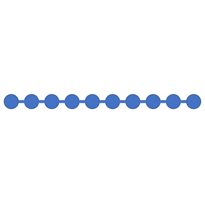
(a.1)n=10 path graph topology

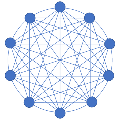
(b.1)n=10 complete graph topology

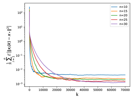
(a.2) The performance of path graph

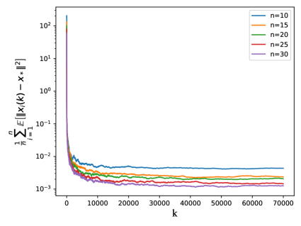
(b.2) The performance of complete graph

Figure 2: The performance of CDSA between path graph and complete graph topology. The results are averaged over 200 Monte Carlo sampling.

We demonstrate the empirical results in Fig. 2, where the empirical mean-squared error $\frac{1}{n}\sum\nolimits_{i=1}^{n}\mathbb{E}[||x_{i}(k)-x_{*}||^{2}]$ is calculated by averaging through 200 sample paths. We can see from the Subfigure (a.2) that for the path graph, when the iterate $k$ is small, the larger network size $n$ will lead to the higher mean-squared error $\frac{1}{n}\sum\nolimits_{i=1}^{n}\mathbb{E}[||x_{i}(k)-x_{*}||^{2}]$. However, with the increase of $k$, we observe a phase transition that a larger network size $n$ will lead to a smaller mean-squared error $\frac{1}{n}\sum\nolimits_{i=1}^{n}\mathbb{E}[||x_{i}(k)-x_{*}||^{2}]$ (namely faster convergence rate). This phenomenon matches the theoretical result (57): when $k$ is small, the main factor influencing the convergence rate is the second and third term concerning the network size $n$ via the distributed consensus protocol, while when $k$ is large, the first term inherited from centralized stochastic gradient descent dominates the convergence rate.

Compared it to the empirical performance of the complete graph shown in subfigure (b.2), we can find that from the beginning to the end, a larger network $n$ generates smaller errors, which also matches (58).

5.2 Logistic Regression

We further consider convex but not strongly convex problem, and use logistic regression to demonstrate that our algorithm can also leads to asymptotic convergence.

Consider the binary classification via logistic regression with unknown regularization parameter $\theta_{*}$,

$$\mathcal{C}_{\eta}(\theta_{*}):~{}\min_{\eta}\sum\nolimits_{i=1}^{n}\sum\nolimits_{j=1}^{m_{i}}\ln\left(1+e^{-\eta^{T}x_{ij}l_{ij}}\right)+\frac{\theta_{*}}{2}||\eta||^{2},$$

where $\theta_{*}$ can be obtained by a distributed parameter learning problem as follow,

$$\mathcal{L}_{\theta}:~{}\theta_{*}=\operatorname{argmin}\sum\nolimits_{i=1}^{n}\left(\theta-\alpha_{i}\right)^{2}.$$

As for agent $i$, its its own local computational problem and parameter learning problem are as follows.

$$f_{i}(\eta;\theta)=\min_{\eta}\sum\nolimits_{j=1}^{m_{i}}\ln\left(1+e^{-\eta^{T}x_{ij}l_{ij}}\right)+\frac{\theta_{*}}{2n}||\eta||^{2},~{}h_{i}(\theta)=\min_{\theta}(\theta-\alpha_{i})^{2}.$$

In this scenario, we set $\alpha_{i}=0.01\times i$ and let each agent $i\in\mathcal{N}$ possess dataset $\mathcal{D}_{i}\triangleq\{(x_{ij},l_{ij}):j=1,\cdots m_{i}\}$, where $x_{ij}$ represents a three-dimensional sample feature where the first dimension is $1$ and the other two dimension are selected from $N((1,0)^{T},\boldsymbol{I})$ or $N((0,1)^{T},\boldsymbol{I})$, while $l_{ij}$ is the related sample label $1$ or $-1$ respectively. Suppose that every agent holds a number of positive samples and negative samples which only accessible to itself.

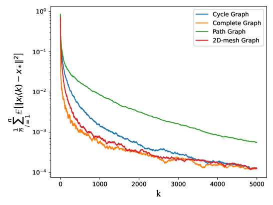
Figure 3: The performance of CDSA of $25$ agents under four topologies in table 2 for binary classification via logistic regression. The results are averaged over 200 Monte Carlo sampling.

We now compare the empirical performance of Algorithm 1 under four classes of graph topologies, path graph, cycle graph, 2D-mesh graph, and complete graph. We set $n=25$ and run Algorithm 1 with initial values $(\eta_{i}(0),\theta_{i}(0))=\boldsymbol{0}_{4}$ for all $i\in\mathcal{N}$, where the stepsize and weighted adjacency matrix are set the same as Ridge Regression. The empirical results are shown in fig. 3, which shows that the complete graph has best performance, 2D-mesh graph has the second-best performance, while the path graph displays the worst performance. These empirical findings match that listed in table 2, where the 2D-mesh graph has a larger spectral gap than the path graph and cycle path, hence leads to a lower mean-squared error.

6 Conclusions

In this work, we consider the distributed optimization problem $\min_{x}\frac{1}{n}\sum\nolimits_{i=1}^{n}f_{i}(x;\theta^{*})$ with the unknown parameter $\theta^{*}$ collaboratively solved by a distributed parameter learning problem $\min_{\theta}\frac{1}{n}\sum\nolimits_{i=1}^{n}h_{i}(\theta)$. Each agent only has access to its local computational problem $f_{i}(x,\theta)$ and its parameter learning problem $h_{i}(\theta)$. We propose a coupled distributed stochastic approximation algorithm for resolving this special distributed optimization, where agents can exchange information about decision variables $x$ and learning parameter $\theta$ with neighbors over a connected network. We quantitatively characterize the factors that influence the rate of convergence, and validates that the algorithm asymptotically achieves the optimal network-independent convergence rate compared to the centralized algorithm scheme. In addition, we analyze the transient time $K_{T}$, and show that when the iterate $k\geq K_{T}$, the dominate factor influencing the convergence rate is related to stochastic gradient descent, while for small $k<K_{T}$, the main factor influencing the convergence rate originates from the distributed average consensus method. Future work will consider more general problems under weakened assumptions. It is of interests to explore the accelerated algorithm to obtain a faster convergence rate.

Appendix A Proof of Lemma 3.1.1

Proof.

By using Assumption 2.2.2, we obtain that

$$\mathbb{E}[ ||\bar{g}(\boldsymbol{\mathbf{x}}(k),\boldsymbol{\mathbf{\theta}}(k),\boldsymbol{\mathbf{\xi}}(k))-\bar{\nabla}_{x}F(\boldsymbol{\mathbf{x}}(k),\boldsymbol{\mathbf{\theta}}(k))||^{2}|\mathcal{F}(k)]$$

$$=\mathbb{E}\left[\Big{\|}\frac{1}{n}\sum\nolimits_{i=1}^{n}g_{i}(x_{i}(k),\theta_{i}(k),\xi_{i}(k))-\frac{1}{n}\sum\nolimits_{i=1}^{n}\nabla_{x}f_{i}(x_{i}(k),\theta_{i}(k))\Big{\|}^{2}|\mathcal{F}(k)\right]$$

$$=\frac{1}{n^{2}}\sum\nolimits_{i=1}^{n}\mathbb{E}\left[||g_{i}(x_{i}(k),\theta_{i}(k),\xi_{i}(k))-\nabla_{x}f_{i}(x_{i}(k),\theta_{i}(k))||^{2}|\mathcal{F}(k)\right]$$

$$\leq\frac{1}{n^{2}}\sum\nolimits_{i=1}^{n}\left(\sigma_{x}^{2}+M_{x}||\nabla_{x}f_{i}(x_{i}(k),\theta_{i}(k))||^{2}\right)\leq\frac{\sigma_{x}^{2}}{n}+\frac{M_{x}\sum\nolimits_{i=1}^{n}||\nabla_{x}f_{i}(x_{i}(k),\theta_{i}(k))||^{2}}{n^{2}},$$ (59)

where the second equality use the fact that $\xi_{i},\forall i$ are independent random variables. By recalling assumption 2.2.1, we achieve

$$||\nabla_{x}f_{i}(x_{i}(k),\theta_{i}(k))||^{2}=||\nabla_{x}f_{i}(x_{i}(k),\theta_{i}(k))-\nabla_{x}f_{i}(x_{*},\theta_{i}(k))$$

$$\qquad+\nabla_{x}f_{i}(x_{*},\theta_{i}(k))-\nabla_{x}f_{i}(x_{*},\theta_{*})+\nabla_{x}f_{i}(x_{*},\theta_{*})||^{2}$$

$$\leq 3||\nabla_{x}f_{i}(x_{i}(k),\theta_{i}(k))-\nabla_{x}f_{i}(x_{*},\theta_{i}(k))||^{2}+3||\nabla_{x}f_{i}(x_{*},\theta_{i}(k))$$

$$\qquad-\nabla_{x}f_{i}(x_{*},\theta_{*})||^{2}+3||\nabla_{x}f_{i}(x_{*},\theta_{*})||^{2}$$

$$\leq 3L_{x}^{2}||x_{i}(k)-x_{*}||^{2}+3L_{\theta}^{2}||\theta_{i}(k)-\theta_{*}||^{2}+3||\nabla_{x}f_{i}(x_{*},\theta_{*})||^{2}.$$ (60)

Combining (60) and (59) yields the result (16).

Appendix B Proof of Lemma 3.1.2

Proof.

By recalling the definition of $\bar{x}(k),\bar{\theta}(k)$ and $\bar{\nabla}_{x}F(\boldsymbol{\mathbf{x}}(k),\boldsymbol{\mathbf{\theta}}(k))$ in (13) and (15), using Assumption 2.2.1, we have

$$||\nabla_{x}f(\bar{x}(k),\bar{\theta}(k))-\bar{\nabla}_{x}F(\boldsymbol{\mathbf{x}}(k),\boldsymbol{\mathbf{\theta}}(k))||$$

$$= ||\frac{1}{n}\sum\nolimits_{i=1}^{n}\nabla_{x}f_{i}(\bar{x}(k),\bar{\theta}(k))-\frac{1}{n}\sum\nolimits_{i=1}^{n}\nabla_{x}f_{i}(x_{i}(k),\theta_{i}(k))||$$

$$\leq \frac{1}{n}\sum\nolimits_{i=1}^{n}||\nabla_{x}f_{i}(\bar{x}(k),\bar{\theta}(k))-\nabla_{x}f_{i}(x_{i}(k),\theta_{i}(k))||$$

$$= \frac{1}{n}\sum\nolimits_{i=1}^{n}||\nabla_{x}f_{i}(\bar{x}(k),\bar{\theta}(k))-\nabla_{x}f_{i}(x_{i}(k),\bar{\theta}(k))+\nabla_{x}f_{i}(x_{i}(k),\bar{\theta}(k))-\nabla_{x}f_{i}(x_{i}(k),\theta_{i}(k))||$$

$$\leq \frac{1}{n}\sum_{i=1}^{n}\left[||\nabla_{x}f_{i}(\bar{x}(k),\bar{\theta}(k))-\nabla_{x}f_{i}(x_{i}(k),\bar{\theta}(k))||+||\nabla_{x}f_{i}(x_{i}(k),\bar{\theta}(k))-\nabla_{x}f_{i}(x_{i}(k),\theta_{i}(k))||\right]$$

$$\leq \frac{1}{n}\left(L_{x}\sum\nolimits_{i=1}^{n}||\bar{x}(k)-x_{i}(k)||+L_{\theta}\sum\nolimits_{i=1}^{n}||\bar{\theta}(k)-\theta_{i}(k)||\right)$$

$$\leq \frac{L_{x}}{\sqrt{n}}||\boldsymbol{\mathbf{x}}(k)-\boldsymbol{1}\bar{x}(k)^{T}||+\frac{L_{\theta}}{\sqrt{n}}||\boldsymbol{\mathbf{\theta}}(k)-\boldsymbol{1}\bar{\theta}(k)^{T}||,$$

where the last relation follows from Cauchy-Schwarz inequality.

Appendix C Proof of Lemma 3.2.1

Proof.

According to the definitions of $\bar{x}(k)$ and $\bar{g}(\boldsymbol{\mathbf{x}}(k),\boldsymbol{\mathbf{\theta}}(k),\boldsymbol{\mathbf{\xi}}(k))$ in (13) and (14), together with $\sum\nolimits_{i=1}^{n}w_{ij}=1$ form Assumption 2.2.3, we have

$$\bar{x}(k+1)=\frac{1}{n}\sum\nolimits_{i=1}^{n}\left(\sum\nolimits_{j=1}^{n}w_{ij}\left(x_{j}(k)-\alpha_{k}g_{j}(x_{j}(k),\theta_{j}(k),\xi_{j}(k))\right)\right)$$

$$=\frac{1}{n}\sum_{j=1}^{n}x_{j}(k)-\alpha_{k}\cdot\frac{1}{n}\sum_{j=1}^{n}g_{j}(x_{j}(k),\theta_{j}(k),\xi_{j}(k))=\bar{x}(k)-\alpha_{k}\bar{g}(\boldsymbol{\mathbf{x}}(k),\boldsymbol{\mathbf{\theta}}(k),\boldsymbol{\mathbf{\xi}}(k)).$$ (61)

Thus,

$$||\bar{x}(k+1)-x_{*}||^{2}=||\bar{x}(k)-\alpha_{k}\bar{g}(\boldsymbol{\mathbf{x}}(k),\boldsymbol{\mathbf{\theta}}(k),\boldsymbol{\mathbf{\xi}}(k))-x_{*}||^{2}$$

$$=||\bar{x}(k)-\alpha_{k}\bar{\nabla}_{x}F(\boldsymbol{\mathbf{x}}(k),\boldsymbol{\theta}(k))-x_{*}+\alpha_{k}\bar{\nabla}_{x}F(\boldsymbol{\mathbf{x}}(k),\boldsymbol{\theta}(k))-\alpha_{k}\bar{g}(\boldsymbol{\mathbf{x}}(k),\boldsymbol{\mathbf{\theta}}(k),\boldsymbol{\mathbf{\xi}}(k))||^{2}$$

$$=||\bar{x}(k)-\alpha_{k}\bar{\nabla}_{x}F(\boldsymbol{\mathbf{x}}(k),\boldsymbol{\theta}(k))-x_{*}||^{2}+\alpha_{k}^{2}||\bar{\nabla}_{x}F(\boldsymbol{\mathbf{x}}(k),\boldsymbol{\theta}(k))-\bar{g}(\boldsymbol{\mathbf{x}}(k),\boldsymbol{\mathbf{\theta}}(k),\boldsymbol{\mathbf{\xi}}(k))||^{2}$$

$$+2\alpha_{k}(\bar{x}(k)-\alpha_{k}\bar{\nabla}_{x}F(\boldsymbol{\mathbf{x}}(k),\boldsymbol{\theta}(k))-x_{*})^{T}\left(\bar{\nabla}_{x}F(\boldsymbol{\mathbf{x}}(k),\boldsymbol{\theta}(k))-\bar{g}\left(\boldsymbol{\mathbf{x}}(k),\boldsymbol{\mathbf{\theta}}(k),\boldsymbol{\mathbf{\xi}}(k)\right)\right).$$

In light of Assumption 2.2.2 and Lemma 3.1.1, by taking conditional expectation on both sides of above equation, we have

$$\mathbb{E}[|\bar{x}(k+1)-x_{*}||^{2} |\mathcal{F}(k)]|\leq||\bar{x}(k)-\alpha_{k}\bar{\nabla}_{x}F(\boldsymbol{\mathbf{x}}(k),\boldsymbol{\theta}(k))-x_{*}||^{2}$$

$$+\alpha_{k}^{2}\left(\frac{3M_{x}L_{x}^{2}}{n^{2}}||\boldsymbol{\mathbf{x}}(k)-\boldsymbol{1}x_{*}^{T}||^{2}+\frac{3M_{x}L_{\theta}^{2}}{n^{2}}||\boldsymbol{\mathbf{\theta}}(k)-\boldsymbol{1}\theta_{*}^{T}||^{2}+\frac{\bar{M}}{n}\right).$$ (62)

Next, we bound the first term on the right side of (62).

$$||\bar{x} (k)-\alpha_{k}\bar{\nabla}_{x}F(\boldsymbol{\mathbf{x}}(k),\boldsymbol{\theta}(k))-x_{*}||^{2}$$

$$=||\bar{x}(k)-\alpha_{k}\nabla_{x}f(\bar{x}(k);\bar{\theta}(k))-x_{*}+\alpha_{k}\nabla_{x}f(\bar{x}(k),\bar{\theta}(k))-\alpha_{k}\bar{\nabla}_{x}F(\boldsymbol{\mathbf{x}}(k),\boldsymbol{\theta}(k))||^{2}$$

$$=||\bar{x}(k)-\alpha_{k}\nabla_{x}f(\bar{x}(k),\bar{\theta}(k))-x_{*}||^{2}+\alpha_{k}^{2}||\nabla_{x}f(\bar{x}(k),\bar{\theta}(k))-\bar{\nabla}_{x}F(\boldsymbol{\mathbf{x}}(k),\boldsymbol{\theta}(k))||^{2}$$

$$+2\alpha_{k}(\bar{x}(k)-\alpha_{k}\nabla_{x}f(\bar{x}(k),\bar{\theta}(k))-x_{*})^{T}(\nabla_{x}f(\bar{x}(k),\bar{\theta}(k))-\bar{\nabla}_{x}F(\boldsymbol{\mathbf{x}}(k),\boldsymbol{\theta}(k)))$$

$$\leq\underbrace{||\bar{x}(k)-\alpha_{k}\nabla_{x}f(\bar{x}(k),\bar{\theta}(k))-x_{*}||^{2}}_{\text{Term 1}}+\underbrace{\alpha_{k}^{2}||\nabla_{x}f(\bar{x}(k),\bar{\theta}(k))-\bar{\nabla}_{x}F(\boldsymbol{\mathbf{x}}(k),\boldsymbol{\theta}(k))||^{2}}_{\text{Term 2}}$$

$$+\underbrace{2\alpha_{k}||\bar{x}(k)-\alpha_{k}\nabla_{x}f(\bar{x}(k),\bar{\theta}(k))-x_{*}||\times||\nabla_{x}f(\bar{x}(k),\bar{\theta}(k))-\bar{\nabla}_{x}F(\boldsymbol{\mathbf{x}}(k),\boldsymbol{\theta}(k))||}_{\text{Term 3}}.$$ (63)

As for Term 1, by leveraging the fact that $\alpha_{k}\leq\frac{1}{L}$, Lemma 2.2.1 indicates

$$||\bar{x}(k)-\alpha_{k}\nabla_{x}f(\bar{x}(k),\bar{\theta}(k))-x_{*}||^{2}\leq(1-\alpha_{k}\mu_{x})^{2}||\bar{x}(k)-x_{*}||^{2}.$$ (64)

By Lemma 3.1.2, Term 2 can be bounded as follow

$$\alpha_{k}^{2}||\nabla_{x}f(\bar{x}(k),\bar{\theta}(k))-\bar{\nabla}_{x}F(\boldsymbol{\mathbf{x}}(k),\boldsymbol{\theta}(k))||^{2}\leq\left(\frac{\alpha_{k}L_{x}||\boldsymbol{\mathbf{x}}(k)-\boldsymbol{1}\bar{x}(k)^{T}||}{\sqrt{n}}+\frac{\alpha_{k}L_{\theta}||\boldsymbol{\mathbf{\theta}}(k)-\boldsymbol{1}\bar{\theta}(k)^{T}||}{\sqrt{n}}\right)^{2}$$

$$\leq\frac{\alpha_{k}^{2}L_{x}^{2}||\boldsymbol{\mathbf{x}}(k)-\boldsymbol{1}\bar{x}(k)^{T}||^{2}}{n}+\frac{\alpha_{k}^{2}L_{\theta}^{2}||\boldsymbol{\mathbf{\theta}}(k)-\boldsymbol{1}\bar{\theta}(k)^{T}||^{2}}{n}+\frac{2L_{x}L_{\theta}\alpha_{k}^{2}}{n}||\boldsymbol{\mathbf{x}}(k)-\boldsymbol{1}\bar{x}(k)^{T}||\times||\boldsymbol{\mathbf{\theta}}(k)-\boldsymbol{1}\bar{\theta}(k)^{T}||.$$ (65)

Finally, Term 3 can be bounded by invoking the same transformation approches used in Term 1 and Term 2:

$$\text{Term 3}\leq 2\alpha_{k}(1-\alpha_{k}\mu_{x})||\bar{x}(k)-x_{*}||\left(\frac{L_{x}}{\sqrt{n}}||\boldsymbol{\mathbf{x}}(k)-\boldsymbol{1}\bar{x}(k)^{T}||\frac{L_{\theta}}{\sqrt{n}}||\boldsymbol{\mathbf{\theta}}(k)-\boldsymbol{1}\bar{\theta}(k)^{T}||\right)$$

$$\leq\frac{2\alpha_{k}L_{x}(1-\alpha_{k}\mu_{x})||\bar{x}(k)-x_{*}||||\boldsymbol{\mathbf{x}}(k)-\boldsymbol{1}\bar{x}(k)^{T}||}{\sqrt{n}}+\frac{2\alpha_{k}L_{\theta}(1-\alpha_{k}\mu_{x})||\bar{x}(k)-x_{*}||||\boldsymbol{\mathbf{\theta}}(k)-\boldsymbol{1}\bar{\theta}(k)^{T}||}{\sqrt{n}}.$$ (66)

In light of relation (63)$\sim$(66), taking full expectation on both side of relation (62) yields the result (A). Furthermore by using mean value inequality $2ab\leq a^{2}+b^{2}$, we rearrange (21) and obtain that

$$U_{1}(k+1) \leq(1-\alpha_{k}\mu_{x})^{2}U_{1}(k)+\frac{\alpha_{k}^{2}L_{x}^{2}}{n}V_{1}(k)+\frac{\alpha_{k}^{2}L_{\theta}^{2}}{n}V_{2}(k)+\frac{\alpha_{k}^{2}L_{x}^{2}}{n}V_{1}(k)+\frac{\alpha_{k}^{2}L_{\theta}^{2}}{n}V_{2}(k)$$

$$+(1-\alpha_{k}\mu_{x})^{2}c_{1}U_{1}(k)+\frac{\alpha_{k}^{2}L_{x}^{2}}{n}\cdot\frac{1}{c_{1}}V_{1}(k)+(1-\alpha_{k}\mu_{x})^{2}c_{2}U_{1}(k)+\frac{\alpha_{k}^{2}L_{\theta}^{2}}{n}\cdot\frac{1}{c_{2}}V_{2}(k)$$

$$\qquad+\alpha_{k}^{2}\left(\frac{3M_{x}L_{x}^{2}}{n^{2}}\mathbb{E}[||\boldsymbol{\mathbf{x}}(k)-\boldsymbol{1}x_{*}^{T}||]+\frac{3M_{x}L_{\theta}^{2}}{n^{2}}\mathbb{E}[||\boldsymbol{\theta}(k)-\boldsymbol{1}\theta_{*}^{T}||]+\frac{\bar{M}}{n}\right)$$

$$\leq(1+c_{1}+c_{2})(1-\alpha_{k}\mu_{x})^{2}U_{1}(k)+(2+\frac{1}{c_{1}})\frac{\alpha_{k}^{2}L_{x}^{2}}{n}V_{1}(k)+(2+\frac{1}{c_{2}})\frac{\alpha_{k}^{2}L_{\theta}^{2}}{n}V_{2}(k)$$

$$\quad+\alpha_{k}^{2}\left(\frac{3M_{x}L_{x}^{2}}{n^{2}}\mathbb{E}[||\boldsymbol{\mathbf{x}}(k)-\boldsymbol{1}x_{*}^{T}||]+\frac{3M_{x}L_{\theta}^{2}}{n^{2}}\mathbb{E}[||\boldsymbol{\theta}(k)-\boldsymbol{1}\theta_{*}^{T}||]+\frac{\bar{M}}{n}\right),$$ (67)

where $c_{1},c_{2}>0$. Take $c_{1}=c_{2}=\frac{3}{16}\alpha_{k}\mu_{x}$, then $c_{1}+c_{2}=\frac{3}{8}\alpha_{k}\mu_{x}$. Noticing that $\alpha_{k}\leq\frac{1}{3\mu_{x}}$, i.e. $\alpha_{k}\mu_{x}\leq\frac{1}{3}$, we have

$$(1+c_{1}+c_{2})(1-\alpha_{k}\mu_{x})^{2}=1-\frac{13}{8}\alpha_{k}\mu_{x}+\frac{1}{4}\alpha_{k}^{2}\mu_{x}^{2}+\frac{3}{8}\alpha_{k}^{3}\mu_{x}^{3}$$ (68)

$$\leq 1-\frac{13}{8}\alpha_{k}\mu_{x}+\frac{1}{12}\alpha_{k}\mu_{x}+\frac{3}{8}\times\frac{1}{9}\alpha_{k}\mu_{x}=1-\frac{3}{2}\alpha_{k}\mu_{x},$$

and $(2+\frac{1}{c_{m}})\alpha_{k}\leq\frac{6}{\mu_{x}},m=1,2$. Plug them into (67) yeilds the result B.

Appendix D Proof of Lemma 3.2.2

Proof.

Recalling the definition of $\mathbf{g}(\boldsymbol{\mathbf{x}},\boldsymbol{\theta},\boldsymbol{\mathbf{\xi}})$ in (8) and relation $\bar{x}(k+1)=\bar{x}(k)-\alpha_{k}\bar{g}(\boldsymbol{\mathbf{x}}(k),\boldsymbol{\mathbf{\theta}}(k),\boldsymbol{\mathbf{\xi}}(k))$ in eq. 61, and using (10), we have

$$\boldsymbol{\mathbf{x}}(k+1)-\boldsymbol{1} \bar{x}(k+1)=W\left(\boldsymbol{\mathbf{x}}(k)-\alpha_{k}\mathbf{g}\left(\boldsymbol{\mathbf{x}}(k),\boldsymbol{\mathbf{\theta}}(k),\boldsymbol{\xi}(k)\right)\right)-\boldsymbol{1}(\bar{x}(k)-\alpha_{k}\bar{g}\left(\boldsymbol{\mathbf{x}}(k),\boldsymbol{\mathbf{\theta}}(k),\boldsymbol{\mathbf{\xi}}(k)\right))$$

$$=(W-\frac{\boldsymbol{1}\boldsymbol{1}^{T}}{n})\left[(\boldsymbol{\mathbf{x}}(k)-\boldsymbol{1}\bar{x}(k))-\alpha_{k}(\mathbf{g}\left(\boldsymbol{\mathbf{x}}(k),\boldsymbol{\mathbf{\theta}}(k),\boldsymbol{\xi}(k)\right)-\boldsymbol{1}\bar{g}\left(\boldsymbol{\mathbf{x}}(k),\boldsymbol{\mathbf{\theta}}(k),\boldsymbol{\mathbf{\xi}}(k)\right))\right].$$ (69)

Thus by Lemma 2.2.2, we obtain

$$||\boldsymbol{\mathbf{x}} (k+1)-\boldsymbol{1}\bar{x}(k+1)||^{2}$$

$$\leq\rho_{w}^{2}||(\boldsymbol{\mathbf{x}}(k)-\boldsymbol{1}\bar{x}(k))-\alpha_{k}(\mathbf{g}\left(\boldsymbol{\mathbf{x}}(k),\boldsymbol{\mathbf{\theta}}(k),\boldsymbol{\xi}(k)\right)-\boldsymbol{1}\bar{g}\left(\boldsymbol{\mathbf{x}}(k),\boldsymbol{\mathbf{\theta}}(k),\boldsymbol{\mathbf{\xi}}(k)\right)||^{2}$$

$$=\rho_{w}^{2}\big{[}||\boldsymbol{\mathbf{x}}(k)-\boldsymbol{1}\bar{x}(k)||^{2}+\underbrace{\alpha_{k}^{2}||\mathbf{g}\left(\boldsymbol{\mathbf{x}}(k),\boldsymbol{\mathbf{\theta}}(k),\boldsymbol{\xi}(k)\right)-\boldsymbol{1}\bar{g}\left(\boldsymbol{\mathbf{x}}(k),\boldsymbol{\mathbf{\theta}}(k),\boldsymbol{\mathbf{\xi}}(k)\right)||^{2}}_{\text{Term 4}}$$

$$\quad\underbrace{-2\alpha_{k}(\boldsymbol{\mathbf{x}}(k)-\boldsymbol{1}\bar{x}(k))^{T}(\mathbf{g}\left(\boldsymbol{\mathbf{x}}(k),\boldsymbol{\mathbf{\theta}}(k),\boldsymbol{\xi}(k)\right)-\boldsymbol{1}\bar{g}\left(\boldsymbol{\mathbf{x}}(k),\boldsymbol{\mathbf{\theta}}(k),\boldsymbol{\mathbf{\xi}}(k)\right)}_{\text{Term 5}}\big{]}$$ (70)

In the following, we will separately consider Term 4 and Term 5. Note that

$$\|I-\boldsymbol{1}\boldsymbol{1}^{T}/n\|\leq 1.$$ (71)

The by using Assumptions 2.2.2 (a) and 2.2.2 (b), we derive

$$\mathbb{E}\left[\alpha_{k}^{2}\right. \left.||\mathbf{g}(\boldsymbol{\mathbf{x}}(k),\boldsymbol{\mathbf{\theta}}(k),\boldsymbol{\xi}(k))-\boldsymbol{1}\bar{g}\left(\boldsymbol{\mathbf{x}}(k),\boldsymbol{\mathbf{\theta}}(k),\boldsymbol{\mathbf{\xi}}(k)\right)||^{2}|\mathcal{F}(k)\right]$$

$$=\alpha_{k}^{2}\mathbb{E}\left[||\nabla_{x}\boldsymbol{F}(\boldsymbol{\mathbf{x}}(k),\boldsymbol{\theta}(k))-\boldsymbol{1}\bar{\nabla}_{x}F(\boldsymbol{\mathbf{x}}(k),\boldsymbol{\theta}(k))-\nabla_{x}\boldsymbol{F}(\boldsymbol{\mathbf{x}}(k),\boldsymbol{\theta}(k))\right.$$

$$\left.+\boldsymbol{1}\bar{\nabla}_{x}F(\boldsymbol{\mathbf{x}}(k),\boldsymbol{\theta}(k))+\mathbf{g}(\boldsymbol{\mathbf{x}}(k),\boldsymbol{\mathbf{\theta}}(k)),\boldsymbol{\xi}(k)-\boldsymbol{1}\bar{g}\left(\boldsymbol{\mathbf{x}}(k),\boldsymbol{\mathbf{\theta}}(k),\boldsymbol{\mathbf{\xi}}(k)\right)||^{2}|\mathcal{F}(k)\right]$$

$$=\alpha_{k}^{2}||\nabla_{x}\boldsymbol{F}(\boldsymbol{\mathbf{x}}(k),\boldsymbol{\theta}(k))-\boldsymbol{1}\bar{\nabla}_{x}F(\boldsymbol{\mathbf{x}}(k),\boldsymbol{\theta}(k))||^{2}+\alpha_{k}^{2}\mathbb{E}[||\nabla_{x}\boldsymbol{F}(\boldsymbol{\mathbf{x}}(k),\boldsymbol{\theta}(k))$$

$$\qquad-\mathbf{g}((\boldsymbol{\mathbf{x}}(k),\boldsymbol{\mathbf{\theta}}(k),\boldsymbol{\xi}(k))-\boldsymbol{1}(\bar{\nabla}_{x}F(\boldsymbol{\mathbf{x}}(k),\boldsymbol{\theta}(k))-\bar{g}(\boldsymbol{\mathbf{x}}(k),\boldsymbol{\mathbf{\theta}}(k)))||^{2}|\mathcal{F}(k)]$$

$$\overset{\eqref{1_leq1}}{\leq}\alpha_{k}^{2}\left[||\nabla_{x}\boldsymbol{F}(\boldsymbol{\mathbf{x}}(k),\boldsymbol{\theta}(k))-\boldsymbol{1}\bar{\nabla}_{x}F(\boldsymbol{\mathbf{x}}(k),\boldsymbol{\theta}(k))||^{2}\right.$$

$$\left.\qquad+\mathbb{E}[||\nabla_{x}\boldsymbol{F}(\boldsymbol{\mathbf{x}}(k),\boldsymbol{\theta}(k))-\mathbf{g}(\boldsymbol{\mathbf{x}}(k),\boldsymbol{\mathbf{\theta}}(k),\boldsymbol{\xi}(k))||^{2}|\mathcal{F}(k)]\right]$$

$$\leq\alpha_{k}^{2}||\nabla_{x}\boldsymbol{F}(\boldsymbol{\mathbf{x}}(k),\boldsymbol{\theta}(k))-\boldsymbol{1}\bar{\nabla}_{x}F(\boldsymbol{\mathbf{x}}(k),\boldsymbol{\theta}(k))||^{2}+\alpha_{k}^{2}n\sigma_{x}^{2}+\alpha_{k}^{2}M_{x}||\nabla_{x}\boldsymbol{F}(\boldsymbol{\mathbf{x}}(k),\boldsymbol{\theta}(k))||^{2}.$$ (72)

Recalling Assumption 2.2.2 (a), we obtain that

$$\mathbb{E}\big{[} -2\alpha_{k}(\boldsymbol{\mathbf{x}}(k)-\boldsymbol{1}\bar{x}(k))^{T}\left(\mathbf{g}(\boldsymbol{\mathbf{x}}(k),\boldsymbol{\mathbf{\theta}}(k),\boldsymbol{\xi}(k))-\boldsymbol{1}\bar{g}\left(\boldsymbol{\mathbf{x}}(k),\boldsymbol{\mathbf{\theta}}(k),\boldsymbol{\mathbf{\xi}}(k)\right)\right)|\mathcal{F}(k)\big{]}$$

$$=-2\alpha_{k}(\boldsymbol{\mathbf{x}}(k)-\boldsymbol{1}\bar{x}(k))^{T}\left(\nabla_{x}\boldsymbol{F}(\boldsymbol{\mathbf{x}}(k),\boldsymbol{\theta}(k))-\boldsymbol{1}\bar{\nabla}_{x}F(\boldsymbol{\mathbf{x}}(k),\boldsymbol{\theta}(k))\right),$$ (73)

In light of (70),(72) and (73), we have

$$\frac{1}{\rho_{w}^{2}}\mathbb{E}[ ||\boldsymbol{\mathbf{x}}(k+1)-\boldsymbol{1}\bar{x}(k+1)||^{2}|\mathcal{F}(k)]$$

$$\leq||\boldsymbol{\mathbf{x}}(k)-\boldsymbol{1}\bar{x}(k)||^{2}+\alpha_{k}^{2}||\nabla_{x}\boldsymbol{F}(\boldsymbol{\mathbf{x}}(k),\boldsymbol{\theta}(k))-\boldsymbol{1}\bar{\nabla}_{x}F(\boldsymbol{\mathbf{x}}(k),\boldsymbol{\theta}(k))||^{2}$$

$$\quad+\alpha_{k}^{2}n\sigma_{x}^{2}+\alpha_{k}^{2}M_{x}||\nabla_{x}\boldsymbol{F}(\boldsymbol{\mathbf{x}}(k),\boldsymbol{\theta}(k))||^{2}$$

$$\quad-2\alpha_{k}(\boldsymbol{\mathbf{x}}(k)-\boldsymbol{1}\bar{x}(k))^{T}(\nabla_{x}\boldsymbol{F}(\boldsymbol{\mathbf{x}}(k),\boldsymbol{\theta}(k))-\boldsymbol{1}\bar{\nabla}_{x}F(\boldsymbol{\mathbf{x}}(k),\boldsymbol{\theta}(k)))$$

$$\leq||\boldsymbol{\mathbf{x}}(k)-\boldsymbol{1}\bar{x}(k)||^{2}+\alpha_{k}^{2}||\nabla_{x}\boldsymbol{F}(\boldsymbol{\mathbf{x}}(k),\boldsymbol{\theta}(k))-\boldsymbol{1}\bar{\nabla}_{x}F(\boldsymbol{\mathbf{x}}(k),\boldsymbol{\theta}(k))||^{2}$$

$$\quad+\alpha_{k}^{2}n\sigma_{x}^{2}+\alpha_{k}^{2}M_{x}||\nabla_{x}\boldsymbol{F}(\boldsymbol{\mathbf{x}}(k),\boldsymbol{\theta}(k))||^{2}$$

$$\quad+c_{3}||\boldsymbol{\mathbf{x}}(k)-\boldsymbol{1}\bar{x}(k)||^{2}+\frac{1}{c_{3}}\alpha_{k}^{2}||\nabla_{x}\boldsymbol{F}(\boldsymbol{\mathbf{x}}(k),\boldsymbol{\theta}(k))-\boldsymbol{1}\bar{\nabla}_{x}F(\boldsymbol{\mathbf{x}}(k),\boldsymbol{\theta}(k))||^{2}$$

$$\leq(1+c_{3})||\boldsymbol{\mathbf{x}}(k)-\boldsymbol{1}\bar{x}(k)||^{2}+\alpha_{k}^{2}n\sigma_{x}^{2}+\alpha_{k}^{2}\left(1+M_{x}+\frac{1}{c_{3}}\right)||\nabla_{x}\boldsymbol{F}(\boldsymbol{\mathbf{x}}(k),\boldsymbol{\theta}(k))||^{2},$$ (74)

where $c_{3}>0$ is arbitrary, and the last inequality also uses the porperty in (71).

We then consider the upper bound of $||\nabla_{x}F(\boldsymbol{\mathbf{x}}(k),\boldsymbol{\theta}(k))||^{2}$ as follow,

$$||\nabla_{x}\boldsymbol{F}(\boldsymbol{\mathbf{x}}(k),\boldsymbol{\theta}(k))||^{2}=||\nabla_{x}\boldsymbol{F}(\boldsymbol{\mathbf{x}}(k),\boldsymbol{\theta}(k))-\nabla_{x}\boldsymbol{F}(\boldsymbol{1}x_{*}^{T},\boldsymbol{\theta}(k))$$

$$\qquad\qquad+\nabla_{x}\boldsymbol{F}(\boldsymbol{1}x_{*}^{T},\boldsymbol{\theta}(k))-\nabla_{x}\boldsymbol{F}(\boldsymbol{1}x_{*}^{T},\boldsymbol{1}\theta_{*}^{T})+\nabla_{x}\boldsymbol{F}(\boldsymbol{1}x_{*}^{T},\boldsymbol{1}\theta_{*}^{T})||^{2}$$

$$\leq 3||\nabla_{x}\boldsymbol{F}(\boldsymbol{\mathbf{x}}(k),\boldsymbol{\theta}(k))-\nabla_{x}\boldsymbol{F}(\boldsymbol{1}x_{*}^{T},\boldsymbol{\theta}(k))||^{2}$$

$$\quad+3||\nabla_{x}\boldsymbol{F}(\boldsymbol{1}x_{*}^{T},\boldsymbol{\theta}(k))-\nabla_{x}\boldsymbol{F}(\boldsymbol{1}x_{*}^{T},\boldsymbol{1}\theta_{*}^{T})||^{2}+3||\nabla_{x}\boldsymbol{F}(\boldsymbol{1}x_{*}^{T},\boldsymbol{1}\theta_{*}^{T})||^{2}$$

$$\leq 3L_{x}^{2}||\boldsymbol{\mathbf{x}}(k)-\boldsymbol{1}\bar{x}(k)||^{2}+3L_{\theta}^{2}||\boldsymbol{\theta}(k)-\boldsymbol{1}\theta_{*}^{T}||^{2}+3||\nabla_{x}\boldsymbol{F}(\boldsymbol{1}x_{*}^{T},\boldsymbol{1}\theta_{*}^{T})||^{2}.$$ (75)

Let $c_{3}=\frac{1-\rho_{w}^{2}}{2}$. Combining (74) and (75), we obtain that

$$\frac{1}{\rho_{w}^{2}}\mathbb{E}[||\boldsymbol{\mathbf{x}} (k+1)-\boldsymbol{1}\bar{x}(k+1)||^{2}|\mathcal{F}(k)]$$

$$\leq\frac{3-\rho_{w}^{2}}{2}||\boldsymbol{\mathbf{x}}(k)-\boldsymbol{1}\bar{x}(k)||^{2}+3\alpha_{k}^{2}\left(\frac{3}{1-\rho_{w}^{2}}+M_{x}\right)\left(L_{x}^{2}||\boldsymbol{\mathbf{x}}(k)-\boldsymbol{1}\bar{x}(k)||^{2}\right.$$

$$\qquad\left.+L_{\theta}^{2}||\boldsymbol{\theta}(k)-\boldsymbol{1}\theta_{*}^{T}||^{2}+||\nabla_{x}\boldsymbol{F}(\boldsymbol{1}x_{*}^{T},\boldsymbol{1}\theta_{*}^{T})||^{2}\right)+\alpha_{k}^{2}n\sigma_{x}^{2}.$$ (76)

Note that $\rho_{w}^{2}(\frac{3-\rho_{w}^{2}}{2})\leq\frac{3+\rho_{w}^{2}}{4}$ by $\rho_{w}\in(0,1)$. Then by taking full expectation on both sides of (76) and multiplying $\rho_{w}^{2}$ leads to the result (24).

Appendix E Proof of Lemma 3.3.1

Proof.

For any $k\geq 0$, in order to bound $\mathbb{E}[||\boldsymbol{\mathbf{x}}(k)-\boldsymbol{1}x_{*}^{T}||^{2}]$, we firstly consider bounding $\mathbb{E}[||x_{i}(k)-\alpha_{k}g_{i}(x_{i}(k),\theta_{i}(k),\xi_{i}(k))-x_{*}||^{2}]$ for all $i\in\mathcal{N}$. By using Assumption 2.2.1 (i) and Assumption 2.2.2 (c), we have

$$\mathbb{E}[||x_{i}(k)-\alpha_{k}g_{i}(x_{i}(k),\theta_{i}(k),\xi_{i}(k))-x_{*}||^{2}|\mathcal{F}(k)]=||x_{i}(k)-x_{*}-\alpha_{k}\nabla_{x}f_{i}(x_{i}(k),\theta_{i}(k))||^{2}$$

$$\qquad+\alpha_{k}^{2}\mathbb{E}\left[||\nabla_{x}f_{i}(x_{i}(k),\theta_{i}(k))-g_{i}(x_{i}(k),\theta_{i}(k),\xi_{i}(k))||^{2}|\mathcal{F}(k)\right]$$

$$\leq||x_{i}(k)-x_{*}||^{2}-2\alpha_{k}\nabla_{x}f_{i}(x_{i}(k),\theta_{i}(k))^{T}(x_{i}(k)-x_{*})$$

$$\qquad+\alpha_{k}^{2}||\nabla_{x}f_{i}(x_{i}(k),\theta_{i}(k))||^{2}+\alpha_{k}^{2}(\sigma_{x}^{2}+M_{x}||\nabla_{x}f_{i}(x_{i}(k),\theta_{i}(k))||^{2})$$

$$\leq||x_{i}(k)-x_{*}||^{2}-2\alpha_{k}\mu_{x}||x_{i}(k)-x_{*}||^{2}+2\alpha_{k}||\nabla_{x}f_{i}(x_{*},\theta_{i}(k))||||x_{i}(k)-x_{*}||$$

$$\qquad+\alpha_{k}^{2}(1+M_{x})||\nabla_{x}f_{i}(x_{i}(k),\theta_{i}(k))||^{2}+\alpha_{k}^{2}\sigma_{x}^{2},$$ (77)

Consider the upper bound of the term $||\nabla_{x}f_{i}(x_{i}(k),\theta_{i}(k))||^{2}$ on the right side of above inequality. Using Assumption 2.2.1 (i) and (ii), we have

$$||\nabla_{x}f_{i}(x_{i}(k),\theta_{i}(k))||^{2} =||\nabla_{x}f_{i}(x_{i}(k),\theta_{i}(k))-\nabla_{x}f_{i}(x_{*},\theta_{i}(k))+\nabla_{x}f_{i}(x_{*},\theta_{i}(k))$$

$$\qquad-\nabla_{x}f_{i}(x_{*},\theta_{*})+\nabla_{x}f_{i}(x_{*},\theta_{*})||$$

$$\leq 3L_{x}^{2}||x_{i}(k)-x_{*}||^{2}+3L_{\theta}^{2}||\theta_{i}(k)-\theta_{*}||^{2}+3||\nabla_{x}f_{i}(x_{*},\theta_{*})||^{2}.$$ (78)

We can similarly obtain $||\nabla_{x}f_{i}(x_{*},\theta_{i}(k))||^{2}\leq 2L_{\theta}^{2}||\theta_{i}(k)-\theta_{*}||^{2}+2||\nabla_{x}f_{i}(x_{*},\theta_{*})||^{2}$. Combining (78) and (77), it produces

$$\mathbb{E}[||x_{i}(k) -\alpha_{k}g_{i}(x_{i}(k),\theta_{i}(k),\xi_{i}(k))-x_{*}||^{2}|\mathcal{F}(k)]\leq||x_{i}(k)-x_{*}||^{2}-2\alpha_{k}\mu_{x}||x_{i}(k)-x_{*}||^{2}$$

$$\quad+\alpha_{k}^{2}\sigma_{x}^{2}+2\alpha_{k}\sqrt{2L_{\theta}^{2}||\theta_{i}(k)-\theta_{*}||^{2}+2||\nabla_{x}f_{i}(x_{*},\theta_{*})||^{2}}||x_{i}(k)-x_{*}||$$

$$\quad+\alpha_{k}^{2}(1+M_{x})(3L_{x}^{2}||x_{i}(k)-x_{*}||^{2}+3L_{\theta}^{2}||\theta_{i}(k)-\theta_{*}||^{2}+3||\nabla_{x}f_{i}(x_{*},\theta_{*})||^{2})$$

$$\leq(1-2\alpha_{k}\mu_{x}+3\alpha_{k}^{2}(1+M_{x})L_{x}^{2})||x_{i}(k)-x_{*}||^{2}$$

$$\quad+2\alpha_{k}\sqrt{2L_{\theta}^{2}||\theta_{i}(k)-\theta_{*}||^{2}+2||\nabla_{x}f_{i}(x_{*},\theta_{*})||^{2}}||x_{i}(k)-x_{*}||$$

$$\quad+\alpha_{k}^{2}[3(1+M_{x})L_{\theta}^{2}||\theta_{i}(k)-\theta_{*}||^{2}+3(1+M_{x})||\nabla_{x}f_{i}(x_{*},\theta_{*})||^{2}+\sigma_{x}^{2}].$$ (79)

From the definition of $K$ in (26), for all $k\geq 0$, we have $\alpha_{k}\leq\frac{\mu_{x}}{3(1+M_{x})L_{x}^{2}}$. Recall the fact that $\mathbb{E}[||\theta_{i}(k)-\theta_{*}||^{2}]\leq\hat{\Theta}_{i}$ in (27). By taking full expectation on both sides of (79) and using $\mathbb{E}[||x_{i}(k)-x_{*}||]\leq\sqrt{\mathbb{E}[||x_{i}(k)-x_{*}||^{2}]}$, we have

$$\mathbb{E}[||x_{i}(k)- \alpha_{k}g_{i}(x_{i}(k),\theta_{i}(k),\xi_{i}(k))-x_{*}||^{2}]\leq(1-\alpha_{k}\mu_{x})\mathbb{E}[||x_{i}(k)-x_{*}||^{2}]$$

$$\qquad+2\alpha_{k}\sqrt{2L_{\theta}^{2}\hat{\Theta}_{i}+2||\nabla_{x}f_{i}(x_{*},\theta_{*})||^{2}}\sqrt{\mathbb{E}[||x_{i}(k)-x_{*}||^{2}]}$$

$$\qquad+\alpha_{k}\left[\frac{\mu_{x}L_{\theta}^{2}}{L_{x}^{2}}\hat{\Theta}_{i}+\frac{\mu_{x}}{L_{x}^{2}}||\nabla_{x}f_{i}(x_{*},\theta_{*})||^{2}+\frac{\mu_{x}\sigma_{x}^{2}}{3(1+M_{x})L_{x}^{2}}\right]$$

$$\quad\leq\mathbb{E}[||x_{i}(k)-x_{*}||^{2}]-\alpha_{k}\bigg{[}\mu_{x}\mathbb{E}||x_{i}(k)-x_{*}||^{2}$$

$$\qquad-2\sqrt{2L_{\theta}^{2}\hat{\Theta}_{i}+2||\nabla_{x}f_{i}(x_{*},\theta_{*})||^{2}}\sqrt{\mathbb{E}[||x_{i}(k)-x_{*}||^{2}]}$$

$$\qquad-\left(\frac{\mu_{x}L_{\theta}^{2}}{L_{x}^{2}}\hat{\Theta}_{i}+\frac{\mu_{x}}{L_{x}^{2}}||\nabla_{x}f_{i}(x_{*},\theta_{*})||^{2}+\frac{\mu_{x}\sigma_{x}^{2}}{3(1+M_{x})L_{x}^{2}}\right)\bigg{]}.$$ (80)

Next, we consider the following set:

$$\mathcal{X}_{i}\triangleq\bigg{\{}q\geq 0: \mu_{x}q-2\sqrt{2L_{\theta}^{2}\hat{\Theta}_{i}+2||\nabla_{x}f_{i}(x_{*},\theta_{*})||^{2}}\sqrt{q}$$

$$-\frac{\mu_{x}}{3L_{x}^{2}}\left(3L_{\theta}^{2}\hat{\Theta}_{i}+3||\nabla_{x}f_{i}(x_{*},\theta_{*})||^{2}+\frac{\sigma_{x}^{2}}{1+M_{x}}\right)\leq 0\bigg{\}}.$$ (81)

It can be seen that $\mathcal{X}_{i}$ is non-empty and compact. If $\mathbb{E}[||x_{i}(k)-x_{*}||^{2}]\notin\mathcal{X}_{i}$, in light of (80) we known that $\mathbb{E}[||x_{i}(k)-\alpha_{k}g_{i}(x_{i}(k),\theta_{i}(k),\xi_{i}(k))-x_{*}||^{2}]\leq\mathbb{E}[||x_{i}(k)-x_{*}||^{2}]$. While for $\mathbb{E}[||x_{i}(k)-x_{*}||^{2}]\in\mathcal{X}_{i}$, by using $\alpha_{k}\leq\frac{\mu_{x}}{3(1+M_{x})L_{x}^{2}}$, we derive

$$\mathbb{E}[||x_{i}(k)-\alpha_{k}g_{i}(x_{i}(k),\theta_{i}(k),\xi_{i}(k))-x_{*}||^{2}]$$

$$\leq\max_{q\in\mathcal{X}_{i}}\Bigg{\{}q-\frac{\mu_{x}}{3(1+M_{x})L_{x}^{2}}\Big{[}\mu_{x}q-2\sqrt{2L_{\theta}^{2}\hat{\Theta}_{i}+2||\nabla_{x}f_{i}(x_{*},\theta_{*})||^{2}}\sqrt{q}$$

$$\qquad-\frac{\mu_{x}}{3L_{x}^{2}}\left(3L_{\theta}^{2}\hat{\Theta}_{i}+3||\nabla_{x}f_{i}(x_{*},\theta_{*})||^{2}+\frac{\sigma_{x}^{2}}{1+M_{x}}\right)\Big{]}\Bigg{\}}\triangleq R_{i}.$$ (82)

Based on previous arguments, we conclude that for all $k>0$,

$$\mathbb{E}[||x_{i}(k)-\alpha_{k}g_{i}(x_{i}(k),\theta_{i}(k),\xi_{i}(k))-x_{*}||^{2}]\leq\max\left\{\mathbb{E}[||x_{i}(k)-x_{*}||^{2}],R_{i}\right\}.$$ (83)

In light of $W\boldsymbol{1}=\boldsymbol{1}$, by noting from (10) that

$$\|\boldsymbol{\mathbf{x}}(k+1)-\boldsymbol{1}x_{*}^{T}\|^{2} \leq\|W\|^{2}\|\boldsymbol{\mathbf{x}}(k)-\alpha_{k}\mathbf{g}(\boldsymbol{\mathbf{x}}(k),\boldsymbol{\theta}(k),\boldsymbol{\mathbf{\xi}}(k))-\boldsymbol{1}x_{*}^{T}\|^{2}$$

$$\leq\|\boldsymbol{\mathbf{x}}(k)-\alpha_{k}\mathbf{g}(\boldsymbol{\mathbf{x}}(k),\boldsymbol{\theta}(k),\boldsymbol{\mathbf{\xi}}(k))-\boldsymbol{1}x_{*}^{T}\|^{2}.$$ (84)

This together with (83) produces

$$\mathbb{E}[||\boldsymbol{\mathbf{x}}(k)-\boldsymbol{1}x_{*}^{T}||^{2}]\leq\max\left\{\mathbb{E}[||\boldsymbol{\mathbf{x}}(0)-\boldsymbol{1}x_{*}^{T}||^{2}],\sum\nolimits_{i=1}^{n}R_{i}\right\}$$ (85)

In the following, we will give an upper bound of $R_{i}$. From the definition of $\mathcal{X}_{i}$ in (81), we know that the right zero of the upward opening parabola is

$$\sqrt{q_{i}}=\frac{1}{2\mu_{x}}\Bigg{[}2\sqrt{2L_{\theta}^{2}\hat{\Theta}_{i}+2||\nabla_{x}f_{i}(x_{*},\theta_{*})||^{2}}$$

$$+\sqrt{4(2L_{\theta}^{2}\hat{\Theta}_{i}+2||\nabla_{x}f_{i}(x_{*},\theta_{*})||^{2})+\frac{4\mu_{x}^{2}}{3L_{x}^{2}}\left(3L_{\theta}^{2}\hat{\Theta}_{i}+3||\nabla_{x}f_{i}(x_{*},\theta_{*})||^{2}+\frac{\sigma_{x}^{2}}{1+M_{x}}\right)}\Bigg{]}.$$

Then by using $\mu_{x}\leq L_{x}$, we achieve

$$q_{i}\leq\frac{1}{4\mu_{x}^{2}}\Bigg{[}2\times 4\big{(}2L_{\theta}^{2}\hat{\Theta}_{i}+2||\nabla_{x}f_{i}(x_{*},\theta_{*})||^{2}\big{)}$$

$$\quad+2\left(8L_{\theta}^{2}\hat{\Theta}_{i}+8||\nabla_{x}f_{i}(x_{*},\theta_{*})||^{2}+4L_{\theta}^{2}\hat{\Theta}_{i}\right.\left.+4||\nabla_{x}f_{i}(x_{*},\theta_{*})||^{2}+\frac{4\mu_{x}^{2}\sigma_{x}^{2}}{3L_{x}^{2}(1+M_{x})}\right)\Bigg{]}$$

$$\leq\frac{10L_{\theta}^{2}\hat{\Theta}_{i}}{\mu_{x}^{2}}+\frac{10||\nabla_{x}f_{i}(x_{*},\theta_{*})||^{2}}{\mu_{x}^{2}}+\frac{2\sigma_{x}^{2}}{3(1+M_{x})L_{x}^{2}}\triangleq q_{i}^{*}.$$

Thus, $\mathcal{X}_{i}=[0,q_{i}]\subset[0,q_{i}^{*}]$. Hence from (82) it follows that

$$R_{i} \leq q_{i}^{*}-\frac{\mu_{x}}{3(1+M_{x})L_{x}^{2}}\Bigg{[}\mu_{x}q-2\sqrt{2L_{\theta}^{2}\hat{\Theta}_{i}+2||\nabla_{x}f_{i}(x_{*},\theta_{*})||^{2}}\sqrt{q}$$

$$\qquad-\frac{\mu_{x}}{3L_{x}^{2}}\left(3L_{\theta}^{2}\hat{\Theta}_{i}+3||\nabla_{x}f_{i}(x_{*},\theta_{*})||^{2}+\frac{\sigma_{x}^{2}}{1+M_{x}}\right)\Bigg{]}\Bigg{|}_{q=\frac{\sqrt{2L_{\theta}^{2}\hat{\Theta}_{i}+2||\nabla_{x}f_{i}(x_{*},\theta_{*})||^{2}}}{\mu_{x}}}$$

$$\leq\frac{10L_{\theta}^{2}\hat{\Theta}_{i}}{\mu_{x}^{2}}+\frac{10||\nabla_{x}f_{i}(x_{*},\theta_{*})||^{2}}{\mu_{x}^{2}}+\frac{2\sigma_{x}^{2}}{3(1+M_{x})L_{x}^{2}}$$

$$\qquad+\frac{\mu_{x}}{3(1+M_{x})L_{x}^{2}}\left[\frac{\mu_{x}}{3L_{x}^{2}}\left(3L_{\theta}^{2}\hat{\Theta}_{i}+3||\nabla_{x}f_{i}(x_{*},\theta_{*})||^{2}+\frac{\sigma_{x}^{2}}{1+M_{x}}\right)\right.$$

$$\left.\qquad+\frac{2L_{\theta}^{2}\hat{\Theta}_{i}+2||\nabla_{x}f_{i}(x_{*},\theta_{*}||^{2})}{\mu_{x}}\right]$$

$$\leq\frac{11L_{\theta}^{2}\hat{\Theta}_{i}}{\mu_{x}^{2}}+\frac{11||\nabla_{x}f_{i}(x_{*},\theta_{*})||^{2}}{\mu_{x}^{2}}+\frac{7\sigma_{x}^{2}}{9(1+M_{x})L_{x}^{2}},$$ (86)

where the last inequality has used $\mu_{x}\leq L_{x}$.

Combing (86) and (85), the lemma holds.

References

- [1] G. Binetti, A. Davoudi, D. Naso, B. Turchiano, F. L. Lewis, A distributed auction-based algorithm for the nonconvex economic dispatch problem, IEEE Transactions on Industrial Informatics 10 (2) (2014) 1124–1132. doi:10.1109/TII.2013.2287807.
- [2] P. Yi, Y. Hong, F. Liu, Initialization-free distributed algorithms for optimal resource allocation with feasibility constraints and application to economic dispatch of power systems, Automatica 74 (2016) 259–269. doi:https://doi.org/10.1016/j.automatica.2016.08.007.
-
[3]
A. Cortés, S. MartÍnez, A
projection-based decomposition algorithm for distributed fast computation of
control in microgrids, SIAM Journal on Control and Optimization 56 (2)
(2018) 583–609.
doi:10.1137/15M103889X.
URL https://doi.org/10.1137/15M103889X -
[4]
S. Sahyoun, S. M. Djouadi, K. Tomsovic, S. Lenhart,
Optimal
Distributed Control for Continuum Power Systems, pp. 416–422.
doi:10.1137/1.9781611974072.57.
URL https://epubs.siam.org/doi/abs/10.1137/1.9781611974072.57 - [5] L.-N. Liu, G.-H. Yang, Distributed optimal economic environmental dispatch for microgrids over time-varying directed communication graph, IEEE Transactions on Network Science and Engineering 8 (2) (2021) 1913–1924. doi:10.1109/TNSE.2021.3076526.
-
[6]
V. Krishnan, S. Martínez,
Distributed control for spatial
self-organization of multi-agent swarms, SIAM Journal on Control and
Optimization 56 (5) (2018) 3642–3667.
doi:10.1137/16M1080926.
URL https://doi.org/10.1137/16M1080926 - [7] T. Skibik, M. M. Nicotra, Analysis of time-distributed model predictive control when using a regularized primal–dual gradient optimizer, IEEE Control Systems Letters 7 (2022) 235–240. doi:10.1109/LCSYS.2022.3186631.
- [8] Y.-L. Yang Tao, Xu Lei, Event-triggered distributed optimization algorithms, Acta Automatica Sinica 48 (1) (2022) 133–143. doi:10.16383/j.aas.c200838.
- [9] A. Nedic, Distributed gradient methods for convex machine learning problems in networks: Distributed optimization, IEEE Signal Processing Magazine 37 (3) (2020) 92–101. doi:10.1109/MSP.2020.2975210.
- [10] S. A. Alghunaim, A. H. Sayed, Distributed coupled multiagent stochastic optimization, IEEE Transactions on Automatic Control 65 (1) (2020) 175–190. doi:10.1109/TAC.2019.2906495.
-
[11]
B. Touri, B. Gharesifard, A unified
framework for continuous-time unconstrained distributed optimization, SIAM
Journal on Control and Optimization 61 (4) (2023) 2004–2020.
doi:10.1137/21M1442711.
URL https://doi.org/10.1137/21M1442711 - [12] G. Notarstefano, I. Notarnicola, A. Camisa, Distributed optimization for smart cyber-physical networks, Foundations and Trends in Systems and Control 7 (3) (2020) 253–383. doi:10.1561/2600000020.
- [13] X. Meng, Q. Liu, A consensus algorithm based on multi-agent system with state noise and gradient disturbance for distributed convex optimization, Neuro computing 519 (2023) 148–157. doi:https://doi.org/10.1016/j.neucom.2022.11.051.
-
[14]
N. S. Aybat, E. Y. Hamedani, A
distributed admm-like method for resource sharing over time-varying
networks, SIAM Journal on Optimization 29 (4) (2019) 3036–3068.
doi:10.1137/17M1151973.
URL https://doi.org/10.1137/17M1151973 -
[15]
L. Carlone, V. Srivastava, F. Bullo, G. C. Calafiore,
Distributed random convex
programming via constraints consensus, SIAM Journal on Control and
Optimization 52 (1) (2014) 629–662.
doi:10.1137/120885796.
URL https://doi.org/10.1137/120885796 - [16] N. S. Aybat, H. Ahmadi, U. V. Shanbhag, On the analysis of inexact augmented lagrangian schemes for misspecified conic convex programs, IEEE Transactions on Automatic Control 67 (8) (2021) 3981–3996.
- [17] D. Bertsimas, D. B. Brown, C. Caramanis, Theory and applications of robust optimization, SIAM review 53 (3) (2011) 464–501.
- [18] A. Ben-Tal, L. El Ghaoui, A. Nemirovski, Robust optimization, Princeton university press, 2009.
- [19] D. Bertsimas, V. Gupta, N. Kallus, Data-driven robust optimization, Mathematical Programming 167 (2018) 235–292.
- [20] C. Jie, L. Prashanth, M. Fu, S. Marcus, C. Szepesvári, Stochastic optimization in a cumulative prospect theory framework, IEEE Transactions on Automatic Control 63 (9) (2018) 2867–2882.
- [21] A. Shapiro, D. Dentcheva, A. Ruszczynski, Lectures on stochastic programming: modeling and theory, SIAM, 2021.
- [22] C. Wilson, V. V. Veeravalli, A. Nedić, Adaptive sequential stochastic optimization, IEEE Transactions on Automatic Control 64 (2) (2018) 496–509.
- [23] H. Jiang, U. V. Shanbhag, On the solution of stochastic optimization and variational problems in imperfect information regimes, SIAM Journal on Optimization 26 (4) (2016) 2394–2429.
- [24] N. Ho-Nguyen, F. Kılınç-Karzan, Exploiting problem structure in optimization under uncertainty via online convex optimization, Mathematical Programming 177 (1-2) (2018) 113–147. doi:10.1007/s10107-018-1262-8.
- [25] H. Ahmadi, U. V. Shanbhag, On the resolution of misspecified convex optimization and monotone variational inequality problems, Computational Optimization and Applications 77 (1) (2020) 125–161.
- [26] N. Liu, L. Guo, Stochastic adaptive linear quadratic differential games, arXiv preprint arXiv:2204.08869 (2022).
- [27] A. Kannan, A. Nedić, U. V. Shanbhag, Distributed stochastic optimization under imperfect information, in: 2015 54th IEEE Conference on Decision and Control (CDC), IEEE, 2015, pp. 400–405.
- [28] I. Notarnicola, A. Simonetto, F. Farina, G. Notarstefano, Distributed personalized gradient tracking with convex parametric models, IEEE Transactions on Automatic Control 68 (1) (2023) 588–595. doi:10.1109/TAC.2022.3147007.
- [29] J. Du, Y. Liu, Y. Zhi, H. Gao, Computational convergence rate analysis of distributed optimization algorithm, in: International Conference on Guidance, Navigation and Control, Springer, 2022, pp. 5288–5299.
- [30] S. Pu, A. Olshevsky, I. C. Paschalidis, A sharp estimate on the transient time of distributed stochastic gradient descent, IEEE Transactions on Automatic Control 67 (11) (2021) 5900–5915.
- [31] S. Liang, L. Wang, G. Yin, Distributed quasi-monotone subgradient algorithm for nonsmooth convex optimization over directed graphs, Automatica 101 (2019) 175–181.
-
[32]
L. Bottou, F. E. Curtis, J. Nocedal,
Optimization methods for
large-scale machine learning, SIAM Review 60 (2) (2018) 223–311.
doi:10.1137/16M1080173.
URL https://doi.org/10.1137/16M1080173 - [33] L. Xiao, S. Boyd, Fast linear iterations for distributed averaging, Systems & Control Letters 53 (1) (2004) 65–78.
- [34] G. Qu, N. Li, Harnessing smoothness to accelerate distributed optimization, IEEE Transactions on Control of Network Systems 5 (3) (2017) 1245–1260.
-
[35]
F. Bullo, Lectures on Network
Systems, 1.6 Edition, Kindle Direct Publishing, 2022.
URL http://motion.me.ucsb.edu/book-lns - [36] B. Ying, K. Yuan, Y. Chen, H. Hu, P. Pan, W. Yin, Exponential graph is provably efficient for decentralized deep training, Advances in Neural Information Processing Systems 34 (2021) 13975–13987.
- [37] B. Ying, K. Yuan, H. Hu, Y. Chen, W. Yin, Bluefog: Make decentralized algorithms practical for optimization and deep learning, arXiv preprint arXiv:2111.04287 (2021).