Optimal Interventions in Coupled-Activity Network Games: Application to Sustainable Forestry

Abstract

We consider the problem of promoting sustainability in production forests wherein a given number of strategic entities are authorized to own or manage concession regions. These entities harvest agricultural commodities and sell them in a market. We study optimal price-shaping in a coupled-activity network game model in which the concession owners (agents) engage in two activities: (a) the sustainable activity of producing a commodity that does not interfere with protected forest resources, and (b) the unsustainable activity of infringing into protected regions to expand their agricultural footprint. We characterize two types of policies in a budget-constrained setting: one that maximally suppresses the aggregate unsustainable activity and another that maximizes social welfare while constraining the aggregate unsustainable activity to remain below a predefined tolerance. Our analysis provides novel insights on the agents’ equilibrium effort across the two activities and their influence on others due to intra- and cross-activity network effects. We also identify a measure of node centrality that resembles the Bonacich-Katz centrality and helps us determine pricing incentives that lead to welfare improvement while reducing the aggregate unsustainable activity.

1 Introduction

As our planet continues to lose 23 million hectares of tree cover annually, the global impact of deforestation remains significant. In particular, more than 1.47 gigatons of CO₂ are emitted per year as a result of the conversion of tropical forests for large-scale commercial agriculture [1].

Such observed impacts of commercially driven deforestation have motivated a body of works that examine the inextricable link between the harmful environmental and societal consequences of deforestation on one hand and the commercial interests of the deforesting entities on the other. A comprehensive survey of these works can be found in [2]. Besides the studies surveyed therein, there also exist studies that reveal the effectiveness of tools from network science and game theory in advancing our understanding of forest management and the economics of deforestation. An example of the use of game theory in this context comes from [3], which studies a sequence of two-person games played by two landowners who own adjacent pieces of land and need to factor in both current and future payoffs in order to choose one of two possible strategies in every time period: either forest conservation or deforestation. It is shown in [3] that the social dilemmas affecting the landowners’ decision-making depend on environmental factors such as forest regeneration rates. As an example from network science, the survey chapter [4] describes the usefulness of network analysis in studying habitat networks, species interaction networks, and other network structures that capture the relationships between different components of forest ecosystems, many of which are relevant to forest and ecological management.

Our present work is a contribution to the above arch of works in that we use a combination of tools from game theory and network analysis to design economic interventions that promote sustainable practices in forest concession networks. Specifically, we focus on the problem of restraining the expansion of agricultural plantations into forested lands. This is an issue of growing global importance as is evident from the European Union (EU) Deforestation Regulation’s latest rules that will, starting in 2025, forbid producers from selling goods produced using deforested lands [5]. One approach that has been used to address this issue is sustainability certification, which identifies commercial entities whose harvesting and manufacturing practices are environmentally sustainable in that they do not contribute to the deforestation of areas designated as protected forests, primary forests, High Conservation Value (HCV) areas, etc. As a notable example, this approach was implemented by the Roundtable on Sustainable Palm Oil (RSPO) in 2017 in Indonesia, where it was observed to be effective in reducing the prevalence of unsustainable practices in the harvesting of palm oil [6], whose consumption in Europe accounts for 25% of the European Union’s annual carbon emissions. However, a sizeable fraction (over 50%) of palm oil cultivators remain uncertified [6], and as [7] notes, increasing this fraction is essential for improved forest protection. The limited success of current sustainability standards can be primarily attributed to the following shortcomings: (a) even though sustainable goods (i.e., goods produced by sustainability-certified cultivators) can be sold at higher prices as compared to their unsustainable counterparts, the current monetary costs of certification are prohibitively high for cultivators to have adequate incentive to adopt sustainable agricultural practices, and (b) current standards are suboptimal because they ignore the geospatial distributions of palm oil concessions, thereby failing to incorporate the network topologies implicit in the ownership and strategic interaction structures of the cultivators, especially those of small-holders. To elaborate on the second shortcoming, production of palm oil goods typically requires clearing forested areas and building or expanding palm oil concessions on the cleared areas. In doing so, owners of adjacent palm oil concessions (concessions with shared borders) may collaborate with each other to share transportation routes or agricultural resources, resulting in their harvesting activities being strategic complements of each other. This may happen irrespective of whether their harvesting and manufacturing practices are sustainable or unsustainable or combinations of both. Addressing both (a) and (b), therefore, requires us to design a pricing policy that can be used to achieve a judicious adjustment of certification costs while factoring in network topologies that capture strategic interactions between the palm oil cultivators and the geospatial distributions of their concessions.

We overcome this challenge by studying a network game in which every agent is a concession owner who is free to choose her individual effort levels in sustainable and unsustainable production practices separately. We use this setup to devise agent-dependent pricing policies aimed at either (a) minimizing the concession owners’ aggregate equilibrium effort in the conversion of protected forests into palm oil plantations, or (b) maximizing social welfare while constraining the concession owners’ aggregate equilibrium effort in the aforementioned forest conversion to remain below a pre-defined threshold. In the process, we obtain several insights into how our optimal policy depends on the structure of the strategic interactions network, the pre-intervention prices of sustainable and unsustainable goods, and the pre-defined price limits that the planner may require the post-intervention prices to satisfy. In particular, we show that in most cases of practical interest, the optimal post-intervention prices depend on a hitherto-unexplored measure of node centrality that is similar to, but not the same as, Bonacich-Katz centrality. In fact, this centrality measure is defined by the difference between two scaled Leontief matrices – matrices that are pivotal in the analysis of shocks in economic networks [8, 9, 10].

Notation: In this paper $\mathbb{N}:=\{1,2,\ldots\}$, $\mathbb{N}_{0}:=\mathbb{N}\cup\{0\}$, $\mathbb{R}$ denotes the set of real numbers, $\mathbb{R}^{n}$ denotes the set of $n$-dimensional real-valued column vectors, and $\mathbb{R}^{n\times n}$ denotes the set of $n\times n$ real-valued matrices. For $n\in\mathbb{N}$, we let ${[n]:=\{1,2,\ldots,n\}}$. For a vector $v\in\mathbb{R}^{n}$, $v_{i}$ denotes its $i$th entry, and $b_{ij}$ denotes the $(i,j)$th entry of a matrix ${B\in\mathbb{R}^{n\times n}}$. All matrix inequalities hold entry-wise.

We denote the column vectors with all zero entries and all one entries in $\mathbb{R}^{n}$ by $\mathbf{0}$ and $\mathbf{1}$, respectively. For each $i\in[n]$, we let $e^{(i)}\in\mathbb{R}^{n}$ denote the $i$-th canonical basis vector (the $n$-length column vector with $1$ in the $i$-th position and $0$ in every other position). In addition, we denote the identity matrix (of the known dimension) by $I$.

Our Setup and Design Objectives

Our results are founded on the coupled-activity network game model proposed recently in [11, Section 6.2]. A salient feature of this model is that it enables us to model network effects as well as agent participation in a pair of interdependent activities. We use this model to analyze strategic interactions between forest concession owners involved in one or both of the following: (a) the unsustainable activity or activity $B$, defined as the set of all harvesting and manufacturing activities that entail the conversion of protected forests into crop plantations, and (b) the sustainable activity or activity $A$, which encompasses all the harvesting and manufacturing activities that do not require clearing protected forests. All the agents in our setup are simultaneously engaged in the production of goods and compete in a market to sell these goods. Under this setup, we design characteristic interventions (i.e. changes in the effective per-unit prices of sustainable goods, or equivalently, goods resulting from activity $A$) to either (a) maximize what we call social welfare (defined below) while keeping the aggregate unsustainable activity in the network acceptably low, or (b) maximally suppress the aggregate unsustainable activity without compromising on sustainable production levels. We formally state and define these problems in the next section.

Model Definition

The model, in which a network of agents participate in a pair of activities $A$ and $B$, is defined by [11, Equation (9)], which we reproduce below.

$$u_{i}\left(\{x_{j}^{A}\}_{j=1}^{n},\{x_{j}^{B}\}_{j=1}^{n}\right) =p_{i}^{A}x_{i}^{A}+p_{i}^{B}x_{i}^{B}-\left\{\frac{1}{2}\left(x_{i}^{A}\right)^{2}+\frac{1}{2}\left(x_{i}^{B}\right)^{2}+\beta x_{i}^{A}x_{i}^{B}\right\}$$ (1)

$$\quad+\delta\sum_{j=1}^{n}g_{ij}x_{i}^{A}x_{j}^{A}+\delta\sum_{j=1}^{n}g_{ij}x_{i}^{B}x_{j}^{B}+\mu\sum_{j=1}^{n}g_{ij}x_{i}^{A}x_{j}^{B}+\mu\sum_{j=1}^{n}g_{ij}x_{i}^{B}x_{j}^{A},$$ (2)

Here $n$ is the number of agents in the network, $x_{i}^{A}$ (respectively, $x_{i}^{B}$) denotes the effort level of agent $i\in\{1,2,\ldots,n\}$ in activity $A$ (respectively, activity $B$), $u_{i}$ denotes the utility or the net payoff of agent $i\in\{1,2,\ldots,n\}$ as a function of all the agents’ effort levels, $p_{i}^{A}$ (respectively, $p_{i}^{B}$) denotes the marginal utility of activity $A$ (respectively, activity $B$) to agent $i$, the intra-concession substitutability $\beta\in(-1,1)$ denotes the extent of complementarity or substitutability between $A$ and $B$ for agent $i$, $\delta$ is the intra-activity network effects parameter and quantifies the effect of agent-to-agent strategic interactions associated with either activity $A$ or activity $B$ on the net payoff of agent $i$, $\mu$ is the cross-activity network effects parameter and quantifies the effect of agent-to-agent strategic interactions across the two activities on the net payoff of agent $i$, and $g_{ij}\geq 0$ quantifies the extent of substitutability or complementarity between the activities of agents $i\in[n]$ and $j\in[n]\setminus\{i\}$. It is also convenient to define the strategic interactions matrix of the network as the $n\times n$ non-negative matrix $G=(g_{ij})$.

In our setup (illustrated below in Figure 1), $x_{i}^{A}$ (respectively, $x_{i}^{B}$) denotes the quantity of goods produced as a result of the $i$-th agent’s participation in activity $A$ (respectively, activity $B$). In addition, $p_{i}^{A}$ (respectively, $p_{i}^{B}$) denotes the effective price per unit good produced as a result of the $i$-th agent’s participation in activity $A$ (respectively, activity $B$), where effective price means the difference between the price in question and the total of all associated costs of participation in the concerned activity. In the case of activity $A$, one of these costs is the cost of acquiring sustainability certificates. This implies that it is possible to have $p_{i}^{A}<p_{i}^{B}$ in scenarios in which the market prices of both sustainable and unsustainable goods produced by agent $i$ are equal. Henceforth, we drop the word effective whenever we refer to effective per-unit prices, and we define two price vectors $p^{A}$ and $p^{B}$ such that $p_{i}^{A}$ (respectively, $p_{i}^{B}$) is the $i$-th entry of $p^{A}$ (respectively, $p^{B}$) for every $i\in[n]$.

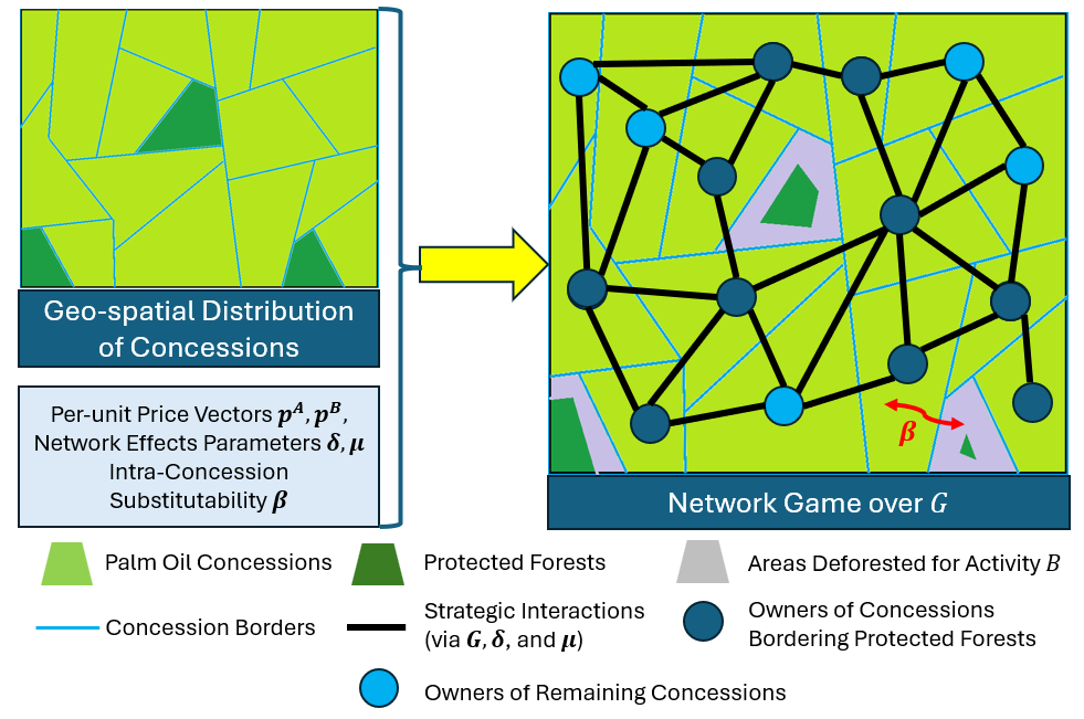
Figure 1: Illustration of our game-theoretic setup. We distinguish between the owners of concessions that share borders with protected forests and the rest of the concession owners in order to emphasize that the former category of owners are likely to have lower costs of unsustainable production because of their geographical proximity to protected forests.

On the basis of (1), our intervention design problems $P_{1}$ and $P_{2}$ can be stated precisely as follows, where the subscript ₀ refers to the pre-intervention scenario.

1. Minimize the aggregate unsustainable effort (i.e., the sum of all the agents’ effort levels in activity $B$) subject to the following constraints: (i) no agent’s sustainable effort (i.e., effort in activity $A$) drops below her pre-intervention effort level, and (ii) the post-intervention per-unit prices of sustainable goods are no less than their pre-intervention counterparts and no greater than a pre-defined maximum $p_{\max}$. $P_{1}$ can be expressed compactly as

   Minimize $$\sum_{i=1}^{n}x_{i}^{B}$$ (3)

   $$\text{s.t.}\quad x_{i}^{A} \geq x_{i0}^{A}\quad\text{for all }i\in[n],$$ (4)

   $$p_{i}^{A} \geq p_{i0}^{A}\quad\text{for all }i\in[n],$$ (5)

   $$p_{i}^{A} \leq p_{\max}\quad\text{for all }i\in[n].$$ (6)

2. Maximize the social welfare (defined as the sum of all the agents’ net payoffs or utilities) of the network while ensuring that (i) the aggregate unsustainable effort remains below a user-defined tolerance $x_{\max}^{B}$, and (ii) the post-intervention per-unit prices of sustainable goods are no less than their pre-intervention counterparts and no greater than a pre-defined maximum $p_{\max}$. $P_{2}$ can be compactly expressed as

   Maximize $$\sum_{i=1}^{n}u_{i}\left(x^{A},x^{B}\right)$$ (7)

   $$\text{s.t.}\quad\sum_{i=1}^{n}x_{i}^{B} \leq x^{B}_{\max},$$ (8)

   $$p_{i}^{A} \geq p_{i0}^{A}\quad\text{for all }i\in[n],$$ (9)

   $$p_{i}^{A} \leq p_{\max}\quad\text{for all }i\in[n].$$ (10)

Note that both these problems have as their decision variables the agent-dependent per-unit prices $\{p_{i}^{A}:i\in[n]\}$ of goods produced as a result of activity $A$. $P_{1}$ seeks to maximally suppress the prevalence of unsustainable harvesting and manufacturing activities without accounting for the potential effects of such suppression on the aggregate payoff of all the agents (i.e., social welfare), whereas $P_{2}$ seeks to maximize this aggregate payoff while keeping the prevalence of unsustainable production below a threshold inputted as a problem parameter. $P_{1}$ is more relevant to scenarios in which deforestation rates have already reached alarming proportions and therefore need to be decimated at any cost, whereas $P_{2}$ is more relevant to scenarios in which sustainability is of value but the overall economic well-being of concession owners is considered paramount.

It is important to note that our intervention design problems $P_{1}$ and $P_{2}$ have only $\{p_{i}^{A}:i\in\{1,2,\ldots,n\}\}$ (and not $\{p_{i}^{B}:i\in\{1,2,\ldots,n\}\}$) as the decision variables.

Assumptions on Model Parameters

We begin with the simplest assumption.

Assumption 1.

We have $\mu>0$ and $\delta>0$.

In other words, the contributions of both cross-activity and intra-activity network effects are non-negative and non-decreasing in the agents’ effort levels, which is a consequence of our modeling assumption that all strategic interactions between the agents involve complementarities because the agents cooperate and share resources with their neighbors.

On the other hand, we assume that the contributions of intra-concession cross-activity effects are non-positive and non-increasing, because every agent has a finite capital and limited resources that she must divide between $A$ and $B$. This makes the agent’s individual effort levels substitutable across the two activities, or equivalently, we make the following assumption in our setup.

Assumption 2.

We have $\beta>0.$

Next, we assume that the network effects parameters $\delta$ and $\mu$ are small enough for [11, Assumption 3] to hold, which guarantees the existence of a unique Nash equilibrium while ensuring that network effects are not large enough to induce oscillations in the best-response dynamics (see [12] for an in-depth explanation). We reproduce this assumption below.

Assumption 3.

([11, Assumption 3]). We have $\max\left(\frac{|\delta+\mu|}{1+\beta},\frac{|\delta-\mu|}{1-\beta}\right)\lambda_{1}({G})<1$, where $\lambda_{1}(G)$ denotes the spectral radius of $G$.

Next, we assume the following.

Assumption 4.

We have $\mu<\delta$.

This means that cross-activity network effects are weaker than intra-activity network effects, which models the real-world scenario in which agents whose harvesting and manufacturing practices are largely sustainable try to avoid cooperating with those whose practices are largely unsustainable.

Finally, we make the following standard connectivity assumption on the network, which has $G$ as its (weighted) adjacency matrix.

Assumption 5.

The network is connected and undirected. Equivalently, $G$ is irreducible and symmetric.

Comparison with Prior Works

Our work is a contribution to the literature on intervention design for network games. However, unlike this paper, most of this literature (barring the few works discussed in the paragraphs below) has so far focused on single-activity games. One of the first seminal papers in this category is [13], which studies a linear best-response network game and solves the problem of identifying the “key player” – the agent whose removal from the network causes the aggregate effort level to decrease the most. There, it is shown that the solution to this problem gives rise to a novel measure of node centrality called intercentrality, and the key player is precisely the player with the greatest intercentrality in the network. More recently, [14] consider a similar model of a network game with quadratic utilities and studied the problem of maximizing the social welfare over the space of all possible network topologies. The main result therein is that the optimal network necessarily belongs to a class of graphs called nested split graphs. The recent work [15] generalizes these results to the case of networks modeled as directed graphs and shows that, under mild assumptions, the optimal networks in this case are hierarchical.

The interventions designed in all of the above works lie in the category of network interventions, i.e., the interventions are aimed at achieving the planner’s objective by altering the structure of the strategic interactions network. On the other hand, our work lies in the category of characteristic interventions [16] or interventions that seek to achieve the planner’s objective by modifying the agent characteristics (such as marginal utilities) rather than the network structure. This body of works includes [17], which studies a budget-constrained problem of maximizing the aggregate action in a single-activity network game by enhancing the availability of resources to the agents. It provides explicit expressions for the planner’s strategies in the case of linear best responses and also analyzes the case of nonlinear best responses. A recent paper in this line of works is [18], which considers network games with both linear and non-linear best responses and solves the problem of maximizing social welfare subject to quadratic cost adjustment constraints and uses “standalone marginal utilities” (the component of marginal returns that does not depend on the network topology) as the optimization variables. One of the main insights of [18] is that the desired (optimal) interventions are determined by the eigenvectors of the graph adjacency matrix. As our work, too, considers the problem of maximizing social welfare, it is closely related to [18] but differs from the latter in the crucial respect that we borrow a coupled-activity network game model from [11] to incorporate cross-activity and intra-activity network effects. Moreover, our intervention design problem also incorporates optimization constraints that vary across the two activities. It is also worth noting that [16] unifies the two lines of work – those that study network interventions with those that study characteristic inteventions – by considering games with quadratic utility functions and showing that every network intervention is equivalent to a characteristic intervention in the sense that there exists a characteristic intervention that yields the same post-intervention Nash equilibria as the network intervention in question. However, [16], too, focuses on the single-activity case unlike our present work.

It is important to clarify that we are not the first to study intervention design problems for network games that model agent participation in multiple activities. The recent work [19] considers the closely related problem of maximizing social welfare in a network game involving an arbitrary number of interdependent activities subject to quadratic price adjustment constraints. It provides explicit closed-form expressions for price adjustments that are asymptotically optimal in the limit as the price adjustment budget approaches either zero or infinity. There are, nevertheless, two major differences between our work and [19]. First, we impose both lower bound and upper bound constraints on the post-intervention per-unit prices rather than just a single quadratic constraint. This enables us to consider a wider range of price adjustment budgets rather than just the limiting cases of vanishingly small or infinite budgets. Second, our intervention design problems provide different treatments to the two different activities appearing in our game-theoretic setup by imposing different constraints on the effort levels of the agents in these activities. This is because our ultimate goal is only to suppress one of these activities, namely the unsustainable activity.

2 Main Results

In this section, we solve both the intervention design problems ($P_{1}$ and $P_{2}$), interpret the resulting optimal policies, and explain their significance for sustainable forestry.

We first consider $P_{1}$. As our goal is to find a pricing policy that achieves a positive reduction in the aggregate unsustainable equilibrium effort, there should exist at least one policy that is feasible and strictly outperforms the current policy. This motivates the following definition.

Definition 1 (Essential Feasibility).

For $i\in\{1,2\}$, we say that $P_{i}$ is essentially feasible if the feasible set of $P_{i}$ contains at least one policy $p^{A}$ for which $\sum_{i=1}^{n}x_{i}^{B}<\sum_{i=1}^{n}x_{i0}^{B}$. If $P_{i}$ is not essentially feasible, we say that it is essentially infeasible.

We now define the notation that we will use to characterize $P_{1}$ and $P_{2}$. We reproduce the definitions of the following scaled Leontief matrices from [11]:

$$M^{+} :=((1+\beta)I-(\delta+\mu)G)^{-1}$$

$$M^{-} :=((1-\beta)I-(\delta-\mu)G)^{-1}.$$

The existence of $M^{+}$ and $M^{-}$ is implied by Assumption 3. In addition, we let $b^{+}:=M^{+}\mathbf{1}$ and $b^{-}:=M^{-}\mathbf{1}$. We also let $d_{\min}:=\min_{i\in[n]}\sum_{j=1}^{n}g_{ij}$ denote the minimum weighted node degree of the network.

We now state our first main result: the solution to $P_{1}$.

Proposition 1.

The following statements hold true for $P_{1}$.

1. For all $G$, $\beta$, $\delta$, and $\mu$ satisfying Assumptions 1 - 4, $P_{1}$ is essentially feasible if $\mu<\beta\delta$ and essentially infeasible if $\mu>\max\{\frac{2\beta}{1+\beta^{2}}\delta,\frac{\beta}{d_{\min}}\}$.

2. Suppose $\mu<\beta\delta$. Then there exists a threshold

   $$p_{\max}^{*}:=\frac{(b^{-}+b^{+})^{\top}p^{B}}{(b^{-}-b^{+})^{\top}\mathbf{1}}=\frac{(b^{-}+b^{+})^{\top}p^{B}}{b_{\Delta}^{\top}\mathbf{1}}$$ (11)

   such that the optimal solution of $P_{1}$ satisfies the following:

   1. If $p_{\max}\leq p_{\max}^{*}$, then we have $p_{i}^{A}=p_{\max}$ for all $i\in[n]$.

   2. If $p_{\max}>p_{\max}^{*}$, then every $p^{A}$ satisfying $p_{\max}^{*}\leq p_{i}^{A}\leq p_{\max}$ for all $i\in[n]$ is optimal. In addition, $x_{i}^{B}=0$ for all $i\in[n]$.

Proof.

1. We first observe from [11, Theorem 4] that $P_{1}$ can be expressed as follows.

   $$\textbf{$P_{1}$:}\quad\text{Minimize }(b^{+}-b^{-})^{\top}z$$

   $$\text{ s.t. }\left(M^{+}+M^{-}\right)z \geq 2x_{0}^{A}-(M^{+}-M^{-})p^{B},$$ (12)

   $$z \geq p^{A}_{0}$$ (13)

   $$z \leq p_{\max}\mathbf{1},$$ (14)

   where $z=p^{A}$ is the vector of optimization variables (the post-intervention effective prices for activity $A$), and constraints (12), (13), and (14) are equivalent to (4), (5) and (6), respectively.

   To establish the essential feasibility of $P_{1}$ for $\mu<\beta\delta$, we first claim that ${B_{\Delta}:=M^{-}-M^{+}}$ is entry-wise positive. To prove this claim, we observe that

   $$B_{\Delta} =(1-\beta)^{-1}(I-(1-\beta)^{-1}(\delta-\mu)G)^{-1}-(1+\beta)^{-1}(I-(1+\beta)^{-1}(\delta+\mu)G)^{-1}$$

   $$\stackrel{{\scriptstyle(a)}}{{\geq}}(1-\beta)^{-1}(I-(1-\beta)^{-1}(\delta-\mu)G)^{-1}-(1-\beta)^{-1}(I-(1+\beta)^{-1}(\delta+\mu)G)^{-1}$$

   $$\stackrel{{\scriptstyle(b)}}{{=}}(1-\beta)^{-1}\sum_{k=0}^{\infty}\left(\left(\frac{\delta-\mu}{1-\beta}\right)^{k}-\left(\frac{\delta+\mu}{1+\beta}\right)^{k}\right)G^{k},$$

   where $(a)$ holds because $\beta>0$ and $(b)$ follows from Neumann series expansion [20, 5.6.$P_{2}$6], which converges due to Assumption 3. Now, we know from Assumption 5 that $G$ is the non-negative adjacency matrix of a graph in which there exists a walk from every node $i\in[n]$ to every other node $j\in[n]\setminus\{i\}$. This implies the following: for every pair $(i,j)\in[n]\times[n]$, there exists a $k_{ij}\in\mathbb{N}$ such that $(G^{k})_{ij}>0$ for $k=k_{ij}$ (which for $i=j$ implies that there exists a walk from $i$ to itself via another node $\ell\in[n]\setminus\{i\}$). Therefore, it suffices to show that the coefficient of $G^{k}$ in the above series expansion is positive for each $k\in\mathbb{N}$. To this end, we observe upon some simplification that $\mu<\beta\delta$ implies $(1-\beta)^{-1}(\delta-\mu)>(1+\beta)^{-1}(\delta+\mu)$. As a result, $(1-\beta)^{-k}(\delta-\mu)^{k}>(1+\beta)^{-k}(\delta+\mu)^{k}$ for all $k\in\mathbb{N}$. This completes the proof of the claim that $B_{\Delta}$ is positive.

   Therefore, the objective function $(b^{+}-b^{-})^{\top}z=-\mathbf{1}^{\top}B_{\Delta}^{\top}z$ is decreasing in every entry of $z$. It now follows from [11, Theorem 4] that $2\sum_{i=1}^{n}x_{i}^{B}=(b^{+}-b^{-})^{\top}p^{A}+\mathbf{1}^{\top}(M^{+}+M^{-})p^{B}$ is decreasing in each entry of $p^{A}=z$. Moreover, as all Leontief matrice are positive, $M^{+}+M^{-}$, which is the sum of two scaled Leontief matrices with positive scaling factors, is also positive. Therefore, any price vector $z$ that satisfies $p_{0}^{A}<z<p_{\max}\mathbf{1}$ also satisfies (12) - (14). Such a $z$ ensures that $2\sum_{i=1}^{n}x_{i}^{B}<(b^{+}-b^{-})^{\top}p_{0}^{A}+\mathbf{1}^{\top}(M^{+}+M^{-})p^{B}=2\sum_{i=1}^{n}x_{0i}^{B}$. Hence, $P_{1}$ is essentially feasible.

   Suppose now that $\mu>\max\{\frac{2\beta}{1+\beta^{2}}\delta,\frac{\beta}{d_{\min}}\}$. As $\beta<1$, we can use $\mu>\frac{2\beta\delta}{1+\beta^{2}}$ to verify that the inequality $\frac{(\delta+\mu)^{k}}{(1+\beta)^{k+1}}-\frac{(\delta-\mu)^{k}}{(1-\beta)^{k+1}}>0$ holds for all $k\in\mathbb{N}$. On the other hand, we know from the definition of $d_{\min}$ that $G\mathbf{1}\geq d_{\min}\mathbf{1}$. Using induction, this can be generalized to $G^{k}\mathbf{1}\geq d_{\min}^{k}\mathbf{1}$ for all $k\geq 1$. Consequently, using Neumann series expansions of $M^{+}$ and $M^{-}$ yields

   $$B_{\Delta}\mathbf{1} =\frac{2\beta}{1-\beta^{2}}\mathbf{1}-\sum_{k=1}^{\infty}\left(\frac{(\delta+\mu)^{k}}{(1+\beta)^{k+1}}-\frac{(\delta-\mu)^{k}}{(1-\beta)^{k+1}}\right)G^{k}\mathbf{1}$$

   $$\leq\frac{2\beta}{1-\beta^{2}}\mathbf{1}-\sum_{k=1}^{\infty}\left(\frac{(\delta+\mu)^{k}}{(1+\beta)^{k+1}}-\frac{(\delta-\mu)^{k}}{(1-\beta)^{k+1}}\right)d_{\min}^{k}\mathbf{1}$$

   $$\stackrel{{\scriptstyle(a)}}{{=}}\frac{2\beta}{1-\beta^{2}}\mathbf{1}-\frac{(\delta+\mu)d_{\min}}{(1+\beta)^{2}(1-(1+\beta)^{-1}(\delta+\mu)d_{\min})}\mathbf{1}+\frac{(\delta-\mu)d_{\min}}{(1-\beta)^{2}(1-(1-\beta)^{-1}(\delta-\mu)d_{\min})}\mathbf{1},$$

   where $(a)$ follows from Geometric series expansion. On simplification, the above inequality reduces to $B_{\Delta}\mathbf{1}\leq-c_{0}(2\beta d_{\min}^{2}(\delta^{2}-\mu^{2})+(1-\beta^{2})(d_{\min}\mu-\beta))\mathbf{1}$ for some $c_{0}>0$. It now follows from Assumption 4 and $\mu\geq\frac{\beta}{d_{\min}}$ that $B_{\Delta}\mathbf{1}\leq 0$, i.e., $b^{+}-b^{-}\geq 0$. Therefore, the value of the objective function is non-decreasing in every entry of $z$, and hence, (13) implies that the objective function is minimized at $p_{0}^{A}$. In other words, $P_{1}$ is essentially infeasible.

2. We know from [11, Theorem 4] that $z=p^{*}_{\max}\mathbf{1}$ implies $2\sum_{i=1}^{n}{x_{i}^{B}}=-(b^{-}-b^{+})^{\top}\mathbf{1}p_{\max}^{*}-(b^{-}+b^{+})^{\top}p^{B}=0$. Thus, if $p_{\max}>p_{\max}^{*}$, then in view of our preceding observation that the objective function is non-increasing in $z$, every value of $z$ satisfying $p_{\max}^{*}\mathbf{1}\leq z\leq p_{\max}\mathbf{1}$ is optimal because it drives the aggregate unsustainable equilibrium effort to 0. On the other hand, if $p_{\max}<p_{\max}^{*}$, then the optimal solution is attained at the upper bound on $z$ specified by (14) because the objective function is decreasing in $z$ by virtue of $B_{\Delta}$ being positive (as proved above).

Assertion 1 provides a set of necessary conditions and also a set of sufficient conditions for the essential feasibility of $P_{1}$. Taken together, these conditions mean the following: for us to be able to reduce the aggregate unsustainable activity $\sum_{i}x_{i}^{B}$ in the network without decreasing the agents’ sustainable effort levels with respect to their pre-intervention values $\{x_{0i}^{A}\}_{i=1}^{n}$ and without decreasing the per-unit prices of sustainable goods w.r.t. their pre-intervention counterparts $\{p_{0i}^{A}\}_{i=1}^{n}$, the cross-activity network effects (quantified by $\mu$) must not exceed the combined effect of the intra-activity network effects (quantified by $\delta$) and the intra-concession substitutability (quantified by $\beta$ and the function $\max\{\frac{2\beta}{1+\beta^{2}}\delta,\frac{\beta}{d_{\min}}\}$, which is increasing in $\beta$ on $(-1,1)$) across the two activities.

To explain these conditions intuitively, we first note that increasing the per-unit price of sustainable goods for any agent increases the agent’s incentive to produce sustainably, which further increases the incentive of the agent’s neighbors to produce sustainably (via the network $G$ and the intra-activity network effects parameter $\delta$). This increase has two conflicting effects on the agents’ incentives to engage in unsustainable production: (a) via $\beta$ (intra-concession substitutability), it decreases the incentive to produce unsustainably (i.e., as the agents increase their participation in sustainable production, their cost of dividing effort and resources between the two activities compels them to decrease their participation in unsustainable production), and (b) via cross-activity agent-to-agent complementarities, it increases the incentive to produce unsustainably. To minimize the aggregate unsustainable activity, we need to ensure that the former effect (a) dominates over the latter effect (b), and this is made precise by the conditions in Assertion 1.

Note that the necessary and sufficient conditions provided by Assertion 1 are not tight. This is because for $\mu\in\left(\beta\delta,\max\{\frac{2\beta}{1+\beta^{2}}\delta,\frac{\beta}{d_{\min}}\}\right)$, the feasibility of $P_{1}$ depends on the structure of the network (as captured by $G$) and the values of $\delta$ and $\beta$.

Next, observe that Assertion 2 requires all the post-intervention per-unit prices of sustainable goods to equal the maximum allowable price $p_{\max}$ when this price is below the threshold $p_{\max}^{*}$. This is because the assumption $\mu<\beta\delta$ guarantees that the post-intervention unsustainable effort levels $\{x_{i}^{B}\}_{i=1}^{n}$ are monotonically non-increasing in every per-unit price $p_{i}^{A}$, and in particular, $\{x_{i}^{B}\}_{i=1}^{n}$ are monotonically decreasing in $\{p_{i}^{A}\}_{i=1}^{n}$ when $p_{\max}<p_{\max}^{*}$. However, as $p_{\max}$ crosses the threshold $p_{\max}^{*}$, the aggregate unsustainable activity $\sum_{i=1}^{n}x_{i}^{B}$ vanishes in the post-intervention equilibrium, which means that increasing the per-unit prices beyond $p_{\max}^{*}$ does not yield any additional benefit over setting all of them to $p_{\max}^{*}$. Nevertheless, as there is no undesirable effect of increasing $p_{i}^{A}$ beyond $p_{\max}$, there exists a range of optimal prices for the case $p_{\max}>p_{\max}^{*}$.

Remark 1.

It is easy to verify that $b^{-}+b^{+}$ captures the sensitivity of the aggregate unsustainable activity $\sum_{i=1}^{n}x_{i}^{B}$ to the per-unit prices of unsustainable goods, i.e., every unit increase in $p_{i}^{B}$ raises $\sum_{i=1}^{n}x_{i}^{B}$ by $b_{i}^{-}+b_{i}^{+}$. On the other hand, $b^{-}-b^{+}$ is the sensitivity of $\sum_{i=1}^{n}x_{i}^{B}$ to the per-unit prices of sustainable goods, i.e., every unit increase in $p_{i}^{A}$ reduces $\sum_{i=1}^{n}x_{i}^{B}$ by $b_{i}^{-}-b_{i}^{+}$. Hence, (11) implies that the threshold on the maximum price $p_{\max}^{*}$ depends on the sensitivities of the aggregate unsustainable activity to the per-unit prices of both sustainable and unsustainable goods. In the special case of uniform pricing (wherein the per-unit prices of both kinds of goods are homogeneous across the agents), it follows that $p_{\max}^{*}$ is proportional to the per-unit price of unsustainable goods with the constant of proportionality being the ratio of the sensitivities of the aggregate unsustainable activity to $p^{B}$ and $p^{A}$).

Remark 2.

Observe from the relation $2\sum_{i=1}^{n}x_{i}^{B}=(b^{+}-b^{-})^{\top}p^{A}+(b^{+}+b^{-})^{\top}p^{B}$ (which is a straightforward consequence of  [11, Theorem 4]) that the aggregate unsustainable activity $\sum_{i=1}^{n}x_{i}^{B}$ is more sensitive to increases in $p_{i}^{A}$ for higher values of $b_{\Delta i}=b_{i}^{-}-b_{i}^{+}$. This leads to an interpretation of $b_{\Delta}$ as a vector of node centralities: agents with higher values of $b_{\Delta i}$ are more central in the network in the sense that they are better-positioned than other agents for the purpose of transferring the unsustainability-suppressing effects of their individual price interventions to the rest of the network. Furthermore, the entry-wise positivity of $B_{\Delta}$ implies the entry-wise positivity of $b_{\Delta}$, which means that the centralities of interest are all positive as a consequence of Assumption 5.

Our next goal is to solve $P_{2}$ and state the resulting welfare-maximizing policy. We first remark that $P_{2}$ can be verified to be essentially feasible if $\mu<\beta\delta$, $p_{\max}$ is large enough (as made precise in Proposition 2) and $x_{\max}^{B}<\sum_{i=1}^{n}x_{i0}^{B}$, i.e., if our price adjustment budget is high and our tolerance for the aggregate unsustainable effort is lower than its value at the pre-intervention equilibrium.

Next, we define the required notation and evaluate the required quantities. We let $k_{0}:=\mathbf{(}b^{+}+b^{-})^{\top}p^{B}-2x_{\max}^{B}$, and evaluate the social welfare at the post-intervention equilibrium by plugging in the expressions for equilibrium effort levels provided in [11, Theorem 4] into the utility expression (1). This yields

$$\sum_{i=1}^{n}u_{i}\left(x^{A},x^{B}\right)=z^{\top}Qz-v^{\top}z,$$ (15)

where $z:=p^{A}$ is the vector of optimization variables,

$$\begin{split}Q:={M}^{+}\left(2I-(1+\beta){M}^{+}+2(\delta+\mu){M}^{+}G\right)+{M}^{-}\left(2I-(1-\beta){M}^{-}+2(\delta-\mu){M}^{-}G\right),\end{split}$$

and $v:=-Rp^{B}$, where

$$\begin{split}R:={M}^{+}\left(2I-(1+\beta){M}^{+}+2(\delta+\mu){M}^{+}G\right)-{M}^{-}\left(2I-(1-\beta){M}^{-}+2(\delta-\mu){M}^{-}G\right).\end{split}$$

On the basis of (15), we say that between two candidate pricing policies $z,\tilde{z}\in\mathbb{R}^{n}_{\geq 0}$, the policy $\tilde{z}$ is more welfare-enhancing than $z$ if $\tilde{z}^{\top}Q\tilde{z}-v^{\top}\tilde{z}>z^{\top}Qz-v^{\top}z$, i.e., if $\tilde{z}$ results in a higher social welfare.

Furthermore, we use the equilibrium characterization in [11, Theorem 4] to express (8) as $\left(b^{-}-b^{+}\right)^{\top}z\geq k_{0}$. As a result, $P_{2}$ can be expressed as

$$P_{2}\textbf{:}\quad\text{Maximize }z^{\top}Qz -v^{\top}z$$ (16)

$$\text{ s.t. }\quad b_{\Delta}^{\top} z\geq k_{0}$$ (17)

$$z\geq p^{A}_{0}$$ (18)

$$z\leq p_{\max}\mathbf{1}.$$ (19)

On this basis, we have the following result, which shows that a generic characterization of the solution of $P_{2}$ is abstract and inefficient to compute owing to the well-known NP-hardness of convex maximization problems.

Proposition 2.

Suppose $\mu<\beta\delta$, $x_{\max}^{B}<\sum_{i=1}^{n}x_{i0}^{B}$, and $2Qp_{0}^{A}<v$. Then the solution of $P_{2}$ is given by $p^{A}=p_{\max}\mathbf{1}$ if $p_{0}^{A}\geq\frac{1}{2}p^{B}$. Moreover, the following assertions are true when the constraint (17) is dropped.

1. There exists a threshold $p_{\max}^{(1*)}$ on $p_{\max}$ such that if $p_{\max}\geq p_{\max}^{(1*)}$, the solution to $P_{2}$ is given by $p_{i}^{A}=p_{\max}$ for all $i\in[n]$. Moreover, $p_{\max}^{(1*)}$ is given by

   $$p_{\max}^{(1*)}:=\max_{S\subset[n]}\max_{i\in[n]}\left\{\frac{v_{i}-\sum_{j\in S}q_{ij}p_{0j}^{A}}{2(Q\mathbf{1})_{i}-\sum_{j\in S}q_{ij}}\right\}.$$

2. There exists another threshold $p_{\max}^{(2*)}$ on $p_{\max}$ such that if $p_{\max}^{(2*)}<p_{\max}<p_{\max}^{(1*)}$, then the optimal solution of $P_{2}$ is $z^{*}$, which is defined as

   $$z_{i}^{*}:=\begin{cases}p_{0i}^{A}\quad&\text{if }i\in S^{*}\\ p_{\max}\quad&\text{if }i\in[n]\setminus S^{*},\end{cases}$$

   where

   $$S^{*}:=\operatornamewithlimits{argmax}_{S\subset[n]}\max_{i\in[n]}\left\{\frac{v_{i}-\sum_{j\in S}q_{ij}p_{0j}^{A}}{2(Q\mathbf{1})_{i}-\sum_{j\in S}q_{ij}}\right\}.$$

3. If $p_{0}^{A}=Q^{-1}|R|p^{B}-\alpha\mathbf{1}=Q^{-1}v-\alpha\mathbf{1}$ for some $\alpha>0$ and if $v>\left(I+\frac{1}{\min_{i,j\in[n]}q_{ij}}\emph{diag}(Q\mathbf{1})\right)Qp_{0}^{A}$, then for $p_{\max}^{(2*)}\leq p_{\max}<p_{\max}^{(1*)}$, the optimal solution of $P_{2}$ is $z^{*}=p_{0}^{A}$.

Proof.

We solve $P_{2}$ by establishing that $Q$ is positive-definite and finding appropriate functional forms for $Q$ and $R$.

Observe from the definitions of $M^{+}$ and $M^{-}$ that $Q=f(G)$, where $f$ is defined by

$$f(A) =h^{+}(A)(2I-(1+\beta)h^{+}(A)+2(\delta+\mu)h^{+}(A)A)+h^{-}(A)(2I-(1-\beta)h^{-}(A)+2(\delta-\mu)h^{-}(A)A),$$

with $h^{+}(A):=((1+\beta)I-(\delta+\mu)A)^{-1}$ and $h^{-}(A):=((1-\beta)I-(\delta-\mu)A)^{-1}$ for all $A\in\mathbb{R}^{n\times n}$.

Therefore, the eigenvalues of $Q$ are given by $\{f(\lambda_{i}):i\in[n]\}$, where $\{\lambda_{i}:i\in[n]\}$ are the eigenvalues of $G$ [21, (7.3.5)]. On simplification, this gives

$$f(\lambda_{i})=\frac{1+\beta}{(1+\beta-(\delta+\mu)\lambda_{i})^{2}}+\frac{1-\beta}{(1-\beta-(\delta-\mu)\lambda_{i})^{2}}>0$$

because $\beta\in(-1,1)$. Thus, all the eigenvalues of $Q$ are positive. As $Q$ is symmetric, it now follows that $Q$ is positive-definite. Moreover, the eigenvectors of $Q$ are the same as those of $G$ [21, (7.3.5)]. We can now verify that $Q$ has the same eigenvectors and eigenvalues as $(1+\beta)(M^{+})^{2}+(1-\beta)(M^{-})^{2}$, which is positive because (scaled) Leontief matrices associated with connected graphs (Assumption 5) are positive [22, Theorem 4.10]. As both $Q$ and $S$ are symmetric, it follows from the spectral decomposition theorem for diagonalizable matrices that

$$Q:=(1+\beta)(M^{+})^{2}+(1-\beta)(M^{-})^{2}.$$ (20)

Similarly, we can show that

$$R=(1+\beta)(M^{+})^{2}-(1-\beta)(M^{-})^{2}.$$ (21)

Using (20) and (21), the objective function can be expressed as

$$~{}\phi(z) =(1+\beta)(z+p^{B})^{\top}(M^{+})^{2}z+(1-\beta)(z-p^{B})^{\top}(M^{-})^{2}z,$$ (22)

which is increasing in $z$ for $z>p^{B}$. Therefore, if $p_{0}^{A}>p^{B}$, then (18), (19), and our assumption that $p_{\max}>\max_{i\in[n]}p_{i0}^{A}$ imply that $\phi(z)$ is maximized at $z=p_{\max}\mathbf{1}$.

On the other hand, for $p_{0}^{A}<p^{B}$ we define $y:=z-\frac{p^{B}}{2}$, substitute for $z$ in (22), and use the property that $M^{\pm}=(M^{\pm})^{\top}$ to express the $P_{2}$ in terms of $y$ as

$$\text{Maximize}\quad\psi(y) :=(1+\beta)\left(y+\frac{3}{2}p^{B}\right)^{\top}(M^{+})^{2}\left(y+\frac{1}{2}p^{B}\right)+(1-\beta)y^{\top}(M^{-})^{2}y$$

$$\text{s.t.}\quad b_{\Delta}^{\top}y \geq k_{0}-\frac{1}{2}b_{\Delta}^{\top}p^{B}$$ (23)

$$y \geq p_{0}^{A}-\frac{p^{B}}{2}$$ (24)

$$y \leq p_{\max}\mathbf{1}-\frac{p^{B}}{2}.$$ (25)

As the scaled Leontief matrices $M^{+}$ and $M^{-}$ are positive and $\beta\in(0,1)$ (Assumption 2), the function $\psi(y)$ is increasing in every entry of $y$ for $y\geq\mathbf{0}$. Moreover, as argued in the proof of Proposition 1, $\mu<\beta\delta$ implies $b_{\Delta}>\mathbf{0}$. Therefore, increasing $y$ does not lead to the violation of (24), and as a result, the optimal solution is obtained at the extreme point determined by (25), i.e., $y^{*}=p_{\max}\mathbf{1}-p^{B}/2$. Equivalently, when $z\geq p^{B}/2$ is an implicit constraint, we have $z^{*}=p_{\max}\mathbf{1}$. This proves the assertion that $z=p_{\max}\mathbf{1}$ is an optimal policy when $p_{0}^{A}\geq p^{B}/2$.

For the rest of the proof, recall the positive-definiteness of $Q$ established in the preceding arguments. This property implies that $P_{2}$ seeks to maximize a strongly convex objective function over a polytope. Hence, an optimal solution of $P_{2}$ can be found at an extreme point of the polytope $\mathcal{P}$ defined by (17) - (19).

We now prove Assertions 1 and 2 and omit the proof of Assertion 3 since it follows similar arguments.

1. Due to the positive-definiteness of $Q$, the function $\phi(z):=z^{\top}Qz-v^{\top}z$ is unbounded on $\mathbb{R}_{+}^{n}$ and increasing in each entry of $z$ for sufficiently large values of the entries (since its gradient is $\nabla\phi(z)=2Qz-v$ due to the symmetry of $Q$). It follows from (19) that $P_{2}$ is maximized at $z=p_{\max}\mathbf{1}$ for sufficiently large values of $p_{\max}$. However, $R$ being negative implies that $v=-Rp^{B}>0$, which in turn implies that for sufficiently small values of the entries of $z$, we have $2Qz-v<0$ (which is possible because $2Qp_{0}^{A}<v$), and hence, there exists a threshold on $\max_{i}z_{i}$ below which $\phi(z)$ decreases in every entry of $z$. It follows that there exists a $p_{\max}^{(1*)}>0$ such that the extreme point $p_{\max}\mathbf{1}$ is optimal if and only if $p_{\max}\geq p_{\max}^{(1*)}$.

   To compute $p_{\max}^{(1*)}$, we first obtain a necessary and sufficient condition for $p_{\max}\mathbf{1}$ to be an optimal solution. Note that we only need to compare $p_{\max}\mathbf{1}$ with other extreme points of $\mathcal{P}$. As $p_{\max}\mathbf{1}$ is an entry-wise upper bound on every extreme point of $\mathcal{P}$, we can set $z=p_{\max}\mathbf{1}$ and use Lemma 1 (see the appendix) to compare $z$ with other extreme point policies, all of which are of the form $z-\Delta$ for $\Delta\geq\mathbf{0}$. Doing so results in the following observations: (a) for $p_{\max}\mathbf{1}$ to be a strictly sub-optimal solution, there must exist an extreme point $\tilde{z}=z-\Delta$ such that $2p_{\max}(Q\mathbf{1})_{i}-v_{i}<(Q\Delta)_{i}$ for some $i\in[n]$, and (b) if we have $2p_{\max}(Q\mathbf{1})_{i}-v_{i}<(Q\Delta)_{i}$ for some $i\in[n]$, then we know that $z-\Delta_{i}e^{(i)}$ is more welfare-enhancing than $z$ so long as $z-\Delta_{i}e^{(i)}$ is an extreme point of $\mathcal{P}$.

   We now consider policies of the form $z-\Delta_{i}e^{(i)}$ where $\Delta_{i}=p_{\max}-\bar{\Delta}$ for some $\bar{\Delta}\in(p_{0i}^{A},p_{\max})$ and $i\in[n]$. Note that this range of values of $\bar{\Delta}$ is both necessary and sufficient for feasibility (i.e., for $z-\Delta_{i}e^{(i)}\in\mathcal{P}$). For such policies, the condition $2p_{\max}(Q\mathbf{1})_{i}-v_{i}<(Q\Delta)_{i}$ reduces to $p_{\max}<\frac{v_{i}-q_{ii}\bar{\Delta}}{2(Q\mathbf{1})_{i}-q_{ii}}.$

   Therefore, there exists a feasible policy of the form $z-\Delta_{i}e^{(i)}$ that is more welfare-enhancing than $z=p_{\max}\mathbf{1}$ if and only if

   $$p_{\max}<\widetilde{p_{i}}:=\max_{j\in[n]}\max_{\bar{\Delta}\in(p_{0i}^{A},p_{\max})}\left\{\frac{v_{j}-q_{ii}\bar{\Delta}}{2(Q\mathbf{1})_{j}-q_{ji}}\right\}=\max_{j\in[n]}\left\{\frac{v_{j}-q_{ji}p_{0i}^{A}}{2(Q\mathbf{1})_{j}-q_{ji}}\right\}.$$ (26)

   Similarly, we can show that there cannot exist a feasible policy of the form $z-\sum_{j\in S}\Delta_{j}e^{(j)}$ that is more welfare-enhancing than $z=p_{\max}\mathbf{1}$ unless

   $$p_{\max}<\tilde{p}_{S}:=\max_{i\in S}\max_{\bar{\Delta}_{j}\in(p_{0j}^{A},p_{\max})}\left\{\frac{v_{i}-\sum_{j\in S}q_{ij}\bar{\Delta}_{j}}{2(Q\mathbf{1})_{i}-\sum_{j\in S}q_{ij}}\right\}=\max_{i\in S}\left\{\frac{v_{i}-\sum_{j\in S}q_{ij}p_{0j}^{A}}{2(Q\mathbf{1})_{i}-\sum_{j\in S}q_{ij}}\right\},$$ (27)

   and $z-\sum_{j\in S}(p_{\max}-p_{0j}^{A})$ is more welfare-enhancing than $z=p_{\max}\mathbf{1}$ if

   $$p_{\max}<\min_{i\in S}\left\{\frac{v_{i}-\sum_{j\in S}q_{ij}p_{0j}^{A}}{2(Q\mathbf{1})_{i}-\sum_{j\in S}q_{ij}}\right\}.$$ (28)

   It follows that $z=p_{\max}\mathbf{1}$ is not strictly sub-optimal unless $p_{\max}<p_{\max}^{(1*)}$.

2. If

   $$\max_{S\subset[n],S\neq S^{*}}\max_{i\in S}\left\{\frac{v_{i}-\sum_{j\in S}q_{ij}p_{0j}^{A}}{2(Q\mathbf{1})_{i}-\sum_{j\in S}q_{ij}}\right\}<p_{\max}<\min_{i\in S^{*}}\left\{\frac{v_{i}-\sum_{j\in S^{*}}q_{ij}p_{0j}^{A}}{2(Q\mathbf{1})_{i}-\sum_{j\in S^{*}}q_{ij}}\right\},$$

   then (27) does not hold for any feasible policy $z-\sum_{j\in S}\Delta_{j}e^{(j)}$ for which $S\neq S^{*}$. It follows from the preceding arguments that $z-\sum_{j\in S}\Delta_{j}e^{(j)}$ is not as welfare-enhancing as $p_{\max}\mathbf{1}$, and hence, $z-\sum_{j\in S}\Delta_{j}e^{(j)}$ cannot be an optimal solution of $P_{2}$ unless $S=S^{*}$. On the other hand, when $S=S^{*}$, then (28) implies that $z-\sum_{j\in S^{*}}(p_{\max}-p_{0j}^{A})e^{(j)}$ is optimal.

3. We infer from (27) that the policy $z-\sum_{j\in[n]}(p_{\max}-p_{0j}^{A})e^{(j)}=p_{0}^{A}$ is not more welfare-enhancing than $p_{\max}\mathbf{1}$ unless

   $$p_{\max}<\tilde{p}^{\uparrow}:=\max_{i\in[n]}\left\{\frac{v_{i}-(Qp_{0}^{A})_{i}}{(Q\mathbf{1})_{i}}\right\}.$$

   Likewise, we can use Lemma 1 to show that $p_{0}^{A}$ is more welfare-enhancing than $p_{\max}\mathbf{1}$ if

   $$p_{\max}<\tilde{p}_{\downarrow}:=\min_{i\in[n]}\left\{\frac{v_{i}-(Qp_{0}^{A})_{i}}{(Q\mathbf{1})_{i}}\right\}.$$

   On the other hand, observe that

   $$\frac{v_{i}-(Qp_{0}^{A})_{i}}{(Q\mathbf{1})_{i}}=\frac{v_{i}-(Q(Q^{-1}v-\alpha\mathbf{1}))_{i}}{(Q\mathbf{1})_{i}}=\alpha$$

   for all $i\in[n]$. It follows that $\tilde{p}^{\uparrow}=\tilde{p}^{\downarrow}$ and that $p_{0}^{A}$ is more welfare-enhancing than $p_{\max}\mathbf{1}$ if and only if

   $$p_{\max}<\frac{v_{i}-(Qp_{0}^{A})_{i}}{(Q\mathbf{1})_{i}}\quad\text{for any }i\in[n].$$ (29)

   Now, for any $S\subset[n]$ with $S\neq[n]$, we have the following for every $i\in[n]$:

   $$(Q\mathbf{1})_{i}\left(2(Q\mathbf{1})_{i}-\sum_{j\in S}q_{ij}\right)\left(\frac{v_{i}-(Qp_{0}^{A})_{i}}{(Q\mathbf{1})_{i}}-\frac{v_{i}-\sum_{j\in S}q_{ij}p_{0j}^{A}}{2(Q\mathbf{1})_{i}-\sum_{j\in S}q_{ij}}\right)$$

   $$=(Q\mathbf{1})_{i}v_{i}-\left(\sum_{j\in S}q_{ij}\right)v_{i}-((Q\mathbf{1})_{i}-\sum_{j\in S}q_{ij})(Qp_{0}^{A})_{i}-(Q\mathbf{1})_{i}\sum_{j\notin S}q_{ij}p_{0j}^{A}$$

   $$=\left(\sum_{j\notin S}q_{ij}\right)v_{i}-\left(\sum_{j\notin S}q_{ij}\right)\left(\sum_{j=1}^{n}q_{ij}p_{0j}^{A}\right)-(Q\mathbf{1})_{i}\left(\sum_{j\notin S}q_{ij}p_{0j}^{A}\right)$$

   $$=\left(\sum_{j\notin S}q_{ij}\right)\left(v_{i}-(Qp_{0}^{A})_{i}-\frac{1}{\sum_{j\notin S}q_{ij}}\sum_{j\notin S}q_{ij}p_{0j}^{A}\right)$$

   $$\stackrel{{\scriptstyle(a)}}{{>}}\left(\sum_{j\notin S}q_{ij}\right)\left(v_{i}-(Qp_{0}^{A})_{i}-\frac{1}{\sum_{j\notin S}q_{ij}}(Qp_{0}^{A})_{i}\right)$$

   $$\stackrel{{\scriptstyle(b)}}{{>}}\left(\sum_{j\notin S}q_{ij}\right)\left(v_{i}-\left(1+\frac{1}{\min_{i,j\in[n]}q_{ij}}\right)(Qp_{0}^{A})_{i}\right)$$

   $$\stackrel{{\scriptstyle(c)}}{{>}}0,$$

   where $(a)$ is a consequence of the non-negativity of $Q$ and $p_{0}^{A}$, $(b)$ follows from the non-negativity of $Q$, and $(c)$ holds because $v>\left(I+\frac{1}{\min_{i,j\in[n]}q_{ij}}\text{diag}(Q\mathbf{1})\right)Qp_{0}^{A}$. We also make the following observation: ${2(Q\mathbf{1})_{i}-\sum_{j\in S}q_{ij}=2\sum_{j\in[n]}q_{ij}-\sum_{j\in S}q_{ij}>0}$. Therefore,

   $$\frac{v_{i}-(Qp_{0}^{A})_{i}}{(Q\mathbf{1})_{i}}>\frac{v_{i}-\sum_{j\in S}q_{ij}p_{0j}^{A}}{2(Q\mathbf{1})_{i}-\sum_{j\in S}q_{ij}}$$

   for all $S\subset[n]$. Assertion 3 is now a straightforward consequence of Assertion 2.

Proposition 2 shows that, under certain assumptions, there exists a threshold $p_{\max}^{(1*)}$ such that when $p_{\max}$ exceeds this threshold, the optimal policy sets the per-unit price of every agent’s sustainable goods to $p_{\max}$. In this case, the intervention enables every agent to increase her net utility while either decreasing her effort level in the unsustainable activity or keeping it the same as before. This is possible because the post-intervention prices $p^{A}$ are high enough to ensure that the increased incentive to produce sustainably when combined with intra-concession substitutability between the two activities effectively disincentivizes unsustainable production while increasing (or preserving) social welfare.

When $p_{\max}<p_{\max}^{(1*)}$, there exists another threshold $p_{\max}^{(2*)}$ such that when $p_{\max}^{(2*)}<p_{\max}<p_{\max}^{(1*)}$, the optimal policy increases the per-unit price $p_{i}^{A}$ for a smaller number of agents.

Discussion and Ongoing work

We have designed two pricing policies by formulating and solving two budget-constrained optimization problems, namely, $P_{1}$, which seeks to maximally reduce the aggregate unsustainable activity in the post-intervention equilibrium, and $P_{2}$, which seeks to maximize social welfare while keeping the aggregate unsustainable activity below a pre-defined tolerance. We observe that the solutions of $P_{1}$ and $P_{2}$ are consistent with each other when the maximum allowable price exceeds the greatest among the identified thresholds (namely $p_{\max}^{*}$ for $P_{1}$ and $p_{\max}^{(1*)}$ for $P_{2}$). This means that when the price adjustment budget is sufficiently large, it is possible to eliminate the aggregate unsustainable activity entirely while simultaneously maximizing social welfare in a manner that makes no compromise on any agent’s sustainable production levels.

However, when $p_{\max}$ begins to fall below these thresholds, the solution of $P_{1}$ requires us to raise the per-unit prices of sustainable goods for all the $n$ agents in a contrast to the solution of $P_{2}$, which may require us to restrict the number of agents to which the intervention is applied. This is because a tight price-adjustment budget makes the goal of social welfare maximization conflict with that of the suppression of any one of the two activities. To elaborate, an insufficient price adjustment budget is unable to make the post-intervention effort levels in the unsustainable activity negligible in comparison with the post-intervention effort levels in the sustainable activity. Therefore, the intervention proposed by $P_{1}$ requires the agents to divide their resources more or less equitably between the two activities, and this results in the intra-concession substitutability ($\beta$) reducing the social welfare. In sum, low-budget scenarios lead to $P_{1}$ suppressing unsustainability at the expense of social welfare and $P_{2}$ maximizing social welfare while allowing unsustainability to reach the maximum tolerable levels.

We now compare our results with those reported in [19], which is the most closely related to our work. We reiterate that [19] only considers the goal of social welfare maximization whereas we consider both welfare maximization and the maximal suppression of any one activity. In addition, unlike [19], which characterizes the optimal policy only in the limits as the price adjustment budget goes to either zero or infinity, we consider a non-asymptotic budget and provide a case-wise characterization of the policy for all value ranges of the budget. Even if we restrict the comparison of both these works to welfare maximization under unbounded or vanishingly low budgets, we find that our optimal pricing policy differs remarkably from that derived in [19]: our policy keeps the agent prices as uniform as possible whereas the latter is characterized by the principal eigenvector of $G$ in the unbounded budget scenario and by the pre-intervention price vector in the vanishing budget scenario. This is because of two reasons. First, as mentioned before, our optimization constraints differ from those used in [19] since we are interested in keeping exactly one of the two activities in check, whereas the problem studied in [19] does not impose differential requirements on the activities. Second, our budget constraint is affine whereas the one used in [19] is quadratic, which explains the close relationship between their optimal policy with the principal eigenvector of $G$, which captures the network structure.

It would, nevertheless, be interesting to investigate the role of network structures typical of concession networks in the context of our setup. This requires a careful study of the real-world geospatial distributions of forest concessions, information on which can be obtained from datasets provided by Global Forest Watch and Greenpeace datasets [23, 24]. Such an empirical study is part of our ongoing work.

Specializing our theoretical results to network topologies inferred using empirical methods should provide useful insights on the characteristics of our optimal policies and their implications for owners whose plantations have different geographical positions relative to each other within the forest concessions network.

Appendix

Lemma 1.

Let $z\in\mathbb{R}^{n}_{\geq 0}$ be a pricing policy. Then, for any $\Delta\in\mathbb{R}^{n}{\geq 0}$, the policy $p^{A}=z-\Delta$ is more welfare-enhancing than $p^{A}=z$ if and only if

$$\Delta^{\top}(2Qz-v-Q\Delta)<0.$$

In particular, the existence of an index $i\in[n]$ such that $2(Qz)_{i}-v_{i}<(Q\Delta)_{i}$ is

1. necessary for the policy $p^{A}=z-\Delta$ to be more welfare-enhancing than the policy $p^{A}=z$, and

2. sufficient for the policy $p^{A}=z-\Delta_{i}e^{(i)}$ to be more welfare-enhancing than $p^{A}=z$ if $\Delta_{i}>0$.

Proof.

By (15), the policy $z-\Delta$ results in a higher social welfare if and only if

$$z^{\top}Qz-v^{\top}z<(z-\Delta)^{\top}Q(z-\Delta)-v^{\top}(z-\Delta),$$

which simplifies to $\Delta^{\top}(2Qz-v-Q\Delta)<0$. As $\Delta$ is non-negative, it follows that there exists at least one index $i\in[n]$ such that $2(Qz)_{i}-v_{i}<(Q\Delta)_{i}$. This establishes (i).

For (ii), note that setting $\Delta=\Delta_{i}e^{(i)}$ results in

$$\left(z^{\top}Qz-v^{\top}z\right)-\left((z-\Delta)^{\top}Q(z-\Delta)-v^{\top}(z-\Delta)\right)=\Delta^{\top}(2Qz-v-Q\Delta)=\Delta_{i}(2(Qz)_{i}-v_{i}-(Q\Delta)_{i})<0,$$

where the last inequality holds because $\Delta_{i}>0$. Thus, we have shown that $z$ is less welfare-enhancing than $z-\Delta=z-\Delta_{i}e^{(i)}$, which completes the proof.

References

- [1] P. Friedlingstein, M. W. Jones, M. O’Sullivan, R. M. Andrew, D. C. Bakker, J. Hauck, C. Le Quéré, G. P. Peters, W. Peters, J. Pongratz, et al., “Global carbon budget 2021,” Earth System Science Data, no. 4, 2022.
- [2] C. Balboni, A. Berman, R. Burgess, and B. A. Olken, “The economics of tropical deforestation,” Annual Review of Economics, vol. 15, pp. 723–754, 2023.
- [3] A. Rodrigues, H. Koeppl, H. Ohtsuki, and A. Satake, “A game theoretical model of deforestation in human–environment relationships,” Journal of theoretical biology, vol. 258, no. 1, pp. 127–134, 2009.
- [4] É. Filotas, I. Witté, N. Aquilué, C. Brimacombe, P. Drapeau, W. S. Keeton, D. Kneeshaw, C. Messier, and M.-J. Fortin, “Network framework for forest ecology and management,” in Boreal Forests in the Face of Climate Change: Sustainable Management, pp. 685–717, Springer, 2023.
- [5] E. Bürgi and C. Oberlack, “Breakout session: Impacts of the eudr on commodity-producing countries: How to establish partnerships for deforestation-free supply chains?,” 2023.
- [6] K. M. Carlson, R. Heilmayr, H. K. Gibbs, P. Noojipady, D. N. Burns, D. C. Morton, N. F. Walker, G. D. Paoli, and C. Kremen, “Effect of oil palm sustainability certification on deforestation and fire in indonesia,” Proceedings of the National Academy of Sciences, vol. 115, no. 1, pp. 121–126, 2018.
- [7] D. L. Gaveau, B. Locatelli, M. A. Salim, H. Yaen, P. Pacheco, and D. Sheil, “Rise and fall of forest loss and industrial plantations in borneo (2000–2017),” Conservation Letters, vol. 12, no. 3, p. e12622, 2019.
- [8] V. M. Carvalho and A. Tahbaz-Salehi, “Production networks: A primer,” Annual Review of Economics, vol. 11, pp. 635–663, 2019.
- [9] D. Acemoglu, A. Ozdaglar, and A. Tahbaz-Salehi, “Networks, shocks, and systemic risk,” tech. rep., National Bureau of Economic Research, 2015.
- [10] D. Acemoglu, U. Akcigit, and W. Kerr, “Networks and the macroeconomy: An empirical exploration,” Nber macroeconomics annual, vol. 30, no. 1, pp. 273–335, 2016.
- [11] Y.-J. Chen, Y. Zenou, and J. Zhou, “Multiple activities in networks,” American Economic Journal: Microeconomics, vol. 10, no. 3, pp. 34–85, 2018.
- [12] Y. Bramoullé, R. Kranton, and M. D’amours, “Strategic interaction and networks,” American Economic Review, vol. 104, no. 3, pp. 898–930, 2014.
- [13] C. Ballester, A. Calvó-Armengol, and Y. Zenou, “Who’s who in networks. wanted: The key player,” Econometrica, vol. 74, no. 5, pp. 1403–1417, 2006.
- [14] M. Belhaj, S. Bervoets, and F. Deroïan, “Efficient networks in games with local complementarities,” Theoretical Economics, vol. 11, no. 1, pp. 357–380, 2016.
- [15] X. Li, “Designing weighted and directed networks under complementarities,” Games and Economic Behavior, vol. 140, pp. 556–574, 2023.
- [16] Y. Sun, W. Zhao, and J. Zhou, “Structural interventions in networks,” International economic review, vol. 64, no. 4, pp. 1533–1563, 2023.
- [17] G. Demange, “Optimal targeting strategies in a network under complementarities,” Games and Economic Behavior, vol. 105, pp. 84–103, 2017.
- [18] A. Galeotti, B. Golub, and S. Goyal, “Targeting interventions in networks,” Econometrica, vol. 88, no. 6, pp. 2445–2471, 2020.
- [19] R. Kor and J. Zhou, “Multi-activity influence and intervention,” Games and Economic Behavior, vol. 137, pp. 91–115, 2023.
- [20] R. A. Horn and C. R. Johnson, Matrix analysis. Cambridge university press, 2012.
- [21] C. D. Meyer, Matrix Analysis and Applied Linear Algebra, vol. 71. SIAM, 2000.
- [22] S. Laurent, “The mathematical justification of the leontief and sraffa input-output systems,” 2018.
- [23] kepohutan.greenpeace.org, “Greenpeace kepo hutan,” 2024.
- [24] data.globalforestwatch.org, “Rspo-certified oil palm supply bases in indonesia.”