Tripartite multiphoton Jaynes-Cummings model: analytical solution and Wigner nonclassicalities

Abstract

We investigate a generic tripartite quantum system featuring a single qubit interacting concurrently with two quantized harmonic oscillators via nonlinear multiphoton Jaynes-Cummings (MPJC) interactions. Assuming the qubit is initially prepared in a superposition state and the two oscillators are in arbitrary Fock states, we analytically trace the temporal evolution of this tripartite pure initial state. We identify four broad cases, each further divided into two subcases, and derive exact analytical solutions for most cases. Notably, we obtain perfect swapping of arbitrary Fock states between the oscillators by carefully selecting system parameters. In addition, we extensively examine the manner in which the nonclassicalities of various initial oscillator Fock states, quantified by the volume of negative regions in the associated Wigner functions, evolve under the MPJC Hamiltonian, considering diverse system parameters including environmentally induced effects. Besides producing substantial enhancements in the initial value for higher photon number states, our analysis reveals that driven solely by the initial qubit energy, with both oscillators initialized in the vacuum state, the nonlinear MPJC interaction yields nontrivial Wigner negativities in the oscillators. The additional nonlinearity introduced by the multiphoton process plays a pivotal role in surpassing the initial nonclassicalities of the photon number states.

I Introduction

Since its introduction in 1963 to depict the nonlinear dynamics of a two-level atom interacting with a single quantized mode of a cavity field [1], the paradigmatic Jaynes-Cummings (JC) model has transcended its original scope to become a fundamental framework for understanding various phenomena in quantum optics, quantum information processing, and quantum simulation (see Ref. [2] for a recent comprehensive review). The significance of the JC model lies in its capacity to accurately describe and predict a plethora of phenomena in quantum optics, quantum information processing, and quantum computation [3, 4, 5, 6]. Its elegant formulation not only provides deep theoretical insights into the dynamics of light-matter interactions at the most fundamental level but also serves as a cornerstone for the development of quantum technologies, including quantum computing, and quantum simulations [7, 8, 9]. Experimentally, the JC model has been successfully demonstrated across various quantum platforms that use, for instance, atoms and optical cavities [10, 11, 12], Rydberg atoms and microwave cavities [13, 14, 15], superconducting qubits and microwave resonators [16, 17, 18] or acoustic resonators [19, 20, 21], ion traps [22, 23], quantum dots [24], and graphene [25].

Researchers have extended their inquiries beyond the standard JC model to explore its multiphoton version, characterized by an interaction Hamiltonian featuring terms proportional to powers of bosonic creation and annihilation operators. This extension enables the investigation of diverse quantum phenomena, including field statistics and squeezing dynamics, thereby offering valuable insights into quantum systems’ responses to multiphoton processes (see Refs. [26, 27, 28, 29, 30, 31, 32, 33] for further details).

In this article, we explore one such generalization of the multiphoton Jaynes-Cummings (MPJC) model, involving one qubit and two quantized harmonic oscillators. In this setup, the qubit interacts simultaneously with both oscillators through $m-$photon JC interactions. Notably, this generic Hamiltonian configuration has not been thoroughly examined in existing literature within the scope of our investigations. Our primary focus lies in understanding the dynamic evolution of a tripartite pure initial state under such a highly nonlinear Hamiltonian. Specifically, we analyze scenarios where the qubit exists in an arbitrary superposition of its two basis states, while the oscillators occupy arbitrary photon number states. Interestingly, we outline four broad cases, each further divided into two subcases, and provide exact analytical solutions for the majority of these scenarios. This comprehensive examination sheds light on the intricate dynamics governed by this generalized MPJC model.

With the rapid advancement of quantum technologies, there is a critical need to devise methods and architectures that enable the swapping of quantum states of photons, crucial for quantum information processing and communication [34, 35, 36, 37, 38]. Specifically, developing quantum swap gates is essential for faithfully transferring arbitrary quantum states between different nodes in a quantum network. In recent years, various powerful and elegant methods have emerged to enable robust quantum-state transfer in a variety of two-level qubits [39, 40, 41, 42, 43, 21, 44]. However, compared to optomechanical systems [35, 45, 46, 47, 48], relatively few studies have explored continuous variable approaches demonstrating the transfer of arbitrary bosonic states in optical systems [38] and superconducting circuits [49]. In this work, by analytically tracking the temporal evolutions of the two oscillator states in a deterministic manner (i.e., by tracing over the relevant subsystems), we show the possibility of perfect swapping of arbitrary Fock states between two oscillators. The quantum model and the ensuing state-swapping scheme discussed herein can be realized in optical [50] and superconducting circuits.

It is well known that the higher photon number states are highly nonclassical in the sense that the associated Wigner functions traverse negative regions in the phase space. Previous works have shown that the degree of nonclassicality of a quantum state can be quantified by the volume of the negative region of the associated Wigner function [51, 52, 53]. Therefore, the manner in which the nonclassicality of the initial Fock states dynamically evolves under such a nonlinear MPJC Hamiltonian remains an interesting task. In the latter part of this article, we address this issue in detail, considering diverse system parameters, including environmentally induced effects. Our analysis reveals substantial enhancements in the initial volume of the Wigner negativities for higher photon number states for some specific cases. Notably, driven solely by the initial qubit energy, with both oscillators initialized in the vacuum state, the nonlinear MPJC interaction induces nontrivial Wigner negativities in the oscillators. Further, examining all four cases, we conclude that the multiphoton parameter $m$ plays a crucial role in surpassing the initial nonclassicalities of the photon number states. In particular, we find that the parameter $m$ should be at least greater than the mean photon number of one of the oscillators to achieve higher than the initial volume of the negative regions of the Wigner functions.

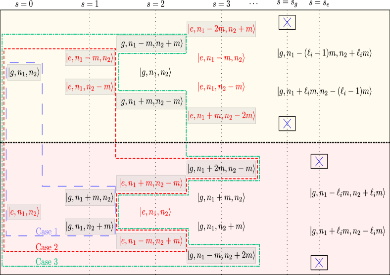
Figure 1: For the tripartite $m$-photon Jaynes-Cummings (MPJC) model ($H$ in Eq.(1)), featuring one qubit initially in a superposition state and two quantized harmonic oscillators occupying arbitrary Fock states $\ket{n_{1}}$ and $\ket{n_{2}}$ respectively, the linear increase in the number of basis states with increasing $n_{1}$ and $n_{2}$ is schematically illustrated. The basis states emerging from $\ket{g,n_{1},n_{2}}$ and $\ket{e,n_{1},n_{2}}$ constitute two complementary sets, as shown in the upper and lower panels. When $H$ acts on $\ket{g,n_{1},n_{2}}$, it generates two new basis states $\ket{e,n_{1}-m,n_{2}}$ and $\ket{e,n_{1},n_{2}-m}$, each contributing one additional basis state. This process results in two distinct arms, where at every second step (denoted by $s=1,\,3,\,5,\cdots$), the number of photons in one of the oscillators is reduced by $m$. The generation of one new basis state at each arm continues until one of the Fock states of that arm is completely annihilated (indicated by blue cross symbols corresponding to $s=s_{g}$ and $s_{e}$). For a fixed $n_{i}$, the total count of new basis states (shown within the rectangular boxes) is $2\ell_{i}-2$, where $\ell_{i}$ is the smallest positive integer for which $n_{i}-\ell_{i}m<0$ ($i=1,\,2$). Similarly, $\ket{e,n_{1},n_{2}}$ gives rise to a total of $2\ell_{i}$ new basis states at each arm. Consequently, the cumulative number of basis states amounts to $4(\ell_{1}+\ell_{2}-1)$. The relevant basis states for the three special cases are respectively depicted within the blue, red, and green dashed regions.

The rest of the article is organized as follows: In the following Section, we introduce the tripartite MPJC model Hamiltonian. In Section III, we analytically explore how a pure initial state of the full system temporally evolves under such a genuinely nonlinear system Hamiltonian. In Section IV, we obtain the reduced states of the oscillators and analyze the efficacy of Fock states swapping between the two oscillators for various cases. In Section V, we investigate the complex dynamics of the Wigner nonclassicalities of various initial oscillator states considering a wide range of system parameters, including the crucial role of various environmentally induced effects. Indicating avenues of further studies, in Section VI, we conclude our article with some brief remarks. Additionally, a set of appendices augmenting the results presented in this work is included at the end.

II The tripartite MPJC Hamiltonian

As mentioned in the previous Section, we are going to analyze a tripartite quantum system comprising one qubit and two oscillators described by the usual free energy Hamiltonian $H_{\text{free}}=\frac{\omega_{0}}{2}\sigma_{z}+\omega_{1}a_{1}^{\dagger}a_{1}+\omega_{2}a_{2}^{\dagger}a_{2},$ where $\sigma_{z}$ is the standard Pauli spin operator and $\omega_{0}$ is the difference in energy between the two levels, $\ket{g}$ and $\ket{e}$ respectively, of the qubit. We use $\hbar=1$ throughout. On the other hand, $a_{1}^{\dagger}$ and $a_{1}$ (similarly, $a_{2}^{\dagger}$ and $a_{2}$) are, respectively, the creation and annihilation operators of the first (second) oscillator with frequency $\omega_{1}$ ($\omega_{2}$).

The qubit simultaneously interacts with both the oscillators through the $m$-photon JC interactions. The interaction Hamiltonian is given by $H_{\text{int}}=\sum_{i=1}^{2}g_{i}\left(a_{i}^{m}\sigma_{+}+a_{i}^{\dagger\,m}\sigma_{-}\right)$, where $\sigma_{+}=\ket{e}\bra{g}$, $\sigma_{-}=\ket{g}\bra{e}$, and the parameter $g_{1}$ ($g_{2}$) determines the strength of the nonlinear MPJC interaction between the qubit and the first (second) oscillator. Further, the integer $m$ tracks the multiphoton process, ($m=1,\,2,\,3,\cdots$). The total Hamiltonian for the tripartite system thus reads

$$H=H_{\text{free}}+H_{\text{int}}.$$ (1)

Following standard convention, we define the two detuning parameters $\Delta_{i}=\omega_{0}-m\omega_{i}$, where $i=1,\,2$. However, throughout this article, we will assume equal frequencies of the two oscillators ($\omega_{1}=\omega_{2}=\omega$) for simplicity. Therefore, $\Delta_{1}=\Delta_{2}=\Delta$. For this simple case, we can split $H=H_{I}+H_{II}$ such that $\left[H,\,H_{II}\right]=0$, where

$$H_{I} =\frac{m\omega}{2}\sigma_{z}+\omega(a_{1}^{\dagger}a_{1}+a_{2}^{\dagger}a_{2}),$$ (2)

$$H_{II} =\frac{\Delta}{2}\sigma_{z}+\sum_{i=1}^{2}g_{i}\left(a_{i}^{m}\sigma_{+}+a_{i}^{\dagger\,m}\sigma_{-}\right).$$ (3)

Now, $H_{I}$ merely introduces a phase contribution in the temporal evolution of the full system. Conveniently, we work with $H_{II}$ and eliminate this trivial time dependence from the dynamics. It is evident that when $m=1$, the system simplifies to the standard tripartite JC model [54]. For a detailed practical implementation of the MPJC Hamiltonian in a specific quantum platform, we refer the reader to Ref. [50].

III Solution: The state vector

Throughout this work, we will assume that the qubit is prepared in a generic superposition state $\cos\phi\ket{g}+\sin\phi\ket{e}$ and the two oscillators are prepared in some arbitrary Fock states $\ket{n_{1}}$ and $\ket{n_{2}}$, respectively. In our notation,

$$\ket{\psi(0)}=\cos\phi\ket{g,n_{1},n_{2}}+\sin\phi\ket{e,n_{1},n_{2}}.$$ (4)

We are interested in the state vector at a later time $\ket{\psi(t)}$ governed by the Hamiltonian $H_{II}$ in Eq.(3), starting with a completely pure initial state $\ket{\psi(0)}$.

In principle, we can obtain the state vector by solving the Schrödinger equation, i.e., $\ket{\psi(t)}=\exp\left(-iH_{II}t\right)\ket{\psi(0)}$. A crucial aspect of this process is understanding how the two basis states $\ket{g,n_{1},n_{2}}$ and $\ket{e,n_{1},n_{2}}$ traverse the JC ladder. This entails determining the precise count of basis states contributing to $\ket{\psi(t)}$ across varying values of $n_{1}$, $n_{2}$, and $m$. While the number of basis states is finite under generic circumstances, determining the exact quantity proves somewhat nontrivial due to the linear increase in required basis states with increasing $n_{1}$, $n_{2}$, and $m$ values, as illustrated schematically in Fig. 1.

Let us begin by examining the initial basis state $\ket{g,n_{1},n_{2}}$ in which the qubit is prepared in the ground state. As depicted in Fig. 1, the application of the MPJC Hamiltonian to $\ket{g,n_{1},n_{2}}$ yields two new states: $\ket{e,n_{1}-m,n_{2}}$ and $\ket{e,n_{1},n_{2}-m}$, respectively. Each of these two new states would subsequently generate another new state. This recursive process of generating new states at each iteration continues until reaching a predetermined finite number of steps, at which point the corresponding Fock states will be annihilated and no further states are produced, thus concluding the JC ladder. By considering the specific values of $n_{i}$, we can identify the smallest positive integer $\ell_{i}$ such that $n_{i}-\ell_{i}m<0$, where $i=1,2$. It is straightforward to see that the state $\ket{n_{i}}$ is annihilated after $2\ell_{i}-1$ steps giving rise to $2\ell_{i}-2$ new basis states. Consequently, the total count of states, including $\ket{g,n_{1},n_{2}}$, is given by $2\ell_{1}-2+2\ell_{2}-2+1=2\ell_{1}+2\ell_{2}-3$.

Similarly, when considering the complementary initial state $\ket{e,n_{1},n_{2}}$ in which the qubit is prepared in the excited state, the calculation proceeds analogously, albeit with a slight modification in the number of steps required for the annihilation of $\ket{n_{i}}$, which is now $2\ell_{i}$, generating $2\ell_{i}-1$ new basis states. Consequently, the total count of states, including $\ket{e,n_{1},n_{2}}$, becomes $2\ell_{1}-1+2\ell_{2}-1+1=2\ell_{1}+2\ell_{2}-1$.

Now, in the most general scenario of initial superposition qubit state $\cos\phi\ket{g}+\sin\phi\ket{e}$, the aggregate number of basis states simply adds up to $2\ell_{1}+2\ell_{2}-3+2\ell_{1}+2\ell_{2}-1=4(\ell_{1}+\ell_{2}-1)$. This is because the basis states for the two marginal cases ($\phi=0$ and $\pi/2$) form two mutually independent sets. Therefore, the $4(\ell_{1}+\ell_{2}-1)$ coupled differential equations obtained from the Schrödinger equation can always be segregated into two sets: one comprising $2\ell_{1}+2\ell_{2}-3$ equations (originating from initial ground qubit state), and the other containing $2\ell_{1}+2\ell_{2}-1$ equations (originating from initial excited qubit state). Further, considering that each basis state can only be connected to a maximum of two new basis states (see Fig. 1), the coupled differential equation governing each time-dependent coefficient will involve, at most, two additional coefficients aside from its own detuning term.

Now, depending upon the specific values of $n_{1}$, $n_{2}$, and $m$, we can identify four different cases. These are: (1) $n_{1},\,n_{2}<m$, (2) $n_{1}<n_{2}=m$ and/or $n_{2}<n_{1}=m$, (3) $n_{1}=n_{2}=m$, and (4) $n_{1},\,n_{2}>m$. For the first three cases, the corresponding $(\ell_{1},\,\ell_{2})$ values are (1, 1), (1, 2) and/or (2, 1), and (2, 2), respectively. In the following, we systematically investigate each of these cases individually.

Case 1: In the constrained scenario where both $n_{1}$ and $n_{2}$ are smaller than $m$, a straightforward observation from Fig. 1 reveals that the state vector at any subsequent time $\ket{\psi(t)}_{1}$ will comprise only four basis states given by

$$\ket{\psi(t)}_{1} =x_{1}(t)\ket{g,n_{1},n_{2}}+y_{1}(t)\ket{e,n_{1},n_{2}}$$

$$+y_{2}(t)\ket{g,n_{1}+m,n_{2}}+y_{3}(t)\ket{g,n_{1},n_{2}+m}.$$ (5)

As explained above, the four coupled differential equations from the Schrödinger equation can be partitioned into two distinct sets: one comprising $2\ell_{1}+2\ell_{2}-3=1$ state, and the other consisting of $2\ell_{1}+2\ell_{2}-1=3$ states (recall that $\ell_{1}=\ell_{2}=1$ in this case) with the initial condition $x_{1}(0)=\cos\phi$, $y_{1}(0)=\sin\phi$, and $y_{3}(0)=y_{4}(0)=0$. The solution to $x(t)$ is trivially obtained to be

$$x_{1}(t) =\cos\phi\,e^{i\Delta^{\prime}t},$$ (6)

where $\Delta^{\prime}=\Delta/2$.

On the other hand, the three coupled differential equations involving the $y$ coefficients can be efficiently expressed as

$$\frac{d}{dt}Y_{1}(t)=-iM_{1_{y}}Y_{1}(t),$$ (7)

where $Y_{1}(t)=\left(y_{1}(t),\,y_{2}(t),\,y_{3}(t)\right)^{\top}$, and the initial condition is $Y_{1}(0)=(\sin\phi,\,0,\,0)^{\top}$. It is straightforward to show that

$$M_{1_{y}}=\begin{pmatrix}\Delta^{\prime}&g_{1_{n_{1}m}}&g_{2_{n_{2}m}}\\ g_{1_{n_{1}m}}&-\Delta^{\prime}&0\\ g_{2_{n_{2}m}}&0&-\Delta^{\prime}\end{pmatrix},$$ (8)

where $g_{1_{n_{1}m}}=\sqrt{(n_{1}+m)!/n_{1}!}\,g_{1}$ and $g_{2_{n_{2}m}}=\sqrt{(n_{2}+m)!/n_{2}!}\,g_{2}$. Now, for the symmetric matrix $M_{1_{y}}$, we can always find an $S$ matrix that diagonalizes $M_{1_{y}}$ such that $M_{1_{y}}=S\,D\,S^{-1}$, with $D$ being the diagonal matrix. The standard solution of Eq.(7) is given by $Y(t)=S\,e^{-iDt}S^{-1}Y(0)$. We have used the Mathematica software and obtained the solutions. The $y$ coefficients after simplifications can be expressed as

$$y_{1}(t) =\sin\phi\left(\cos(\tilde{g}_{1}t)-i\tfrac{\Delta^{\prime}}{\tilde{g}_{1}}\sin\left(\tilde{g}_{1}t\right)\right),$$ (9a)

$$y_{2}(t) =-i\frac{\,g_{1_{n_{1}m}}}{\tilde{g}_{1}}\,\sin\phi\,\sin\left(\tilde{g}_{1}t\right),$$ (9b)

$$y_{3}(t) =-i\frac{g_{2_{n_{2}m}}}{\tilde{g}_{1}}\,\sin\phi\,\sin\left(\tilde{g}_{1}t\right),$$ (9c)

where $\tilde{g}_{1}=\sqrt{g_{1_{n_{1}m}}^{2}+g_{2_{n_{2}m}}^{2}+\Delta^{\prime 2}}$.

Case 2: Next, we consider the case $n_{1}<n_{2}=m$. This corresponds to $\ell_{1}=1$, $\ell_{2}=2$. Consequently, the state vector $\ket{\psi(t)}_{2}$ in this case will be a superposition of a total of eight basis states given by

$$\ket{\psi(t)}_{2} =x_{1}(t)\ket{g,n_{1},m}+x_{2}(t)\ket{e,n_{1},0}$$

$$+x_{3}(t)\ket{g,n_{1}+m,0}+y_{1}(t)\ket{e,n_{1},m}$$

$$+y_{2}(t)\ket{g,n_{1}+m,m}+y_{3}(t)\ket{g,n_{1},2m},$$

$$+y_{4}(t)\ket{e,n_{1}+m,0}+y_{5}(t)\ket{g,n_{1}+2m,0}.$$ (10)

Now, addressing the coupled differential equations involving the $x$ and $y$ coefficients independently, the two sets of equations can be expressed compactly (similar to Eq.(7)) as

$$\frac{d}{dt}X_{2}(t)=-iM_{2_{x}}X_{2}(t),\quad\frac{d}{dt}Y_{2}(t)=-iM_{2_{y}}Y_{2}(t),$$ (11)

where $X_{2}(t)=\left(x_{1}(t),\,x_{2}(t),\,x_{3}(t)\right)^{\top}$, and $Y_{2}(t)=\left(y_{1}(t),\,y_{2}(t),\,y_{3}(t),\,y_{4}(t),\,y_{5}(t)\right)^{\top}$. The initial conditions are given by $X_{2}(0)=(\cos\phi,\,0,\,0)^{\top}$, $Y_{2}(0)=(\sin\phi,\,0,\,0,\,0,\,0)^{\top}$. The exact forms of the two symmetric matrices $M_{2_{x}}$ and $M_{2_{y}}$ can be found in Appendix A. As before, we have utilized the Mathematica software to obtain the solution. After simplification, the $x$ coefficients read as

$$x_{1}(t) =f_{1}\left(\cos\left(\tilde{g}_{2}t\right)+i\tfrac{\Delta^{\prime}}{\tilde{g}_{2}}\sin\left(\tilde{g}_{2}t\right)+f_{0}\,e^{i\Delta^{\prime}t}\right),$$ (12a)

$$x_{2}(t) =-if_{2}\sin\left(\tilde{g}_{2}t\right),$$ (12b)

$$x_{3}(t) =f_{3}\left(\cos\left(\tilde{g}_{2}t\right)+i\tfrac{\Delta^{\prime}}{\tilde{g}_{2}}\sin\left(\tilde{g}_{2}t\right)-e^{i\Delta^{\prime}t}\right),$$ (12c)

where $\tilde{g}_{2}=\sqrt{g_{1_{n_{1}m}}^{2}+g_{2_{m}}^{2}+\Delta^{\prime 2}}$ , $g_{2_{m}}=\sqrt{m!}\,g_{2}$, $f_{0}=\tfrac{g_{1_{n_{1}m}}^{2}}{g_{2_{m}}^{2}}$, $f_{1}=\frac{g_{2_{m}}^{2}}{g_{1_{n_{1}m}}^{2}+g_{2_{m}}^{2}}\cos\phi$, $f_{2}=\frac{g_{2_{m}}}{\tilde{g}_{2}}\cos\phi$, and $f_{3}=\frac{g_{1_{n_{1}m}}g_{2_{m}}}{g_{1_{n_{1}m}}^{2}+g_{2_{m}}^{2}}\cos\phi$.

On the other hand, expressing the $y$ coefficients in simple algebraic forms appears challenging in the most general situation. However, ignoring the detuning (that is, setting $\Delta=0$ or considering only $H_{\text{int}}$), it is possible to express these coefficients succinctly. After simplifications, we obtain

$$y_{1}(t) =\tfrac{\sin\phi}{s}\left(\tilde{\textsl{g}}_{s_{+}}^{\prime 2}\cos\tau_{+}-\tilde{\textsl{g}}_{s_{-}}^{\prime 2}\cos\tau_{-}\right),$$ (13a)

$$y_{2}(t) =-i\tfrac{\sin\phi}{s}\left(f_{2_{+}}\sin\tau_{+}-f_{2_{-}}\sin\tau_{-}\right),$$ (13b)

$$y_{3}(t) =i\tfrac{\sin\phi}{s}\left(f_{3_{+}}\sin\tau_{+}-f_{3_{-}}\sin\tau_{-}\right),$$ (13c)

$$y_{4}(t) =\tfrac{\sin\phi}{s}\textsl{g}_{1}\textsl{g}_{3}\left(\cos\tau_{+}-\cos\tau_{-}\right),$$ (13d)

$$y_{5}(t) =-i\tfrac{\sin\phi}{s}\textsl{g}_{1}\textsl{g}_{3}\textsl{g}_{4}\left(\tfrac{\sin\tau_{+}}{\tilde{\textsl{g}}_{s_{+}}}-\tfrac{\sin\tau_{-}}{\tilde{\textsl{g}}_{s_{-}}}\right).$$ (13e)

Here, $s=\sqrt{G^{4}-4\mathcal{G}^{4}}$, $\tilde{\textsl{g}}_{s_{\pm}}=\sqrt{\tfrac{1}{2}\left(G^{2}\pm s\right)}$, $\tilde{\textsl{g}}_{s_{\pm}}^{\prime 2}=\tfrac{1}{2}\left(G^{\prime 2}\pm s\right)$, $G^{2}=\textsl{g}_{1}^{2}+\textsl{g}_{2}^{2}+\textsl{g}_{3}^{2}+\textsl{g}_{4}^{2}$, $G^{\prime 2}=\textsl{g}_{1}^{2}+\textsl{g}_{2}^{2}-\textsl{g}_{3}^{2}-\textsl{g}_{4}^{2}$, $\mathcal{G}^{4}=\left(\textsl{g}_{1}^{2}\textsl{g}_{4}^{2}+\textsl{g}_{2}^{2}\textsl{g}_{3}^{2}+\textsl{g}_{2}^{2}\textsl{g}_{4}^{2}\right)$, $f_{2\pm}=\textsl{g}_{1}\tilde{\textsl{g}}_{s_{\pm}}\left(\textsl{g}_{2}^{2}\textsl{g}_{3}^{2}+\textsl{g}_{4}^{2}\tilde{\textsl{g}}_{s_{\pm}}^{\prime 2}\right)/\mathcal{G}^{4}$, $f_{3_{+}}=\textsl{g}_{2}\tilde{\textsl{g}}_{s_{+}}\left(\textsl{g}_{1}^{2}\textsl{g}_{3}^{2}-\left(\textsl{g}_{3}^{2}+\textsl{g}_{4}^{2}\right)\tilde{\textsl{g}}_{s_{+}}^{\prime 2}\right)/\mathcal{G}^{4}$, $f_{3_{-}}=\textsl{g}_{2}\tilde{\textsl{g}}_{s_{-}}\left(\textsl{g}_{1}^{2}\textsl{g}_{4}^{2}-\left(\textsl{g}_{3}^{2}+\textsl{g}_{4}^{2}\right)\tilde{\textsl{g}}_{s_{-}}^{\prime 2}\right)/\mathcal{G}^{4}$, and $\tau_{\pm}=\tilde{\textsl{g}}_{s_{\pm}}t$. Further, $\textsl{g}_{1}=\sqrt{(n_{1}+m)!/n_{1}!}\,g_{1}$, $\textsl{g}_{2}=\sqrt{(2m)!/m!}\,g_{2}$, $\textsl{g}_{3}=\sqrt{(n_{1}+2m)!/(n_{1}+m)!}\,g_{1}$, and $\textsl{g}_{4}=\sqrt{m!}\,g_{2}$.

Before progressing to the subsequent scenario, we note that the case where $n_{2}<n_{1}=m$, corresponding to $\ell_{1}=2$ and $\ell_{1}=1$, is complementary to the situation where $n_{1}<n_{2}=m$.

Case 3: Now, let us examine the scenario where $n_{1}=n_{2}=m$, corresponding to $\ell_{1}=\ell_{2}=2$. In this special case, the state vector comprises twelve basis states (partitioned into two sets consisting of five and seven states respectively) and is given by

$$\ket{\psi(t)}_{3} =x_{1}\ket{g,m,m}+x_{2}\ket{e,0,m}+x_{3}\ket{e,m,0}$$

$$\,\,\,+x_{4}\ket{g,2m,0}+x_{5}\ket{g,0,2m}+y_{1}\ket{e,m,m}$$

$$\,\,\,+y_{2}\ket{g,2m,m}+y_{3}\ket{g,m,2m}+y_{4}\ket{e,2m,0}$$

$$\,\,\,+y_{5}\ket{e,0,2m}+y_{6}\ket{g,3m,0}+y_{7}\ket{g,0,3m}.$$ (14)

Note that for brevity, we ignore the explicit time dependencies of the coefficients $x$ and $y$ in Eq.(14). Analogous to Eq.(11), we can express the coupled differential equations involving the coefficients $x$ and $y$ as

$$\frac{d}{dt}X_{3}(t)=-iM_{3_{x}}X_{3}(t),\quad\frac{d}{dt}Y_{3}(t)=-iM_{3_{y}}Y_{3}(t).$$ (15)

Here, $X_{3}(t)=\left(x_{1}(t),\,x_{2}(t),\,x_{3}(t),\,x_{4}(t),\,x_{5}(t)\right)^{\top}$, and $Y_{2}(t)=\left(y_{1}(t),\,y_{2}(t),\,y_{3}(t),\,y_{4}(t),\,y_{5}(t),\,y_{6}(t),\,y_{7}(t)\right)^{\top}$. The initial conditions are given by $X_{2}(0)=(\cos\phi,\,0,\,0,\,0,\,0)^{\top}$, $Y_{2}(0)=(\sin\phi,\,0,\,0,\,0,\,0,\,0,\,0)^{\top}$. The elements of the symmetric matrices $M_{3_{x}}$ and $M_{3_{y}}$ are detailed in Appendix A. Analogously to the $y$ coefficients for case 2, we can express the solution for the $x$ coefficients in compact algebraic forms in the limit $\Delta=0$. Following a few simplification steps, we obtain

$$x_{1}(t) =\tfrac{\cos\phi}{f_{0}}\left(f_{1_{+}}\cos\tau_{+}-f_{1_{-}}\cos\tau_{-}-s\textsl{g}_{3}^{2}\textsl{g}_{4}^{2}\right),$$ (16a)

$$x_{2}(t) =-i\tfrac{\cos\phi}{f_{0}}\left(f_{2_{+}}\sin\tau_{+}-f_{2_{-}}\sin\tau_{-}\right),$$ (16b)

$$x_{3}(t) =-i\tfrac{\cos\phi}{f_{0}}\left(f_{3_{+}}\sin\tau_{+}-f_{3_{-}}\sin\tau_{-}\right),$$ (16c)

$$x_{4}(t) =\tfrac{\cos\phi}{f_{0}}\left(f_{4_{+}}\cos\tau_{+}-f_{4_{-}}\cos\tau_{-}-s\textsl{g}_{1}\textsl{g}_{3}^{2}\textsl{g}_{4}\right),$$ (16d)

$$x_{5}(t) =\tfrac{\cos\phi}{f_{0}}\left(f_{5_{+}}\cos\tau_{+}-f_{5_{-}}\cos\tau_{-}-s\textsl{g}_{2}\textsl{g}_{3}\textsl{g}_{4}^{2}\right).$$ (16e)

Here, $s=\sqrt{G^{4}-4\left(\textsl{g}_{1}^{2}\textsl{g}_{3}^{2}+\textsl{g}_{2}^{2}\textsl{g}_{4}^{2}+\textsl{g}_{3}^{2}\textsl{g}_{4}^{2}\right)}$, $\tilde{\textsl{g}}_{s_{\pm}}=\sqrt{\tfrac{1}{2}\left(G^{2}\pm s\right)}$, $\tilde{\textsl{g}}_{s_{\pm}}^{\prime}=\sqrt{\tfrac{1}{2}\left(G^{\prime 2}\pm s\right)}$, $G^{2}=\textsl{g}_{1}^{2}+\textsl{g}_{2}^{2}+\textsl{g}_{3}^{2}+\textsl{g}_{4}^{2}$, $G^{\prime 2}=\textsl{g}_{1}^{2}-\textsl{g}_{2}^{2}-\textsl{g}_{3}^{2}+\textsl{g}_{4}^{2}$. Further, $f_{0}=s\tilde{\textsl{g}}_{s_{+}}^{2}\tilde{\textsl{g}}_{s_{-}}^{2}$, $f_{1_{\pm}}=\textsl{g}_{1}^{2}\textsl{g}_{3}^{4}+\textsl{g}_{2}^{2}\textsl{g}_{4}^{4}-\left(\textsl{g}_{1}^{2}\textsl{g}_{3}^{2}+\textsl{g}_{2}^{2}\textsl{g}_{4}^{2}\right)\tilde{\textsl{g}}_{s_{\pm}}^{2}$, $f_{2_{\pm}}=\textsl{g}_{1}\left(\textsl{g}_{2}^{2}\textsl{g}_{4}^{2}+\textsl{g}_{3}^{2}\tilde{\textsl{g}}_{s_{\pm}}^{\prime 2}\right)\tilde{\textsl{g}}_{s_{\pm}}$, $f_{3_{\pm}}=\textsl{g}_{2}\left(\textsl{g}_{1}^{2}\textsl{g}_{3}^{2}-\textsl{g}_{4}^{2}\tilde{\textsl{g}}_{s_{\mp}}^{\prime 2}\right)\tilde{\textsl{g}}_{s_{\pm}}$, $f_{4_{\pm}}=\textsl{g}_{1}\textsl{g}_{4}\left(\textsl{g}_{2}^{2}\textsl{g}_{4}^{2}+\textsl{g}_{3}^{2}\tilde{\textsl{g}}_{s_{\pm}}^{\prime 2}\right)$, $f_{5_{\pm}}=\textsl{g}_{2}\textsl{g}_{3}\left(\textsl{g}_{1}^{2}\textsl{g}_{3}^{2}-\textsl{g}_{4}^{2}\tilde{\textsl{g}}_{s_{\mp}}^{\prime 2}\right)$, and $\tau_{\pm}=\tilde{\textsl{g}}_{s_{\pm}}t$. Finally, $\textsl{g}_{1}=\sqrt{m!}\,g_{1}$, $\textsl{g}_{2}=\sqrt{m!}\,g_{2}$, $\textsl{g}_{3}=\sqrt{(2m)!/m!}\,g_{1}$, and $\textsl{g}_{4}=\sqrt{(2m)!/m!}\,g_{2}$.

On the other hand, despite setting $\Delta=0$, it remains challenging to express the seven $y$ coefficients in simple algebraic terms, even with the assistance of the Mathematica software.

Case 4: In the final case, where both $n_{1}$ and $n_{2}$ exceed $m$, the state vector at a later time, $\ket{\psi(t)}_{4}$, can be realized by following the JC ladder, as depicted in Fig. 1. We employ a similar methodology for arbitrary values of $n_{1}$, $n_{2}$ and $m$, and construct two independent state vectors $\ket{\psi_{x}(t)}_{4}$ and $\ket{\psi_{y}(t)}_{4}$ (or equivalently $X_{4}(t)$ and $Y_{4}(t)$), such that $\ket{\psi(t)}_{4}=\ket{\psi_{x}(t)}_{4}+\ket{\psi_{y}(t)}_{4}$. The exact forms of $\ket{\psi_{x}(t)}_{4}$ and $\ket{\psi_{y}(t)}_{4}$ are provided in Appendix A. Following the Schrödinger equation, we can derive the corresponding coupled differential equations of $X_{4}(t)$ and $Y_{4}(t)$, akin to Eqs.(11) and (15). This leads to the determination of two symmetric square matrices, denoted as $M_{4_{x}}$ and $M_{4_{y}}$, whose generic forms can be found in Appendix A. Both $M_{x}$ and $M_{y}$ exhibit a pentadiagonal structure and are, in principle, diagonalizable. Nevertheless, expressing the two generic state vectors $X_{4}(t)$ and $Y_{4}(t)$ in simple algebraic forms remains a formidable task.

IV Time-evolved oscillator states

In this Section, we will extract the time-evolved states of each oscillator by tracing over the relevant subsystems from the corresponding state vectors for all cases. Additionally, we will assess the effectiveness of swapping Fock states between the two oscillators for all scenarios. Recall that the two oscillators are initially in arbitrary Fock states $\ket{n_{1}}$ and $\ket{n_{2}}$ respectively, with the joint oscillator state expressed as $\ket{n_{1},\,n_{2}}$. Perfect state swapping therefore entails transforming $\ket{n_{1},\,n_{2}}$ into $\ket{n_{2},\,n_{1}}$. For simplicity, we assume $\Delta=0$ and $g_{1}=g_{2}=g$ for the analysis.

Case 1: Obtaining the reduced density matrices of the two oscillators $\rho_{1}^{(1)}(t)$ and $\rho_{2}^{(1)}(t)$ from $\ket{\psi(t)}_{1}$ in Eq.(5) is straightforward. Since only two basis states for each oscillator ($\ket{n_{i}}$ and $\ket{n_{i}+m}$ respectively, where $i=1,\,2$) are involved in the dynamics, the reduced density matrices can be effectively represented as $2\times 2$ matrices and are given by

$$\rho_{1}^{(1)}(t)=\begin{pmatrix}1-|y_{2}|^{2}&x_{1}y_{2}^{*}\\ x_{1}^{*}y_{2}&|y_{2}|^{2}\end{pmatrix},$$ (17)

and

$$\rho_{2}^{(1)}(t)=\begin{pmatrix}1-|y_{3}|^{2}&x_{1}y_{3}^{*}\\ x_{1}^{*}y_{3}&|y_{3}|^{2}\end{pmatrix},$$ (18)

respectively. The $x$ and $y$ coefficients are given by Eqs.(6) and (9), respectively. Now, with $\Delta=0$ and $g_{1}=g_{2}=g$, we have $\tilde{g}_{1}=\sqrt{g_{1_{n_{1}m}}^{2}+g_{2_{n_{2}m}}^{2}}$, where $g_{n_{i}m}=\sqrt{\frac{(n_{i}+m)!}{n_{i}!}}g$. Therefore, $\frac{g_{1_{n_{1}m}}}{\tilde{g}_{1}}=\left(1+\frac{n_{1}!}{n_{2}!}\right)^{-1/2}$, and $\frac{g_{2_{n_{2}m}}}{\tilde{g}_{1}}=\left(1+\frac{n_{2}!}{n_{1}!}\right)^{-1/2}$. Now, it is evident that if the qubit starts from the ground state ($\phi=0$), only the $x_{1}$ coefficient survives. Consequently, the state vector $\ket{\psi(t)}_{1}$ and thus both the oscillator Fock states acquire only an overall phase during the dynamics, implying $\ket{n_{1},\,n_{2}}\longrightarrow e^{i\theta}\ket{n_{1},\,n_{2}}$.

On the other hand, if the qubit is initially prepared in the excited state ($\phi=\pi/2$), then $x_{1}=0$. Therefore, the off-diagonal elements of both $\rho_{1}^{(1)}$ and $\rho_{1}^{(2)}$ become zero. Consequently, the time-evolved oscillator states transform into a trivial incoherent mixture of the two basis states $\ket{n_{i}}$ and $\ket{n_{i}+m}$, that is, $\rho_{1}^{(1)}=\text{diag}\left(1-|y_{2}|^{2},\,|y_{2}|^{2}\right)$ and $\rho_{2}^{(1)}=\text{diag}\left(1-|y_{3}|^{2},\,|y_{3}|^{2}\right)$.

Now, it is obvious from Eq.(5) that whenever $|y_{2}|^{2}=1$ or $|y_{3}|^{2}=1$ the joint oscillator state becomes $\ket{n_{1}+m,\,n_{2}}$ or $\ket{n_{1},\,n_{2}+m}$. However, $|y_{2}|^{2}$ or $|y_{3}|^{2}$ oscillates between zero and $\left(1+\frac{n_{1}!}{n_{2}!}\right)^{-1}$ or zero and $\left(1+\frac{n_{2}!}{n_{1}!}\right)^{-1}$ in this case. Therefore, $|y_{2}|^{2}\to 1$ (or $|y_{2}|^{2}\to 1$) in the limit $n_{2}\to\infty$ (or $n_{1}\to\infty$) which is not feasible for this case, as both $n_{1},\,n_{2}<m$. Finally, we note in passing that for other values of $\phi$, the two oscillator states remain a superposition state of the two effective basis states.

Case 2: Unlike the previous scenario, in this case, three basis states for each oscillator ($\ket{n_{1}}$, $\ket{n_{1}+m}$, and $\ket{n_{1}+2m}$ for the first oscillator and $\ket{0}$, $\ket{m}$, and $\ket{2m}$ for the second oscillator, respectively) are involved in the dynamics. Therefore, the reduced density matrices of both the oscillators $\rho_{1}^{(2)}(t)$ and $\rho_{2}^{(2)}(t)$ can be effectively expressed as $3\times 3$ matrices. These are given by

$$\rho_{1}^{(2)}(t) =\begin{pmatrix}|x_{1}|^{2}+|x_{2}|^{2}+|y_{1}|^{2}+|y_{3}|^{2}&x_{1}y_{2}^{*}+x_{2}y_{4}^{*}&0\\ y_{2}x_{1}^{*}+y_{4}x_{2}^{*}&|x_{3}|^{2}+|y_{2}|^{2}+|y_{4}|^{2}&x_{3}y_{5}^{*}\\ 0&y_{5}x_{3}^{*}&|y_{5}|^{2}\end{pmatrix},$$ (19)

and

$$\rho_{2}^{(2)}(t) =\begin{pmatrix}|x_{2}|^{2}+|x_{3}|^{2}+|y_{4}|^{2}+|y_{5}|^{2}&x_{2}y_{1}^{*}+x_{3}y_{2}^{*}&0\\ y_{1}x_{2}^{*}+y_{2}x_{3}^{*}&|x_{1}|^{2}+|y_{1}|^{2}+|y_{2}|^{2}&x_{1}y_{3}^{*}\\ 0&y_{3}x_{1}^{*}&|y_{3}|^{2}\end{pmatrix},$$ (20)

respectively. Once again, for $\phi=0$, (initial ground state qubit), only the $x$ coefficients contribute. Consequently, the first oscillator becomes an incoherent mixture of only two basis states: $\ket{n_{1}}$ and $\ket{n_{1}+m}$. That is, $\rho_{1}^{(2)}=\text{diag}\left(1-|x_{3}|^{2},\,|x_{3}|^{2}\right)$. Similarly, the second oscillator state becomes an incoherent mixture of $\ket{0}$ and $\ket{m}$, leading to $\rho_{2}^{(2)}=\text{diag}\left(1-|x_{1}|^{2},\,|x_{1}|^{2}\right)$. It is easy to see that for $\Delta=0$ and $g_{1}=g_{2}=g$, we have

$$|x_{1}| =\frac{(n_{1}!+m!)+n_{1}!m!\cos\left(\tilde{g}t\right)}{n_{1}!m!+(n_{1}+m)!},$$ (21)

$$|x_{3}| =2\frac{\sqrt{n_{1}!m!(n_{1}+m)!}}{n_{1}!m!+(n_{1}+m)!}\sin^{2}\left(\tfrac{1}{2}\tilde{g}t\right),$$ (22)

where $\tilde{g}=\sqrt{\frac{(n_{1}+m)!+n_{1}!m!}{n_{1}!}}g$. It is evident that for $n_{1}=0$, we obtain $|x_{1}|=\cos^{2}\left(\sqrt{\tfrac{m!}{2}}gt\right)$ and $|x_{3}|=\sin^{2}\left(\sqrt{\tfrac{m!}{2}}gt\right)$. In contrast to the previous scenario, both $|x_{1}|$ and $|x_{3}|$ can attain the highest value of unity if we assume $n_{1}=0$. When $|x_{3}|=1$, all excitations of the second oscillator are transferred to the first oscillator, resulting in a perfect swapping of Fock states between the oscillators, i.e., $\ket{0,\,m}\longrightarrow\ket{m,\,0}$. It is noteworthy that with standard Jaynes-Cummings couplings, only the swapping of the first excited state with the ground state is achievable. However, we find that with MPJC interactions, swapping of arbitrary Fock states can be achieved, in principle. Conversely, since $|x_{3}|$ cannot reach the value of 1, for $n_{1}>0$, all excitations of the second oscillator cannot be transferred to the first oscillator; thus, $\ket{n_{1},\,m}\longrightarrow\ket{n_{1}+m,\,0}$ is not feasible with unit fidelity if $n_{1}>0$.

Now, suppose the qubit is initially prepared in the excited state (i.e., $\phi=\pi/2$). In this scenario, all $x$ coefficients vanish, resulting in $\rho_{1}^{(2)}$ and $\rho_{2}^{(2)}$ being strictly diagonal, comprising all three basis states in each case. That is, $\rho_{1}^{(2)}=\text{diag}\left(|y_{1}|^{2}+|y_{3}|^{2},\,|y_{2}|^{2}+|y_{4}|^{2},\,|y_{5}|^{2}\right)$, and $\rho_{2}^{(2)}=\text{diag}\left(|y_{4}|^{2}+|y_{5}|^{2},\,|y_{1}|^{2}+|y_{2}|^{2},\,|y_{3}|^{2}\right)$. Unlike all the previous subcases, here we find that the dynamics is controlled by two different frequencies $\tilde{\textsl{g}}_{s_{\pm}}$ (see Eq.(13)). In the simplest case, when $n_{1}=0$ (along with $\Delta=0$, $g_{1}=g_{2}=g$), we obtain

$$y_{4} =\frac{1}{\sqrt{2(2m)!}}\left(\cos(\tilde{\textsl{g}}_{s_{+}}t)-\cos(\tilde{\textsl{g}}_{s_{-}}t)\right),$$ (23a)

$$y_{5} =-i\tfrac{\sqrt{m!}}{2}\left(\frac{\sin(\tilde{\textsl{g}}_{s_{+}}t)}{\tilde{\textsl{g}}_{s_{+}}}-\frac{\sin(\tilde{\textsl{g}}_{s_{-}}t)}{\tilde{\textsl{g}}_{s_{-}}}\right),$$ (23b)

where $\tilde{\textsl{g}}_{s_{\pm}}=\sqrt{m!+(2m)!/m!\pm\sqrt{(2m)!}}\,g$. It can be shown that $|y_{4}|$ or $|y_{5}|$ can never reach the value of unity. Therefore, we can conclude that $\ket{0,\,m}\longrightarrow\ket{m,\,0}$ or $\ket{0,\,m}\longrightarrow\ket{2m,\,0}$ is also not feasible in this case. For higher values of $n_{1}$, the analysis becomes even more intricate. However, we can see that the two oscillator states remain an incoherent mixture of the three corresponding basis states.

Case 3: For this case, the reduced density matrices for the two oscillators can be effectively expressed in the $\ket{0}$, $\ket{m}$, $\ket{2m}$, and $\ket{3m}$ basis. The exact analytical expressions of $\rho_{1}^{(3)}(t)$ and $\rho_{2}^{(3)}(t)$ can be found in Appendix A. Specifically, for $\phi=0$ (for which we could obtain an exact analytical solution, assuming $\Delta=0$), the two oscillator states reduce to an incoherent mixture of the three basis states $\ket{0}$, $\ket{m}$, and $\ket{2m}$. These are given by $\rho_{1}^{(3)}=\text{diag}\left(|x_{2}|^{2}+|x_{5}|^{2},|x_{1}|^{2}+|x_{3}|^{2},|x_{4}|^{2}\right)$ and $\rho_{2}^{(3)}=\text{diag}\left(|x_{3}|^{2}+|x_{4}|^{2},|x_{1}|^{2}+|x_{2}|^{2},|x_{5}|^{2}\right)$, respectively. The feasibility of $\ket{m,\,m}\longrightarrow\ket{2m,\,0}$ or $\ket{m,\,m}\longrightarrow\ket{0,\,2m}$ can be obtained by calculating $|x_{4}|$ and $|x_{5}|$ in Eq.(16). Now, even for the simplest case with $m=1$, it can be shown (assuming $g_{1}=g_{2}=g$) that $|x_{1}|^{2}$ oscillates between 0 and 1, $|x_{2}|^{2}$ and $|x_{3}|^{2}$ between 0 and $\frac{1}{4}$, and $|x_{4}|^{2}$ and $|x_{5}|^{2}$ between 0 and $\frac{1}{2}$. In particular, $|x_{4}|=|x_{5}|=\tfrac{1}{\sqrt{2}}\sin^{2}(\sqrt{2}gt)$, clearly indicating that even $\ket{1,\,1}\longrightarrow\ket{2,\,0}$ or $\ket{1,\,1}\longrightarrow\ket{0,\,2}$ is not feasible in this case. However, the fact that $|x_{1}|^{2}=1$ at periodic intervals, $\ket{1}$ returns to itself periodically. In fact, it can be easily shown that $|x_{1}|^{2}=1$ for all values of $m$, indicating the periodic return of $\ket{m}$ during the temporal evolution. However, the amplitude of the oscillations for other $x$ coefficients depends on the specific choice of the parameter $m$. For completeness, we note that for $\phi=\pi/2$, the two oscillator states are $\rho_{1}^{(3)}=\text{diag}\left(|y_{5}|^{2}+|y_{7}|^{2},|y_{1}|^{2}+|y_{3}|^{2},|y_{2}|^{2}+|y_{4}|^{2},|y_{6}|^{2}\right)$ and $\rho_{2}^{(3)}=\text{diag}\left(|y_{4}|^{2}+|y_{6}|^{2},|y_{1}|^{2}+|y_{2}|^{2},|y_{3}|^{2}+|y_{5}|^{2},|y_{7}|^{2}\right)$ in the $\ket{0}$, $\ket{m}$, $\ket{2m}$, and $\ket{3m}$ basis.

Case 4: Lastly, for this case as well, we can derive general expressions for the reduced density matrices of the two oscillators $\rho_{1}^{(4)}$ and $\rho_{2}^{(4)}$ using a similar methodology (see Appendix A for details). Similar to previous cases, we found both matrices to be tridiagonal. Nevertheless, drawing general conclusions without knowledge of specific values for $n_{1}$, $n_{2}$, and $m$ remains challenging.

V Wigner nonclassicalities

As noted in Section I, Fock states exhibit pronounced nonclassical behavior. A commonly employed method to quantify the extent of nonclassicality in a given quantum state involves computing the volume of the negative region within its associated Wigner function, defined as [51, 52, 53]

$$V_{W_{-}}=-\iint dx\,dp\,\min\left[W(x,p),0\right],$$ (24)

where the integration encompasses the entire phase space and $\iint dx\,dp\,W(x,p)=1$ is the normalization condition. As per definition, $V_{W_{-}}$ equals zero for all Gaussian states, including the vacuum $\ket{0}$, coherent state $\ket{\alpha}$, or squeezed vacuum state $\ket{\xi}$.

A natural question arises: how does this measure of nonclassicality evolve under such a nonlinear Hamiltonian? We address this question in the following, assuming the initial state of the tripartite system is $\ket{\psi(0)}$ in Eq.(4), that is the qubit is in superposition state and the two oscillators are in arbitrary Fock states $\ket{n_{1}}$ and $\ket{n_{2}}$ respectively. For brevity, we discuss here only the evolution of $V_{W_{1-}}$ of the first oscillator Fock state $\ket{n_{1}}$, as similar results can also be obtained for the second oscillator.

To simplify the analysis, we set $g_{1}=g_{2}=1/\sqrt{2}$ and $\Delta=0$ (see, however, Appendix B where the role of detuning is analyzed in detail), while restricting ourselves to $n_{1},\,n_{2},\,m\leqslant 3$. Additionally, we mainly consider three specific values for $\phi$: $0$, $\pi/4$, and $\pi/2$, corresponding to ground, maximally superposed, and excited initial qubit states, respectively. It is worth mentioning that the Wigner function of the photon number state $\ket{n}$ is given by $W(\alpha)=\frac{2}{\pi}(-1)^{n}e^{-2|\alpha|^{2}}L_{n}\left(4|\alpha|^{2}\right)$, where $\alpha=(x+ip)/\sqrt{2}$ and $L_{n}(\,\cdot\,)$ is the standard Laguerre polynomial (see Appendix C).

Figure 2: For the tripartite $m$-photon Jaynes-Cummings (MPJC) model, described by the Hamiltonian $H$ in Eq.(1), the temporal evolution of the Wigner nonclassicality (quantified by the volume of the negative region of the associated Wigner function $V_{W_{1-}}$ in Eq.(24)) of the initial Fock states $\ket{0}$, $\ket{1}$, and $\ket{2}$ (as represented by the blue, the black, and the red curves, respectively) of the first oscillator is illustrated for case 1 (that is when $n_{1},\,n_{2}<m$). Initially, the second oscillator is in the vacuum state $\ket{0}$ and the qubit is initially in a superposition state with (a) $\phi=\pi/4$ and (b) $\phi=\pi/2$. Further, $m=3$, and we set $g_{1}=g_{2}=1/\sqrt{2}$ and $\Delta=0$. In both panels, $V_{W_{1-}}$ surpasses its initial value (denoted by dashed horizontal lines) by significant amounts. More importantly, driven by the initial qubit energy alone, with both the oscillators initialized in the ground states, the MPJC interactions nontrivially produce negativity in the Wigner functions in both cases.

Case 1: We begin by examining case 1 ($n_{1},\,n_{2}<m$). The time-evolved Wigner function of the first oscillator is found to be (see Appendix C for details)

$$\tilde{W}_{1}(\alpha,t) =(-1)^{n_{1}}\Big{[}\left(1-|y_{2}|^{2}\right)L_{n_{1}}(z)+2^{m}\sqrt{\tfrac{n_{1}!}{(n_{1}+m)!}}$$

$$\hskip 54.2025pt\times\big{(}x_{1}y_{2}^{*}\alpha^{m}+y_{2}x_{1}^{*}(\alpha^{*})^{m}\big{)}L_{n_{1}}^{m}(z)$$

$$\hskip 61.42993pt+(-1)^{m}|y_{2}|^{2}L_{n_{1}+m}(z)\Big{]},$$ (25)

where $W_{1}(\alpha,t)=\frac{2}{\pi}e^{-2|\alpha|^{2}}\tilde{W}_{1}(\alpha,t)$, $z=4|\alpha|^{2}$, and $L_{k_{1}}^{k_{2}}(\,\cdot\,)$ is the associated Laguerre polynomial. For clarity, we consistently employ this notation in the equations for the Wigner functions through the remainder of this paper. The time-dependent coefficients $x$ and $y$ are given by Eq.(9). As already discussed in the preceding Sections, the system undergoes trivial temporal evolution for $\phi=0$. Notably, the $y$ coefficients become zero, and $|x_{1}|=1$. It is straightforward to see that $W_{1}(\alpha,t)=\frac{2}{\pi}(-1)^{n_{1}}e^{-2|\alpha|^{2}}L_{n_{1}}\left(4|\alpha|^{2}\right)=W_{1}(\alpha,0)$ in this case. Thus, $V_{W_{1-}}$ remains constant over time.

However, the evolution becomes nontrivial for other values of $\phi$, as the $y$ coefficients now contribute to the dynamics. Depending on the specific values of $n_{1}$, $n_{2}$, and $m$, significant changes manifest in the dynamics of $V_{W_{1-}}$, as illustrated in Fig. 2. For example, consider the simplest case where the system is driven solely by the initial qubit energy, that is, both oscillators are initialized in the ground states characterized by Gaussian Wigner functions with no negative regions. Setting $n_{1}=n_{2}=0$ in Eq.(25), the Wigner function of the first oscillator becomes

$$\tilde{W}_{1}(\alpha,t) =1-|y_{2}|^{2}\left(1-(-1)^{m}L_{m}(z)\right)$$

$$\quad\quad+\frac{2^{m}}{\sqrt{m!}}\left(x_{1}y_{2}^{*}\alpha^{m}+x_{1}^{*}y_{2}(\alpha^{*})^{m}\right).$$ (26)

For the standard JC interactions ($m=1$), the above expression further simplifies to (using $L_{1}(z)=1-z$)

$$\tilde{W}_{1}(\alpha,t)=1-2\left(1-2|\alpha|^{2}\right)|y_{2}|^{2}+4\text{Re}(x_{1}y_{2}^{*}\alpha).$$ (27)

Now, using $g_{1}=g_{2}=1/\sqrt{2}$ and $\Delta=0$, we get $x_{1}=\cos\phi$, $y_{2}=-\frac{i}{\sqrt{2}}\sin\phi\sin(t)$. Substituting these in Eq.(27), we obtain

$$\tilde{W}_{1}(\alpha,t) =\sin^{2}\phi\cos^{2}t+\cos^{2}\phi\cos^{2}\theta$$

$$+\left(\sqrt{2}|\alpha|\sin\phi\sin t-\cos\phi\sin\theta\right)^{2},$$ (28)

where we have used $\alpha=|\alpha|e^{i\theta}$. Evidently, $W_{1}(\alpha,t)$ is always positive resulting in $V_{W_{1-}}=0$ for all times and for all values of $\phi$, as confirmed by the numerical simulation (see the red line in Fig. 3).

On the other hand, substituting $m=2$ and $\phi=\pi/2$ into Eq.(26) and using $L_{2}(z)=\frac{1}{2}(z^{2}-4z+2)$, we obtain, after a few steps of simplification,

$$\tilde{W}_{1}(\alpha,t)=\cos^{2}t+\left(2|\alpha|^{2}-1\right)^{2}\sin^{2}t.$$ (29)

Again, the right hand side is always positive. Therefore, for $n_{1}=n_{2}=0$, $m=2$ with $\phi=\pi/2$, we have $V_{W_{1-}}=0$. This is also borne out in the numerical simulation (see the endpoint of the blue line in Fig. 3).

For other values of $m$ and $\phi$, the nonlinear MPJC interactions yield substantial Wigner nonclassicalities in both oscillators periodically over time, as depicted by the blue curves in Fig. 2 for the first oscillator with $m=3$. Additionally, comparing the blue curves in both panels of Fig. 2, we observe that $V_{W_{1-}}$ emerges after a relatively longer latent period for $\phi=\pi/2$. The impact of nonlinearity introduced by the multiphoton parameter $m$ significantly influences the attainment of higher nonclassicalities. In essence, the higher the value of $m$, the more pronounced the enhancements in $V_{W_{1-}}$ are achieved. These insights become more apparent in Fig. 3, where we depict the maximum achievable $V_{W_{1-}}$ as a function of $\phi$ for $m=1$, 2, and 3, respectively. Interestingly, for both $m=2$ and 3, $V_{W_{1-}}$ does not reach its maximum value when $\phi=\pi/4$ (maximally superposed qubit), instead nearing $\phi=\pi/6$, as indicated by the horizontal dashed lines in Fig. 3.

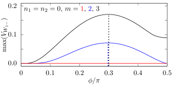
Figure 3: The maximum achievable $V_{W_{1-}}$ as a function of $\phi$ for the MPJC model with both the oscillators initially in the ground states and where the qubit is initially in a superposition state $\cos\phi\ket{g}+\sin\phi\ket{e}$ with $m=$ 1 (red), 2 (blue), and 3 (red), respectively. Similar to Fig. 2, we set $g_{1}=g_{2}=1/\sqrt{2}$ and $\Delta=0$. For $m=1$ (tripartite JC interactions), the Wigner function of the oscillator remains positive at all times for all values of $\phi$. The dashed horizontal lines indicate the values of $\phi$ (both very close to $\pi/6$) for which the corresponding curves attain the highest value.

Furthermore, noteworthy enhancements in the initial Wigner negativity of Fock states $\ket{1}$ and $\ket{2}$ of the first oscillator are achieved during nonlinear evolution, as evidenced by the black and red curves in Fig. 2 for both values of $\phi$. Interestingly, in contrast to $\phi=\pi/4$, the red and black curves for $\phi=\pi/2$ can dip below their initial value during the evolution. Comparing the red curves in both panels, we observe that the extent of $V_{W_{1-}}$ is much higher for $\phi=\pi/4$ than for $\phi=\pi/2$. We have numerically verified that apart from these specific combinations, such enhancements in $V_{W_{1-}}$ are also present for other combinations of $n_{1}$, $n_{2}$, and $m$ that fall under case 1. Similar to $n_{1}=n_{2}=0$, we find that the nonlinearity introduced by $m$ significantly impacts whether the initial nonclassicality is surpassed.

Case 2: Now, let us examine case 2, where $n_{1}<n_{2}=m$ or $n_{2}<n_{1}=m$. The time-evolved Wigner function of the first oscillator is found to be (see Appendix C for details)

$$\tilde{W}_{1}(\alpha,t) =(-1)^{n_{1}}\Big{[}\left(|x_{1}|^{2}+|x_{2}|^{2}+|y_{1}|^{2}+|y_{3}|^{2}\right)L_{n_{1}}(z)$$

$$+(-1)^{m}\left(|x_{3}|^{2}+|y_{2}|^{2}+|y_{4}|^{2}\right)L_{n_{1}+m}(z)$$

$$+2^{m}\sqrt{\tfrac{n_{1}!}{(n_{1}+m)!}}\big{(}\alpha^{m}\left(x_{1}y_{2}^{*}+x_{2}y_{4}^{*}\right)+\text{h.c.}\big{)}L_{n_{1}}^{m}(z)$$

$$+(-2)^{m}\sqrt{\tfrac{(n_{1}+m)!}{(n_{1}+2m)!}}\left(x_{3}y_{5}^{*}\alpha^{m}+\text{h.c.}\right)L_{n_{1}+m}^{m}(z)$$

$$+|y_{5}|^{2}L_{n_{1}+2m}(z)\Big{]}.$$ (30)

Here, h.c. stands for hermitian conjugate. Unlike the previous case, now the Wigner function does not remain constant for $\phi=0$ (that is when all $y$ coefficients become zero), instead, it has the form

$$\tilde{W}_{1}(\alpha,t) =(-1)^{n_{1}}\Big{[}\left(1-|x_{3}|^{2}\right)L_{n_{1}}(z)$$

$$\hskip 46.97505pt+(-1)^{m}|x_{3}|^{2}L_{n_{1}+m}(z)\Big{]}.$$ (31)

This results in a nontrivial evolution of $V_{W_{1-}}$ in contrast to case 1, as depicted in Fig. 4(a). Now, if we assume that the first oscillator is prepared in the ground state $(n_{1}=0)$, we get

$$\tilde{W}_{1}(\alpha,t)=(-1)^{n_{1}}\left[1-|x_{3}|^{2}+(-1)^{m}|x_{3}|^{2}L_{m}(z)\right].$$ (32)

Therefore, whenever $|x_{3}|^{2}=1$, we obtain $W_{1}(\alpha,t)=\frac{2}{\pi}\,e^{-2|\alpha|^{2}}(-1)^{n_{1}}L_{m}\left(4|\alpha|^{2}\right)=W_{2}(\alpha,0)$. As a result, $V_{W_{1-}}$ periodically attains the value of the initial $V_{W_{2-}}$ of the second oscillator (perfect Fock state swapping as discussed in the preceding Section), as demonstrated by the blue curve in Fig. 4(a). Additionally, we observe that the enhancements in $V_{W_{1-}}$ diminish as the initial mean photon number of the first oscillator $n_{1}$ increases. Specifically, for $n_{1}=2,\,n_{2}=m=3$ and also for $n_{1}=m=3,\,n_{2}=2$ (corresponding to the situation $n_{2}<n_{1}=m$), no enhancements from their initial values are observed (as represented by the red and yellow curves respectively in Fig. 4(a)). This occurs because, with a gradual increase in the value of $n_{1}$, the amplitude of $x_{3}$ decreases, suggesting a gradual reduction in the purity of the oscillator state, as previously explained (see Eqs.(21) and (22)).

On the other hand, when $\phi=\pi/2$, the $x$ coefficients vanish, significantly simplifying Eq. (30), yielding

$$\tilde{W}_{1}(\alpha,t) =(-1)^{n_{1}}\Big{[}\left(|y_{1}|^{2}+|y_{3}|^{2}\right)L_{n_{1}}(z)$$

$$\hskip 31.07556pt+(-1)^{m}\left(|y_{2}|^{2}+|y_{4}|^{2}\right)L_{n_{1}+m}(z)$$

$$\hskip 31.07556pt+|y_{5}|^{2}L_{n_{1}+2m}(z)\Big{]}.$$ (33)

Now, for the simple case when $n_{1}=0$, the above expression becomes

$$\tilde{W}_{1}(\alpha,t) =|y_{1}|^{2}+|y_{3}|^{2}+(-1)^{m}\left(|y_{2}|^{2}+|y_{4}|^{2}\right)L_{m}(z)$$

$$\hskip 21.68121pt+|y_{5}|^{2}L_{2m}(z).$$ (34)

This clearly indicates that the initial ground state oscillator becomes nonclassical and the degree of the nonclassicality should increase with increasing $n_{2}=m$ value. We have numerically verified this, and the blue curve in panel (c) of Fig. 4 illustrates the corresponding behavior when $n_{2}=m=3$. It is evident that the nonclassicality exceeds the corresponding value of $\ket{5}$ (dashed magenta line in panel (c)). For other combinations of $n_{1}$, $n_{2}$, and $m$, the dynamics appear to be similarly complex for this case with comparatively lesser enhancement in their respective initial degree of nonclassicality.

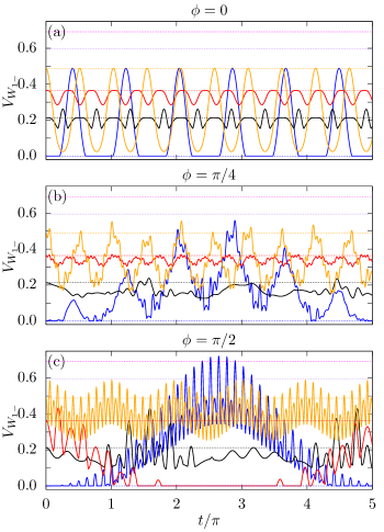
Figure 4: The nonlinear evolution of $V_{W_{1-}}$ of the first oscillator for case 2 (that is, when $n_{1}<n_{2}=m$ or $n_{2}<n_{1}=m$) for $\phi=0$ (a), $\pi/4$ (b), and $\pi/2$ (c), respectively. For all the panels, the initial states of the first oscillator are $\ket{0}$ (blue), $\ket{1}$ (black), $\ket{2}$ (red), and $\ket{3}$ (yellow). Further, for the blue, black, red and yellow curves, the respective values of $(n_{2},\,m)$ are (3, 3), (3, 3), (3, 3), and (1, 3) for panel (a), and (3, 3), (2, 2), (3, 3), and (1, 3) for panel (b), while for panel (c), the values are (3, 3), (2, 2), (0, 2), and (1, 3). Similar to Fig. 2, we set $g_{1}=g_{2}=1/\sqrt{2}$ and $\Delta=0$. The dashed horizontal lines correspond to $V_{W_{1-}}$ of the initial Fock states.

Lastly, for values of $\phi$ other than 0 and $\pi/2$, all the $x$ and $y$ coefficients contribute to the dynamics, leading to a notably intricate temporal evolution of $V_{W_{1-}}$ (see panel (b) of Fig. 4). We notice that the enhancements in $V_{W_{1-}}$ are smaller unless $n_{1}=0$. These inferences hold true for all combinations of $n_{1}$, $n_{2}$, and $m$ in this case, with the most significant ones depicted in Fig. 4.

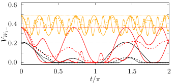
Figure 5: The nonlinear evolution of $V_{W_{1-}}$ of the first oscillator for case 3, that is when $n_{1}=n_{2}=m=$ 1 (black), 2 (red), and 3 (yellow) with $\phi=0$ (solid), $\pi/4$ (dashed), and $\pi/2$ (dotted), respectively. Similar to Fig. 2, we set $g_{1}=g_{2}=1/\sqrt{2}$ and $\Delta=0$. Unlike the previous two cases, in this scenario, the nonlinear evolution fails to surpass the initial nonclassicality of the oscillator, at best $V_{W_{1-}}$ returns to its initial value at periodic intervals.

Cases 3 and 4: We now move on to case 3, where $n_{1}=n_{2}=m$. The exact analytical expression for $W_{1}(\alpha,t)$ can be found in Appendix C. The temporal evolution of $V_{W_{1-}}$ of the first oscillator is illustrated in Fig. 4. In complete contrast to the previous two cases, in this case, we do not observe any surpassing of the initial nonclassicality for any value of $\phi$. At best, $V_{W_{1-}}$ returns to its initial value at periodic intervals. This can be explained analytically for $\phi=0$. As mentioned in the previous Section, the oscillator state $\ket{m}$ (to be precise, $|x_{1}|^{2}$) returns to itself periodically for this scenario. On the other hand, the analytical expressions for the Wigner functions of the two oscillators for case 4 can also be found in Appendix C. Similar to case 3, we have numerically verified that surpassing the initial nonclassicality for any value of $\phi$ is absent for this case as well.

In summary, after examining all four cases, we conclude that the multiphoton parameter $m$ plays a crucial role in surpassing the initial nonclassicalities of the photon number states. In particular, we observe that $m$ should be at least greater than the mean photon number of one of the oscillators to achieve higher than the initial Wigner nonclassicality.

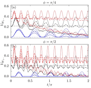
Figure 6: The role of environmentally induced decoherence and dephasing effects on $V_{W_{1-}}$ of the first oscillator for case 1 (as shown in Fig. 2) is illustrated for $\bar{n}_{\text{th}}=0$. In both panels, the large (small) dashed curves represent the temporal evolution in the presence of dissipation (dephasing) only, i.e., $\lambda_{d}=0$ ($\lambda_{r}=0$) with $\lambda_{r}=0.05$ ($\lambda_{d}=0.05$), while the dotted curves depict the cumulative effects of both dissipation and dephasing ($\lambda_{r}=\lambda_{d}=0.05$). The solid curves correspond to unitary dynamics (Fig. 2). The horizontal dashed-dotted lines correspond to the initial nonclassicality of the Fock states.

V.1 Robustness of $V_{W_{1-}}$ against environmental effects

Even with the tremendous experimental progress in harnessing and isolating quantum systems from environmentally induced effects, shielding the system entirely remains a challenge in any realistic quantum platform. So far in our analysis, we have ignored such contributions completely. In this Section, we are going to numerically estimate the degree to which the nonclassicalities in Fock states are affected by considering realistic system-environmental coupling parameters. In the Lindblad formalism, the evolution of the tripartite system’s density matrix $\rho_{S}(t)$ is described by the standard master equation

$$\displaystyle\frac{d\rho_{S}}{dt}=-i\left[H,\rho_{S}\right]+\sum_{k}\lambda_{k}\left(A_{k}\rho_{S}A_{k}^{\dagger}-\frac{1}{2}\left[\rho_{S},A_{k}^{\dagger}A_{k}\right]\right).$$ (35)

Here, the environment couples to the system via the operators $A_{k}$ with coupling rates $\lambda_{k}$. We assume a common thermal environment for the entire system with thermal energy $\bar{n}_{\text{th}}$ for simplicity. For dissipation, we consider Lindblad operators $a_{i}$ and $\sigma_{-}$ with dissipation rates $\sqrt{\lambda_{r}(1+\bar{n}_{\text{th}})}$, where $i=1,\,2$. We also set equal coupling coefficients to simplify the analysis. Similarly, for relaxation, the Lindblad operators are $a_{i}^{\dagger}$ and $\sigma_{+}$ with relaxation rates $\sqrt{\lambda_{r}\bar{n}_{\text{th}}}$. Additionally, we include the effect of dephasing through environmental interactions. Here, the relevant Lindblad operators are $a_{i}^{\dagger}a_{i}$ and $\sigma_{z}$ with equal coupling rate $\sqrt{\lambda_{d}}$, which does not depend on $\bar{n}_{\text{th}}$. We keep in mind that, in the asymptotic limit, all states converge to a thermal state with no negativity in the Wigner function.

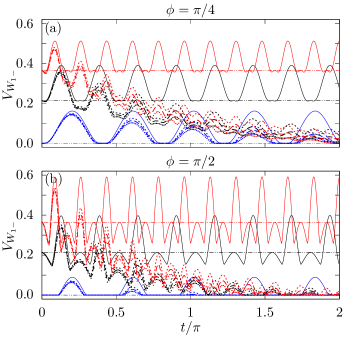
Figure 7: The role of thermal environment on $V_{W_{1-}}$ of the first oscillator for case 1 (as shown in Fig. 2). In both panels, the small dashed, the large dashed and the dotted curves correspond to $\bar{n}_{\text{th}}=0$, 0.1, and 0.2, respectively. Further, $\lambda_{r}=0.05$, $\lambda_{d}=0$. The solid curves correspond to unitary dynamics (Fig. 2).

We begin by assuming $\bar{n}_{\text{th}}=0$, indicating that the system interacts with a vacuum environment. The relevant Lindblad operators are $a_{i}$, $\sigma_{-}$, $a_{i}^{\dagger}a_{i}$ and $\sigma_{z}$. In Fig. 6, we illustrate the detrimental effects of the environment on the temporal evolution of $V_{W_{1-}}$ corresponding to case 1. We consider three sources of losses: (i) pure dissipation ($\lambda_{r}=0.05$, $\lambda_{d}=0$), (ii) pure dephasing ($\lambda_{r}=0$, $\lambda_{d}=0.05$), and (iii) the combined effect of dissipation and dephasing ($\lambda_{r}=0.05$, $\lambda_{d}=0.05$). These are represented by the large dashed, small dashed, and dotted curves, respectively, in Fig. 6. It is evident that dissipation losses outweigh dephasing in most scenarios, except when $\phi=\pi/4$ and $n_{1}=0$ (blue dashed curves in Fig. 6(a)). Moreover, we find that the higher initial Fock states are more susceptible to noise, as expected.

The role of the temperature of the thermal bath $\bar{n}_{\text{th}}$ on the temporal evolution of $V_{W_{1-}}$ is investigated in Fig. 7. Here, all the Lindblad operators contribute to the dynamics. As expected, increasing the temperature of the thermal bath results in a faster reduction in nonclassicality. Similar to Fig. 6, the nonclassicality of the higher Fock states degrades much faster.

VI Conclusions

To conclude, we have found and explored the analytical solution of the time-evolved state vector of the tripartite $m$-photon Jaynes-Cummings system considering a pure initial state in which the qubit is in a superposition state and the two quantized harmonic oscillators are in arbitrary Fock states $\ket{n_{1}}$ and $\ket{n_{2}}$, respectively. Depending on the specific values of $n_{1}$, $n_{2}$, and $m$, we have identified four different cases and obtained exact analytical solutions for most of them. Furthermore, we have analytically extracted the time-evolved oscillator states by tracing over the relevant subsystems and shown that perfect swapping of Fock states between the oscillators can be achieved under carefully chosen system parameters. While swapping the states of quantum optical modes is also achievable through suitable beamsplitter interactions, here such swapping is the result of an exact analytical evolution of a fairly complicated, tripartite, nonlinear spin-boson Hamiltonian.

In the latter half of the article, we have carried out a detailed analysis of how the nonclassicalities of the initial oscillator Fock states evolve under such nonlinear Hamiltonian evolution considering diverse system parameters. Following previous work [51, 52], we quantified the degree of nonclassicality of a quantum state by the volume of the negative regions of its corresponding Wigner function. Besides producing substantial enhancements in the initial value for higher photon number states, our analysis reveals that the nonlinear MPJC interaction, driven solely by the initial qubit energy (with both the oscillators initialized in the vacuum state), yields nontrivial Wigner negativities in the oscillators. Interestingly, it turns out that the additional nonlinearity of the multiphoton interactions $m$ dictates the eventual outcome of surpassing the initial nonclassicalities of the photon number states.

For completeness, we have also tested the robustness of such nonclassicalities under additional environmentally induced interactions and the role of imperfect matching of frequencies between the discrete and continuous variable quantum systems on the Wigner nonclassicalities. It would be interesting to conduct a similar analysis incorporating other initial qubit and oscillator states, including incoherent ones. The numerical results presented in this paper are obtained using the qutip library [55].

Finally, we have also explored the squeezing properties of time-evolved oscillator states across all four distinct cases. Our findings reveal that none of the oscillators exhibit any conventional quadrature squeezing. However, the highly nonclassical nature of these states suggests the potential for squeezing extraction through various distillation techniques [56]. Investigating the extent of distillable squeezing, if present, remains an interesting exercise. Additionally, from a theoretical standpoint, the next logical step would involve probing these phenomena within the multiphoton rendition of the standard double Jaynes-Cummings system, which includes two qubits and two oscillators [57].

Having obtained the reduced oscillator states by tracing over the relevant subsystems, which tends to reduce the purity of the quantum states, a natural next step would involve transitioning from this deterministic approach to a probabilistic one. This would entail obtaining the target oscillator state by measuring the qubit and the remaining oscillator. Another facet of the study involves examining the dynamics of bosonic entanglement between the oscillators and qubit coherence, two of the most prominent resources in modern quantum technology. This aspect has already been extensively addressed in Ref. [50].

Apart from advancing our theoretical understanding of the role of multiphoton interactions on various nonclassical phenomena, we believe that the results presented in this work will provide significant impetus to already rapidly evolving experimental exploration with multiphoton processes in various quantum platforms [58, 59, 60], and potentially contribute to the ultimate applications in photonic quantum technology, involving universal and fault-tolerant processing, where most advanced, nonclassical, non-Gaussian optical quantum states are required.

Appendix A The $M$ matrices

Case 2: Given below are the expressions for the $M$ matrices for case 2:

$$M_{2_{x}}=\begin{pmatrix}-\Delta^{\prime}&g_{2_{m}}&0\\ g_{2_{m}}&\Delta^{\prime}&g_{1_{n_{1}m}}\\ 0&g_{1_{n_{1}m}}&-\Delta^{\prime}\end{pmatrix},$$ (36)

where $\Delta^{\prime}=\Delta/2$, $g_{1_{n_{1}m}}=\sqrt{(n_{1}+m)!/n_{1}!}\,g_{1}$, $g_{2_{m}}=\sqrt{m!}\,g_{2}$, and

$$M_{2_{y}}=\begin{pmatrix}\Delta^{\prime}&g_{1_{n_{1}m}}&g^{\prime}_{2_{m}}&0&0\\ g_{1_{n_{1}m}}&-\Delta^{\prime}&0&g_{2_{m}}&0\\ g^{\prime}_{2_{m}}&0&-\Delta^{\prime}&0&0\\ 0&g_{2_{m}}&0&\Delta^{\prime}&g^{\prime}_{1_{n_{1}m}}\\ 0&0&0&g^{\prime}_{1_{n_{1}m}}&-\Delta^{\prime}\end{pmatrix},$$ (37)

where $g^{\prime}_{2_{m}}=\sqrt{(2m)!/m!}\,g_{2}$, and $g^{\prime}_{1_{n_{1}m}}=\sqrt{(n_{1}+2m)!/(n_{1}+m)!}\,g_{1}$.

Case 3: Given below are the expressions for the $M$ matrices for case 3:

$$M_{3_{x}}=\begin{pmatrix}-\Delta^{\prime}&g_{1_{m}}&g_{2_{m}}&0&0\\ g_{1_{m}}&\Delta^{\prime}&0&g^{\prime}_{2_{m}}&0\\ g_{2_{m}}&0&\Delta^{\prime}&0&g^{\prime}_{1_{m}}\\ 0&g^{\prime}_{2_{m}}&0&-\Delta^{\prime}&0\\ 0&0&g^{\prime}_{1_{m}}&0&-\Delta^{\prime}\end{pmatrix},$$ (38)

where $g_{1_{m}}=\sqrt{m!}g_{1}$, $g^{\prime}_{1_{m}}=\sqrt{(2m)!/m!}g_{1}$, and

$$M_{3_{y}}=\begin{pmatrix}\Delta^{\prime}&g^{\prime}_{1_{m}}&g^{\prime}_{2_{m}}&0&0&0&0\\ g^{\prime}_{1_{m}}&-\Delta^{\prime}&0&g_{2_{m}}&0&0&0\\ g^{\prime}_{2_{m}}&0&-\Delta^{\prime}&0&g_{1_{m}}&0&0\\ 0&g_{2_{m}}&0&\Delta^{\prime}&0&g^{\prime\prime}_{1_{m}}&0\\ 0&0&g_{1_{m}}&0&\Delta^{\prime}&0&g^{\prime\prime}_{2_{m}}\\ 0&0&0&g^{\prime\prime}_{1_{m}}&0&-\Delta^{\prime}&0\\ 0&0&0&0&g^{\prime\prime}_{2_{m}}&0&-\Delta^{\prime}\end{pmatrix},$$ (39)

where $g^{\prime\prime}_{1_{m}}=\sqrt{(3m)!/(2m)!}g_{1}$, and $g^{\prime\prime}_{2_{m}}=\sqrt{(3m)!/(2m)!}g_{2}$.

The reduced density matrices for the two oscillators in the effective basis states $\ket{0}$, $\ket{m}$, $\ket{2m}$, and $\ket{3m}$ are given by

$$\rho_{1}^{(3)}=\begin{pmatrix}|x_{2}|^{2}+|x_{5}|^{2}+|y_{5}|^{2}+|y_{7}|^{2}&x_{2}y_{1}^{*}+x_{5}y_{3}^{*}&0&0\\ x_{2}^{*}y_{1}+x_{5}^{*}y_{3}&|x_{1}|^{2}+|x_{3}|^{2}+|y_{1}|^{2}+|y_{3}|^{2}&x_{1}y_{2}^{*}+x_{3}y_{4}^{*}&0\\ 0&x_{1}^{*}y_{2}+x_{3}^{*}y_{4}&|x_{4}|^{2}+|y_{2}|^{2}+|y_{4}|^{2}&x_{4}y_{6}^{*}\\ 0&0&x_{4}^{*}y_{6}&|y_{6}|^{2}\end{pmatrix},$$ (40)

and

$$\rho_{2}^{(3)}=\begin{pmatrix}|x_{3}|^{2}+|x_{4}|^{2}+|y_{4}|^{2}+|y_{6}|^{2}&x_{3}y_{1}^{*}+x_{4}y_{2}^{*}&0&0\\ x_{3}^{*}y_{1}+x_{4}^{*}y_{2}&|x_{1}|^{2}+|x_{2}|^{2}+|y_{1}|^{2}+|y_{2}|^{2}&x_{1}y_{3}^{*}+x_{2}y_{5}^{*}&0\\ 0&x_{1}^{*}y_{3}+x_{2}^{*}y_{5}&|x_{5}|^{2}+|y_{3}|^{2}+|y_{5}|^{2}&x_{5}y_{7}^{*}\\ 0&0&x_{5}^{*}y_{7}&|y_{7}|^{2}\end{pmatrix}.$$ (41)

Case 4: The exact forms of the state vectors $\ket{\psi_{x}(t)}_{4}$ and $\ket{\psi_{y}(t)}_{4}$ are given by

$$\ket{\psi_{x}(t)}_{4} =\sum_{k=0}^{\ell_{2}-1}\Big{(}x_{4k+1}\ket{g,\,n_{1}+km,\,n_{2}-km}$$

$$+x_{4k+3}\ket{e,\,n_{1}+km,\,n_{2}-(k+1)m}\Big{)}$$

$$+\sum_{k=0}^{\ell_{1}-2}\Big{(}x_{4k+2}\ket{e,\,n_{1}-(k+1)m,\,n_{2}+km}$$

$$+x_{4k+4}\ket{g,\,n_{1}-(k+1)m,\,n_{2}+(k+1)m}\Big{)},$$ (42)

and

$$\ket{\psi_{y}(t)}_{4} =\sum_{k=0}^{\ell_{2}-1}\Big{(}y_{4k+1}\ket{e,\,n_{1}-km,\,n_{2}+km}$$

$$+y_{4k+3}\ket{g,\,n_{1}-km,\,n_{2}+(k+1)m}\Big{)}$$

$$+\sum_{k=0}^{\ell_{1}-1}\Big{(}y_{4k+2}\ket{g,\,n_{1}+(k+1)m,\,n_{2}-km}$$

$$+y_{4k+4}\ket{e,\,n_{1}+(k+1)m,\,n_{2}-(k+1)m}\Big{)},$$ (43)

respectively. Note that for this case $\ell_{1},\,\ell_{2}>2$, as $\min(m)=1$. As mentioned earlier, $\ket{\psi_{x}(t)}_{4}$ and $\ket{\psi_{y}(t)}_{4}$ contains $2\ell_{1}+2\ell_{2}-3$ and $2\ell_{1}+2\ell_{2}-1$) basis states respectively with $\ell_{i}$ representing the smallest positive integer for which $n_{i}-\ell_{i}m<0$ ($i=1,\,2$).

The two $M$ matrices assume symmetric pentadiagonal structures. The nonzero elements of the upper half including the diagonal elements are given below:

$$\left(M_{4_{x}}\right)_{i,i} =\left\{\begin{array}[]{rcl}-\Delta^{\prime}&\mbox{for}&i=4k+1,4k+4\\ \Delta^{\prime}&\mbox{for}&i=4k+2,4k+3,\end{array}\right.,$$ (46)

$$\left(M_{4_{x}}\right)_{0,1} =\sqrt{\tfrac{n_{1}!}{(n_{1}-m)!}}g_{1},$$

$$\left(M_{4_{x}}\right)_{i,i+2} =\left\{\begin{array}[]{rcl}\sqrt{\frac{(n_{2}-j_{1}m)!}{(n_{2}-(j_{1}+1)m)!}}g_{2}&\mbox{for}&i=4k+1,\\ \sqrt{\frac{(n_{2}+j_{2}m)!}{(n_{2}+(j_{2}-1)m)!}}g_{2}&\mbox{for}&i=4k+2,\\ \sqrt{\frac{(n_{1}+j_{2}m)!}{(n_{1}+(j_{2}-1)m)!}}g_{1}&\mbox{for}&i=4k+3,\\ \sqrt{\frac{(n_{1}-j_{1}m)!}{(n_{1}-(j_{1}+1)m)!}}g_{1}&\mbox{for}&i=4k+4,\end{array}\right..$$ (51)

Here, $j_{1}=\lfloor\frac{i}{4}\rfloor$, $j_{2}=\lceil\frac{i}{4}\rceil$, and $k=0,\,1,\,2,\ldots$. Note that $\lfloor\cdot\rfloor$ and $\lceil\cdot\rceil$ denote floor and ceiling functions, respectively. Similarly, we can show that

$$\left(M_{4_{y}}\right)_{i,i} =\left\{\begin{array}[]{rcl}\Delta^{\prime}&\mbox{for}&i=4k+1,4k+4\\ -\Delta^{\prime}&\mbox{for}&i=4k+2,4k+3,\end{array}\right.,$$ (54)

$$\left(M_{4_{y}}\right)_{0,1} =\sqrt{\tfrac{(n_{1}+m)!}{n_{1}!}}g_{1},$$

$$\left(M_{4_{y}}\right)_{i,i+2} =\left\{\begin{array}[]{rcl}\sqrt{\frac{(n_{2}+j_{2}m)!}{(n_{2}+(j_{2}-1)m)!}}g_{2}&\mbox{for}&i=4k+1,\\ \sqrt{\frac{(n_{2}-j_{1}m)!}{(n_{2}-(j_{1}+1)m)!}}g_{2}&\mbox{for}&i=4k+2,\\ \sqrt{\frac{(n_{1}-j_{1}m)!}{(n_{1}-(j_{1}+1)m)!}}g_{1}&\mbox{for}&i=4k+3,\\ \sqrt{\frac{(n_{1}+(j_{1}+1)m)!}{(n_{1}+j_{1}m)!}}g_{1}&\mbox{for}&i=4k+4,\end{array}\right..$$ (59)

The time-evolved reduced state of the first oscillator for this case is given by

$$\rho_{1}^{(4)}(t) =\sum_{k=0}^{k_{\text{max}}}\big{[}\rho_{n_{1}+km,\,n_{1}+km}\ket{n_{1}+km}\bra{n_{1}+km}$$

$$\,\,\,+\rho_{n_{1}-km,\,n_{1}-km}\ket{n_{1}-km}\bra{n_{1}-km}$$

$$\,\,\,+\big{(}\rho_{n_{1}+km,\,n_{1}+(k+1)m}\ket{n_{1}+km}\bra{n_{1}+(k+1)m}$$

$$\,\,\,+\rho_{n_{1}-(k+1)m,\,n_{1}-km}\ket{n_{1}-(k+1)m}\bra{n_{1}-km}$$

$$\,\,\,+\text{h.c.}\big{)}\big{]},$$ (60)

where $\rho_{n_{1}+km,\,n_{1}+km}=|x_{4k+1}|^{2}+|x_{4k+3}|^{2}+|y_{4k-2}|^{2}+|y_{4k}|^{2}$, $\rho_{n_{1}-km,\,n_{1}-km}=|x_{4k-2}|^{2}+|x_{4k}|^{2}+|y_{4k+1}|^{2}+|y_{4k+3}|^{2}$, $\rho_{n_{1}+km,\,n_{1}+(k+1)m}=x_{4k+1}y^{*}_{4k+2}+x_{4k+3}y^{*}_{4k+4}$, $\rho_{n_{1}-(k+1)m,\,n_{1}-km}=x_{4k+4}y^{*}_{4k+3}+x_{4k+2}y^{*}_{4k+1}$. Further, $k_{\text{max}}=\max(\ell_{1}-1,\ell_{2}-1)$.

Similarly, for the second oscillator, we get

$$\rho_{2}^{(4)}(t) =\sum_{k=0}^{k_{\text{max}}}\big{[}\rho_{n_{2}-km,\,n_{2}-km}\ket{n_{2}-km}\bra{n_{2}-km}$$

$$\,\,\,+\rho_{n_{2}+km,\,n_{2}+km}\ket{n_{2}+km}\bra{n_{2}+km}$$

$$\,\,\,+\big{(}\rho_{n_{2}-(k+1)m,\,n_{2}-km}\ket{n_{2}-(k+1)m}\bra{n_{2}-km}$$

$$\,\,\,+\rho_{n_{2}+km,\,n_{2}+(k+1)m}\ket{n_{2}+km}\bra{n_{2}+(k+1)m}$$

$$\,\,\,+\text{h.c.}\big{)}\Big{]}+\big{(}\rho_{n_{2},\,n_{2}+m}\ket{n_{2}}\bra{n_{2}+m}$$

$$\,\,\,+\rho_{n_{2},\,n_{2}-m}\ket{n_{2}}\bra{n_{2}-m}+\text{h.c.}\big{)},$$ (61)

where $\rho_{n_{2}-km,\,n_{2}-km}=|x_{4k+1}|^{2}+|y_{4k+2}|^{2}+|x_{4k-1}|^{2}+|y_{4k}|^{2}$, $\rho_{n_{2}+km,\,n_{2}+km}=|x_{4k}|^{2}+|y_{4k-1}|^{2}+|x_{4k+2}|^{2}+|y_{4k+1}|^{2}$, $\rho_{n_{2}-(k+1)m,\,n_{2}-km}=x_{4k+5}y_{4k+2}^{*}+x_{4k+3}y^{*}_{4k}$, $\rho_{n_{2}+km,\,n_{2}+(k+1)m}=x_{4k}y^{*}_{4k+3}+x_{4k+2}y^{*}_{4k+5}$, $\rho_{n_{2},\,n_{2}+m}=x_{1}y_{3}^{*}+x_{4}^{*}y_{2}$, and $\rho_{n_{2},\,n_{2}-m}=x_{2}y_{4}^{*}+y_{1}x_{3}^{*}$. As before, $k_{\text{max}}=\max(\ell_{1}-1,\ell_{2}-1)$.

Appendix B The role of detuning $\Delta$

Thus far in our analysis of the volume of the Wigner negativities $V_{W_{1-}}$, we have always assumed perfect matching of frequencies between the qubit and the oscillators, that is $\Delta=0$. Here, we examine the changes that manifest in $V_{W_{1-}}$ when there is imperfect matching of frequencies.

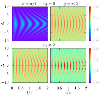
Figure 8: The Wigner nonclassicality of the first oscillator $V_{W_{1-}}$ is displayed as functions of time and the detuning $\Delta$ for case 1. In all panels, $m=3$ and $n_{2}=0$. The first and second columns represent $\phi=\pi/4$ and $\phi=\pi/2$, respectively, while the first and second rows correspond to $n_{1}=0$ and 2, respectively. As previously mentioned, $g_{1}=g_{2}=1/\sqrt{2}$.

For case 1, this is illustrated in Fig. 8. Both from Eq.(9) and Fig. 8, it is evident that for fixed values of $n_{1}$, $n_{2}$ and $m$, the detuning $\Delta$ increases the periodicity and simultaneously decreases the amplitude of the oscillations. In particular, the farther we move away from perfect resonance ($\Delta=0$), the lower the degree of nonclassicality. Eventually, in the dispersive limit, i.e., when $\Delta\gg g_{1},g_{2}$, the nonclassicality vanishes almost entirely. This is consistent with the expected behavior in the dispersive regime [61]. Similar to case 1, we have numerically verified that the qualitative changes in the behavior of $V_{W_{1-}}$ due to nonzero detuning also remain similar for other cases.

Appendix C Derivations of the Wigner functions

In this Section, we give details on analytically deriving the Wigner functions of the time-evolved oscillator states. For any generic quantum state $\varrho$, characterized by its bosonic annihilation and creation operators $a$ and $a^{\dagger}$, the associated Wigner function $W(\alpha)$ is conventionally defined as [62, 63]

$$W(\alpha) =\frac{1}{\pi}{\rm Tr}\,\left[\varrho\,T(\alpha)\right],$$ (62)

where

$$T(\alpha)=\int\frac{d^{2}\xi}{\pi}\,\exp{(\alpha\xi^{*}-\alpha^{*}\xi)}D(\xi),$$ (63)

is a hermitian operator and $D(\xi)=\exp(\xi a^{\dagger}-\xi^{*}a)$ is the standard displacement operator. The elements of the hermitian matrix $T(\alpha)$ in the number basis are given by [62]

$$\braket{k_{1}}{T(\alpha)}{k_{2}}=2(-1)^{k_{1}}e^{-2|\alpha|^{2}} \sqrt{\tfrac{k_{1}!}{k_{2}!}}\,(2\alpha^{*})^{k_{2}-k_{1}}$$

$$\times L_{k_{1}}^{k_{2}-k_{1}}\left(4|\alpha|^{2}\right),$$ (64)

for $k_{2}\geq k_{1}$, and

$$\braket{k_{1}}{T(\alpha)}{k_{2}}=2(-1)^{k_{2}}e^{-2|\alpha|^{2}} \sqrt{\tfrac{k_{2}!}{k_{1}!}}\,(2\alpha)^{k_{1}-k_{2}}$$

$$\times L_{k_{2}}^{k_{1}-k_{2}}\left(4|\alpha|^{2}\right),$$ (65)

for $k_{2}<k_{1}$. Here, $L_{k_{1}}^{k_{2}}(x)$ is the associated Laguerre polynomial.

Case 1: The reduced density matrices of the two oscillators in this case ($n_{1},\,n_{2}<m$) are given by Eqs.(17) and (18), respectively. Since only two basis states $\ket{n_{i}}$ and $\ket{n_{i}+m}$ are involved for both oscillators in this case ($i=1,\,2$), we can easily obtain the associated Wigner functions following the above procedure. For the second oscillator, we have

$$W_{2}(\alpha,t) =\frac{1}{\pi}\big{[}(|x_{1}|^{2}+|y_{1}|^{2}+|y_{2}|^{2})\langle n_{2}|T(\alpha)|n_{2}\rangle$$

$$+\left(x_{1}y_{3}^{*}\langle n_{2}+m|T(\alpha)|n_{2}\rangle+\text{h.c.}\right)$$

$$+|y_{3}|^{2}\langle n_{2}+m|T(\alpha)|n_{2}+m\rangle\big{]}.$$ (66)

Now, using Eqs.(64) and (65), we finally obtain

$$\tilde{W}_{2}(\alpha,t) =(-1)^{n_{2}}\left[\left(|x_{1}|^{2}+|y_{1}|^{2}+|y_{2}|^{2}\right)L_{n_{2}}(z)\right.$$

$$+2^{m}\sqrt{\tfrac{n_{2}!}{(n_{2}+m)!}}\left(x_{1}y_{3}^{*}\alpha^{m}+y_{3}x_{1}^{*}(\alpha^{*})^{m}\right)L_{n_{2}}^{m}(z)$$

$$+\left.(-1)^{m}|y_{3}|^{2}L_{n_{2}+m}(z)\right],$$ (67)

where $\tilde{W}_{2}(\alpha,t)=\frac{2}{\pi}e^{-2|\alpha|^{2}}W_{2}(\alpha,t)$, and $z=4|\alpha|^{2}$ as usual. Following a similar procedure, we also obtain the Wigner function of the first oscillator and it is given by Eq.(25).

Case 2: The reduced density matrices of the two oscillators in this case ($n_{1}<n_{2}=m$) are given by Eq.(19) and Eq.(20), respectively. Here, only three basis states are involved for both oscillators. The associated Wigner function for the first oscillator is given by Eq.(30) while for the second oscillator, we have

$$\tilde{W}_{2}(\alpha,t) =\left(|x_{2}|^{2}+|x_{3}|^{2}+|y_{4}|^{2}+|y_{5}|^{2}\right)L_{n_{2}}(z)$$

$$+(-1)^{m}\left(|x_{1}|^{2}+|y_{1}|^{2}+|y_{2}|^{2}\right)L_{n_{2}+m}(z)$$

$$+2^{m}\sqrt{\tfrac{n_{2}!}{n_{2}+m!}}\left\{\left(x_{2}y_{1}^{*}+x_{3}y_{2}^{*}\right)\alpha^{m}+\text{h.c.}\right\}L_{n_{2}}^{m}(z)$$

$$+(-2)^{m}\sqrt{\tfrac{n_{2}+m!}{(n_{2}+2m)!}}\left(x_{1}y_{3}^{*}\alpha^{m}+\text{h.c.}\right)L_{n_{2}+m}^{m}(z)$$

$$+|y_{3}|^{2}L_{n_{2}+2m}(z).$$ (68)

Case 3: For this case, the reduced density matrices for the two oscillators are given by Eqs.(40) and (41), respectively. The associated Wigner function for both oscillators can be expressed as

$$\tilde{W}(\alpha,t) =\rho_{0,0}+\rho_{2m,2m}L_{2m}(z)+(-1)^{m}\big{\{}\rho_{m,m}L_{m}(z)$$

$$\,\,\,+\rho_{3m,3m}L_{3m}(z)\big{\}}+(2\alpha)^{m}\Big{[}\tfrac{1}{\sqrt{m!}}\,\rho_{0,m}$$

$$\,\,\,+(-1)^{m}\sqrt{\tfrac{m!}{(2m)!}}\,\rho_{m,2m}L_{m}^{m}(z)$$

$$\,\,\,+\sqrt{\tfrac{(2m)!}{(3m)!}}\,\rho_{2m,3m}L_{2m}^{m}(z)+{\rm h.c.}\Big{]},$$ (69)

where $\rho$ to be identified with $\rho_{i}^{(3)}$ with $i=1,2$.

Case 4 : The reduced density matrix of the first oscillator $\rho_{1}^{(4)}$ for this case is given by in Eq.(A). It can be easily shown that

$$\tilde{W}_{1}(\alpha,t) =\sum_{k=0}^{k_{\text{max}}}(-1)^{n_{1}}\big{[}(-1)^{km}\rho_{n_{1}+km,\,n_{1}+km}L_{n_{1}+km}(z)$$

$$+(-1)^{-km}\rho_{n_{1}-km,\,n_{1}-km}L_{n_{1}-km}(z)$$

$$+\big{\{}(2\alpha)^{m}\big{(}(-1)^{km}\sqrt{\tfrac{(n_{1}+km)!}{(n_{1}+(k+1)m)!}}L_{n_{1}+km}^{m}(z)$$

$$\quad\times\rho_{n_{1}+km,\,n_{1}+(k+1)m}$$

$$+(-1)^{-(k+1)m}\sqrt{\tfrac{(n_{1}-(k+1)m)!}{(n_{1}-km)!}}L_{n_{1}-(k+1)m}^{m}(z)$$

$$\quad\times\rho_{n_{1}-(k+1)m,\,n_{1}-km}\big{)}+\text{h.c.}\big{\}}\big{]}.$$ (70)

Similarly, for $\rho_{2}^{(4)}$ in Eq.(A), we obtain

$$\tilde{W}_{2}(\alpha,t) =\sum_{k=0}^{k_{\text{max}}}(-1)^{n_{2}}\Big{[}(-1)^{-km}\rho_{n_{2}-km,\,n_{2}-km}L_{n_{2}-km}(z)$$

$$+(-1)^{km}\rho_{n_{2}+km,\,n_{2}+km}L_{n_{2}+km}(z)$$

$$+\big{\{}(2\alpha)^{m}\big{(}(-1)^{-(k+1)m}\sqrt{\tfrac{(n_{2}-(k+1)m)!}{(n_{2}-km)!}}$$

$$\quad\times\rho_{n_{2}-(k+1)m,\,n_{2}-km}L_{n_{2}-(k+1)m}^{m}(z)$$

$$+(-1)^{km}\sqrt{\tfrac{(n_{2}+km)!}{(n_{2}+(k+1)m)!}}\rho_{n_{2}+km,\,n_{2}+(k+1)m}$$

$$\quad\times L_{n_{2}+km}^{m}(z)\big{)}+\text{h.c.}\big{\}}\Big{]}$$

$$+(-1)^{n_{2}}\big{\{}(2\alpha)^{m}\sqrt{\tfrac{(n_{2})!}{(n_{2}+m)!}}\rho_{n_{2},\,n_{2}+m}L_{n_{1}}^{m}(z)$$

$$+\sqrt{\tfrac{(n_{2}-m)!}{(n_{2})!}}(2\alpha^{*})^{m}\rho_{n_{2},\,n_{2}-m}L_{n_{2}-m}^{m}(z)+\text{h.c.}\big{\}}.$$ (71)

References

• Jaynes and Cummings [1963] E. Jaynes and F. Cummings, Comparison of quantum and semiclassical radiation theories with application to the beam maser, Proceedings of the IEEE 51, 89 (1963).
• Larson and Mavrogordatos [2021] J. Larson and T. Mavrogordatos, The Jaynes–Cummings Model and Its Descendants, 2053-2563 (IOP Publishing, 2021).
• Shore and Knight [1993] B. W. Shore and P. L. Knight, The Jaynes-Cummings model, J. Mod. Opt. 40, 1195 (1993).
• Mischuck and Mølmer [2013] B. Mischuck and K. Mølmer, Qudit quantum computation in the jaynes-cummings model, Phys. Rev. A 87, 022341 (2013).
• Bina [2012] M. Bina, The coherent interaction between matter and radiation: A tutorial on the jaynes-cummings model, Eur. Phys. J. Special Topics 203, 163 (2012).
• Sasaki et al. [1996] M. Sasaki, T. S. Usuda, O. Hirota, and A. S. Holevo, Applications of the jaynes-cummings model for the detection of nonorthogonal quantum states, Phys. Rev. A 53, 1273 (1996).
• Georgescu et al. [2014] I. M. Georgescu, S. Ashhab, and F. Nori, Quantum simulation, Rev. Mod. Phys. 86, 153 (2014).
• Azuma [2011] H. Azuma, Quantum computation with the jaynes-cummings model, Prog. Theor. Phys. 126, 369 (2011).
• Li et al. [2022] B.-W. Li, Q.-X. Mei, Y.-K. Wu, M.-L. Cai, Y. Wang, L. Yao, Z.-C. Zhou, and L.-M. Duan, Observation of non-markovian spin dynamics in a jaynes-cummings-hubbard model using a trapped-ion quantum simulator, Phys. Rev. Lett. 129, 140501 (2022).
• Rempe et al. [1987] G. Rempe, H. Walther, and N. Klein, Observation of quantum collapse and revival in a one-atom maser, Phys. Rev. Lett. 58, 353 (1987).
• Boca et al. [2004] A. Boca, R. Miller, K. M. Birnbaum, A. D. Boozer, J. McKeever, and H. J. Kimble, Observation of the vacuum rabi spectrum for one trapped atom, Phys. Rev. Lett. 93, 233603 (2004).
• Birnbaum et al. [2005] K. M. Birnbaum, A. Boca, R. Miller, A. D. Boozer, T. E. Northup, and H. J. Kimble, Photon blockade in an optical cavity with one trapped atom, Nature 436, 87 (2005).
• Brune et al. [1996] M. Brune, F. Schmidt-Kaler, A. Maali, J. Dreyer, E. Hagley, J. M. Raimond, and S. Haroche, Quantum Rabi oscillation: A direct test of field quantization in a cavity, Phys. Rev. Lett. 76, 1800 (1996).
• Walther et al. [2006] H. Walther, B. T. H. Varcoe, B.-G. Englert, and T. Becker, Cavity quantum electrodynamics, Rep. Prog. Phys. 69, 1325 (2006).
• Lee et al. [2017] J. Lee, M. J. Martin, Y.-Y. Jau, T. Keating, I. H. Deutsch, and G. W. Biedermann, Demonstration of the Jaynes-Cummings ladder with Rydberg-dressed atoms, Phys. Rev. A 95, 041801 (2017).
• Deppe et al. [2008] F. Deppe, M. Mariantoni, E. P. Menzel, A. Marx, S. Saito, K. Kakuyanagi, H. Tanaka, T. Meno, K. Semba, H. Takayanagi, E. Solano, and R. Gross, Two-photon probe of the Jaynes–Cummings model and controlled symmetry breaking in circuit QED, Nature Phys. 4, 686 (2008).
• Fink et al. [2008] J. M. Fink, M. Göppl, M. Baur, R. Bianchetti, P. J. Leek, A. Blais, and A. Wallraff, Climbing the Jaynes–Cummings ladder and observing its nonlinearity in a cavity QED system, Nature 454, 315 (2008).
• Hofheinz et al. [2009] M. Hofheinz, H. Wang, M. Ansmann, R. C. Bialczak, E. Lucero, M. Neeley, A. D. O’Connell, D. Sank, J. Wenner, J. M. Martinis, and A. N. Cleland, Synthesizing arbitrary quantum states in a superconducting resonator, Nature 459, 546 (2009).
• Gustafsson et al. [2014] M. V. Gustafsson, T. Aref, A. F. Kockum, M. K. Ekström, G. Johansson, and P. Delsing, Propagating phonons coupled to an artificial atom, Science 346, 207 (2014).
• Manenti et al. [2017] R. Manenti, A. F. Kockum, A. Patterson, T. Behrle, J. Rahamim, G. Tancredi, F. Nori, and P. J. Leek, Circuit quantum acoustodynamics with surface acoustic waves, Nat. Commun. 8, 975 (2017).
• Bienfait et al. [2019] A. Bienfait, K. J. Satzinger, Y. P. Zhong, H. S. Chang, M. H. Chou, C. R. Conner, É. Dumur, J. Grebel, G. A. Peairs, R. G. Povey, and A. N. Cleland, Phonon-mediated quantum state transfer and remote qubit entanglement, Science 364, 368 (2019).
• Leibfried et al. [2003] D. Leibfried, R. Blatt, C. Monroe, and D. Wineland, Quantum dynamics of single trapped ions, Rev. Mod. Phys. 75, 281 (2003).
• Rodríguez-Lara et al. [2005] B. M. Rodríguez-Lara, H. Moya-Cessa, and A. B. Klimov, Combining Jaynes-Cummings and anti-Jaynes-Cummings dynamics in a trapped-ion system driven by a laser, Phys. Rev. A 71, 023811 (2005).
• Basset et al. [2013] J. Basset, D.-D. Jarausch, A. Stockklauser, T. Frey, C. Reichl, W. Wegscheider, T. M. Ihn, K. Ensslin, and A. Wallraff, Single-electron double quantum dot dipole-coupled to a single photonic mode, Phys. Rev. B 88, 125312 (2013).
• Dóra et al. [2009] B. Dóra, K. Ziegler, P. Thalmeier, and M. Nakamura, Rabi oscillations in Landau-quantized graphene, Phys. Rev. Lett. 102, 036803 (2009).
• Sukumar and Buck [1981] C. Sukumar and B. Buck, Multi-phonon generalisation of the Jaynes-Cummings model, Phys. Lett. A 83, 211 (1981).
• Singh [1982] S. Singh, Field statistics in some generalized Jaynes-Cummings models, Phys. Rev. A 25, 3206 (1982).
• Shumovsky et al. [1987] A. Shumovsky, F. L. Kien, and E. Aliskenderov, Squeezing in the multiphoton Jaynes-Cummings model, Phys. Lett. A 124, 351 (1987).
• Kien et al. [1988] F. L. Kien, M. Kozierowski, and T. Quang, Fourth-order squeezing in the multiphoton Jaynes-Cummings model, Phys. Rev. A 38, 263 (1988).
• Huai-xin and Xiao-qin [2000] L. Huai-xin and W. Xiao-qin, Multiphoton Jaynes-Cummings model solved via supersymmetric unitary transformation, Chin. Phys. 9, 568 (2000).
• El-Orany and Obada [2003] F. A. A. El-Orany and A.-S. Obada, On the evolution of superposition of squeezed displaced number states with the multiphoton Jaynes–Cummings model, J. Opt. B Quantum Semiclass. Opt. 5, 60 (2003).
• El-Orany [2004] F. A. A. El-Orany, The revival-collapse phenomenon in the fluctuations of quadrature field components of the multiphoton Jaynes–Cummings model, J. Phys. A Math. Theor. 37, 9023 (2004).
• Villas-Boas and Rossatto [2019] C. J. Villas-Boas and D. Z. Rossatto, Multiphoton Jaynes-Cummings model: Arbitrary rotations in fock space and quantum filters, Phys. Rev. Lett. 122, 123604 (2019).
• Kuzmich and Polzik [2000] A. Kuzmich and E. S. Polzik, Atomic quantum state teleportation and swapping, Phys. Rev. Lett. 85, 5639 (2000).
• Wang and Clerk [2012] Y.-D. Wang and A. A. Clerk, Using interference for high fidelity quantum state transfer in optomechanics, Phys. Rev. Lett. 108, 153603 (2012).
• Palomaki et al. [2013] T. A. Palomaki, J. W. Harlow, J. D. Teufel, R. W. Simmonds, and K. W. Lehnert, Coherent state transfer between itinerant microwave fields and a mechanical oscillator, Nature 495, 210 (2013).
• Takeda et al. [2015] S. Takeda, M. Fuwa, P. van Loock, and A. Furusawa, Entanglement swapping between discrete and continuous variables, Phys. Rev. Lett. 114, 100501 (2015).
• Maleki and Zheltikov [2021] Y. Maleki and A. M. Zheltikov, Perfect swap and transfer of arbitrary quantum states, Opt. Commun. 496, 126870 (2021).
• Matsukevich and Kuzmich [2004] D. N. Matsukevich and A. Kuzmich, Quantum state transfer between matter and light, Science 306, 663 (2004).
• Northup and Blatt [2014] T. E. Northup and R. Blatt, Quantum information transfer using photons, Nat. Photonics 8, 356 (2014).
• Kurz et al. [2014] C. Kurz, M. Schug, P. Eich, J. Huwer, P. Müller, and J. Eschner, Experimental protocol for high-fidelity heralded photon-to-atom quantum state transfer, Nat. Commun. 5, 5527 (2014).
• Kurpiers et al. [2018] P. Kurpiers, P. Magnard, T. Walter, B. Royer, M. Pechal, J. Heinsoo, Y. Salathé, A. Akin, S. Storz, J. C. Besse, S. Gasparinetti, A. Blais, and A. Wallraff, Deterministic quantum state transfer and remote entanglement using microwave photons, Nature 558, 264 (2018).
• Li et al. [2018] X. Li, Y. Ma, J. Han, T. Chen, Y. Xu, W. Cai, H. Wang, Y. Song, Z.-Y. Xue, Z.-q. Yin, and L. Sun, Perfect quantum state transfer in a superconducting qubit chain with parametrically tunable couplings, Phys. Rev. Appl. 10, 054009 (2018).
• Liu et al. [2023] X. Q. Liu, J. Liu, and Z. Y. Xue, Robust and fast quantum state transfer on superconducting circuits, JETP Lett. 117, 859 (2023).
• Weaver et al. [2017] M. J. Weaver, F. Buters, F. Luna, H. Eerkens, K. Heeck, S. de Man, and D. Bouwmeester, Coherent optomechanical state transfer between disparate mechanical resonators, Nat. Commun. 8, 824 (2017).
• Ventura-Velázquez et al. [2019] C. Ventura-Velázquez, B. Jaramillo Ávila, E. Kyoseva, and B. M. Rodríguez-Lara, Robust optomechanical state transfer under composite phase driving, Sci. Rep. 9, 4382 (2019).
• Qi et al. [2020] L. Qi, G.-L. Wang, S. Liu, S. Zhang, and H.-F. Wang, Controllable photonic and phononic topological state transfers in a small optomechanical lattice, Opt. Lett. 45, 2018 (2020).
• Lei et al. [2023] S. Lei, X. Wang, H. Li, R. Peng, and B. Xiong, High-fidelity and robust optomechanical state transfer based on pulse control, Applied Physics B 129, 193 (2023).
• Mei et al. [2018] F. Mei, G. Chen, L. Tian, S.-L. Zhu, and S. Jia, Robust quantum state transfer via topological edge states in superconducting qubit chains, Phys. Rev. A 98, 012331 (2018).
• Laha et al. [2024a] P. Laha, P. A. A. Yasir, and P. van Loock, Genuine non-gaussian entanglement of light and quantum coherence for an atom from noisy multiphoton spin-boson interactions (2024a), arXiv:2403.10207 [quant-ph] .
• Kenfack and Życzkowski [2004] A. Kenfack and K. Życzkowski, Negativity of the wigner function as an indicator of non-classicality, J. Opt. B: Quantum Semiclass. Opt. 6, 396 (2004).
• Arkhipov et al. [2018] I. I. Arkhipov, A. Barasiński, and J. Svozilík, Negativity volume of the generalized wigner function as an entanglement witness for hybrid bipartite states, Sci. Rep. 8, 16955 (2018).
• Rosiek et al. [2023] C. A. Rosiek, M. Rossi, A. Schliesser, and A. S. Sørensen, Quadrature squeezing enhances wigner negativity in a mechanical duffing oscillator (2023), arXiv:2312.12986 [quant-ph] .
• Laha et al. [2022] P. Laha, L. Slodička, D. W. Moore, and R. Filip, Thermally induced entanglement of atomic oscillators, Opt. Express 30, 8814 (2022).
• Johansson et al. [2013] J. Johansson, P. Nation, and F. Nori, Qutip 2: A python framework for the dynamics of open quantum systems, Comp. Phys. Comm. 184, 1234 (2013).
• Laha et al. [2024b] P. Laha, D. W. Moore, and R. Filip, Entanglement growth via splitting of a few thermal quanta, Phys. Rev. Lett.  (2024b), in press.
• Laha [2023] P. Laha, Dynamics of a multipartite hybrid quantum system with beamsplitter, dipole-dipole, and ising interactions, J. Opt. Soc. Am. B 40, 1911 (2023).
• Pan et al. [2012] J.-W. Pan, Z.-B. Chen, C.-Y. Lu, H. Weinfurter, A. Zeilinger, and M. Żukowski, Multiphoton entanglement and interferometry, Rev. Mod. Phys. 84, 777 (2012).
• Zhang et al. [2021] C. Zhang, Y.-F. Huang, B.-H. Liu, C.-F. Li, and G.-C. Guo, Spontaneous parametric down-conversion sources for multiphoton experiments, Adv. Quantum Technol. 4, 2000132 (2021).
• Yang et al. [2022] C.-W. Yang, Y. Yu, J. Li, B. Jing, X.-H. Bao, and J.-W. Pan, Sequential generation of multiphoton entanglement with a rydberg superatom, Nat. Photonics 16, 658 (2022).
• Gerry and Knight [2004] C. Gerry and P. Knight, Introductory Quantum Optics (Cambridge University Press, 2004).
• Cahill and Glauber [1969a] K. E. Cahill and R. J. Glauber, Ordered expansions in boson amplitude operators, Phys. Rev. 177, 1857 (1969a).
• Cahill and Glauber [1969b] K. E. Cahill and R. J. Glauber, Density operators and quasiprobability distributions, Phys. Rev. 177, 1882 (1969b).