SCHENO: Measuring Schema vs. Noise in Graphs

Abstract

Real-world data is typically a noisy manifestation of a core pattern (schema), and the purpose of data mining algorithms is to uncover that pattern, thereby splitting (i.e. decomposing) the data into schema and noise. We introduce SCHENO, a principled evaluation metric for the goodness of a schema-noise decomposition of a graph. SCHENO captures how schematic the schema is, how noisy the noise is, and how well the combination of the two represent the original graph data. We visually demonstrate what this metric prioritizes in small graphs, then show that if SCHENO is used as the fitness function for a simple optimization strategy, we can uncover a wide variety of patterns. Finally, we evaluate several well-known graph mining algorithms with this metric; we find that although they produce patterns, those patterns are not always the best representation of the input data.

Schema oed:schema :
1. A representation of a plan or theory in the form of an outline or model
2. A conception of what is common to all members of a class; a general or essential type or form

I Introduction

Humans cannot perceive the world in all its raw detail; there is simply too much information for us to do so. Thus, we see the world though the lens of patterns and structures. When looking at a tree, we do not see each leaf individually but rather see leaves. When looking at a leaf, we do not see each cell individually but rather see its shape, color, texture, and veins.

Holistic perception involves noticing both the schema (or form) of an object as well as some of the ways that the object deviates from the pure form. For example, to holistically perceive a human, one must notice both their humanity (the pattern) and some of their idiosyncrasies—short hair, a square jaw, etc. These deviations are themselves perceived through the lens of sub-structure and sub-deviations rather than in terms of atomic units; for example, we see the sub-structure of beard vs. no-beard rather than individual hairs.Without these structures to help shape our perceptions, carrying out basic life tasks would be overwhelming.

The same limitation applies to computers when processing even moderately-sized datasets. There is simply too much information for computers to process in all possible detail. To obtain useful outputs in a reasonable amount of time, we must program computers to look at data through the lens of some structure. For instance, many statistical models look at data through the structural assumption of linearity. Bayesian causality analysis looks at data through the lens of conditional probability and directed networks that indicate independence assumptions. Convolutional neural networks process images in terms of the composition of small patterns (aka convolutions) like edges or points. More broadly, though we do not fully understand what neural networks consider, we know that the neural architecture itself imposes structural assumptions on the processing of data (e.g., feed-forward vs LSTM architectures), and the network learns to decompose the chaos of raw data into some implicit set of internal features (i.e., patterns).

This limitation creates a conundrum when we want to program a computer to uncover new phenomena: How can we tell a computer what to look for without already knowing what the patterns and noise it should look for are like? To date, neural networks seem to be our best shot at getting around this conundrum, because the use of neural networks imposes only mild assumptions about what patterns to look for, and then an objective that we define tells the neural network how to structure itself further. However, we are generally unable to understand the forms that a neural network uncovers. Despite much effort at interpreting trained networks, they largely remain black boxes, and when understanding is gained about the neural network’s behavior, the understanding usually comes in the form of a schema or pattern that we could have noticed using a simpler model.

Insofar as it is possible, this work sets out to tackle this conundrum in the context of graphs. We ask: When looking at network data, what is best perceived as the core pattern (schema), and what is best perceived as the noise? The answer to this question will always depend, in part, on the specific task. When the task is to predict new links, the relevant schema is whatever facets of the graph enable that prediction, and the noise is whatever data is not useful. When the task is to detect fraudulent transactions, the structures to find are the fraudulent patterns, and the rest of the data is noise (or alternatively, the structure is that of ordinary transactions and fraud is the noisy exception).

But what if the task is simply that of curiosity? What if we, as scientists exploring the world, simply want to find the schema and the noise without reference to any particular goal—patterns that might oneday be useful for a goal, but which also are of interest on their own? Is that even possible? In the present work, we argue that the answer is yes, this is possible via the following contributions:

1. We introduce a schema-noise decomposition task. For any graph, we consider partitioning its edges and non-edges into schema and noise. That is, every edge or non-edge is considered part of the pattern or part of the noise; we call this partitioning a schema-noise decomposition of the graph.

2. We provide a principled, goal-agnostic definition of pattern and of noise in graphs. Given these definitions, we can quantify the goodness of a schema-noise decomposition. In other words, we provide a scoring function for these decompositions. We call our scoring function SCHENO (for SCHEma-NOise).

3. We use SCHENO to analyze the performance of three landmark graph mining models: Vocabulary of Graphs (VoG) koutra2014vog , SUBDUE cook1993substructure , and the $k$-truss cohen2008trusses . Our analysis indicates that although these models can extract real patterns, it is sometimes questionable as to whether those patterns truly represent the original graph.

4. Finally, we provide an algorithm to search for good decompositions, thereby enabling us to discover new and interesting schemas in whatever data we happen to care about.

The new scoring function, SCHENO, is the key contribution of the current work. It gives us the ability to reasonably quantify the goodness of any schema-noise decomposition. This in turn allows us to formally define a goal-agnostic pattern-finding task. Our algorithm for actually finding those decompositions is a simple genetic algorithm with SCHENO as its fitness function; we are certain that more efficient algorithms to optimize SCHENO scores can be developed.

The goal of this paper is, in essence, the quantification of a qualitative concept. Success for us is not about achieving a quantitative score on a downstream task; our goal is more foundational and philosophical. There is no quantitative way to measure our success, because our primary goal is to define success for the pattern-finding task. Instead, we define success in a principled, elegant, intuitive, and general fashion, and our definition rewards qualitatively sensible results. We define SCHENO in a very principled manner, and we show that for a variety of synthetic and real-world datasets, SCHENO incentives graph decompositions that, to our eyes, make qualitative sense.

To that end, we discuss related work in Section II and introduce preliminary formalisms in Section III. Then, in Section IV we discuss our notions of schema and disorder. We develop these notions into a function for quantifying the goodness of decompositions of a graph into schema and noise in Section V. In Section VI, we report how SCHENO measures the results of some well-known graph-mining algorithms. Then we let SCHENO guide pattern-discovery with a genetic algorithm discussed in Sections VII and VIII, wherein we find that SCHENO can prioritize a wide variety of patterns. Lastly, we offer some concluding thoughts in Section IX.

II Related Work

The closest attempts that we know of to defining pattern or structure in graphs are the attempts to define entropy for graphs. When Claude Shannon famously defined entropy, he defined it in terms of a probability distribution shannon1948mathematical ; entropy measures the overall amount of uncertainty represented by the probability distribution—and conversely the amount of information one gets on average when sampling from the distribution. However, it is very tricky, if not impossible, to translate this idea to graphs. To our knowledge, most attempts to generate an entropy measure for graphs involve first converting a graph to a probability distribution and then using the standard entropy definition for that distribution mowshowitz2012entropy ; wen2019measuring ; the problem is that in all these cases, some of the information about the graph is lost in the conversion. For example, one might use the node degrees or the sizes of their automorphism orbits to get a distribution dehmer2011generalized ; dehmer2010inequalities ; xiao2008symmetry , but one cannot reconstruct the graph from this information li2016structural . Li and Pan define entropy over graphs in terms of information needed to communicate where in a graph one is during a random walk, and in particular they do so with a hierarchical decomposition of the graph into communities and sub-communities; they also suggest that such a hierarchical decomposition represents the underlying pattern of the graph li2016structural ; sikdar2019modeling . In our own work, we want to avoid making a hierarchical assumption about the layout of the data, even though such an assumption is good for a wide variety of networks.

In a related vein, Choi and Szpankowski consider the entropy of the Erdős-Rényi distribution over graphs and look into compressing random graphs (up to isomorphism) choi2012compression . Lastly, several works have used notions of graph entropy to attempt link prediction parisi2018entropy ; yin2017evidential ; xu2017entropy .

As we explore in the sections below, our methodology concludes that schema and pattern in graphs is tied to automorphic symmetry. Thus, works that search for near-symmetries in graphs or define structure relative to symmetry are very relevant. Several such projects exist. For instance, Fox, Long, and Porteous explore symmetry-finding through the edge contraction operation fox2007discovering ; porteous2004identification . In our work, the relevant operations are edge deletion and edge addition. Knueven, Ostrowski, and Pokutta offer a branch-and-bound algorithm to modify a graph so as to make nodes enter the same automorphism orbits as each other knueven2018detecting . This notion of symmetry is related-to but distinct-from the notion we employ; our notion (automorphisms) is more fine-grained. Markov explores various properties of near-symmetries and some ways to find them markovalgebraic ; markov2007almost . Unlike these works, our search goal considers not only how much symmetry is gained, but how much the change required to gain the symmetry looks like random noise. Nevertheless, we suspect that using some of the ideas and heuristics from these works might be beneficial for an algorithm attempting to decompose a graph into schema and noise.

Finally, we note that some have explored symmetry in real-world networks, finding that such networks have much more symmetry than random graphs ball2018symmetric ; macarthur2008symmetry .

III Preliminaries

Here we introduce and define several preliminary concepts that are important for our contributions. Many of these definitions and conventions are borrowed from prior work hibshman2022ratio .

III.1 Notation

Let $S$ be a set and let $f:S\rightarrow S$ be a bijection. Given two elements $a,b\in S$, we use $f((a,b))$ to denote $(f(a),f(b))$. Similarly, given a set of pairs $X\subseteq S\times S$ we use $f(X)$ to denote $\{f((c,d))\ |\ (c,d)\in X\}$.

Given two sets $A$ and $B$ we use $A\oplus B$ to denote $(A\setminus B)\cup(B\setminus A)$. Similarly, given a graph $G=(V,E)$ and set of node-pairs $P$, we use $G\oplus P$ to denote the graph $(V,E\oplus P)$.

III.2 Iso- and Auto-morphisms

Given a graph $G=(V,E)$ and a graph $G^{\prime}=(V^{\prime},E^{\prime})$, an isomorphism between $G$ and $G^{\prime}$ is a bijection $f:V\rightarrow V^{\prime}$ such that $(a,b)\in E\leftrightarrow f((a,b))\in E^{\prime}$. Graphs $G$ and $G^{\prime}$ are denoted to be isomorphic by writing $G\cong G^{\prime}$.

An automorphism of $G$ is simply an isomorphism from $G$ to itself.

Let Aut($G$) denote the set of all automorphisms of $G$.

If a graph $G=(V,E)$ has colored edges, then we require that an automorphism only map edges of the same color to each other. Formally, if we have a set of colors $\mathcal{C}$ and edge coloring function $c:E\rightarrow\mathcal{C}$, then an automorphism of $G$ is a bijection $f:V\rightarrow V$ such that: $e\in E\rightarrow\left(f(e)\in E\land c(e)=c(f(e))\right)$

III.3 Automorphism Orbits

Let $x$ be a graph entity where $x$ could be a node ($x\in V$), a node pair ($x\in V\times V$), or a set of node pairs ($x\subseteq V\times V$); $x$ does not need to be an induced subgraph. The automorphism orbit of $x$ is the set of all entities that play the same structural role in $G$ that $x$ does:

$$\text{AO}_{G}(x)=\{f(x)\ |\ f\in\text{Aut}(G)\}$$

Figure 1: Example of the Automorphism Orbit and Stabilizer of a Set of Edges: On the right, each distinct set of edges in the automorphism orbit is shown in a unique color and labeled with a letter. The multi-edges on the right are shown solely to indicate that the single edges on the left participate in multiple edge sets in the orbit. Note that sets such as $\{(1,5),(5,6)\}$ are not part of the example orbit. At the bottom, we can see the two automorphisms in the stabilizer listed; note that the only difference between the two automorphisms is that they swap the positions of nodes $3$ and $4$; everything else is constrained by the stabilized edge set.

Note that if $x=(a,b)$, $x$ could be an edge in $E$ or $x$ could just as easily be a non-edge. Likewise, if $x$ is a set of node pairs, $x$ could be a set of edges, a set of non-edges, or a mixture. Lastly, note that the automorphism orbit of an entity $x$ contains the same kind of entities that $x$ is, per our notation in Section III.1; the orbit of a node is a set of nodes, the orbit of an edge is a set of edges, etc. To see an example of the automorphism orbit of a set of edges, see Figure 1.

III.4 Stabilizers

Graph automorphisms are realignments of a graph with itself; if for some graph entity $x$ in a graph $G$, an automorphism of $G$ realigns that $x$ with itself, then that automorphism is a stabilizer for $x$ in $G$ rose2009action . Formally, the stabilizer set of an entity $x$ in a graph $G$ is the set:

$$\text{Stab}_{G}(x)=\{f\ |\ f\in\text{Aut}(G)\land f(x)=x\}$$

As with automorphism orbits, we can define stabilizers for nodes, edges, sets of edges, etc. To see an example of the stabilizer of a set of edges, see Figure 1.

IV Schema, Chaos, and (A)Symmetry

In this paper, we tend to use the following words as synonyms: schema, pattern, order, form, structure, and symmetry. This cluster of related concepts is probably best encapsulated by the word schema, which is defined as: “an outline or model; a conception of what is common to all members of a class; a general or essential type or form” oed:schema . However, given that this word is more obtuse, we will often use one of its synonyms for clarity and for linguistic variety.

By contrast, we use a different set of synonyms to refer to the opposite notion: chaos, randomness, noise, disorder. These are intended to represent the absence or the opposite of the presence of schema, instead being a jumbled mess.

In order to model these concepts in the world of graphs, we define two distributions over graphs in order to quantify the order or disorder of a graph. These distributions are the direct inverses of each other, meaning that if graph A is twice as likely as graph B in the pattern and structure distribution, then graph A is half as likely as graph B in the random chaos distribution. More generally, we define the inverse relationship such that for any pair of graphs, if graph A is $c$ times as likely as graph B in distribution 1, then graph A is $\frac{1}{c}$ times as likely as graph B in distribution 2.

This definition of the inverse is unique, meaning that if one distribution is defined, it automatically entails the other distribution. This can be seen by the fact that the moment you fix the probability of a single element in the inverse distribution, the proportionality constraints immediately entail the probabilities of every other element. Given that the elements must sum to 1, we get the uniqueness of the inverse.

Random chaos tends to be easier to model than structure and pattern due to the ability of making independence assumptions and other such simplifications. To represent random noise or chaos, we choose the Erdős-Rényi distribution over graphs with probability $\frac{1}{2}$. This distribution corresponds to generating a graph by flipping a 50-50 coin for each possible connection. If the coin comes up heads, the connection is added. If it is tails, the connection is removed.

We choose the Erdős-Rényi distribution because it is the most intuitive and principled choice for modeling chaos in the realm of graphs. Intuitive, because it is based on independent coin flips. Principled in that the definition is simple and completely chaotic; there is no structural correlation between the presence of any two edges. Furthermore, the Erdős-Rényi distribution has been widely studied and has been used to prove many combinatorial facts about graphs bollobas1998random .

The opposite of our chaos distribution is our order/structure/form distribution. This distribution, which is the exact inverse of the Erdős-Rényi chaos distribution, turns out to give graphs a probability proportional to the graph’s own internal symmetries (i.e., the number of automorphisms of the graph). Once pondered, this distribution is also an intuitive definition of structure or order. In human perception, pattern and order is closely linked to symmetries. For example, in the visual pattern of a tree, there is a symmetric balance between branches on the left and branches on the right. Similarly, there is symmetry in the fact that any given branch is similar to another one. In most visual patterns, such as a window frame, there are various translations and rotations in 3D space that make the frame symmetric with itself. The connection between symmetry and pattern has been well-documented in psychological research lockhead1991perception ; palmer1991goodness ; attneave1954some ; hochberg1953quantitative , though because some symmetries are especially relevant to 3D space, humans do not see all symmetries equally chipman1977complexity ; palmer1978orientation ; royer1981detection .

Figure 2: Example of Schema Distribution: The probability that the schema distribution applies to a graph is proportional to the amount of symmetry (structure) in the graph.

Next, we define these two inverse distributions formally. To get an intuitive sense for the schema distribution, consider the five small graphs depicted in Figure 2. The graphs’ probabilities are shown next to the graphs. Note that the distribution prioritizes graphs with high degrees of pattern or symmetry over graphs that have little. In addition to making intuitive and theoretical sense, we ultimately find in Section VIII that the structure distribution works well in practice when quantifying what to look for when finding patterns in real-world and synthetic graphs.

Given a graph $G=(V,E)$ with $|V|=n$, $|E|=m$, and the max possible number of edges $M$ (i.e., $\binom{n}{2}$ if $G$ is undirected, $n(n-1)$ if directed), the probability of getting a graph $H\cong G$ with the Erdős-Rényi distribution parameterized by edge probability $p$ is written as:

$$\mathbbm{P}_{\text{ER}_{p}}(H\cong G)\coloneqq p^{m}(1-p)^{M-m}\frac{n!}{|\text{Aut}(G)|}$$ (1)

For simplicity, we tend to write $\mathbbm{P}_{\text{ER}_{p}}(G)$ to denote $\mathbbm{P}_{\text{ER}_{p}}(H\cong G)$, treating the randomly sampled graph $H$ as implicit.

When $p=\frac{1}{2}$, as in our Total Chaos distribution $\mathbbm{P}_{C}$, then we get that:

$$\mathbbm{P}_{C}(H\cong G)\coloneqq\mathbbm{P}_{\text{ER}_{\frac{1}{2}}}(G)=\left(\frac{1}{2}\right)^{M}\cdot\frac{n!}{|\text{Aut}(G)|}$$ (2)

Let $\mathcal{G}$ be a set containing one of each of the isomorphically distinct graphs on $n$ nodes. Then we get that our schema distribution $\mathbbm{P}_{S}$ is defined to be:

$$\mathbbm{P}_{S}(H\cong G) \coloneqq\frac{\frac{1}{\mathbbm{P}_{C}(H\cong G)}}{\sum_{G^{\prime}\in\mathcal{G}}\frac{1}{\mathbbm{P}_{C}(H\cong G^{\prime})}}$$ (3)

$$=\frac{\frac{1}{\left(\frac{1}{2}\right)^{M}\cdot\frac{n!}{|\text{Aut}(G)|}}}{\sum_{G^{\prime}\in\mathcal{G}}\frac{1}{\left(\frac{1}{2}\right)^{M}\cdot\frac{n!}{|\text{Aut}(G^{\prime})|}}}$$

$$=\frac{|\text{Aut}(G)|}{\sum_{G^{\prime}\in\mathcal{G}}|\text{Aut}(G^{\prime})|}$$

Again, we tend to write $\mathbbm{P}_{C}(G)$ and $\mathbbm{P}_{S}(G)$ rather than $\mathbbm{P}_{C}(H\cong G)$ and $\mathbbm{P}_{S}(H\cong G)$ respectively, treating the randomly sampled graph $H$ as implicit.

V The Formal Objective: SCHENO

We assume that real world graphs are noisy realizations of some parsimonious foundational pattern. Our overarching goal is to uncover that pattern. In order to do so, we formalize an objective that quantifies how good a pattern is given the data.

Given a graph $G=(V,E)$, the basic idea is that we assume a hypothesis graph $H$ was selected from the schema distribution, and then chaotic noise $N$ was added to $H$ in order to get $G$. Formally, $G=H\oplus N$ (see Section III.1). Informally, every edge in $N$ that is not in $H$ gets added to $H$, and every edge in $N$ that is also in $H$ is deleted from $H$ – hence the use of XOR notation $\oplus$.

We search for the (hypothesis-graph and noise) combination that is most likely given the probability distributions for schema and noise.

The probability of $H$ is simply the probability of getting something isomorphic to $H$ when sampling from the schema distribution: $\mathbbm{P}_{S}(H)$.

The probability of the noise $N$ is a bit more complex. It is the probability of getting noise isomorphic to $N$ given $H$. In other words, it is the probability that $N$ or something equivalent to $N$ in $H$ was the noise (i.e., something in $N$’s automorphism orbit was the noise). The noise is Erdős-Rényi noise in the sense that any given edge or non-edge is in $N$ independently with some probability $p$. In a slight abuse of notation, we write this as $\mathbbm{P}_{\text{ER}_{p}}(N\ |\ H)$, defined to be:

$$\mathbbm{P}_{\text{ER}_{p}}(N\ |\ H)\coloneqq|\text{AO}_{H}(N)|\cdot p^{|N|}(1-p)^{M-|N|}$$ (4)

Where $M$ is the maximum possible number of edges on a graph of $|V|$ nodes. This equation can be thought of as consisting of two parts: 1) the number of noise options structurally equivalent to $N$ in $H$ (i.e. $|\text{AO}_{H}(N)|$), and the probability of a single noise set of size $|N|$ (the rest of the equation).

The SCHENO score for an $H$, $N$ pair is then:

$$\text{SCHENO}(H,N)\coloneqq \ \mathbbm{P}_{\text{ER}_{p}}(N\ |\ H)\cdot\mathbbm{P}_{S}(H)$$ (5)

$$= \ \frac{|\text{Aut}(H)|}{\sum_{G^{\prime}\in\mathcal{G}}|\text{Aut}(G^{\prime})|}\left(|\text{AO}_{H}(N)|\cdot p^{|N|}(1-p)^{M-|N|}\right)$$

As a reminder, $\mathcal{G}$ represents a set containing one of each isomorphically distinct graph on $|V|$ nodes. Since the large summation over $\mathcal{G}$ is the same for all $H$, $N$, we leave it out when actually searching for an optimal schema-noise decomposition. In practice, for computational purposes, we optimize the equivalent objective derived for taking the log and ignoring the large sum as a constant:

$$\text{SCHENO Score in Practice}(H,N)= \log_{2}(|\text{Aut}(H)|)+\log_{2}(|\text{AO}_{H}(N)|)$$ (6)

$$+|N|\log_{2}(p)+(M-|N|)\log_{2}(1-p)$$

Armed with this equation, we are almost ready to begin searching for structure and noise. There remains one challenge: choosing a value for $p$.

V.1 Choosing $p$

We need to choose some value for our noise probability $p$. We would prefer to do so in a principled manner. We always want $p<\frac{1}{2}$, because $p\geq\frac{1}{2}$ would assume a-priori that each edge is just-as or more likely to have been noise than not, and thus that the graph complement of $G$ would have been just as good or even a better representation of the original structure than $G$.

Given that we will set $p<\frac{1}{2}$, $p$ basically forms a cost for making the schema graph different from the data (i.e., a cost on noise). Remember that $\mathbbm{P}_{\text{ER}_{p}}(N\ |\ H)=|\text{AO}_{H}(N)|p^{|N|}(1-p)^{M-|N|}$. Thus, every element added to the noise set $N$ means one more $p$ being multiplied and one less $(1-p)$ being multiplied, and because $p<\frac{1}{2}<(1-p)$, this makes larger noise sets less probable. A value of $p>\frac{1}{2}$ means a score increase for more noise, even without symmetry gains. A value of $p=\frac{1}{2}$ means no cost for noise—all that matters is symmetry, and the optimization process is free to wander indefinitely far away from the original graph.

To select $p$ in a principled fashion, let $G_{\emptyset}=(V,\emptyset)$. We consider two extreme hypotheses: (1) $G$ is the original structure and thus there is no noise, meaning $H=G$ and $N=\emptyset$. (2) The original structure $H$ is the empty graph $G_{\emptyset}$ and $G$ is all noise, meaning $N=E$. Because one hypothesis is that $G$ is all structure and the other is that $G$ is all noise, we choose to make the relative probability of (1) vs. (2) the same as the extent to which the structure distribution $\mathbbm{P}_{S}$ explains $G$ versus the extent to which the chaos distribution $\mathbbm{P}_{\text{ER}_{p}}$ explains $G$. This means choosing the value for $p$ that satisfies the following equation:

$$\frac{\mathbbm{P}_{S}(G)}{\mathbbm{P}_{\text{ER}_{p}}(G)}=\frac{\text{SCHENO}(G,\emptyset)}{\text{SCHENO}(G_{\emptyset},E)}$$ (7)

Figure 3: Scoring (Schema, Noise) Decompositions: Given a graph $G$, this figure shows five decompositions of $G$ into Hypothesis Graph (i.e.  Schema) and Noise. The value $p$ is the noise probability – i.e. the probability that any edge or non-edge in $G$ used to be a non-edge/edge respectively. To learn how $p$ is calculated as a function of $n$, see Section V. Black edges are present in both $G$ and $H_{i}$ but not in $N_{i}$. Blue dashed edges are the added edges – present in $H_{i}$ and $N_{i}$ but not in $G$. Red dashed edges are the deleted edges – present in $G$ and $N_{i}$ but not $H_{i}$. In all cases, $G=H_{i}\oplus N_{i}$.
The values below the graphs are proportional to the scores. The second option gets the highest score; with just one added edge, it manages to greatly increase the amount of symmetry and make the noise equivalent to all other edges in the graph. The third option has the most symmetry and the largest set of equivalent noise arrangements, but it incurs a heavy cost for making so many edits and thus gets a very low score. Finally, note that in the last two candidates, the symmetry gain in the graphs is the same (2 automorphisms) but in one case the noise is more probable.

Expanding the equation gives us:

$$\frac{\frac{|\text{Aut}(G)|}{\sum_{G^{\prime}\in\mathcal{G}}|\text{Aut}(G^{\prime})|}}{\frac{n!}{|\text{Aut}(G)|}p^{m}(1-p)^{M-m}}=\frac{\frac{|\text{Aut}(G)|}{\sum_{G^{\prime}\in\mathcal{G}}|\text{Aut}(G^{\prime})|}|\text{AO}_{G}(\emptyset)|\cdot p^{0}(1-p)^{M}}{\frac{|\text{Aut}(G_{\emptyset})|}{\sum_{G^{\prime}\in\mathcal{G}}|\text{Aut}(G^{\prime})|}|\text{AO}_{G_{\emptyset}}(E)|\cdot p^{m}(1-p)^{M-m}}$$ (8)

Given that $|\text{Aut}(G_{\emptyset})|=n!$, $|\text{AO}_{G}(\emptyset)|=1$ and $|\text{AO}_{G_{\emptyset}}(E)|=\frac{n!}{|\text{Aut}(G)|}$, simplifying and re-arranging gives us:

$$\frac{|\text{Aut}(G)|^{2}}{n!\cdot p^{m}\cdot(1-p)^{M-m}\cdot\sum_{G^{\prime}\in\mathcal{G}}|\text{Aut}(G^{\prime})|}=\frac{|\text{Aut}(G)|\cdot p^{0}(1-p)^{M}}{n!\frac{n!}{|\text{Aut}(G)|}\cdot p^{m}(1-p)^{M-m}}$$ (9)

Further simplification yields:

$$\frac{n!}{\sum_{G^{\prime}\in\mathcal{G}}|\text{Aut}(G^{\prime})|}=(1-p)^{M}$$ (10)

Which in turn means that:

$$\log_{2}(1-p)=\frac{\log_{2}(n!)-\log_{2}\left(\sum_{G^{\prime}\in\mathcal{G}}|\text{Aut}(G^{\prime})|\right)}{M}$$ (11)

So far we managed to avoid needing to calculate $\sum_{G^{\prime}\in\mathcal{G}}|\text{Aut}(G^{\prime})|$, but now it is important to know. Unfortunately, this value is not known—worse, even $|\mathcal{G}|$ is not known when $n$ is larger than 20 or so. What we do know is that $\sum_{G^{\prime}\in\mathcal{G}}|\text{Aut}(G^{\prime})|>|\mathcal{G}|>\frac{2^{M}}{n!}$.

Fortunately, we can calculate the value for very small $n$, and there is a reasonable way to estimate the value for larger $n$.

Assume for simplification that all graphs on $n$ nodes have the same automorphism group size $A_{n}$. Then we get that $\sum_{G^{\prime}\in\mathcal{G}}|\text{Aut}(G^{\prime})|=|\mathcal{G}|\cdot A_{n}$. We also know from combinatorics that $\sum_{G^{\prime}\in\mathcal{G}}\frac{n!}{|\text{Aut}(G^{\prime})|}=2^{M}$. If $|\text{Aut}(G^{\prime})|$ always equals $A_{n}$, then this equation becomes $\frac{|\mathcal{G}|\cdot n!}{2^{M}}=A_{n}$. Thus, if we can calculate $|\mathcal{G}|$, then we can calculate $A_{n}$ and use that to estimate $\sum_{G^{\prime}\in\mathcal{G}}|\text{Aut}(G^{\prime})|$ to be $\frac{(|\mathcal{G}|)^{2}}{\frac{2^{M}}{n!}}$.

Fortunately, we have fairly tight Big-O bounds for $|\mathcal{G}|$ harary2014graphical . For undirected graphs, the number of graphs on $n$ nodes has the big-O upper-bound of:

$$|\mathcal{G}|(\text{undirected})=\frac{2^{\binom{n}{2}}}{n!}\cdot\left(1+\frac{n(n-1)}{2^{n-1}}+\frac{(n!)}{(n-4)!}\frac{(3p-7)/(3p-9)}{2^{2n-3}}+O\left(\frac{n^{5}}{2^{5n/2}}\right)\right)$$ (12)

For directed graphs, the bound is somewhat similar:

$$|\mathcal{G}|(\text{directed})=\frac{2^{n^{2}-n}}{n!}\cdot\left(1+\frac{n(n-1)}{2^{2n-2}}+\frac{(n!)}{(n-4)!}\frac{(3p-7)/(3p-9)}{2^{4n-7}}+O\left(\frac{n^{5}}{2^{5n}}\right)\right)$$ (13)

As $n$ gets larger, these values get closer and closer to $\frac{2^{M}}{n!}$. In other words, the fraction of graphs that are rigid (i.e., $|\text{Aut}(G)|=1$) approaches 100% harary2014graphical , which means that the margin of error on our estimate will be small.

V.2 Summarizing SCHENO’s Balancing Act

To fulfill its aims, SCHENO needs to balance three things when it scores a schema-noise decomposition:

1. How structured is the schema?

2. How random is the noise?

3. How different is the schema from the original graph (i.e. how much noise is present)?

SCHENO manages to balance these factors by imagining a two-stage probabilistic process for generating a graph $G$. In stage 1, a schema graph $H$ is sampled from the schema distribution—a distribution which is the exact probabilistic inverse of the total-chaos Erdős-Rényi distribution. The schema distribution prioritizes automorphic symmetry. In stage 2, some amount of noise $N$ modifies the schema. In particular, every edge becomes a non-edge with probability $p$ and every non-edge becomes an edge with probability $p$.

SCHENO considers everything up to isomorphism, meaning that in stage 1 it considers the probability of generating a schema which is isomorphic to $H$. Similarly, for stage 2, it uses the probability of adding noise which is isomorphic to $N$; this isomorphic equivalence of noise is defined relative to the schema $H$ under consideration.

The noise probability $p$ is chosen to perfectly balance two extreme hypotheses: the hypothesis that the graph is solely comprised of schema and the hypothesis that the graph is solely comprised of noise. We want the ratio of the SCHENO scores for the all-structure hypothesis vs. the all-noise hypothesis to equal the ratio of the probability of drawing the original graph from the schema distribution vs. the probability of drawing it from an Erdős-Rényi distribution parametrized by the very same $p$. Ultimately this means that $p$ turns out to be a function of the number of nodes in the graph (and whether or not the graph is directed); the same $p$ acheives this balance for all (un)directed graphs on the same number of nodes.

To see SCHENO’s balancing in action, look at Figure 3, which shows five different schema-noise decompositions of a graph and the relevant factors determining their SCHENO scores.

VI Analyzing Other Graph Models

We evaluate several landmark pattern-finding algorithms for graphs: the $k$-truss cohen2008trusses , SUBDUE cook1993substructure , and Vocabulary of Graphs (VoG) koutra2014vog . These widely-used algorithms represent different paradigms of pattern-finding in graphs.

$K$-trusses are meant to represent the core of a graph. Formally, the $k$-truss of a graph is the largest subset of edges within the graph such that every edge in the subset is part of at least $(k-2)$ triangles. SUBDUE searches for the subgraphs that allow it to compress the original graph. The idea is that the subgraphs which best represent the graph’s patterns should allow for the most compression. VoG searches a graph for certain pre-defined types of sub-structures, those in its vocabulary: stars, cliques, chains, bipartite cores, near-cliques, and near-bipartite cores. VoG only runs on undirected graphs, so all directed graphs are treated as undirected in experiments.

We run every algorithm on the 6 different real-world graphs described in Table 1. Then we also run VoG on Enron, Flickr, and Epinions (graphs from the original VoG paper). Similarly, we run SUBDUE on the Fullerene graphs because SUBDUE was originally tested on molecular graphs.

Table 1: Graph Datasets

Graph	Type	(Un)Directed	Nodes	Edges
Karate	Social	U	34	78
Football	Competition	U	195	804
Foodweb	Ecological	D	183	2,476
Political Blogs	Social	D	1,224	19,022
EU-Core	Email	D	1,005	24,929
Cora	Citations	D	2,708	5,429
Enron	Email	D	36,692	183,831
Flickr	Image Relationships	U	105,938	2,316,948
Epinions	Trust (Social)	D	75,879	405,740
Fullerene c180	Molecular	U	180	270
Fullerene c720	Molecular	U	720	1,080
Fullerene c6000	Molecular	U	6,000	9,000

Table 2: Performance of $K$-truss ($k=3$) – This table shows how well the $K$-truss does decomposing various graphs. The “Gain over ‘All Structure’ ” numbers show how much more likely SCHENO says the $K$-truss decomposition is than the trivial decomposition (Schema = Graph, Noise = $\emptyset$). The “Gain over Random” numbers show how much more likely SCHENO says the $K$-truss decomposition is than a randomly selected decomposition with the same amount of noise as the $K$-truss’s decomposition. These probability ratios may seem quite large, so for context we include the total number of possible decompositions in “# Decomp.”

Dataset	# Decomp.	Gain over	Gain over
		‘All Structure’	Random
Karate	$2^{561}$	$2^{-1.2}$	$2^{11.4}$
Football	$2^{18,915}$	$2^{654}$	$2^{624}$
Foodweb	$2^{33,306}$	$2^{39}$	$2^{219}$
PolBlogs	$2^{1,496,952}$	$2^{2,660}$	$2^{2,665}$
EUCore	$2^{1,009,020}$	$2^{1,295}$	$2^{1,295}$
Cora	$2^{7,330,556}$	$2^{21,470}$	$2^{14,817}$

Table 3: Performance of SUBDUE – This table shows how well SUBDUE does decomposing various graphs. The “Gain over ‘All Structure’ ” numbers show how much more likely SCHENO says SUBDUE’s decomposition is than the trivial decomposition (Schema = Graph, Noise = $\emptyset$). The “Gain over Random” numbers show how much more likely SCHENO says SUBDUE’s decomposition is than a randomly selected decomposition with the same amount of noise as SUBDUE’s decomposition. These probability ratios may seem quite large, so for context we include the total number of possible decompositions in “# Decomp.” Notably, SUBDUE’s decomposition almost always does worse than a random decomposition with the same number of noise-edges.

Dataset	# Decomp.	Gain over	Gain over
		‘All Structure’	Random
Karate	$2^{561}$	$2^{-31}$	$2^{-1}$
Football	$2^{18,915}$	$2^{376}$	$2^{-51}$
Foodweb	$2^{33,306}$	$2^{84}$	$2^{-25}$
PolBlogs	$2^{1,496,952}$	$2^{8,290}$	$2^{-2,474}$
EUCore	$2^{1,009,020}$	$2^{4,462}$	$2^{-2,498}$
Cora	$2^{7,330,556}$	$2^{10,370}$	$2^{-3,689}$
Fullerene c180	$2^{16,110}$	$2^{-9}$	$2^{7}$
Fullerene c720	$2^{258,840}$	$2^{2}$	$2^{-44}$
Fullerene c6000	$2^{17,997,000}$	$2^{1,262}$	$2^{-1,262}$

Table 4: Performance of VoG – This table shows how well VoG does decomposing various graphs. The “Gain over ‘All Structure’ ” numbers show how much more likely SCHENO says VoG’s decomposition is than the trivial decomposition (Schema = Graph, Noise = $\emptyset$). The “Gain over Random” numbers show how much more likely SCHENO says VoG’s decomposition is than a randomly selected decomposition with the same amount of noise as VoG’s decomposition. These probability ratios may seem quite large, so for context we include the total number of possible decompositions in “# Decomp.”

Dataset	# Decomp.	Gain over	Gain over
		‘All Structure’	Random
Karate	$2^{561}$	—	—
Football	$2^{18,915}$	$2^{1,602}$	$2^{1,044}$
Foodweb	$2^{16,653}$	$2^{-101}$	$2^{401}$
PolBlogs	$2^{748,476}$	$2^{1,558}$	$2^{1,249}$
EUCore	$2^{504,510}$	$2^{1,388}$	$2^{1,146}$
Cora	$2^{3,665,278}$	$2^{38,110}$	$2^{11,770}$
Flickr	$2^{5,611,376,953}$	$2^{1,509,513}$	$2^{1,529,636}$
Epinions	$2^{2,878,773,381}$	$2^{788,882}$	$2^{598,352}$
Enron	$2^{673,133,086}$	$2^{159,378}$	$2^{108,971}$

Recall that a SCHENO score is conceptually a probability: How likely is this schema to have been the underlying structure and how likely is this noise to have been added-to/deleted-from that structure? Thus, given two decompositions $A$ and $B$, we can think of them as hypotheses concerning what the underlying pattern of our graph is. The ratio of $A$’s SCHENO score to $B$’s SCHENO score tells us how much more (or less) likely $A$ is than $B$ as a reasonable hypothesis.

We compare the SCHENO score of the graph mining algorithms’ decompositions to the score we would have obtained if the graph was left untouched (i.e., the score of the decomposition: schema = $G$, noise = $\emptyset$). A positive ratio therefore indicates whether the graph mining algorithm found a good underlying pattern to represent the graph.

Most of the real-world graphs are sparse and/or asymmetric enough that SCHENO considers the graph to be more noise than structure. Thus randomly deleting a large number of edges from the graph will typically result in a SCHENO score improvement. A good schema-noise decomposition should do better than this haphazard decomposition selection. To make sure that any improvements the algorithms show are due to more than merely deleting some edges, we also compare how more (or less) likely the algorithm’s decomposition is than a random decomposition with the same noise size.

The results for $K$-truss, SUBDUE, and VoG are in tables 2, 3, and 4 respectively.

The $K$-truss and VoG both find decompositions which are considered more likely than “The Whole Graph is the Structure.” They also find decompositions which do better than random decompositions of the same size.

A notable exception is VoG’s performance on the foodweb graph. In the foodweb graph, every node represents a species in a particular ecosystem and two species are connected if one species eats the other. Apparently this graph is different enough from the social graphs VoG was designed for that VoG fails to capture many of the underlying patterns. Upon visual inspection of the graph, we can see that there are many clusters of nodes which are not connected to each other but which all eat the same things and are all eaten by the same things. There are a few exceptions to this, which we observe below in Section VIII.2 that are found by our optimization algorithm, but broadly speaking, the graph consists of overlapping bipartite cores. Perhaps because the cores overlap, VoG fails to find them even though bipartite cores are something in its vocabulary; VoG keeps roughly 54% of the graph’s edges as structure and discards the other 46%.

SUBDUE fares much worse than VoG and the $K$-truss because SUBDUE’s decomposition almost always loses to a random decomposition of the same size. Except when decomposing the Fullerene molecule graphs, SUBDUE tends to keep only a very small fraction of the graph’s edges as part of the schema. However, even when it keeps most of the edges, as it does for the highly structured Fullerene graphs, it still does worse than random. We suspect that this is because SUBDUE looks for small, repeated substructures, but it does not consider how those substructures are stitched together to form the overall graph.

SUBDUE’s output typically amounts to a bunch of disconnected tiny subgraphs, where the individual subgraphs do not have much internal structure. The structure SUBDUE finds is that the subgraph is repeated. SCHENO apparently considers this kind of decomposition to be much worse than a $K$-truss style of decomposition which partitions the graph into a dense core and a bunch of interchangeable fringe nodes.

This observation makes us question whether a collection of frequent subgraphs constitutes a meaningful description of the graph’s overall pattern. Certainly, frequent subgraphs tell us something about local structure, but they do not tell us much about how one locality connects to another—or at least, SCHENO asserts that they do not tell us enough to describe the graph’s overall pattern.

Thus in terms of SCHENO’s approach, VoG stands in stark contrast with SUBDUE, because even though VoG also searches for substructures, it searches for substructures which are large and highly patterned within themselves.

VII The Algorithm(s)

Though many intricacies went into programming an efficient system, the basic algorithm is simple: Given a graph $G$, use a genetic algorithm to search for candidate noise sets. The fitness function is the scoring metric in equation 6 parametrized with a noise probability $p$ according to equation 11; see Section V.1 for more information on how we actually calculate a value for equation 11.

Recall that the data graph $G$ plus the noise set $N$ entails the hypothesis (i.e., schema) graph $H=G\oplus N$. To calculate the score for $(H,N)$, we need to make two distinct graph automorphism computations. For this we use traces, which forms the computational bottleneck of our process mckay2014practical . We also parallelize the scoring process so that many automorphism calculations can happen simultaneously.

VII.1 Automorphism Calculation

Calculating $|\text{Aut}(H)|$ is fairly easy, as traces is designed for that. Calculating $|\text{AO}_{H}(N)|$ is trickier, as it is the automorphism orbit size of a set of edges and/or non-edges. We use the orbit-stablizer theorem as applied to graphs, which tells us that $|\text{AO}_{H}(N)|=\frac{|\text{Aut}(H)|}{|\text{Stab}_{H}(N)|}$ rose2009action .

As a reminder, $\text{Stab}_{H}(N)$ is the set of automorphisms in $H$ that map $N$ to itself. Fortunately for us, traces permits node colors and will only find automorphisms that map nodes of the same color to each other. Thus, to find the stabilizers, we supplement the graph with nodes that correspond to edges. In an undirected graph, this means that an edge $(a,b)$ is converted into two edges $(a,c)$ and $(c,b)$ where node $c$ represents the edge; edge-nodes like $c$ are always given a different color from normal nodes like $a$ and $b$ so that traces never treats edge-nodes like normal nodes. On a directed graph, we need two nodes per edge: $(a,b)$ becomes $(a,c_{1})$, $(c_{1},c_{2})$ and $(c_{2},b)$; the colors on nodes $c_{1}$ and $c_{2}$ indicate whether the edge goes from $a$ to $b$, $b$ to $a$, or both. For stabilizer purposes, we give the edge-nodes for added edges a color corresponding to addition, and the edges that were removed a deleted color. This means that when traces runs on our augmented graph, it can only map deleted edges to deleted edges, added edges to added edges, and un-touched edges to un-touched edges, thereby giving us the stabilizer for the noise set.

Complete source code and documentation are available at https://github.com/schemanoise/SCHENO.

VII.2 Genetic Algorithm Optimizer

Our genetic algorithm operates by growing the existing population tenfold and then shrinking it back to the original size by keeping the highest scoring members. Notably, the original population members are considered part of the expanded population, which means that a member of a population can survive indefinitely if it scores high enough. This formulation makes the algorithm rather greedy. We use a large population size so that exploration may still occur.

A population member is a set of node pairs, which may be edges and/or non-edges. The population size is $P=(n+400)^{1.4}$. This number was selected partly according to algorithmic performance and partly according to our patience; it has no particular theoretical significance. We then create $6P$ new population members by randomly mutating our original $P$ members; mutations swap out an existing node pair for a new one with $60\%$ probability, and add or remove a node pair with $20\%$ probability each.

After mutations, we create $3P$ new population members by randomly mating two of the current population (the original $P$ and/or the newly mutated $6P$). If a node pair is in both parents, it is automatically kept; if it is just one parent, it is kept with a $50\%$ chance.

VIII SCHENO GA Results

We call our genetic algorithm using SCHENO as its fitness function SCHENO GA. We run on five different kinds of graphs.

1. Small, intuitive patterns corrupted by some noise

2. Completely random graphs (to make sure SCHENO does not make something out of nothing)

3. Highly-structured synthetic graphs corrupted by some noise

4. Some real-world graphs

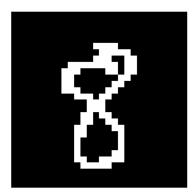
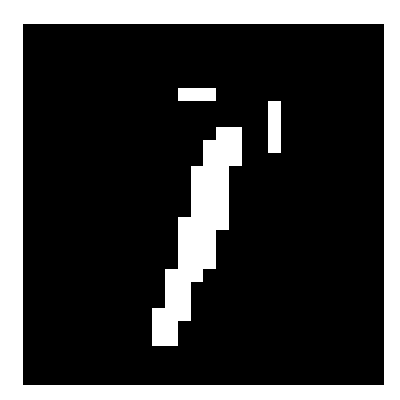
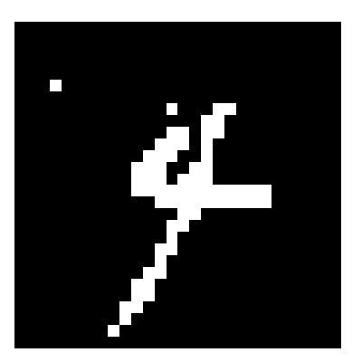
5. Out of curiosity, we treat the black-and-white MNIST digit images as adjacency matrices for directed graphs and see how SCHENO GA modifies the images.

In all of these experiments, the key question is not: can the genetic algorithm can find the optimal result according to SCHENO? for we know that genetic algorithms are limited. Rather, the questions are: does SCHENO reward actual patterns? and how many different kinds of pattern can SCHENO incentivize?

Experiments 2, 3, and 5 are discussed in the appendix. We discuss experiments 1 and 4 in Sections VIII.1 and VIII.2 respectively.

VIII.1 Small, Intuitive Patterns

On small examples, SCHENO GA successfully manages to fill in the gaps and erase the noise in a way that largely corresponds to human intuition. When the result does not correspond to initial expectations, it still makes intuitive sense. See Figure 4 for examples.

(a)

(b)

(c)

(d)

(e)

(f)

Figure 4: Transformations of Small Graphs – The results shown are mostly meant to be intuitive, but some (b and f) took us by surprise, and we leave them here. In the case of (f), our instinct to see human figures blinded us to the actual highly-symmetric structures nearby, structures that SCHENO GA finds.

VIII.2 Real-World Data

SCHENO GA’s most striking results are probably those we obtained on the smaller real-world datasets. We ran SCHENO GA on 6 real-world networks: Zachary’s Karate Club network konect , an ecological food network (what eats what) from Little Rock Lake in Wisconsin konect , a 2004 college football network documenting which FBS teams played at least one game against another team collegefootball , the EU-Core email network snapnets , the Cora ML citation network networkrepository , and a political blogs network showing which blogs reference other blogs konect .

(a) Original Graph

(b) Schema-Noise Decomposition

(c) Schema Only

(d) Noise Only

Figure 5: Performance on the Karate Graph – Note: The node-layouts in the sub-figures are not identical; rather they are arranged individually for visibility. In (b), dark blue represents an original edge, light blue represents an edge SCHENO GA added, and red represents one it deleted.

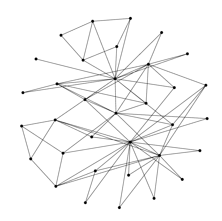
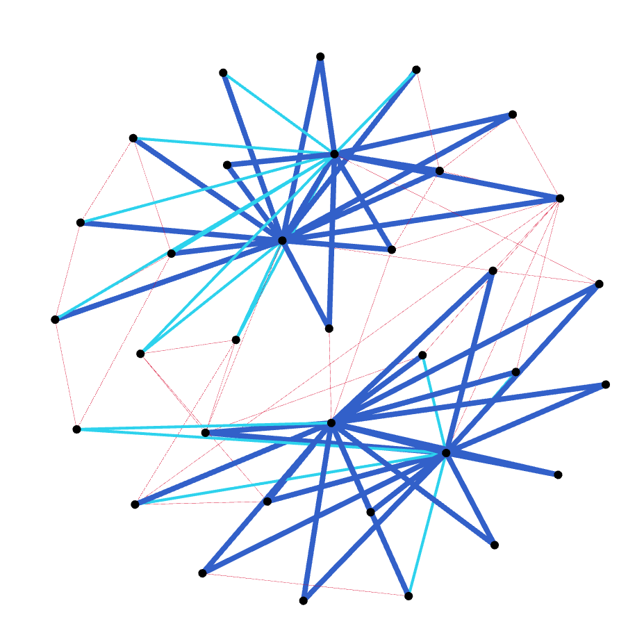
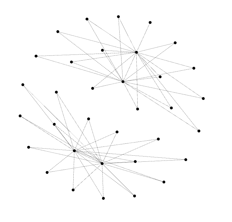
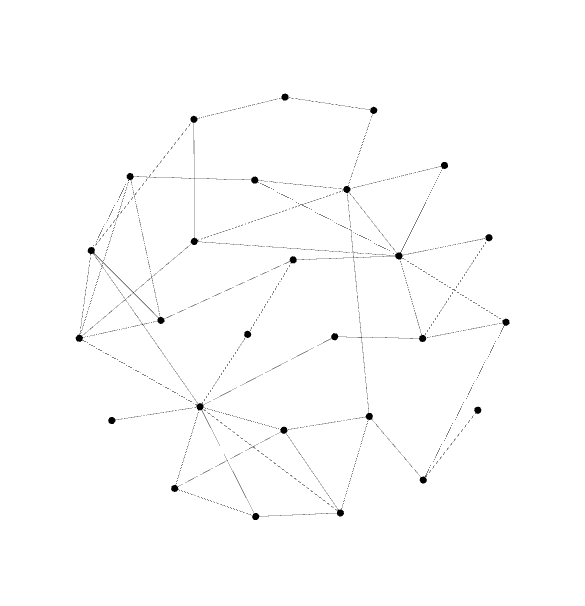
When running on the karate club network, SCHENO GA uncovers the famous historical schism. The network represents social relationships within a club. Eventually the club split into two clubs following two different headmasters. Our algorithm’s decomposition of the graph into schema and noise can be seen in Figure 5. Not only does SCHENO GA notice the split into two groups, but in different trials, our schema decomposition gets between 88 and 94% of the memberships in the eventual historical split correct. Furthermore, we uncover an interesting feature of the graph: For both of the two groups, there is a clear central figure, but there is also a secondary figure that connects to many of the peripheral members of the group.

(a) Edges Added/Removed

(b) Schema Version with Full Symmetries

(c) Edges Added/Removed

(d) Schema Version with Full Symmetries

Figure 6: Performance on the Moreno Foodweb – SCHENO GA finds several anomalous species that eat and/or are eaten by other species in an irregular way. By rectifying these anomalies, the general pattern is restored to the graph. Teal means added; red means deleted.

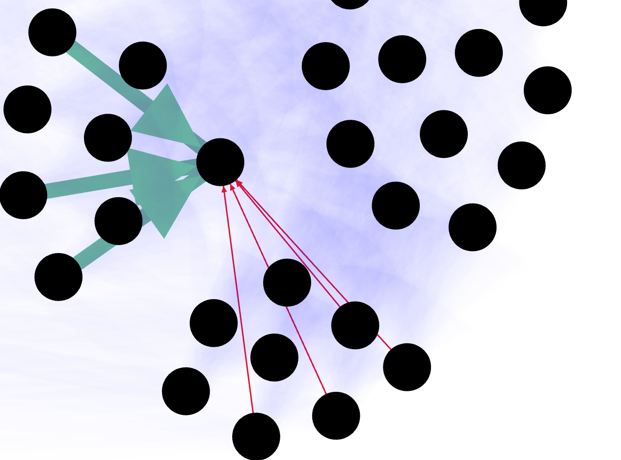
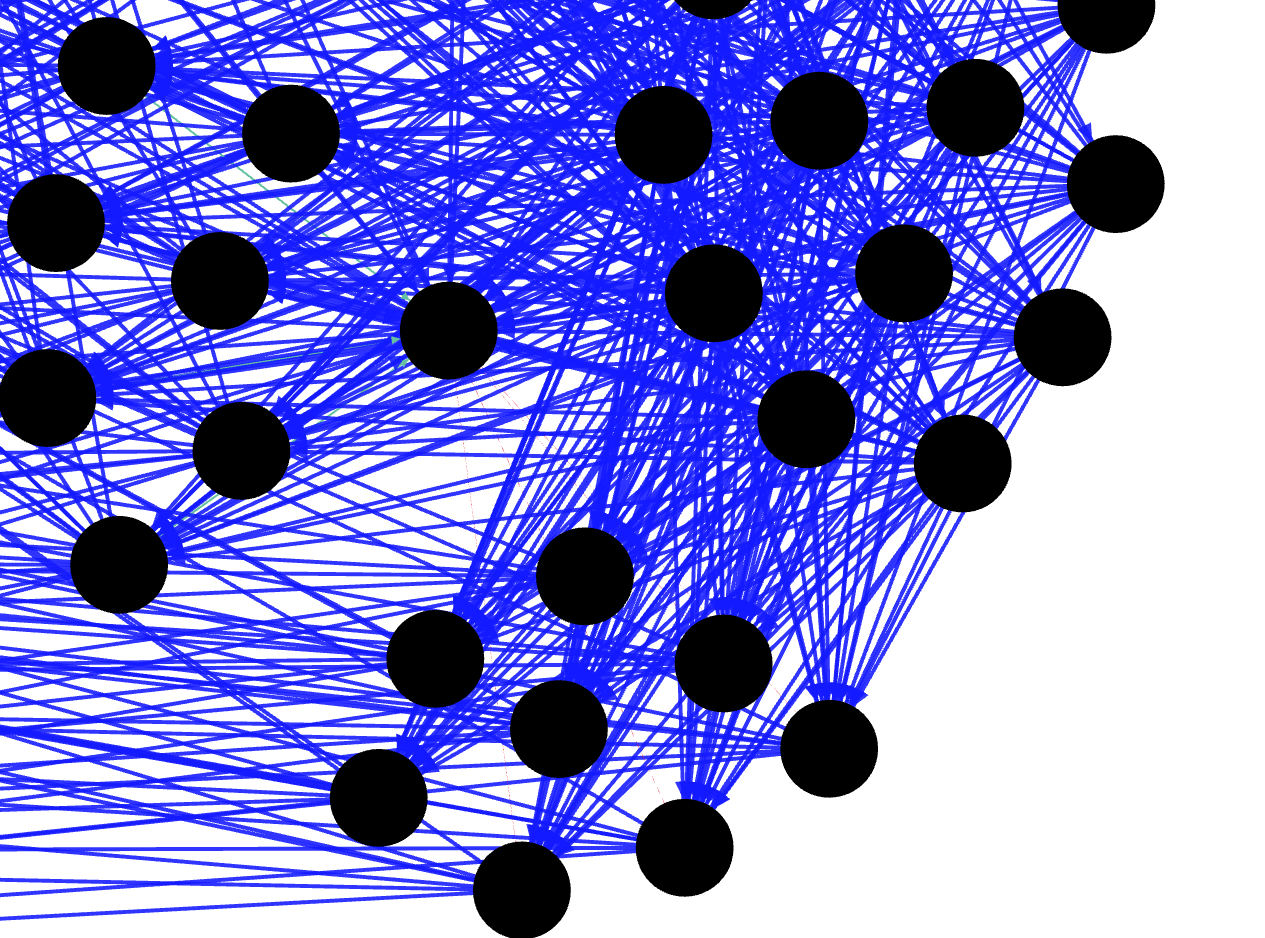
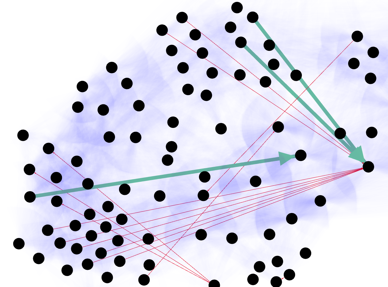
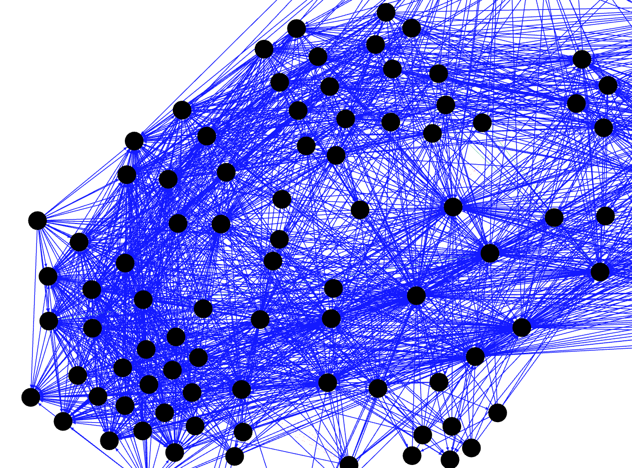
On the ecological food network, SCHENO GA uncovers several anomalies. Broadly speaking, in the network there are groups of species that eat the same things and are eaten by the same things (e.g., a group of bugs that all eat the same plants and are eaten by the same birds). However, anomalies disrupt these symmetries, and our algorithm picks up on this fact. See Figure 6 for illustrations.The results on this graph suggest that in some cases SCHENO-based structure-finding can coincide with anomaly-detection.

(a) Connections Removed

(b) Zoomed-in View of Mostly-FBS Games

Figure 7: Performance on a College Football Graph – The non-FBS teams (aka FCS) get disconnected from the core network.

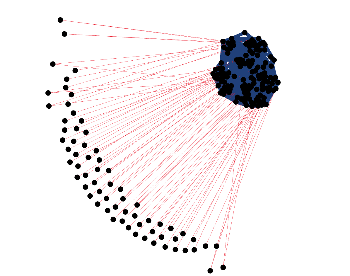
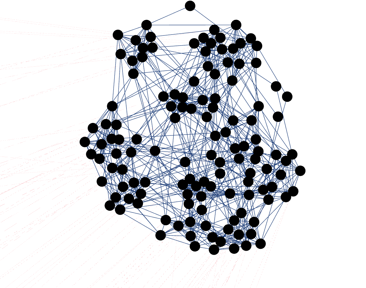
The college football dataset connects two teams if they played at least one game in the 2004 season. The dataset is limited to games with at least one FBS team. SCHENO GA’s one finding was to delete all the edges to non-FBS teams (FCS), treating the schema as the FBS games and the noise as the few edges to FCS teams. This results in a symmetry gain because the newly-disconnected FCS teams all become interchangeable with each other. We think this split makes sense, because from a structural perspective, choosing which FCS team an FBS team plays seems arbitrary. We show the results in Figure 7. We suspect that if SCHENO GA was able to better-explore the search space, it might find further adjustments within the FBS-only games as well, but the relatively greedy process makes no progress on that cluster even though SCHENO might better-reward some other solution.

(a) Some Modifications

(b) Resulting Structure

Figure 8: Performance on Political Blogs Network – The change we highlight here (bottom-right of subfigures) shows the algorithm finding a cluster of nodes that each cite one particular blog and not much else. Again, teal means an edge is added; red means it is deleted.

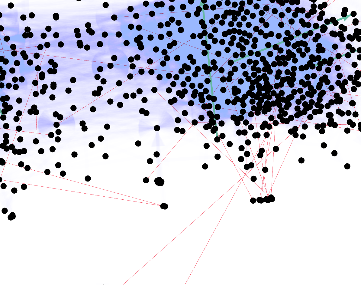
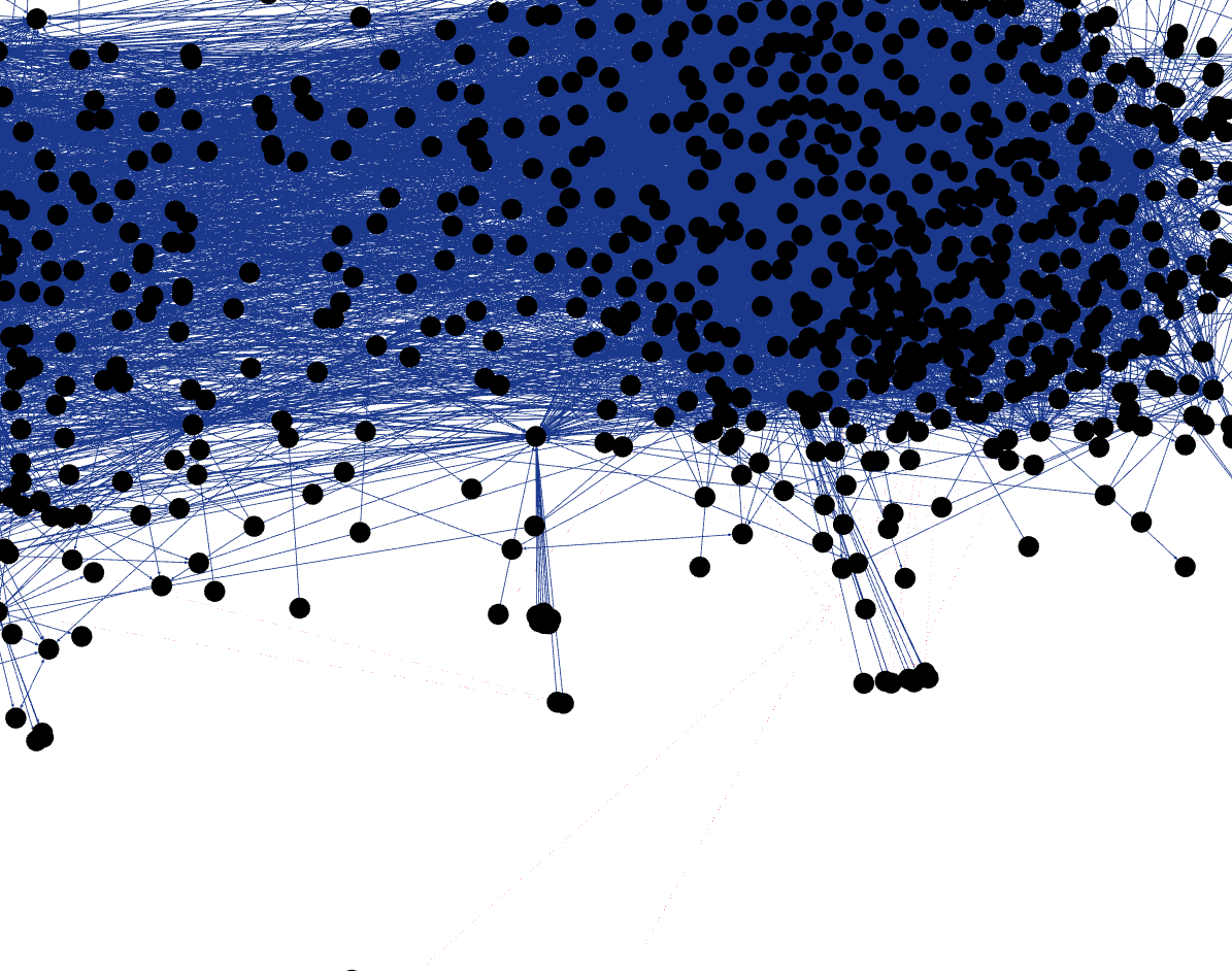
The remaining three graphs, Political Blogs, EU-Core Emails, and Cora Citations receive a few minor adjustments from SCHENO GA, but they are not as interesting. As in the college football graph, our algorithm mostly just deletes connections to nodes with few connections and then leaves a dense and mostly rigid core. There are a few exceptions to this in the political blogs network; we highlight one in Figure 8. As with the football graph, we suspect that this limit on results is due to a lack of power in our search algorithm rather than a lack of power of the SCHENO scoring function, though at the moment we have no certain evidence one way or the other.

In summary, SCHENO GA finds a wide variety of phenomenon across real-world data. The overall trend on real-world data seems to be that the patterns our genetic algorithm can most easily find are those where a group of nodes almost all have identical neighborhoods. Whether or not it is worth making nodes have identical neighborhoods is determined by SCHENO’s specifications for the cost of editing the graph versus the reward of symmetry gains.

IX Concluding Discussion

The SCHENO scoring function offers a principled, goal-agnostic way of measuring how good a job one has done splitting apart a graph into schema and noise. It indicates that some well known graph-mining models have gaps—graphs wherein the patterns they find do not represent the graph’s overall structure and/or do not represent the graph any better than a randomly selected pattern of the same size.

When even a relatively simple process like a genetic algorithm uses SCHENO to produce schema-noise decompositions, we uncover a wide variety of patterns in a wide variety of cases, from intuitive small patterns, to real-world graphs, to combinatoric structures and even image data (see appendix). This demonstrates that SCHENO manages to be a very general metric.

Given the principled origins of our metric, we strongly suspect that with better, more sophisticated search algorithms guided by SCHENO, even more fascinating decompositions can be unearthed on larger and more complex graphs. Another step for future research would be to generalize SCHENO to graphs with node and edge types, or to graphs with weighted edges. Therefore, we expect that these definitions and formulae will likely prove useful to scientists in other fields attempting to uncover new patterns in structured data.

Appendix A More SCHENO GA Results

A.1 Running on Total Noise

As a sanity check, we generate some Erdős-Rényi graphs with edge probability $\frac{1}{2}$, then see what our code finds. We test on 50, 100, 150, and 200 nodes, 3 trials each. As we expected, SCHENO GA does not report a decomposition into structure and noise; it finds nothing, as there is nothing to find.

Technically, this means that SCHENO GA reports that $H=E$ and $N=\emptyset$ (all schema, no noise). We would like this to be reversed, but we expected it is because our genetic algorithm is greedy and would have to delete many edges from $G$ before it would start finding that the whole graph was noise. In absence of finding that the entire graph is noise, we think that finding nothing is best, and that is what SCHENO seems to incentivise.

The more crucial question is: Which decomposition would get a better SCHENO score if the algorithm did manage to find it? This was where we found one surprise: our model’s noise probability $p$ is far enough from the $\frac{1}{2}$ probability we used to generate the noise graphs, that the noise is considered more likely to be structure simply due to the number of edges. This means there is a limit on the applicability of SCHENO: If graphs have many more edges than the proportion of possible edges dictated by our noise probability $p$, even noise might start to look a bit like structure.

Fortunately, this is not much of a problem for SCHENO for four reasons: 1) $p$ gets very close to $\frac{1}{2}$ (e.g. when $n\geq 300$, $p>0.467$). 2) Anyone wishing to extract schema from a graph with over half the possible edges can run on the complement of the graph. 3) People are unlikely to apply SCHENO to random noise, and even less likely to do so on random noise with proportion of edges $>p$. 4) If we generate the Erdős-Rényi graphs using edge probability $p$, then SCHENO correctly says that the entire graph is better explained as noise than as structure (and SCHENO GA still reports to have found nothing).

A.2 Synthetic Structures

Here we considered four combinatoric structures: a 128-node ring, a 127-node balanced binary tree, a 128-node wreath (like a ring, but each node connects to 4 neighbors on each side rather than 1 on each side), and the (10, 3) Johnson graph, which has 120 nodes. An $(a,b)$ Johnson graph has $\binom{a}{b}$ nodes, where each node represents and $a$-size subset of a set of $b$ elements; two nodes are connected if their corresponding sets differ in regard to only one element. Johnson graphs have a high degree of structure, and in fact are fundamentally related to the computational difficulty of the graph isomorphism problem [3].

For each graph, we randomly add and remove a small percentage of edges, then check two things: (1) Would SCHENO incentivise “fixing” the structure? (2) What does SCHENO GA find in practice. These synthetic tests were probably our most lackluster results, but they are still interesting to explore.

Our largest surprise was that the ring and binary tree were too sparse to be considered structure. SCHENO GA effectively said, “There are so few edges that this is basically the empty graph.” The empty graph is not an interesting schema from a human perspective, but it is highly structured in the sense that it has $n!$ automorphisms (each node is interchangeable with any other); in this sense it is equivalent to its complement: the complete graph.

We are not sure at present whether this result is a bug or a feature of SCHENO. On the one hand, the resulting pattern is not particularly fascinating. On the other hand, we tried to define schema in a principled way, and given our conceptual, philosophical setup, this might be the logically “correct” result. Furthermore, SCHENO says that the original synthetic structure is a good schema – much more so than the perturbed graph; SCHENO just says that listing the whole perturbed graph as noise is an even better decomposition.

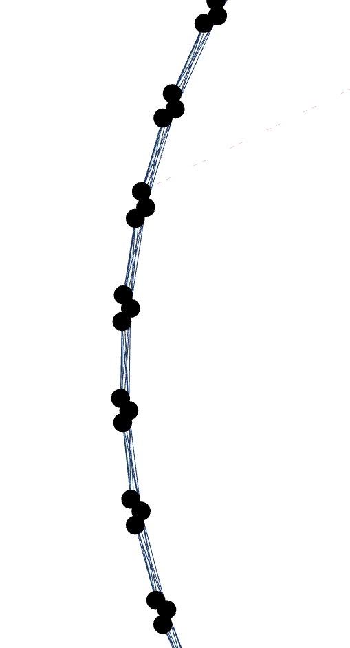
The wreath graph was interesting, because rather than recover the original wreath (modified slightly by noise), SCHENO GA surprised us and pointed out many local symmetries. It found that with a few edits, it could make two or three neighbors in the wreath interchangeable. Thus the algorithm converted the graph into something like a ring lattice. See Figure 9 for some visualizations.

(a) Less Original Noise

(b) More Original Noise

Figure 9: Snapshots of Schema-Noise Decompositions for Randomly-Perturbed Wreath Graphs – Rather than restoring the graph to being a wreath, SCHENO GA instead points out that nodes in a wreath are nearly structurally identical to some of their neighbors; it modifies the structure accordingly to make them actually identical. (a) When less noise is present, the algorithm often makes triples of nodes equivalent to each other. (b) The criss-cross edges were due to the random noise. Here many pairs of nodes are made equivalent; they connect to exactly the same set of nodes.

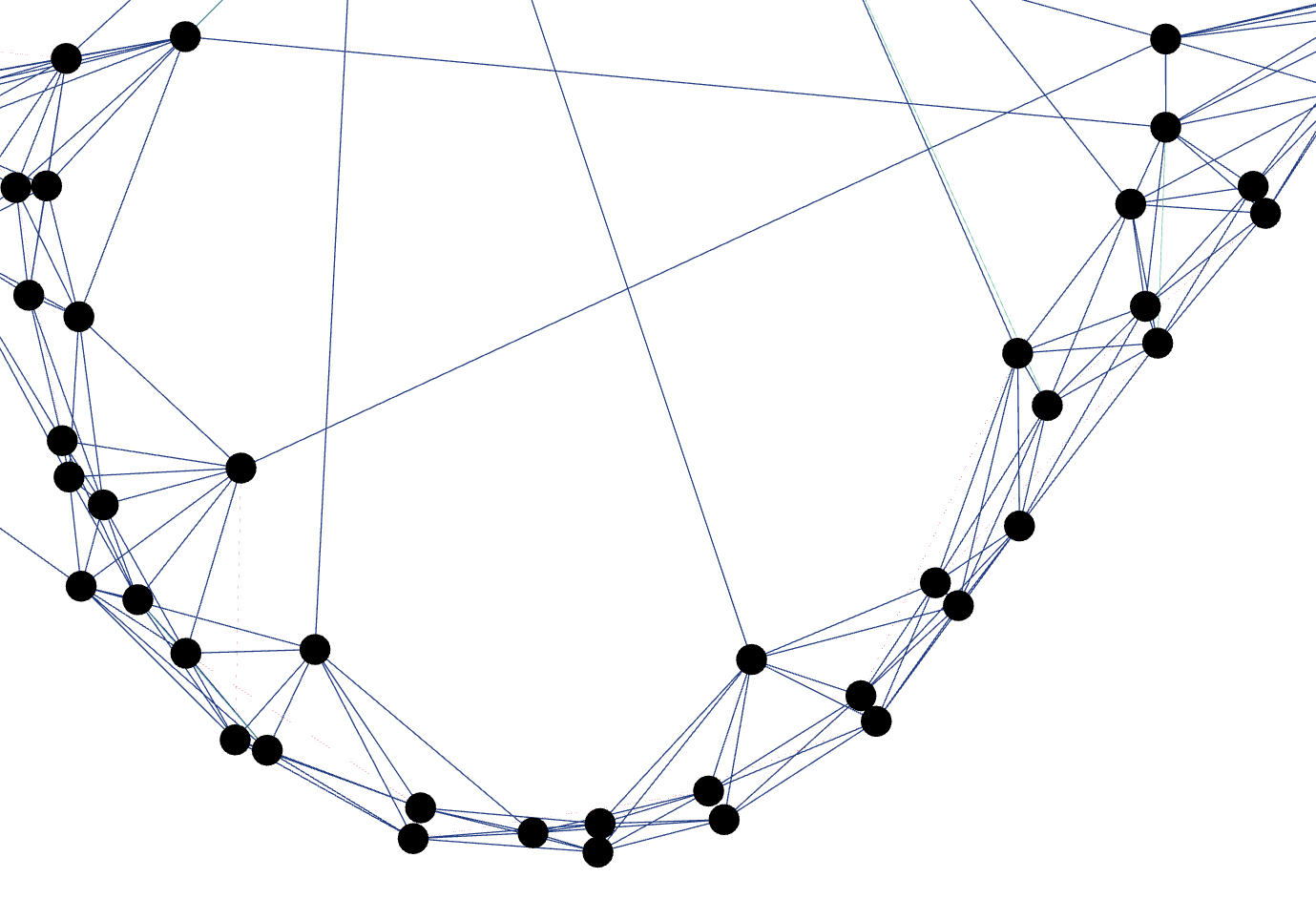
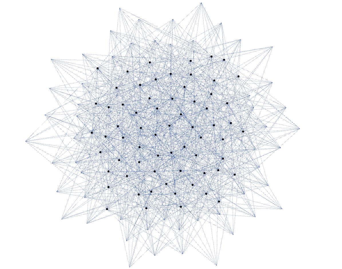
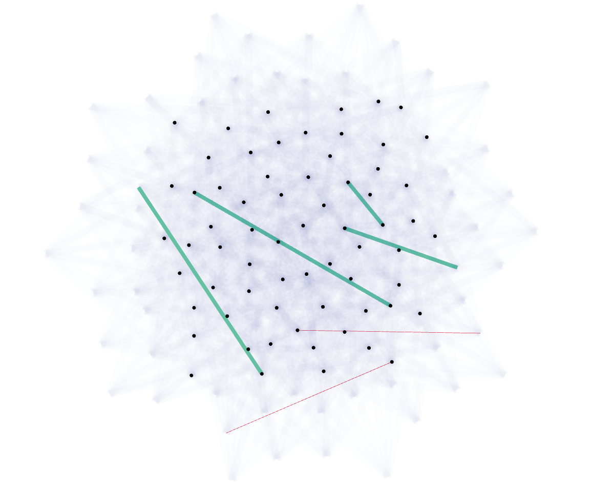
In the Johnson graph, the graph’s symmetries are extremely interrelated to each other, when just a few (e.g. 4 to 5) of the 1,260 edges are randomly perturbed, the graph loses almost all of its symmetry (all of its original 3,628,800 automorphisms). When about 7 or fewer edges are removed, SCHENO GA recovers the structure, but when more are removed, the algorithm struggles. Crucially though, if the genetic algorithm would hypothetically manage to find the noise edges, SCHENO would give the true solution the highest score, but for a genetic algorithm with such a huge search space to explore, this is difficult to find without greedy gains along the way. To get a sense for what the algorithm needs to find we show one of SCHENO GA’s successful runs in Figure 10.

(a) What the Algorithm was Given

(b) What it Found

Figure 10: Performance on the $(10,3)$ Johnson Graph – On the left we see the highly structured form of a Johson graph, but with just 6 incorrect edges, it has only the identity automorphism. The right shows the missing edges as found by SCHENO GA. Teal means that the algorithm added the edges; red means the algorithm deleted them. Once these changes are made, the graph is restored to its 3,628,800 automorphisms.

A.3 MNIST Image Data

We now turn to one final kind of data: images. We look at the MNIST image dataset of black-and-white hand-written digits. An image is not clearly a graph, but we can convert a black-and-white image to a graph by treating the image as an adjacency matrix of a directed graph. As the MNIST digits are white on a black background, we do the conversion as follows:

If pixel $(i,j)$ is white, then we add directed edge $(i,j)$ to the graph when $j<i$, and we add directed edge $(i,j+1)$ to the graph when $j\geq i$. This use of $j+1$ avoids adding self-loops, which our code does not handle at present. To convert back from a graph to an image, we reverse this process; the presence of edge $(i,j)$ means pixel $(i,j)$ is white when $j<i$, and it means pixel $(i,j-1)$ is white when $j>i$.

Overall, we were pleased with the results. We should stress that SCHENO GA is simply trying to find patterns and noise; it is not trying to split handwritten digits into one of the 10 digit categories. As humans we’ve spent our lives learning to identify the relevant “pattern” as “which of the 10 digits is this?” but that is not the only way to see the data. In fact, that is a pattern across images of digits more so than a pattern within an image of a digit, though of course to recognize digits across images, we utilize sub-patterns like lines and curves within an image.

In general, the main trend was to make images more block-like. Sometimes this makes the numeric digits more recognizeable qua digit to a human; sometimes this means finding a different kind of pattern/noise. The key takeaway is that our definition of schema and noise was extremely general and can unearth many kinds of patterns, even in visual data. Our computations were performed on 100 randomly-sampled MNIST digits. We show some representative results in Figures 12, 14, and 16.

(a) Before

(b) After

(c) Before

(d) After

(e) Before

(f) After

(g) Before

(h) After

(i) Before

(j) After

(k) Before

(l) After

(m) Before

(n) After

(o) Before

(p) After

(q) Before

(r) After

(s) Before

(t) After

Figure 12: MNIST – Our Favorite Results

(a) Before

(b) After

(c) Before

(d) After

(e) Before

(f) After

(g) Before

(h) After

(i) Before

(j) After

(k) Before

(l) After

(m) Before

(n) After

(o) Before

(p) After

(q) Before

(r) After

(s) Before

(t) After

Figure 14: MNIST – Typical Results

(a) Before

(b) After

(c) Before

(d) After

(e) Before

(f) After

(g) Before

(h) After

(i) Before

(j) After

(k) Before

(l) After

(m) Before

(n) After

(o) Before

(p) After

(q) Before

(r) After

(s) Before

(t) After

Figure 16: MNIST – Strangest Results – The tendency to “blockify” continues. Some images with few white pixels are made even sparser. The changes we least understand are the last two shown.

References

- [1] schema, n. In OED Online. Oxford University Press, 2024.
- [2] Fred Attneave. Some informational aspects of visual perception. Psychological review, 61(3):183, 1954.
- [3] László Babai. Graph isomorphism in quasipolynomial time. In Proceedings of the forty-eighth annual ACM symposium on Theory of Computing, pages 684–697, 2016.
- [4] Fabian Ball and Andreas Geyer-Schulz. How symmetric are real-world graphs? a large-scale study. Symmetry, 10(1):29, 2018.
- [5] Béla Bollobás. Random graphs. Springer, 1998.
- [6] CFBD. Collegefootballdata.com. https://collegefootballdata.com/exporter/, July 2023.
- [7] Susan F Chipman. Complexity and structure in visual patterns. Journal of Experimental Psychology: General, 106(3):269, 1977.
- [8] Yongwook Choi and Wojciech Szpankowski. Compression of graphical structures: Fundamental limits, algorithms, and experiments. IEEE Transactions on Information Theory, 58(2):620–638, 2012.
- [9] Jonathan Cohen. Trusses: Cohesive subgraphs for social network analysis. National security agency technical report, 16(3.1):1–29, 2008.
- [10] Diane J Cook and Lawrence B Holder. Substructure discovery using minimum description length and background knowledge. Journal of Artificial Intelligence Research, 1:231–255, 1993.
- [11] Matthias Dehmer and Abbe Mowshowitz. Inequalities for entropy-based measures of network information content. Applied Mathematics and Computation, 215(12):4263–4271, 2010.
- [12] Matthias Dehmer and Abbe Mowshowitz. Generalized graph entropies. Complexity, 17(2):45–50, 2011.
- [13] Maria Fox, Derek Long, and Julie Porteous. Discovering near symmetry in graphs. In PROCEEDINGS OF THE NATIONAL CONFERENCE ON ARTIFICIAL INTELLIGENCE, volume 22, page 415. Menlo Park, CA; Cambridge, MA; London; AAAI Press; MIT Press; 1999, 2007.
- [14] Frank Harary and Edgar M Palmer. Graphical enumeration. Elsevier, 2014.
- [15] Justus Isaiah Hibshman. Ratio of symmetries between any two n-node graphs. arXiv preprint arXiv:2205.05726, 2022.
- [16] Julian Hochberg and Edward McAlister. A quantitative approach, to figural” goodness”. Journal of Experimental Psychology, 46(5):361, 1953.
- [17] Ben Knueven, Jim Ostrowski, and Sebastian Pokutta. Detecting almost symmetries of graphs. Mathematical Programming Computation, 10:143–185, 2018.
- [18] Danai Koutra, U Kang, Jilles Vreeken, and Christos Faloutsos. Vog: Summarizing and understanding large graphs. In Proceedings of the 2014 SIAM international conference on data mining, pages 91–99. SIAM, 2014.
- [19] Jérôme Kunegis. KONECT – The Koblenz Network Collection. In Proc. Int. Conf. on World Wide Web Companion, pages 1343–1350, 2013.
- [20] Jure Leskovec and Andrej Krevl. SNAP Datasets: Stanford large network dataset collection. http://snap.stanford.edu/data, June 2014.
- [21] Angsheng Li and Yicheng Pan. Structural information and dynamical complexity of networks. IEEE Transactions on Information Theory, 62(6):3290–3339, 2016.
- [22] Gregory R Lockhead and James R Pomerantz. The perception of structure: Essays in honor of Wendell R. Garner. American Psychological Association, 1991.
- [23] Ben D MacArthur, Rubén J Sánchez-García, and James W Anderson. Symmetry in complex networks. Discrete Applied Mathematics, 156(18):3525–3531, 2008.
- [24] I Markov. Almost-symmetries of graphs. In Proc. International Symmetry Conference (ISC), pages 60–70, 2007.
- [25] Igor L Markov. Algebraic structure helps in finding and using almost-symmetries.
- [26] Brendan D McKay and Adolfo Piperno. Practical graph isomorphism, ii. Journal of symbolic computation, 60:94–112, 2014.
- [27] Abbe Mowshowitz and Matthias Dehmer. Entropy and the complexity of graphs revisited. Entropy, 14(3):559–570, 2012.
- [28] Here is analogous to the XOR function.
- [29] Stephen E Palmer. Goodness, gestalt, groups, and garner: Local symmetry subgroups as a theory of figural goodness. 1991.
- [30] Stephen E Palmer and Kathleen Hemenway. Orientation and symmetry: effects of multiple, rotational, and near symmetries. Journal of Experimental Psychology: Human Perception and Performance, 4(4):691, 1978.
- [31] Federica Parisi, Guido Caldarelli, and Tiziano Squartini. Entropy-based approach to missing-links prediction. Applied Network Science, 3(1):1–15, 2018.
- [32] Julie Porteous, Derek Long, and Maria Fox. The identification and exploitation of almost symmetries in planning problems. In Proceedings of the 23rd Workshop of the UK Planning and Scheduling Special Interest Group, pages 130–136, 2004.
- [33] HE Rose. Action and the orbit–stabiliser theorem. A Course on Finite Groups, pages 91–111, 2009.
- [34] Ryan Rossi and Nesreen Ahmed. The network data repository with interactive graph analytics and visualization. In Twenty-ninth AAAI conference on artificial intelligence, 2015.
- [35] Fred L Royer. Detection of symmetry. Journal of Experimental Psychology: Human Perception and Performance, 7(6):1186, 1981.
- [36] Claude Elwood Shannon. A mathematical theory of communication. The Bell system technical journal, 27(3):379–423, 1948.
- [37] Satyaki Sikdar, Justus Hibshman, and Tim Weninger. Modeling graphs with vertex replacement grammars. In 2019 IEEE International Conference on Data Mining (ICDM), pages 558–567. IEEE, 2019.
- [38] Tao Wen and Wen Jiang. Measuring the complexity of complex network by tsallis entropy. Physica A: Statistical Mechanics and its Applications, 526:121054, 2019.
- [39] Yang-Hua Xiao, Wen-Tao Wu, Hui Wang, Momiao Xiong, and Wei Wang. Symmetry-based structure entropy of complex networks. Physica A: Statistical Mechanics and its Applications, 387(11):2611–2619, 2008.
- [40] Zhongqi Xu, Cunlai Pu, Rajput Ramiz Sharafat, Lunbo Li, and Jian Yang. Entropy-based link prediction in weighted networks. Chinese Physics B, 26(1):018902, 2017.
- [41] Likang Yin, Haoyang Zheng, Tian Bian, and Yong Deng. An evidential link prediction method and link predictability based on shannon entropy. Physica A: Statistical Mechanics and its Applications, 482:699–712, 2017.