Spontaneous emission decay and excitation in photonic temporal crystals

Abstract

Over the last few decades, the prominent strategies for controlling spontaneous emission has been the use of resonant or space-periodic photonic structures [1, 2, 3, 4, 5, 6, 7, 8, 9, 10, 11, 12, 13, 14, 15, 16]. This approach, initially articulated by Purcell [17] and later expanded upon by Yablonovitch in the context of photonic crystals [1], leverages the spatial surroundings to modify the spontaneous emission decay rate of atoms or quantum emitters. However, the rise of time-varying photonics [18, 19, 20, 21, 22, 23, 24, 25, 26, 27, 28, 29, 30] has compelled a reevaluation of the spontaneous emission process within dynamically changing environments, especially concerning photonic temporal crystals where optical properties undergo time-periodic modulation [18, 20]. Here, we apply classical light-matter interaction theory along with Floquet analysis to reveal a substantial enhancement in the spontaneous emission decay rate at the momentum gap frequency in photonic temporal crystals. This enhancement is attributed to time-periodicity-induced loss and gain mechanisms, as well as the non-orthogonality of Floquet eigenstates that are inherent to photonic temporal crystals. Intriguingly, our findings also suggest that photonic temporal crystals enable the spontaneous excitation of an atom from its ground state to an excited state, accompanied by the concurrent emission of a photon.

The investigation into electromagnetic wave dynamics within space-time periodic media began in the 1960s, aiming to elucidate the temporally-growing instabilities in distributed parametric media [31, 32]. The field of time-varying photonics, however, did not draw widespread attention until an experiment using a time-periodic transmission line unveiled a shallow, yet definitive, momentum gap [33]. This experimental finding spurred the conceptual expansion of photonic spatial crystals and metamaterial principles into the space-time domain. More specifically, the enhanced dispersion and band structure engineering capabilities made possible by the extra temporal degree of freedom have been the subject of the most thorough research [21, 22, 23, 24, 25]. This advancement in time-varying photonics has further paved the way for exploring a multitude of intriguing phenomena, including colossal broadband nonreciprocity [19], efficient one-way amplification [23], parametric oscillation [28, 27], pulse compression [34], harmonic generation [22], and even the mimicry of Hawking radiation [35], all of which are now being explored for their potential applications.

Only recently, however, has the Floquet systems analysis been used to shed more light on our understanding of photonic temporal crystals (PTCs) [20]. The effective Hamiltonian matrix for PTCs, derived from Maxwell’s equations, is identified as pseudo-Hermitian. Consequently, this leads to the photonic Floquet eigenstates becoming non-orthogonal. Furthermore, the momentum gap is proven to be the pseudo-Hermiticity broken phase along the wavenumber axis, while its edges are identified as non-Hermitian degeneracies, i.e., exceptional points (EPs) [20, 27]. These findings highlight the need for a non-Hermitian theoretical framework to analyze the phenomena associated with PTCs. Moreover, in the context of light-matter interactions, the analytical complexities and subtleties associated with non-Hermitian dynamics within PTCs become particularly evident. Taking these non-Hermitian dynamics into account, we demonstrate below that the spontaneous emission (SE) decay rate at the edge of momentum gaps in PTCs is markedly enhanced. This finding sharply contradicts a recent publication [26], which predicted the complete vanishing of SE decay at the momentum gap frequency.

For precise quantification of light-matter interactions in PTCs, we first need to consider the fact that PTCs exhibit time-periodicity-induced loss and gain regions in wavenumber-frequency space, each of which is manifested by positive or negative (partial) momentum-resolved density of states ($\mathrm{kDOS}$). The negative $\mathrm{kDOS}$ within the gain region necessitates a gain-induced correction, thereby necessitating a reevaluation of the SE decay rate [36, 37, 38, 39, 40]. More intriguingly, the presence of gain in PTCs imply a spontaneous excitation of an atom from its ground to the excited state, accompanied by the emission of a photon, suggesting more diversified light-matter interactions in non-equilibrium photonic settings. Finally, in addition to highlighting the significance of time-periodicity-induced loss and gain, we draw attention to the role played by the non-orthogonality of photonic Floquet eigenstates, characterized by the Petermann factor ($\mathrm{PF}$), in enhancing the SE decay and excitation rates [41, 42, 43, 44].

Electrodynamics within PTCs can be investigated by solving Maxwell’s equations for a medium characterized by time-periodic relative permittivity, $\epsilon(t)=\epsilon(t+2\pi/\Omega)$, where $\Omega$ denotes the (angular) frequency of time-periodic modulation (Fig. 1a):

$$\nabla\times\mathbf{E}(\mathbf{r},t) =-\mu\frac{\partial}{\partial t}\mathbf{H}(\mathbf{r},t),$$ (1)

$$\nabla\times\mathbf{H}(\mathbf{r},t) =\frac{\partial}{\partial t}[\epsilon(t)\mathbf{E}(\mathbf{r},t)]+\mathbf{J}(\mathbf{r},t)+\sigma\mathbf{E}(\mathbf{r},t).$$ (2)

Due to the time-periodicity, the relative permittivity $\epsilon(t)$ can be expanded as $\epsilon(t)=\sum_{n}\epsilon_{n}e^{-in\Omega t}$, where $n$ spans all integers. For the sake of mathematical simplicity, both the vacuum permittivity and permeability are set to 1, i.e., $\epsilon_{v}=\mu_{v}=1$. The conductivity $\sigma$ is introduced to explore the impact of intrinsic losses ($\sigma>0$) on light-matter interactions, although consideration of other loss models is also possible [20].

Figure 1: (a) Schematic rendering of time-periodic permittivity variation. (b) Illustration of the Floquet band structure of a PTC, characterized by a sinusoidally-modulated relative permittivity $\epsilon(t)=\epsilon_{0}+\epsilon_{m}\sin{\Omega t}$. Here, the band structure is plotted using the following parameters: $\epsilon_{0}=5$, $\epsilon_{m}=1.5$, $\mu=1$, and $\Omega=1$. The plots correspond to the case where the conductivity is set to the critical value $\sigma=\sigma_{c}=0.3715$. The momentum gap (MG) is highlighted in yellow.

Figure 2: (a) Map of $\mathrm{kDOS}$ and the SE decay rate $\Gamma$ for $\sigma=0.4>\sigma_{c}$ (large loss case). (b, c) Plot of $\rho_{\mathbf{p}}(\mathbf{k},\omega)$ and its decompositions, shown as a function of frequency for $k=0.9$ (outside the momentum gap) and 1.05 (within the central gap region). The $\mathrm{kDOS}$ outside the gap is approximated by a sum of two scaled Lorentzian lineshape functions with opposite signs, whereas the $\mathrm{kDOS}$ within the gap exhibits a non-Lorentzian character. These plots highlight the positive-valued $\mathrm{kDOS}$ across the entire $(\mathbf{k},\omega)$ space in the case of large loss. (d) Map of $\mathrm{kDOS}$, with plots of SE decay and excitation rates for $\sigma=0.1<\sigma_{c}$ (small loss case). (e, f) Plot of $\rho_{\mathbf{p}}(\mathbf{k},\omega)$ and its decompositions, shown as a function of frequency for $k=0.9$ (outside the gap) and 1.05 (within the central gap region). The decomposition conducted outside the gap reveals a negative $\mathrm{kDOS}$ near the Floquet sideband of the negative frequency band. These plots were generated under the assumption that $\mathbf{k}$ is perpendicular to $\mathbf{n}_{\mathbf{p}}$, except for the calculations of the SE decay and excitation rates. For comparison, the SE decay rate in a homogeneous, time-invariant medium, characterized by a relative permittivity of $\epsilon_{0}$, is also plotted with a black dashed line in the left panels of (a) and (d).

In classical light-matter interaction theory, a two-level atom is modeled as an oscillating point electric dipole, $\mathbf{p}(\mathbf{r},t)=\mathrm{Re}[\mathbf{p}\delta(\mathbf{r}-\mathbf{r}_{0})\exp(-i\omega t)]$, simplifying the complex scenarios into a more comprehensible classical framework [45]. It is also noteworthy that the SE decay rate in the weak coupling regime can be estimated from purely classical power flow (or radiation reaction) arguments, even in linearly amplifying media, illustrating quantum-classical correspondence [36, 37, 38]. With this in mind, we incorporate the dipole-induced current source, $\mathbf{J}=\partial\mathbf{p}/\partial t$, into the Maxwell equations for the PTC. The Floquet analysis, along with the power flow analysis, leads to the (partial) momentum-resolved photonic density of states ($\mathrm{kDOS}$), $\rho_{\mathbf{p}}(\mathbf{k},\omega)$, expressed as,

$$\rho_{\mathbf{p}}(\mathbf{k},\omega)\equiv\frac{2\epsilon_{0}\mu\omega}{\pi}\mathrm{Im}[\mathbf{n}_{\mathbf{p}}\cdot\mathbb{G}_{0}(\mathbf{k},\omega)\cdot\mathbf{n}_{\mathbf{p}}],$$ (3)

where $\mathbb{G}_{0}(\mathbf{k},\omega)$ is the dyadic Green’s function, defined as $\mathbb{G}_{0}(\mathbf{k},\omega)\equiv\mathbb{G}(\mathbf{k},\omega,\omega)=-(\mu\omega)^{-1}\delta_{0}\cdot\mathcal{G}_{F}(\mathbf{k},\omega)\cdot A_{F}\otimes\mathbb{I}$, $\delta_{0}$ is a matrix that extracts the electric field component at $\omega$, $A_{F}$ is a column vector that contains the time-periodic permittivity information, $\mathbb{I}$ is the unit dyad, $\mathcal{G}_{F}(\mathbf{k},\omega)$ is the Green’s function, given as $\mathcal{G}_{F}(\mathbf{k},\omega)=[\omega\mathbf{I}_{F}-\mathcal{H}_{F}(\mathbf{k})]^{-1}$, $\mathbf{I}_{F}$ is the identity matrix with the same size as $\mathcal{H}_{F}(\mathbf{k})$, and $\mathbf{n}_{\mathbf{p}}$ is the unit vector in the direction of the dipole (see supplementary information A). The non-Hermitian Floquet Hamiltonian matrix, $\mathcal{H}_{F}$, is derived from Maxwell’s equations and is also given in the supplementary information A. The Green’s function is expressible using the left and right Floquet eigenvectors, $\bra{L_{m}(\mathbf{k})}$ and $\ket{R_{m}(\mathbf{k})}$ [46, 47]:

$$\mathcal{G}_{F}(\mathbf{k},\omega)=\sum_{m}\frac{1}{\omega-\omega_{m}(\mathbf{k})}\frac{\ket{R_{m}(\mathbf{k})}\bra{L_{m}(\mathbf{k})}}{\innerproduct{L_{m}(\mathbf{k})}{R_{m}(\mathbf{k})}},$$ (4)

where the integer $m$ represents the mode index, and $\omega_{m}=\Omega_{m}-i\gamma_{m}$ is the complex-valued quasi-eigenfrequency. The time-averaged, momentum-resolved power, $\bar{P}(\mathbf{k},\omega)$, dissipated by an extended dipole, is found to be proportional to the $\mathrm{kDOS}$ (see supplementary information B):

$$\bar{P}(\mathbf{k},\omega) =\frac{1}{(2\pi)^{3}}\frac{\omega^{3}\mu|\mathbf{p}|^{2}}{2}\mathrm{Im}[\mathbf{n}_{\mathbf{p}}\cdot\mathbb{G}_{0}(\mathbf{k},\omega)\cdot\mathbf{n}_{\mathbf{p}}]$$ (5)

$$=\frac{1}{(2\pi)^{3}}\frac{\pi\omega^{2}|\mathbf{p}|^{2}}{4\epsilon_{0}}\rho_{\mathbf{p}}(\mathbf{k},\omega).$$

To proceed further, we plot the Floquet band structure in Fig. 1b, revealing the presence of the momentum gap. We assume a sinusoidal permittivity variation without loss of generality, with a modulation depth of $\epsilon_{m}/\epsilon_{0}=0.3$. This allows the conductivity $\sigma$ to solely determine the maximum value of the bifurcated imaginary parts of eigenfrequencies, denoted as $\gamma_{\mathrm{max}}$, within the momentum gap. It can also be proven that the EPs persist even in the presence of the conductivity $\sigma$, rendering a constant imaginary part of the eigenfrequencies outside the momentum gap (see supplementary information C). By defining the critical conductivity $\sigma_{c}$ as the value at which $\gamma_{\mathrm{max}}$ reaches zero, we can identify two distinct regimes of interest: (i) the large intrinsic loss regime, and (ii) the small intrinsic loss regime.

Let us first investigate the case of large intrinsic loss, where $\sigma>\sigma_{c}$ (or $\gamma_{\mathrm{max}}<0$). The time-averaged power dissipated by an oscillating point electric dipole can be calculated by integrating $\bar{P}(\mathbf{k},\omega)$ over the entire wavenumber space,

$$\bar{P}(\omega)=\frac{1}{(2\pi)^{3}}\frac{\pi\omega^{2}|\mathbf{p}|^{2}}{4\epsilon_{0}}\int_{\mathbb{K}}\rho_{\mathbf{p}}(\mathbf{k},\omega)d^{3}\mathbf{k}.$$ (6)

To quantify the SE decay rate, one must first calculate the Purcell factor, given by $\mathrm{F}(\omega)=\bar{P}(\omega)/P_{0}(\omega)$, where $P_{0}$ represents the power radiated by an oscillating point electric dipole in a vacuum. Then, the SE decay rate can be calculated by $\Gamma(\omega)=\Gamma_{0}(\omega)\mathrm{F}(\omega)=\pi\omega(\hbar\epsilon_{0})^{-1}|\mathbf{\tilde{p}}|^{2}(2\pi)^{-3}\int_{\mathbb{K}}{\rho_{\mathbf{p}}(\mathbf{k},\omega)\ d^{3}\mathbf{k}}$, where $\Gamma_{0}$ represents the SE decay rate in a vacuum and $\mathbf{\tilde{p}}=\bra{g}\hat{\bm{\mathbf{p}}}\ket{e}$ denotes the transition dipole matrix element.

If we consider only the two bands ($\omega_{+}=\Omega_{+}-i\gamma_{+}$ and $\omega_{-}=\Omega_{-}-i\gamma_{-}$) that contribute to the formation of the momentum gap at $\omega=\Omega/2$, we can approximate the $\mathrm{kDOS}$ as follows, provided that $\mathbf{k}$ is perpendicular to $\mathbf{n}_{\mathbf{p}}$ (see supplementary information B for the case where $\mathbf{k}$ is parallel to $\mathbf{n}_{\mathbf{p}}$):

$$\rho_{\mathbf{p}}(\mathbf{k},\omega) \approx\sum_{\alpha=\pm}\rho_{\mathbf{p}}^{\alpha}(\mathbf{k},\omega)$$ (7)

$$\approx\sum_{\alpha=\pm}\frac{1}{\pi}\frac{\gamma_{\alpha}}{(\omega-\Omega_{\alpha})^{2}+\gamma_{\alpha}^{2}}\mathrm{Re}[I_{\alpha}(\mathbf{k})]$$

$$\qquad\,+\frac{1}{\pi}\frac{\Omega_{\alpha}-\omega}{(\omega-\Omega_{\alpha})^{2}+\gamma_{\alpha}^{2}}\mathrm{Im}[I_{\alpha}(\mathbf{k})],$$

where $I_{\alpha}(\mathbf{k})$ is expressed as

$$I_{\alpha}(\mathbf{k})=\mathbf{n}_{\mathbf{p}}\cdot\left[2\delta_{0}\cdot\frac{\ket{R_{\alpha}(\mathbf{k})}\bra{L_{\alpha}(\mathbf{k})}}{\innerproduct{L_{\alpha}(\mathbf{k})}{R_{\alpha}(\mathbf{k})}}\cdot\epsilon_{0}A_{F}\otimes\mathbb{I}\right]\cdot\mathbf{n}_{\mathbf{p}}.$$ (8)

Outside the momentum gap, the imaginary part of $I_{\alpha}(\mathbf{k})$ is negligible while the real part is significant; additionally, the real part of $I_{+}(\mathbf{k})$ exhibits a positive sign, whereas that of $I_{-}(\mathbf{k})$ displays a negative sign. Consequently, when the wavenumber is fixed (outside the gap), the $\mathrm{kDOS}$ is approximated by a sum of two scaled Lorentzian lineshape functions with opposite signs. Each Lorentzian lineshape function is scaled by the real part of $I_{\alpha}(\mathbf{k})$, whose magnitude sharply increases as the wavenumber nears the edge of the gap. In PTCs, specifically outside the gap, the role traditionally played by the normalized (projected) electric field intensity in Hermitian photonic systems is now assumed by the real part of $I_{\alpha}(\mathbf{k})$, reflecting the non-Hermitian characteristics of these systems. In the time-invariant limit ($\epsilon_{m}\rightarrow 0$), it can also be shown that $\rho_{\mathbf{p}}^{-}(\mathbf{k},\omega)$ approaches zero, thereby simplifying the $\mathrm{kDOS}$ to that of the time-invariant medium.

In Fig. 2a, the $\mathrm{kDOS}$ map is plotted, clearly showing that $\mathrm{kDOS}$ exhibits net positive values across the entire $(\mathbf{k},\omega)$ space. Figures 2b and 2c illustrate the $\mathrm{kDOS}$ and its decompositions at specific $k$ values: $k=0.9$ (outside the gap) and $k=1.05$ (within the central gap region), respectively. The $\mathrm{kDOS}$ outside the gap reaches its minimum, yet retains a positive value, near the Floquet sideband of the negative frequency band (Fig. 2b). Within the central gap region, it is evident that the imaginary part of $I_{\alpha}(\mathbf{k})$ is no longer negligible, resulting in a significant deviation of $\rho_{\mathbf{p}}^{\alpha}(\mathbf{k},\omega)$ from a Lorentzian lineshape function (Fig. 2c). In this case of large intrinsic loss, the $\mathrm{kDOS}$ spontaneous emission model remains valid and can be reliably applied [47, 48]. This model predicts an enhanced, yet finite, SE decay rate near the momentum gap frequency (see the left panel of Fig. 2a). For comparison, the SE decay rate in a homogeneous, time-invariant medium, characterized by a relative permittivity of $\epsilon_{0}$, is also plotted with a black dashed line.

Now, let us delve into the more subtle case of small intrinsic loss, characterized by $\sigma<\sigma_{c}$ or $\gamma_{\mathrm{max}}>0$. In such cases, the $\mathrm{kDOS}$ outside the gap becomes negative near the Floquet sideband of the negative frequency band, as illustrated in Figs. 2d and 2e. Notably, this negativity extends into the central gap region, as depicted in Figs. 2d and 2f. The concept of negative local density of states has been explored in the context of spontaneous emission in linear amplifying media [38, 39], as well as in the spectral functions of driven, dissipative, nonlinear quantum systems [40]. The negative $\mathrm{kDOS}$ in our case is uniquely attributed to the net gain arising from time-periodic modulation of permittivity. In the supplementary information D, we show that consistent results can be obtained by adopting a driven Lorentz oscillator model with a time-periodic elastic constant. To accurately determine the SE decay rate in such cases, it is necessary to define a corrected Purcell factor that only considers the regions with positive $\mathrm{kDOS}$ values [38, 37]. This corrected Purcell factor, $\mathrm{F}_{l}(\omega)=\bar{P}_{l}(\omega)/P_{0}(\omega)$, where $\bar{P}_{l}(\omega)$ is the power dissipated by the dipole, can be determined by integrating $\rho_{\mathbf{p}}(\mathbf{k},\omega)$ over the lossy region $\mathbb{K}_{l}$, where $\rho_{\mathbf{p}}(\mathbf{k},\omega)>0$, $\forall\mathbf{k}\in\mathbb{K}_{l}$: $\bar{P}_{l}(\omega)=(2\pi)^{-3}\pi\omega^{2}|\mathbf{p}|^{2}/(4\epsilon_{0})\int_{\mathbb{K}_{l}}\rho_{\mathbf{p}}(\mathbf{k},\omega)d^{3}\mathbf{k}$. Then, the corrected SE decay rate can be expressed as $\Gamma_{l}(\omega)=\Gamma_{0}(\omega)\mathrm{F}_{l}(\omega)$.

Figure 3: (a) Two types of points identified at the momentum gap frequency: EPs located at $k_{EP_{-}}$ and $k_{EP_{+}}$, and simple poles at $k_{R_{-}}$ and $k_{R_{+}}$ (indicated by the symbols $\circ$ ). The blue regions indicate areas associated with decay, whereas the red regions denote areas linked to excitation. (b) Trajectories of two singular points in the complex wavenumber plane as a function of frequency variation, demonstrating the transition from simple poles to branch point singularities upon detuning from the momentum gap frequency. Here, the symbols $\circ$ and $\times$ indicate the simple pole and the branch point singularity, respectively.

When interpreted within a quantum framework, the observation of negative $\mathrm{kDOS}$ implies a spontaneous transition of a two-level atom from its ground state to an excited state [36], accompanied by the emission of a photon, i.e., $\ket{g,0}$ to $\ket{e,1}$. This process is spontaneous in the sense that it is mediated not by a photon but by quantum pumping due to the gain induced by time-periodicity. The corresponding SE excitation rate is expressed as $\Gamma_{g}(\omega)=\Gamma_{0}(\omega)\bar{P}_{g}(\omega)/P_{0}(\omega)$, where the power flow into the point dipole can be determined by integrating the absolute value of $\rho_{\mathbf{p}}(\mathbf{k},\omega)$ over the gain region $\mathbb{K}_{g}$, where $\rho_{\mathbf{p}}(\mathbf{k},\omega_{0})<0$, $\forall\mathbf{k}\in\mathbb{K}_{g}$: $\bar{P}_{g}(\omega)=(2\pi)^{-3}\pi\omega^{2}|\mathbf{p}|^{2}/(4\epsilon_{0})\int_{\mathbb{K}_{g}}|\rho_{\mathbf{p}}(\mathbf{k},\omega_{0})|d^{3}\mathbf{k}$. Figure 2d depicts the $\mathrm{kDOS}$ map for the case of small intrinsic loss, along with the corresponding SE decay and excitation rates shown in the left and right panels (see supplementary information E for the decomposition of $\mathrm{kDOS}$ within the central gap region).

Here, two distinct types of points appear on the real wavenumber axis at the momentum gap frequency, necessitating careful examination (see Fig. 3a): two EPs at the edges of the momentum gap (located at $k_{EP_{-}}$ and $k_{EP_{+}}$), and two simple poles within the gap (located at $k_{R_{-}}$ and $k_{R_{+}}$). It is noteworthy that, in the lossless limit ($\sigma\rightarrow 0$), the simple poles within the gap move towards the EPs at the edges. When the loss is relatively small ($\sigma<\sigma_{c}$), both EPs are situated within regions of positive $\mathrm{kDOS}$ (highlighted by the blue-shaded area in Fig. 3a), which is associated with SE decay.

In contrast, the presence of two simple poles on the real wavenumber axis results in a divergence of both SE decay and excitation rates at the momentum gap frequency. Considering that both decay and excitation processes contribute to photon emission, the initiation of temporal modulation leads to a rapid surge in photon numbers within the PTC, pushing the system into a highly unstable regime. This catastrophic buildup highlights the necessity of adopting a more comprehensive and realistic model to fully understand the light-matter interactions within PTCs. It is also important to note that although the SE decay and excitation rates diverge at the momentum gap frequency, their difference converges to zero in the lossless limit ($\sigma\rightarrow 0$). On the other hand, when the frequency is slightly detuned from that of the momentum gap, the nature of the singular points changes from simple poles to branch point singularities, as shown in Fig. 3b. These branch point singularities are located off the real wavenumber axis in the complex plane, leading to the convergence of the SE decay and excitation rates.

Figure 4: (a) Asymptotic behaviors of the Petermann factor ($\mathrm{PF}$), and the dispersion slope $\left(d\Omega_{+}/dk\right)$ are illustrated as they approach the momentum gap frequency. (b) Plots illustrate the convergence of the decay rate to a finite value at the momentum gap frequency when the influence of the simple poles within the gap is excluded. Also plotted is the ratio $\frac{\sqrt{\mathrm{PF}}}{d\Omega_{+}/dk}$, which demonstrates convergence near the momentum gap frequency.

While simple poles lead to divergences in relevant rates, the contribution of EPs to the SE decay rate remains positive and finite. To clarify this effect, we limit our analysis to frequencies below $\omega<\Omega/2$. This approach helps isolate the effects of the two simple poles located on the real wavenumber axis at the momentum gap frequency. In cases where intrinsic loss is virtually absent ($\sigma\rightarrow 0$), the $\mathrm{kDOS}$ outside the momentum gap (specifically for wavenumbers $|\mathbf{k}|<k_{EP_{-}}$ and $|\mathbf{k}|>k_{EP_{+}}$) can be approximated as follows:

$$\lim_{\sigma\to 0}\rho_{\mathbf{p}}(\mathbf{k},\omega)\approx\sum_{\alpha=\pm}\delta(\omega-\Omega_{\alpha})\mathrm{Re}[I_{\alpha}(\mathbf{k})].$$ (9)

Based on this approximation, the SE decay rate is given by:

$$\mathrm{\Gamma}_{l}(\omega)\approx\frac{\omega|\mathbf{\tilde{p}}|^{2}}{8\hbar\epsilon_{0}}|\mathbf{k}|^{2}\mathrm{Re}[\mathcal{I}_{+}]\frac{\sqrt{\mathrm{PF}}}{d\Omega_{+}/d|\mathbf{k}|}.$$ (10)

Here, the Petermann factor is given by (see supplementary information F),

$$\mathrm{PF}=\frac{\innerproduct{R_{+}(\mathbf{k})}{R_{+}(\mathbf{k})}\innerproduct{L_{+}(\mathbf{k})}{L_{+}(\mathbf{k})}}{|\innerproduct{L_{+}(\mathbf{k})}{R_{+}(\mathbf{k})}|^{2}}.$$ (11)

Additionally, $\mathcal{I}_{+}\equiv I_{+}(\mathbf{k})/\sqrt{\mathrm{PF}}$, evaluated when $\mathbf{k}$ is perpendicular to $\mathbf{n}_{\mathbf{p}}$. As the frequency $\omega$ approaches $\Omega/2$ from below, both the square root of the Petermann factor ($\sqrt{\mathrm{PF}}$) and the slope of the dispersion curve ($d\Omega_{+}/d|\mathbf{k}|$) tend to diverge. However, the ratio between these quantities, or equivalently, the ratio of $\mathrm{Re}[I_{+}(\mathbf{k})]$ to $d\Omega_{+}/d|\mathbf{k}|$, remains finite (see supplementary information G for the evaluation of $\mathrm{kDOS}$ at EPs). This suggests that the SE decay rate asymptotically reaches a positive, finite value once the effects of the two simple poles are excluded (Fig. 4). This result, which persists even without the effects of the two simple poles, starkly contrasts with the claim that the SE decay rate vanishes at the edge due to the vertical slope of the dispersion curve [26]. Contrary to this assertion, the effect of the vertical slope is mitigated by the Petermann factor, highlighting the critical role of non-orthogonal photonic Floquet eigenstates. Significantly, the non-zero spontaneous emission decay rate has been validated through both theoretical analysis and experimental observations in time-invariant photonic systems, which are characterized by a similar complex-valued band structure with a vertical dispersion slope [47, 48].

The exploration of spontaneous emission processes in time-periodic photonic structures has greatly enriched our comprehension of light-matter interactions in non-equilibrium conditions. Crucially, we have shown that tailoring the temporal environment can markedly enhance the SE decay rate of an atom or quantum emitter, especially at the momentum gap frequency of PTCs. This strategy introduces a temporal dimension to the control of spontaneous emission, effectively augmenting the conventional methods that rely on resonant or space-periodic photonic structures. The critical role of time-periodicity, particularly in introducing loss and gain mechanisms, along with the non-orthogonality of photonic Floquet eigenstates, has opened new avenues in our comprehension of PTCs. Furthermore, a newly recognized interaction in PTCs, exemplified by the spontaneous excitation of atoms and concomitant photon emission, challenges existing perspectives of PTCs. These findings highlight the necessity for a more detailed quantum electrodynamic analysis to fully elucidate the phenomena occurring within PTCs. The continued investigation into these non-equilibrium light-matter interactions holds promise for the future development of more sophisticated time-varying photonic platforms.

Supplementary Information: Spontaneous emission decay and excitation
in photonic temporal crystals

Jagang Park^1,∗, Kyungmin Lee^2,∗, Ruo-Yang Zhang³, Hee-Chul Park⁴, Jung-Wan Ryu⁴, Gil Young Cho⁵, Min Yeul Lee⁶, Zhaoqing Zhang³, Namkyoo Park⁷, Wonju Jeon⁸, Jonghwa Shin⁶, C. T. Chan³, and Bumki Min^2,†
1Department of Electrical Engineering and Computer Sciences,
University of California, Berkeley, California 94720, USA
²Department of Physics, Korea Advanced Institute of Science and Technology, Daejeon 34141, Republic of Korea
³Department of Physics, the Hong Kong University of Science and Technology,
Clear Water Bay, Kowloon, Hong Kong 999077, China
⁴Center for Theoretical Physics of Complex Systems,
Institute for Basic Science, Daejeon 34126, Republic of Korea
⁵Department of Physics, Pohang University of Science and Technology, Pohang 37673, Republic of Korea
⁶Department of Material Sciences and Engineering,
Korea Advanced Institute of Science and Technology, Daejeon 34141, Republic of Korea
⁷Department of Electrical and Computer Engineering,
Seoul National University, Seoul 08826, Republic of Korea
⁸Department of Mechanical Engineering, Korea Advanced Institute of Science and Technology,
Daejeon 34141, Republic of Korea
^∗These authors contributed equally to this work. ^†bmin@kaist.ac.kr

A   Dyadic Green’s function for PTCs

In this section, we derive the dyadic Green’s function for PTCs in the wavenumber-frequency space. Maxwell’s equations (1) and (2) are reformulated into a Schrödinger-like equation with a source term as follows:

$$i\frac{\partial}{\partial t}\begin{bmatrix}\mathbf{E}(\mathbf{r},t)\\ \mathbf{H}(\mathbf{r},t)\end{bmatrix}=\begin{bmatrix}-i\left(\frac{\dot{\epsilon}(t)+\sigma}{\epsilon(t)}\right)\mathbf{I}_{3}&\frac{i}{\epsilon(t)}\nabla\times\\ -\frac{i}{\mu}\nabla\times&\mathbf{0}_{3}\end{bmatrix}\begin{bmatrix}\mathbf{E}(\mathbf{r},t)\\ \mathbf{H}(\mathbf{r},t)\end{bmatrix}-\frac{i}{\epsilon(t)}\begin{bmatrix}1\\ 0\end{bmatrix}\otimes\mathbf{J}(\mathbf{r},t)$$ (S1)

where $\mathbf{I}_{3}$ and $\mathbf{O}_{3}$ denote the $3\times 3$ identity matrix and the null matrix, respectively. The spatial homogeneity of PTCs renders the formulation of the Schrödinger-like equation in momentum space particularly advantageous. The spatial Fourier transformation of Eq. (S1) results in

$$i\frac{\partial}{\partial t}\ket{\Psi(\mathbf{k},t)}=\mathcal{H}(\mathbf{k},t)\ket{\Psi(\mathbf{k},t)}-iA(t)\otimes\mathbf{J}(\mathbf{k},t),$$ (S2)

where

$$\ket{\Psi(\mathbf{k},t)}=\begin{bmatrix}\mathbf{E}(\mathbf{k},t)\\ \mathbf{H}(\mathbf{k},t)\end{bmatrix},\,\mathcal{H}(\mathbf{k},t)=\begin{bmatrix}-i\left(\frac{\dot{\epsilon}(t)+\sigma}{\epsilon(t)}\right)\mathbf{I}_{3}&-\frac{1}{\epsilon(t)}\mathbf{k}\times\\ \frac{1}{\mu}\mathbf{k}\times&\mathbf{0}_{3}\end{bmatrix},\,A(t)=\frac{1}{\epsilon(t)}\begin{bmatrix}1\\ 0\end{bmatrix}.$$ (S3)

Fourier transforming the above equation in the time domain yields

$$\omega\ket{\Psi(\mathbf{k},\omega)}=\frac{1}{2\pi}\int d\omega^{\prime}\mathcal{H}(\mathbf{k},\omega-\omega^{\prime})\ket{\Psi(\mathbf{k},\omega^{\prime})}-\frac{i}{2\pi}\int d\omega^{\prime}A(\omega-\omega^{\prime})\otimes\mathbf{J}(\mathbf{k},\omega^{\prime}).$$ (S4)

We can now define the dyadic Green’s function $\mathbb{G}(\mathbf{k},\omega,\omega_{0})\equiv[\mathbb{G}^{E};\mathbb{G}^{H}]$, which satisfies the following equation,

$$\omega\mathbb{G}(\mathbf{k},\omega,\omega_{0})=\frac{1}{2\pi}\int d\omega^{\prime}\mathcal{H}(\mathbf{k},\omega-\omega^{\prime})\mathbb{G}(\mathbf{k},\omega^{\prime},\omega_{0})-\frac{1}{2\pi}\int d\omega^{\prime}(\mu\omega^{\prime})^{-1}A(\omega-\omega^{\prime})\otimes\mathbb{I}\delta(\omega^{\prime}-\omega_{0})$$ (S5)

where $\mathbb{I}$ is the unit dyad. Therefore, the general solution for the field vector $\ket{\Psi(\mathbf{k},\omega)}$, associated with an arbitrary current source $\mathbf{J}(\mathbf{k},\omega^{\prime})$, is given by $\ket{\Psi(\mathbf{k},\omega)}=\int d\omega^{\prime}\mathbb{G}(\mathbf{k},\omega,\omega^{\prime})i\mu\omega^{\prime}\mathbf{J}(\mathbf{k},\omega^{\prime})$. Here, due to the temporal periodicity of the permittivity, $\epsilon(t)=\epsilon(t+2\pi/\Omega)$, we can express $\mathcal{H}(\mathbf{k},\omega)$ and $A(\omega)$ as $\sum_{m}\mathcal{H}(\mathbf{k},\omega)\delta(\omega/\Omega-m)$ and $\sum_{m}A(\omega)\delta(\omega/\Omega-m)$, respectively. This leads to a simplification of Eq. (S5) to

$$\omega\mathbb{G}(\mathbf{k},\omega,\omega_{0})=\frac{1}{2\pi}\sum_{m}\mathcal{H}(\mathbf{k},m\Omega)\mathbb{G}(\mathbf{k},\omega-m\Omega,\omega_{0})-\frac{1}{2\pi\mu\omega_{0}}A(\omega-\omega_{0})\otimes\mathbb{I}.$$ (S6)

Additionally, by incorporating the temporal periodicity into the Green’s function, $\mathbb{G}(\mathbf{k},\omega,\omega^{\prime})$ can be represented as $\sum_{m}\mathbb{G}(\mathbf{k},\omega,\omega^{\prime})\delta(\omega/\Omega-\omega^{\prime}/\Omega-m)$. Integrating over $\omega$ then results in

$$(\omega_{0}+n\Omega)\mathbb{G}_{n}(\mathbf{k},\omega_{0})=\sum_{m}\mathcal{H}_{m}(\mathbf{k})\mathbb{G}_{n-m}(\mathbf{k},\omega_{0})-\frac{1}{\mu\omega_{0}}A_{n}\otimes\mathbb{I},$$ (S7)

where $\mathbb{G}_{m}(\mathbf{k},\omega_{0})$ is defined to be $\mathbb{G}(\mathbf{k},\omega_{0}+m\Omega,\omega_{0})$. Both $\mathcal{H}(\mathbf{k},t)$ and $A(t)$ can be represented as Fourier series, with $\mathcal{H}(\mathbf{k},t)=\sum_{m}\mathcal{H}_{m}(\mathbf{k})e^{-im\Omega t}$ and $A(t)=\sum_{m}A_{m}e^{-im\Omega t}$, where the coefficients are given by $\mathcal{H}_{m}(\mathbf{k})=\frac{1}{2\pi}\mathcal{H}(\mathbf{k},m\Omega)$ and $A_{m}=\frac{1}{2\pi}A(m\Omega)$, respectively. This allows us to formulate the system of linear equations in matrix form as follows,

$$\omega_{0}\mathbb{G}_{F}(\mathbf{k},\omega_{0})=\mathcal{H}_{F}(\mathbf{k})\mathbb{G}_{F}(\mathbf{k},\omega_{0})-\frac{1}{\mu\omega_{0}}A_{F}\otimes\mathbb{I},$$ (S8)

where

$$\mathbb{G}_{F}(\mathbf{k},\omega_{0})=\begin{bmatrix}\vdots\\ \mathbb{G}_{-1}(\mathbf{k},\omega_{0})\\ \mathbb{G}_{0}(\mathbf{k},\omega_{0})\\ \mathbb{G}_{+1}(\mathbf{k},\omega_{0})\\ \vdots\end{bmatrix}\text{,}\,\mathcal{H}_{F}(\mathbf{k})=\begin{bmatrix}\ddots&\ddots&&&\\ \ddots&\mathcal{H}_{0}(\mathbf{k})+\Omega\mathbf{I}_{6}&\mathcal{H}_{-1}(\mathbf{k})&\mathcal{H}_{-2}(\mathbf{k})&\\ &\mathcal{H}_{+1}(\mathbf{k})&\mathcal{H}_{0}(\mathbf{k})&\mathcal{H}_{-1}(\mathbf{k})&\\ &\mathcal{H}_{+2}(\mathbf{k})&\mathcal{H}_{+1}(\mathbf{k})&\mathcal{H}_{0}(\mathbf{k})-\Omega\mathbf{I}_{6}&\ddots\\ &&&\ddots&\ddots\end{bmatrix}$$ (S9)

and $A_{F}=[\cdots;A_{-1};A_{0};A_{+1};\cdots]$. As a result, $\mathbb{G}_{F}(\mathbf{k},\omega_{0})$ can be expressed as

$$\mathbb{G}_{F}(\mathbf{k},\omega_{0}) =-\frac{1}{\mu\omega_{0}}[\omega_{0}\mathbf{I}_{F}-\mathcal{H}_{F}(\mathbf{k})]^{-1}\cdot A_{F}\otimes\mathbb{I}$$ (S10)

$$\equiv-\frac{1}{\mu\omega_{0}}\mathcal{G}_{F}(\mathbf{k},\omega_{0})\cdot A_{F}\otimes\mathbb{I},$$

where $\mathbf{I}_{F}$ denotes the identity matrix matching the dimensions of $\mathcal{H}_{F}(\mathbf{k})$, and $\mathcal{G}_{F}(\mathbf{k},\omega_{0})$ represents the Green’s function within the Floquet formalism. One can determine $\mathbb{G}^{E}_{n}(\mathbf{k},\omega_{0})$ $(\equiv\mathbb{G}^{E}(\mathbf{k},\omega_{0}+n\Omega,\omega_{0}))$ by selecting the corresponding elements from $\mathcal{G}_{F}(\mathbf{k},\omega_{0})$, i.e.,

$$\mathbb{G}^{E}_{n}(\mathbf{k},\omega_{0})=-\frac{1}{\mu\omega_{0}}\delta_{n}\cdot\mathcal{G}_{F}(\mathbf{k},\omega_{0})\cdot A_{F}\otimes\mathbb{I}$$ (S11)

where $\delta_{n}=[\cdots,\delta_{n,m-1},\delta_{n,m},\delta_{n,m+1},\cdots]\otimes[1,0]\otimes\mathbb{I}$, and $\delta_{n,m}$ denotes the Kronecker delta. In the main text, we omitted the superscript $E$ from the notation of the dyadic Green’s function for simplicity.

B   Derivation of $\mathrm{kDOS}$

The oscillating point electric dipole, $\mathbf{p}(\mathbf{r},t)=\mathrm{Re}[\mathbf{p}\delta(\mathbf{r}-\mathbf{r}_{0})e^{-i\omega_{0}t}]$, can be decomposed into a superposition of extended dipoles. This decomposition is given by $\mathbf{p}(\mathbf{r},t)=\int\mathbf{p}_{\mathbf{k}_{0}}(\mathbf{r},t)\,d^{3}\mathbf{k}_{0}$, where the extended dipole at each wavevector is defined as $\mathbf{p}_{\mathbf{k}_{0}}(\mathbf{r},t)=(2\pi)^{-3}\mathrm{Re}[\mathbf{p}e^{i(\mathbf{k}_{0}\cdot(\mathbf{r}-\mathbf{r}_{0})-\omega_{0}t)}]$. The spatial homogeneity of the PTCs ensures that electromagnetic fields associated with different wavevectors $\mathbf{k}$ are independent. Consequently, the time-averaged power dissipated by each extended dipole, $\bar{P}(\mathbf{k}_{0},\omega_{0})$, can be calculated individually. Integrating $\bar{P}(\mathbf{k}_{0},\omega_{0})$ over the entire wavevector space results in the total time-averaged dissipated power, $\bar{P}(\omega_{0})=\int_{\mathbb{R}^{3}}\bar{P}(\mathbf{k}_{0},\omega_{0})\,d^{3}\mathbf{k}_{0}$. We now turn our attention to the current density induced by the extended dipole, which is defined as $\mathbf{J}_{\mathbf{k}_{0}}(\mathbf{r},t)=\partial\mathbf{p}_{\mathbf{k}_{0}}(\mathbf{r},t)/\partial t$. After performing a Fourier transform, this current density can be expressed as:

$$\mathbf{J}_{\mathbf{k}_{0}}(\mathbf{k},\omega)=-i\omega_{0}\pi\left[pe^{-i\mathbf{k}_{0}\cdot\mathbf{r}_{0}}\delta(\omega-\omega_{0})\delta(\mathbf{k}-\mathbf{k}_{0})-p^{*}e^{i\mathbf{k}_{0}\cdot\mathbf{r}_{0}}\delta(\omega+\omega_{0})\delta(\mathbf{k}+\mathbf{k}_{0})\right]\mathbf{n}_{\mathbf{p}},$$ (S12)

where $p$ represents the complex amplitude of the dipole, and $\mathbf{n}_{\mathbf{p}}$ is the unit vector indicating the direction of the dipole moment. The electric field resulting from the extended current density can be calculated using the dyadic Green’s function as follows:

$$\mathbf{E}(\mathbf{k},\omega) =\int d\omega^{\prime}\mathbb{G}^{E}(\mathbf{k},\omega,\omega^{\prime})i\mu\omega^{\prime}\mathbf{J}_{\mathbf{k}_{0}}(\mathbf{k},\omega^{\prime})$$ (S13)

$$=\mu\pi\omega_{0}^{2}\{pe^{-i\mathbf{k}_{0}\cdot\mathbf{r}_{0}}\mathbb{G}^{E}(\mathbf{k},\omega,\omega_{0})\delta(\mathbf{k}-\mathbf{k}_{0})+p^{*}e^{i\mathbf{k}_{0}\cdot\mathbf{r}_{0}}\mathbb{G}^{E}(\mathbf{k},\omega,-\omega_{0})\delta(\mathbf{k}+\mathbf{k}_{0})\}\mathbf{n}_{\mathbf{p}}.$$

The power dissipated by an extended dipole can be calculated as follows:

$$P(t) =-\int d^{3}\mathbf{r}\mathbf{J}_{\mathbf{k}_{0}}(\mathbf{r},t)\cdot\mathbf{E}(\mathbf{r},t)$$ (S14)

$$=-\int d^{3}\mathbf{r}\frac{1}{(2\pi)^{8}}\int d^{3}\mathbf{k}d\omega e^{i(\mathbf{k}\cdot\mathbf{r}-\omega t)}\mathbf{J}_{\mathbf{k}_{0}}(\mathbf{k},\omega)*\mathbf{E}(\mathbf{k},\omega)$$

$$=-\int d^{3}\mathbf{r}\frac{1}{(2\pi)^{8}}\int d^{3}\mathbf{k}d\omega e^{i(\mathbf{k}\cdot\mathbf{r}-\omega t)}\int d^{3}\mathbf{k^{\prime}}d\omega^{\prime}\mathbf{J}_{\mathbf{k}_{0}}(\mathbf{k}-\mathbf{k^{\prime}},\omega-\omega^{\prime})\cdot\mathbf{E}(\mathbf{k^{\prime}},\omega^{\prime})$$

$$=-\frac{1}{(2\pi)^{5}}\int d^{3}\mathbf{k}d\omega\delta(\mathbf{k})e^{-i\omega t}\int d^{3}\mathbf{k^{\prime}}d\omega^{\prime}\mathbf{J}_{\mathbf{k}_{0}}(\mathbf{k}-\mathbf{k^{\prime}},\omega-\omega^{\prime})\cdot\mathbf{E}(\mathbf{k^{\prime}},\omega^{\prime})$$

$$=-\frac{1}{(2\pi)^{5}}\int d\omega e^{-i\omega t}\int d^{3}\mathbf{k^{\prime}}d\omega^{\prime}\mathbf{J}_{\mathbf{k}_{0}}(-\mathbf{k^{\prime}},\omega-\omega^{\prime})\cdot\mathbf{E}(\mathbf{k^{\prime}},\omega^{\prime}).$$

By incorporating Eq. (S12) and Eq. (S13) into Eq. (S14), the dissipated power can be determined as follows:

$$P(t)=-\frac{1}{(2\pi)^{5}}\int d\omega e^{-i\omega t}i\pi^{2}\omega_{0}^{3}\mu|\mathbf{p}|^{2}\{\mathbf{n}_{\mathbf{p}}\cdot\mathbb{G}^{E}(\mathbf{k}_{0},\omega+\omega_{0},\omega_{0})\cdot\mathbf{n}_{\mathbf{p}}-\mathbf{n}_{\mathbf{p}}\cdot\mathbb{G}^{E}(-\mathbf{k}_{0},\omega-\omega_{0},-\omega_{0})\cdot\mathbf{n}_{\mathbf{p}}\}.$$ (S15)

By noting that $\mathbb{G}(\mathbf{k},\omega,\omega^{\prime})=\sum_{m}\mathbb{G}(\mathbf{k},\omega,\omega^{\prime})\delta(\omega/\Omega-\omega^{\prime}/\Omega-m)$ and using the property $\mathbb{G}(\mathbf{k},\omega,\omega^{\prime})=\mathbb{G}^{*}(-\mathbf{k},-\omega,-\omega^{\prime})$, the dissipated power can be expressed as:

$$P(t)=\frac{1}{(2\pi)^{3}}\frac{\omega_{0}^{3}\mu|\mathbf{p}|^{2}}{2}\sum_{n}\mathbf{n}_{\mathbf{p}}\cdot\mathrm{Im}[e^{-in\Omega t}\mathbb{G}^{E}_{n}(\mathbf{k_{0}},\omega_{0})]\cdot\mathbf{n}_{\mathbf{p}}.$$ (S16)

Upon time-averaging, only the term with $n=0$ remains significant. Consequently, the time-averaged power dissipated by an extended dipole, characterized by a wavevector $\mathbf{k}_{0}$ and frequency $\omega_{0}$, can be expressed as

$$\bar{P}(\mathbf{k}_{0},\omega_{0}) =\frac{1}{(2\pi)^{3}}\frac{\omega_{0}^{3}\mu|\mathbf{p}|^{2}}{2}\mathbf{n}_{\mathbf{p}}\cdot\mathrm{Im}[\mathbb{G}^{E}_{0}(\mathbf{k_{0}},\omega_{0})]\cdot\mathbf{n}_{\mathbf{p}}$$ (S17)

$$\equiv\frac{1}{(2\pi)^{3}}\frac{\pi\omega^{2}|\mathbf{p}|^{2}}{4\epsilon_{0}}\rho_{\mathbf{p}}(\mathbf{k}_{0},\omega_{0}).$$

Here, we define $\rho_{\mathbf{p}}(\mathbf{k},\omega)$ as the partial momentum-resolved photonic density of states ($\mathrm{kDOS}$), which is expressed as

$$\rho_{\mathbf{p}}(\mathbf{k},\omega)=\frac{2\epsilon_{0}\mu\omega}{\pi}\mathrm{Im}[\mathbf{n}_{\mathbf{p}}\cdot\mathbb{G}_{0}^{E}(\mathbf{k},\omega)\cdot\mathbf{n}_{\mathbf{p}}].$$ (S18)

Figure B.1 presents the $\mathrm{kDOS}$ maps for a PTC characterized by a sinusoidally-modulated relative permittivity $\epsilon(t)=\epsilon_{0}+\epsilon_{m}\sin(\Omega t)$, where $\epsilon_{0}=5$, $\epsilon_{m}=1.5$, $\mu=1$, $\Omega=1$, and $\sigma=0.1$, which is less than the critical value $\sigma_{c}$ (small loss case). In Fig. B.1a, the $\mathrm{kDOS}$ is plotted for the case where the wavevector $\mathbf{k}$ is perpendicular to the dipole orientation vector $\mathbf{n}_{\mathbf{p}}$. Conversely, Fig. B.1b explores the case where $\mathbf{k}$ is parallel to $\mathbf{n}_{\mathbf{p}}$. Notably, the $\mathrm{kDOS}$ for the case where $\mathbf{k}$ aligns parallel to $\mathbf{n}_{\mathbf{p}}$ diminishes to zero as the conductivity approaches zero ($\sigma\rightarrow 0$).

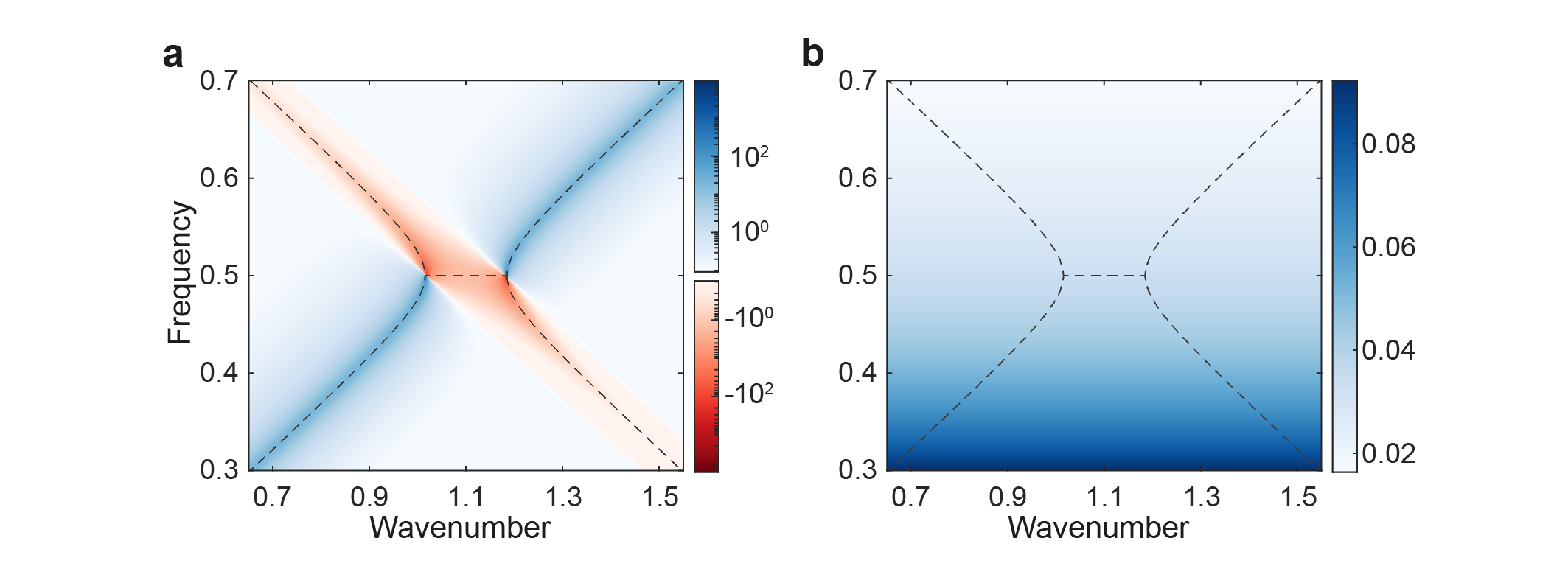
Figure B.1: $\mathrm{kDOS}$ maps for a PTC with sinusoidally-modulated relative permittivity, $\epsilon(t)=\epsilon_{0}+\epsilon_{m}\sin(\Omega t)$, where the parameters are set to $\epsilon_{0}=5$, $\epsilon_{m}=1.5$, $\mu=1$, $\Omega=1$, and $\sigma=0.1$, indicating a small loss scenario ($\sigma<\sigma_{c}$). Panel (a) displays the $\mathrm{kDOS}$ when the wavevector $\mathbf{k}$ is perpendicular to the dipole orientation vector $\mathbf{n}_{\mathbf{p}}$. Panel (b) examines the $\mathrm{kDOS}$ when $\mathbf{k}$ is parallel to $\mathbf{n}_{\mathbf{p}}$.

C   Pseudo-Hermiticity of PTCs

Under the source-free condition, Maxwell’s equations (Eqs. (1) and (2)) for a plane electromagnetic wave can be reformulated into the following matrix differential equation:

$$\begin{bmatrix}0&k\\ k&0\end{bmatrix}\begin{bmatrix}E\\ H\end{bmatrix}=-i\frac{\partial}{\partial t}\begin{bmatrix}\epsilon(t)&0\\ 0&\mu\end{bmatrix}\begin{bmatrix}E\\ H\end{bmatrix}-i\begin{bmatrix}\sigma&0\\ 0&0\end{bmatrix}\begin{bmatrix}E\\ H\end{bmatrix}.$$ (S19)

Due to the time-periodic variation in permittivity, the solutions to Eq. (S19) can be represented as a Floquet state: $\ket{\Psi(t)}=[E\;H]^{T}=e^{-i\omega t}\ket{\Phi(t)}$, where $\ket{\Phi(t)}=\ket{\Phi(t+T)}$. Substituting $\ket{\Psi(t)}$ into Eq. (S19) yields

$$\omega\ket{\Phi(t)}=\left[-i\frac{\partial}{\partial t}-\frac{k}{\mu\epsilon(t)}\begin{bmatrix}0&\mu\\ \epsilon(t)&0\end{bmatrix}-\frac{i\{\dot{\epsilon}(t)+\sigma\}}{2\epsilon(t)}(\mathbb{I}_{2}+\mathbf{\sigma}_{z})\right]\ket{\Phi(t)},$$ (S20)

where $\mathbb{I}_{2}$ denotes the identity matrix and $\sigma_{i}$ represents the Pauli matrix. Next we define a non-periodic state $\ket{\Phi_{N}(t)}$ as follows:

$$\ket{\Phi_{N}(t)} \equiv\exp(\int\frac{\dot{\epsilon}(t)+\sigma}{2\epsilon(t)}dt)\ket{\Phi(t)}$$ (S21)

$$=\exp(\frac{a_{0}\sigma}{2}t)\exp{\frac{1}{2}\ln{\epsilon(t)}+i\frac{\sigma}{2}\sum_{n\neq 0}\frac{a_{n}}{n\Omega}e^{-in\Omega}}\ket{\Phi(t)}$$

$$\equiv\exp(\frac{a_{0}\sigma}{2}t)\ket{\Phi_{P}(t)},$$

where the $a_{n}$’s are the Fourier expansion coefficients of $1/\epsilon(t)$, i.e., $1/\epsilon(t)=\sum_{n}a_{n}e^{-in\Omega t}$. Here, it can be shown that $\ket{\Phi_{P}(t)}$ is time-periodic with the periodicity of $T$, i.e., $\ket{\Phi_{P}(t)}=\ket{\Phi_{P}(t+T)}$. Then, Eqs. (S20) and (S21) can be reformulated into the following eigenvalue equation:

$$\left(\omega+\frac{ia_{0}\sigma}{2}\right)\ket{\Phi_{P}(t)} =\left[-i\frac{\partial}{\partial t}-\frac{k}{\mu\epsilon(t)}\begin{bmatrix}0&\mu\\ \epsilon(t)&0\end{bmatrix}-\frac{i\{\dot{\epsilon}(t)+\sigma\}}{2\epsilon(t)}\sigma_{z}\right]\ket{\Phi_{P}(t)}$$ (S22)

$$=\mathcal{H}_{\mathrm{e}}(t)\ket{\Phi_{P}(t)},$$

where the effective Hamiltonian matrix $\mathcal{H}_{\mathrm{e}}(t)$ can be shown to be $\sigma_{x}$-pseudo-Hermitian, i.e., $\mathcal{H}^{\dagger}_{\mathrm{e}}=\sigma_{x}\mathcal{H}_{\mathrm{e}}\sigma_{x}^{-1}$.

D   Analysis with driven Lorentz model

In this section, we utilize a driven Lorentz oscillator model to demonstrate that we can obtain results qualitatively similar to those presented in the main text. Within this model, the polarization density $\mathbf{P}$ and the electric field $\mathbf{E}$ are described by the following equation:

$$\frac{\partial^{2}\mathbf{P}}{\partial t^{2}}+\eta\frac{\partial\mathbf{P}}{\partial t}+\frac{\kappa(t)}{m}\mathbf{P}=\frac{Ne^{2}}{m}\mathbf{E},$$ (S23)

where $N$ represents the number of atoms per unit volume, $m$ denotes the mass of the bound charge, $\eta$ is the damping coefficient, and $e$ is the elementary charge. The elastic constant, $\kappa(t)$, is considered to be time-periodic with a period $T=2\pi/\Omega$. The PTC can be analyzed by solving Maxwell’s equations in conjunction with the driven Lorentz model:

$$\nabla\times\mathbf{H} =\frac{\partial\mathbf{D}}{\partial t}+\mathbf{J},\quad\mathbf{D}=\epsilon_{v}\mathbf{E}+\mathbf{P},$$ (S24)

$$\nabla\times\mathbf{E} =-\frac{\partial\mathbf{B}}{\partial t},\quad\mathbf{B}=\mu_{v}\mathbf{H}.$$

To simplify the analysis, we focus here on the one-dimensional case. Considering an extended current source $\mathbf{J}(\mathbf{r},t)=\mathrm{Re}[Je^{i(kx-\omega t)}]\hat{\mathbf{z}}$, we can assume the electric and magnetic fields, as well as the polarization density, as follows: $\mathbf{E}(\mathbf{r},t)=\mathrm{Re}[E(t)e^{ikx}]\hat{\mathbf{z}}$, $\mathbf{H}(\mathbf{r},t)=\mathrm{Re}[H(t)e^{ikx}]\hat{\mathbf{y}}$, and $\mathbf{P}(\mathbf{r},t)=\mathrm{Re}[P(t)e^{ikx}]\hat{\mathbf{z}}$. These assumptions simplify Eqs (S23) and (S24) into the following matrix differential equation:

$$i\frac{\partial}{\partial t}\ket{a(t)}=A(t)\ket{a(t)}+\ket{S(t)},$$ (S25)

where

$$A(t)=\begin{bmatrix}0&-\frac{k}{\epsilon_{v}}&0&-i\frac{1}{\epsilon_{v}}\\ -\frac{k}{\mu_{v}}&0&0&0\\ 0&0&0&i\\ i\frac{Ne^{2}}{m}&0&-i\frac{\kappa(t)}{m}&-i\eta\end{bmatrix},\ \ket{a(t)}=\begin{bmatrix}E(t)\\ H(t)\\ P(t)\\ \dot{P}(t)\end{bmatrix},$$ (S26)

and

$$\ket{S(t)}=-i\frac{J}{\epsilon_{v}}\begin{bmatrix}1\\ 0\\ 0\\ 0\end{bmatrix}e^{-i\omega t}.$$ (S27)

By defining the following matrix $R$ as,

$$R=\begin{bmatrix}\sqrt{\epsilon_{v}}&\sqrt{\mu_{v}}&0&0\\ \sqrt{\epsilon_{v}}&-\sqrt{\mu_{v}}&0&0\\ 0&0&\sqrt{\frac{\kappa_{0}}{Ne^{2}}}&i\sqrt{\frac{m}{Ne^{2}}}\\ 0&0&\sqrt{\frac{\kappa_{0}}{Ne^{2}}}&-i\sqrt{\frac{m}{Ne^{2}}}\\ \end{bmatrix},$$ (S28)

Maxwell’s equations can be transformed into a Schrödinger-like equation:

$$i\frac{\partial}{\partial t}\ket{\Psi(t)}=\mathcal{H}(t)\ket{\Psi(t)}+\ket{s(t)},$$ (S29)

where $\mathcal{H}(t)=RA(t)R^{-1}$, $\ket{\Psi(t)}=R\ket{a(t)}$, and $\ket{s(t)}=R\ket{S(t)}=\ket{s}e^{-i\omega t}$. When the elastic constant remains constant (i.e., $\kappa(t)=\kappa_{0}$ in Eq. (S23)), the band structure of the time-invariant medium can be determined using Eqs. (S23) and (S24). The resulting band structure, shown in the top panel of Fig. D.1, illustrates the presence of an energy gap resulting from the avoided crossing.

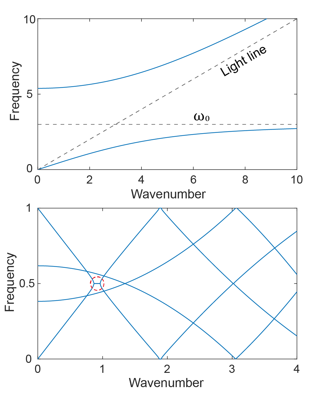
Figure D.1: The band structure derived from an undriven Lorentz model (upper panel) is shown alongside the Floquet band structure from a driven Lorentz model (lower panel). In the driven Lorentz model, the elastic constant is modeled as $\kappa(t)=\kappa_{0}+\kappa_{m}\sin(\Omega t)$. The band structures are plotted using the following fictitious parameters: $\kappa_{0}=9$, $\kappa_{m}=1.8$, $N=20$, $m=1$, $e=-1$, and $\Omega=1$. Additionally, the vacuum permittivity and permeability are assumed to be 1.

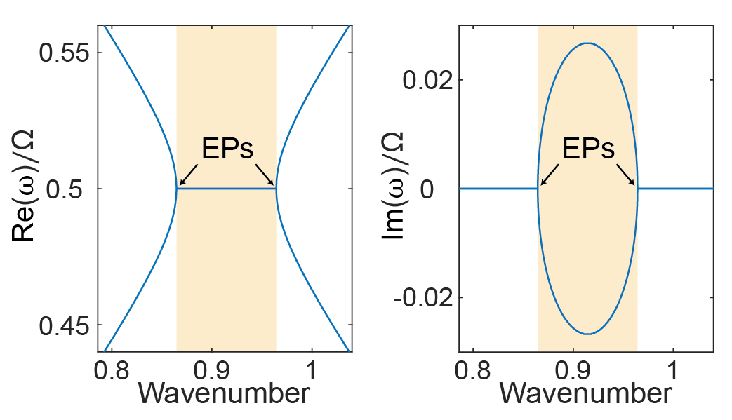
Figure D.2: Illustration of the Floquet band structure near the momentum gap of the PTC as described by the driven Lorentz model. The plots are generated under the assumption of a lossless case, where $\eta=0$.

When the elastic constant is modulated in a time-periodic manner, the field vector solutions to the Schrödinger-like equation take the form of a Floquet state, i.e., $\ket{\Psi(t)}=e^{-i\omega t}\ket{\Phi(t)}$. Here, $\ket{\Phi(t)}$ exhibits the same periodicity as the Hamiltonian matrix $\mathcal{H}(t)$, enabling the Fourier expansion of $\ket{\Phi(t)}$ as $\ket{\Phi(t)}=\sum_{n}{e^{-in\Omega t}\ket{\phi_{n}}}$. Additionally, the time-periodic Hamiltonian matrix can be expanded as $\mathcal{H}(t)=\sum_{m}{e^{-im\Omega t}\mathcal{H}_{m}}$. Substituting the expanded Hamiltonian matrix and field vectors into the Schrödinger-like equation reveals that:

$$(\omega+n\Omega)\ket{\phi_{n}}=\begin{cases}\sum_{m}{\mathcal{H}_{n-m}\ket{\phi_{m}}}+\ket{s},&\text{if }n=0\\ \sum_{m}{\mathcal{H}_{n-m}\ket{\phi_{m}}},&\text{otherwise}\end{cases}$$ (S30)

where $n$ and $m$ are integers. The above system of linear equations can be recast into the following matrix equation similar to that given in the previous section:

$$\omega\ket{F}=\mathcal{H}_{F}\ket{F}+\ket{s_{F}},$$ (S31)

where $\ket{s_{F}}$ is a column vector defined as $\ket{s_{F}}=[\cdots;0;\ket{s};0;\cdots]$, and the Floquet Hamiltonian matrix, $\mathcal{H}_{F}$, is expressed as

$$\mathcal{H}_{F}=\begin{bmatrix}\ddots&\ddots&&&\\ \ddots&\mathcal{H}_{0}+\Omega I&\mathcal{H}_{-1}&\mathcal{H}_{-2}&\\ &\mathcal{H}_{+1}&\mathcal{H}_{0}&\mathcal{H}_{-1}&\\ &\mathcal{H}_{+2}&\mathcal{H}_{+1}&\mathcal{H}_{0}-\Omega I&\ddots\\ &&&\ddots&\ddots\end{bmatrix}.$$ (S32)

The Floquet band structure, characterized by complex-valued quasi-eigenfrequencies, can be calculated by solving the following eigenvalue problem under a source-free condition ($J=0$):

$$\mathcal{H}_{F}\ket{R}=\omega\ket{R}.$$ (S33)

When employing a driven Lorentz model with a sinusoidally varying elastic constant, the matrices $\mathcal{H}_{\pm m}$, which describe the coupling between the original bands and the Floquet sidebands, are zero for all non-zero integer values of $m$, except for $m=1$. This indicates that only adjacent bands interact. As illustrated in the bottom panel of Figure D.1, the Floquet band structure reveals the emergence of a momentum gap, highlighted by the red dashed circle. This momentum gap emerges at the intersection of the original positive frequency band and the first-order Floquet sideband of the negative frequency band. Figure D.2 illustrates the Floquet band structure in the vicinity of this momentum gap.

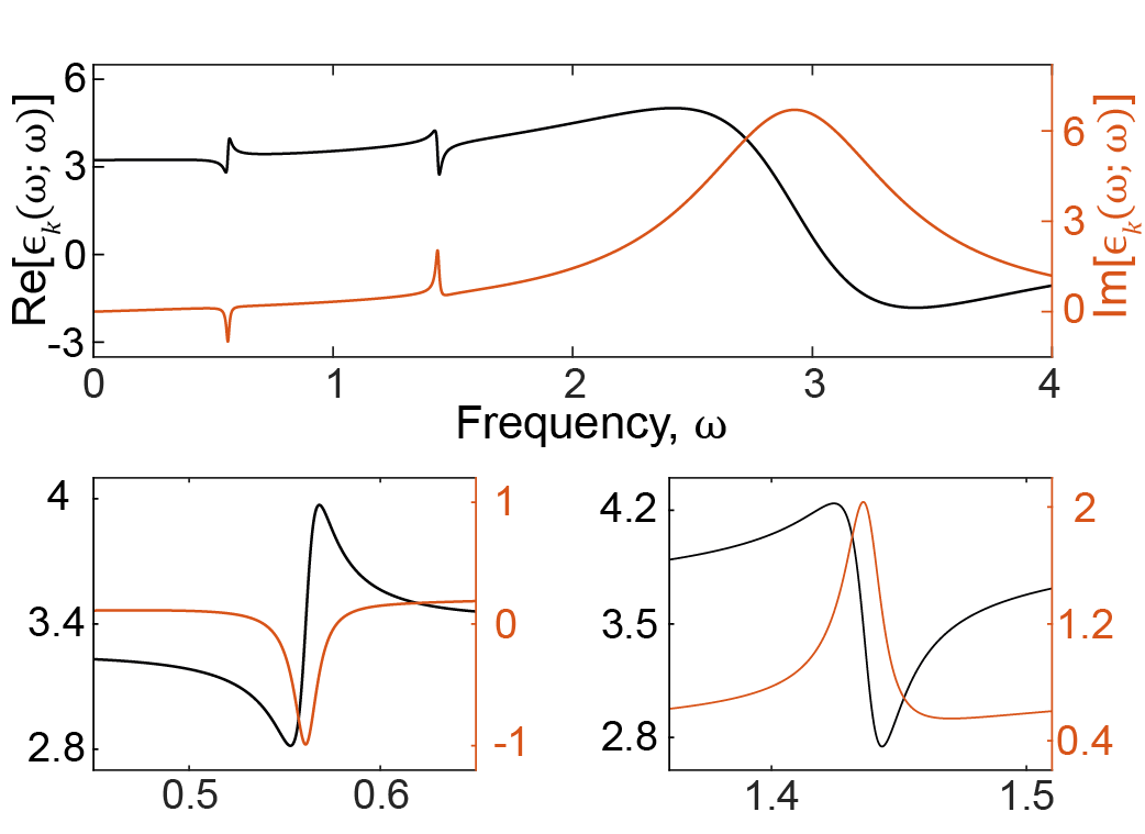
Figure D.3: The complex-valued relative permittivity in the case of small intrinsic loss: $\eta=0.9<\eta_{c}$. For this plot, the wavenumber is fixed at $k=0.8$.

Next, we investigate the low-loss case, characterized by $\eta=0.9$, which is less than the critical value $\eta_{c}$. By applying Eq. (S31), we calculate the complex-valued, momentum-resolved relative permittivity, defined as $\epsilon(k,\omega)=1+P_{0}/E_{0}$, and present it in Fig. D.3 for a fixed wavenumber $k=0.8$. Besides the fundamental Lorentzian resonance at $\omega_{0}=\sqrt{\kappa_{0}/m}$, two additional Lorentzian-like resonances emerge due to the time-periodic modulation, as specifically illustrated in Fig. D.3. The resonance at the lower frequency is attributed to the Floquet sideband of the negative frequency band, whereas the resonance at the higher frequency is related to the Floquet sideband of the positive frequency band. Notably, near the lower frequency resonance, the imaginary part of the relative permittivity becomes negative, indicating net gain. This region of net gain corresponds to the negative $\mathrm{kDOS}$ region identified through power flow analysis. Figure D.4 illustrates the maps of $\bar{P}_{l}(k,\omega)$ and $\bar{P}_{g}(k,\omega)$ for a case of small intrinsic loss. The SE decay and excitation rates, shown in the left panels, demonstrate significant qualitative agreement with the results derived from the nondispersive model discussed in the main text.

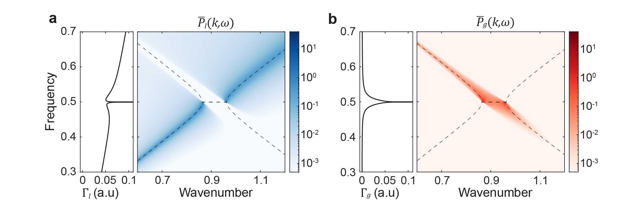
Figure D.4: Maps of $\bar{P}_{l}(k,\omega)$ and $\bar{P}_{g}(k,\omega)$, along with SE decay and excitation rates, for $\eta=0.9$ (indicating a case of small intrinsic loss).

E   $\mathrm{kDOS}$ decomposition within momentum gap

In this section, we focus on the decomposition of $\mathrm{kDOS}$ when the wavenumber is located within the central gap region ( $k_{EP_{-}}<\mathbf{k}<k_{EP_{+}}$). When considering only the two bands involved in the formation of the momentum gap, it is no longer valid to assume that $\mathrm{Im}[I_{\alpha}]$ is negligible for this range of wavenumbers. Consequently, the $\mathrm{kDOS}$ is expressed as follows:

$$\rho_{\mathbf{p}}(\mathbf{k},\omega)\approx\sum_{\alpha=\pm}\rho_{\mathbf{p},\mathrm{Re}}^{\alpha}(\mathbf{k},\omega)+\rho_{\mathbf{p},\mathrm{Im}}^{\alpha}(\mathbf{k},\omega),$$ (S34)

where two constituting $\rho_{\mathbf{p}}(\mathbf{k},\omega)$ terms are given by,

$$\rho_{\mathbf{p},\mathrm{Re}}^{\alpha}(\mathbf{k},\omega)=\frac{1}{\pi}\frac{\gamma_{\alpha}}{(\omega-\Omega_{\alpha})^{2}+\gamma_{\alpha}^{2}}\mathrm{Re}[I_{\alpha}(\mathbf{k})],$$ (S35)

$$\rho_{\mathbf{p},\mathrm{Im}}^{\alpha}(\mathbf{k},\omega)=\frac{1}{\pi}\frac{\Omega_{\alpha}-\omega}{(\omega-\Omega_{\alpha})^{2}+\gamma_{\alpha}^{2}}\mathrm{Im}[I_{\alpha}(\mathbf{k})].$$

Figure E.1 shows the $\mathrm{kDOS}$ and its decomposition for a case with low intrinsic loss, specifically when $\sigma=0.1$.

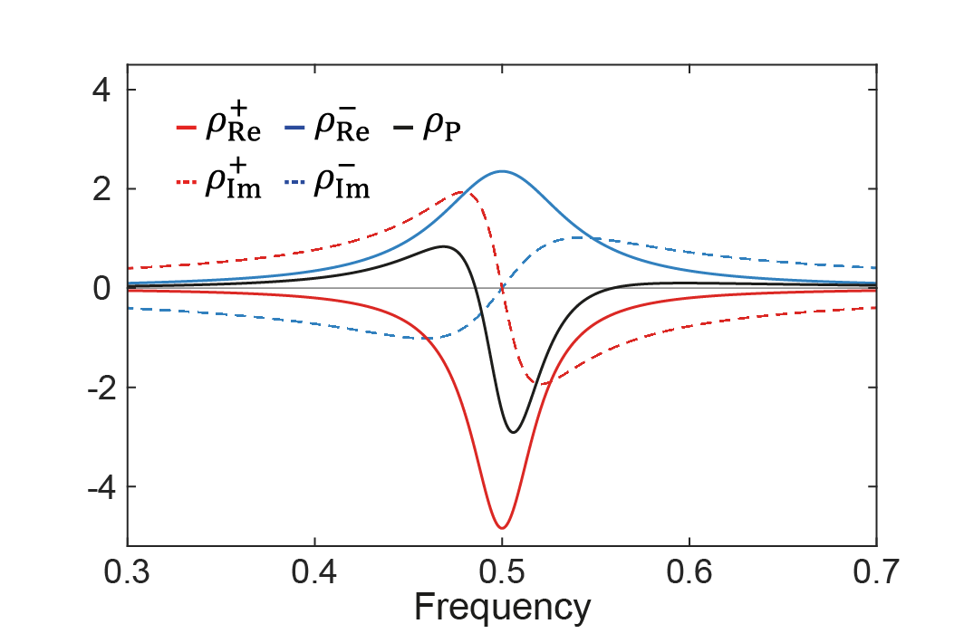
Figure E.1: $\mathrm{kDOS}$ and its decomposition plotted as a function of frequency at $k=1.05$ for the case of low intrinsic loss, i.e., $\sigma=0.1<\sigma_{c}$.

F   Non-orthogonality of Floquet eigenstates

Due to the non-Hermiticity of the Floquet Hamiltonian matrix, the Floquet eigenstates $\ket{\Phi_{m}^{\alpha}(t)}$ are generally no longer orthogonal. Here, the integer $m$ denotes Floquet index and $\alpha=\pm$ label the bands according to their propagation directions. Inside the momentum gap, the bands are indistinguishable by propagation direction. Therefore, we label the band with a smaller imaginary part of the eigenfrequency as $\alpha=+$. The extended inner product between two Floquet eigenstates are defined as,

$$\langle\langle\Phi_{m}^{\alpha}(t)|\Phi_{n}^{\beta}(t)\rangle\rangle=\frac{1}{T}\int_{0}^{T}{dt\innerproduct{\Phi_{m}^{\alpha}(t)}{\Phi_{n}^{\beta}(t)}}$$ (S36)

The integrand can be expressed as,

$$\innerproduct{\Phi_{m}^{\alpha}(t)}{\Phi_{n}^{\beta}(t)}$$

$$=\left(\sum_{p}{e^{i(p-m)\Omega t}\bra{\phi_{p}^{\alpha}}}\right)\left(\sum_{p}{e^{-i(p-n)\Omega t}\ket{\phi_{p}^{\beta}}}\right)$$

$$=\sum_{p}{\sum_{q}{e^{-i(p-2q-m+n)\Omega t}\innerproduct{\phi_{p-q}^{\alpha}}{\phi_{q}^{\beta}}}}$$ (S37)

After time-averaging, only the terms with $p-2q-m+n=0$ remain, yielding

$$\langle\langle\Phi_{m}^{\alpha}(t)|\Phi_{n}^{\beta}(t)\rangle\rangle =\sum_{q}{\innerproduct{\phi_{q+m-n}^{\alpha}}{\phi_{q}^{\beta}}}$$ (S38)

$$=\sum_{q}{\innerproduct{\phi_{q+m}^{\alpha}}{\phi_{q+n}^{\beta}}}$$ (S39)

The inner product of the Floquet (right) eigenvectors, on the other hand, can be expressed as,

$$\innerproduct{R_{m}^{\alpha}}{R_{n}^{\beta}}=\sum_{q}{\innerproduct{\phi_{q+m}^{\alpha}}{\phi_{q+n}^{\beta}}}$$ (S40)

As a result, the inner product of the Floquet right eigenvectors is equivalent to the suitably extended inner product of the Floquet eigenstates. Because the Floquet Hamiltonian matrix is non-Hermitian, the Floquet eigenstates of PTCs are generally non-orthogonal to each other when the wavenumber is fixed. The Petermann factor ($\mathrm{PF}$) is a measure of non-orthogonality in a non-Hermitian system that was originally introduced to quantify the excess noise induced by the non-orthogonal resonant modes of unstable cavities[41, 42, 43]. In our case, the $\mathrm{PF}$ can be written as,

$$\mathrm{PF}=\frac{\innerproduct{R_{m}^{\alpha}}{R_{m}^{\alpha}}\innerproduct{L_{m}^{\alpha}}{L_{m}^{\alpha}}}{\left|\innerproduct{L_{m}^{\alpha}}{R_{m}^{\alpha}}\right|^{2}}$$ (S41)

where the Floquet left eigenvectors $\bra{L_{m}^{\alpha}}$ are defined as the solutions of the following eigenvalue equation,

$$\bra{L_{m}^{\alpha}}\mathcal{H}_{F}=\bra{L_{m}^{\alpha}}\omega_{m}^{\alpha}$$ (S42)

Figure F.1 shows the $\mathrm{PF}$ for the band indicated by the red arrow in the inset calculated from Eq.(S41). The $\mathrm{PF}$ diverges as the wavenumber approaches the gap edges because of the vanishing overlap between Floquet left and right eigenvectors $\innerproduct{L_{m}^{\alpha}}{R_{m}^{\alpha}}$.

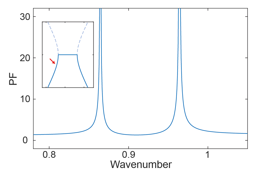
Figure F.1: PF calculated along the band indicated by the red arrow in the inset

G   $\mathrm{kDOS}$ at EPs

In this section, we follow the methodology outlined in [47] to derive the $\mathrm{kDOS}$ at the edge of the momentum gap. Precisely at $\mathbf{k_{EP_{+}}}$ (i.e., the right edge of the momentum gap), the Floquet Hamiltonian matrix assumes the form of a defective matrix, which we denote as $\mathcal{H}_{F}^{0}$. The right Floquet eigenvector and its corresponding right Jordan vector at the exceptional point (EP) can be described by

$$\mathcal{H}_{F}^{0}\ket{R^{0}} =\omega_{0}\ket{R^{0}}$$ (S43)

$$\mathcal{H}_{F}^{0}\ket{J_{R}^{0}} =\omega_{0}\ket{J_{R}^{0}}+\ket{R^{0}}.$$

Here, $\omega_{0}=\Omega_{0}-i\gamma_{0}$ denotes the degenerate quasi-eigenfrequency at the EP. In the vicinity of $\mathbf{k_{EP_{+}}}$ (specifically, $|\mathbf{k}|=k_{EP_{+}}+\lambda$, where $\lambda\ll 1$), the Floquet Hamiltonian matrix is expanded as $\mathcal{H}_{F}(\lambda)=\mathcal{H}_{F}^{0}+\lambda\mathcal{H}_{F}^{1}$. The eigenvalue equation for this near-EP regime is given by:

$$\mathcal{H}_{F}(\lambda)\ket{R^{\pm}}=\omega_{\pm}\ket{R^{\pm}}.$$ (S44)

Near the second-order EP, it is posited that both the quasi-eigenfrequencies and the right Floquet eigenvectors can be expressed using alternating Puiseux series, as described in [47]:

$$\omega_{\pm} =\omega_{0}\pm\lambda^{1/2}\omega_{1}+\lambda\omega_{2}\pm\lambda^{3/2}\omega_{3}+\cdots$$ (S45)

$$\ket{R^{\pm}} =\ket{R^{0}}\pm\lambda^{1/2}\ket{R^{1}}+\lambda\ket{R^{2}}\pm\cdots.$$

By inserting Eq. (S45) into Eq. (S44) and matching the coefficients of $\lambda^{1/2}$ and $\lambda$, we infer that

$$\omega_{\pm} =\omega_{0}\pm\lambda^{1/2}\Delta+\mathcal{O}(\lambda)$$ (S46)

$$\ket{R^{\pm}} =\ket{R^{0}}\pm\lambda^{1/2}\Delta\ket{J_{R}^{0}}+\mathcal{O}(\lambda),$$

where $\Delta=(\bra{L^{0}}\mathcal{H}_{F}^{1}\ket{R^{0}}/\innerproduct{J_{L}^{0}}{R^{0}})^{1/2}$. The same analysis can be applied to the left Floquet vector and the left Jordan vector. Utilizing Eq. (S46), the Green’s function at $\mathbf{k_{EP_{+}}}$ can be calculated as follows:

$$\mathcal{G}_{F}(\mathbf{k_{EP_{+}}},\omega) \approx\lim_{\lambda\rightarrow 0}\left[\sum_{\alpha=\pm}\frac{1}{\omega-\omega_{\alpha}}\frac{\ket{R^{\alpha}}\bra{L^{\alpha}}}{\innerproduct{L^{\alpha}}{R^{\alpha}}}\right]=$$ (S47)

$$\frac{2}{(\omega-\omega_{0})^{2}}\frac{\ket{R^{0}}\bra{L^{0}}}{\innerproduct{L^{0}}{J_{R}^{0}}+\innerproduct{J_{L}^{0}}{R^{0}}}+\frac{2}{\omega-\omega_{0}}\frac{\ket{R^{0}}\bra{J_{L}^{0}}+\ket{J_{R}^{0}}\bra{L^{0}}}{\innerproduct{L^{0}}{J_{R}^{0}}+\innerproduct{J_{L}^{0}}{R^{0}}}.$$

Then, $\rho_{\mathbf{p}}(\mathbf{k_{EP_{+}}},\omega)$ is expressed as follows:

$$\rho_{\mathbf{p}}(\mathbf{k_{EP_{+}}},\omega) \approx\frac{2\epsilon_{0}\mu\omega}{\pi}\mathrm{Im}[\mathbf{n}_{\mathbf{p}}\cdot\mathbb{G}_{0}(\mathbf{k_{EP_{+}}},\omega)\cdot\mathbf{n}_{\mathbf{p}}]$$ (S48)

$$\approx\frac{2}{\pi}\frac{\{\gamma_{0}^{2}-(\omega-\Omega_{0})^{2}\}}{\{(\omega-\Omega_{0})^{2}+\gamma_{0}^{2}\}^{2}}\mathrm{Im}\left[\mathbf{n}_{\mathbf{p}}\cdot\left\{2\delta_{0}\cdot\frac{\ket{R^{0}}\bra{L^{0}}}{\innerproduct{L^{0}}{J_{R}^{0}}+\innerproduct{J_{L}^{0}}{R^{0}}}\cdot\epsilon_{0}A_{F}\otimes\mathbb{I}\right\}\cdot\mathbf{n}_{\mathbf{p}}\right]$$

$$+\frac{4}{\pi}\frac{\gamma_{0}(\omega-\Omega_{0})}{\{(\omega-\Omega_{0})^{2}+\gamma_{0}^{2}\}^{2}}\mathrm{Re}\left[\mathbf{n}_{\mathbf{p}}\cdot\left\{2\delta_{0}\cdot\frac{\ket{R^{0}}\bra{L^{0}}}{\innerproduct{L^{0}}{J_{R}^{0}}+\innerproduct{J_{L}^{0}}{R^{0}}}\cdot\epsilon_{0}A_{F}\otimes\mathbb{I}\right\}\cdot\mathbf{n}_{\mathbf{p}}\right]$$

$$+\frac{2}{\pi}\frac{\Omega_{0}-\omega}{(\omega-\Omega_{0})^{2}+\gamma_{0}^{2}}\mathrm{Im}\left[\mathbf{n}_{\mathbf{p}}\cdot\left\{2\delta_{0}\cdot\frac{(\ket{R^{0}}\bra{J_{L}^{0}}+\ket{J_{R}^{0}}\bra{L^{0}})}{\innerproduct{L^{0}}{J_{R}^{0}}+\innerproduct{J_{L}^{0}}{R^{0}}}\cdot\epsilon_{0}A_{F}\otimes\mathbb{I}\right\}\cdot\mathbf{n}_{\mathbf{p}}\right]$$

$$+\frac{2}{\pi}\frac{\gamma_{0}}{(\omega-\Omega_{0})^{2}+\gamma_{0}^{2}}\mathrm{Re}\left[\mathbf{n}_{\mathbf{p}}\cdot\left\{2\delta_{0}\cdot\frac{(\ket{R^{0}}\bra{J_{L}^{0}}+\ket{J_{R}^{0}}\bra{L^{0}})}{\innerproduct{L^{0}}{J_{R}^{0}}+\innerproduct{J_{L}^{0}}{R^{0}}}\cdot\epsilon_{0}A_{F}\otimes\mathbb{I}\right\}\cdot\mathbf{n}_{\mathbf{p}}\right].$$

References

Yablonovitch [1987]E. Yablonovitch, Inhibited spontaneous emission in solid-state physics and electronics, Phys. Rev. Lett. 58, 2059 (1987).
Joannopoulos et al. [1997]J. Joannopoulos, P. R. Villeneuve, and S. Fan, Photonic crystals, Solid State Communications 102, 165 (1997), highlights in Condensed Matter Physics and Materials Science.
Fan et al. [1997]S. Fan, P. R. Villeneuve, J. D. Joannopoulos, and E. F. Schubert, High extraction efficiency of spontaneous emission from slabs of photonic crystals, Phys. Rev. Lett. 78, 3294 (1997).
Petrov et al. [1998]E. P. Petrov, V. N. Bogomolov, I. I. Kalosha, and S. V. Gaponenko, Spontaneous emission of organic molecules embedded in a photonic crystal, Phys. Rev. Lett. 81, 77 (1998).
Boroditsky et al. [1999]M. Boroditsky, R. Vrijen, R. Coccioli, R. Bhat, and E. Yablonovitch, Spontaneous emission extraction and purcell enhancement from thin-film 2-d photonic crystals, J. Lightwave Technol. 17, 2096 (1999).
Li et al. [2000]Z.-Y. Li, L.-L. Lin, and Z.-Q. Zhang, Spontaneous emission from photonic crystals: Full vectorial calculations, Phys. Rev. Lett. 84, 4341 (2000).
Lodahl et al. [2004]P. Lodahl, A. Floris van Driel, I. S. Nikolaev, A. Irman, K. Overgaag, D. Vanmaekelbergh, and W. L. Vos, Controlling the dynamics of spontaneous emission from quantum dots by photonic crystals, Nature 430, 654 (2004).
Englund et al. [2005]D. Englund, D. Fattal, E. Waks, G. Solomon, B. Zhang, T. Nakaoka, Y. Arakawa, Y. Yamamoto, and J. Vučković, Controlling the spontaneous emission rate of single quantum dots in a two-dimensional photonic crystal, Phys. Rev. Lett. 95, 013904 (2005).
Altug et al. [2006]H. Altug, D. Englund, and J. Vučković, Ultrafast photonic crystal nanocavity laser, Nature physics 2, 484 (2006).
Lecamp et al. [2007]G. Lecamp, P. Lalanne, and J. P. Hugonin, Very large spontaneous-emission factors in photonic-crystal waveguides, Phys. Rev. Lett. 99, 023902 (2007).
Noda et al. [2007]S. Noda, M. Fujita, and T. Asano, Spontaneous-emission control by photonic crystals and nanocavities, Nature Photonics 1, 449 (2007).
Rao and Hughes [2007]V. S. C. M. Rao and S. Hughes, Single quantum dot spontaneous emission in a finite-size photonic crystal waveguide: Proposal for an efficient “on chip” single photon gun, Phys. Rev. Lett. 99, 193901 (2007).
Novotny and Hecht [2012]L. Novotny and B. Hecht, Principles of nano-optics (Cambridge university press, 2012).
Sauvan et al. [2013]C. Sauvan, J. P. Hugonin, I. S. Maksymov, and P. Lalanne, Theory of the spontaneous optical emission of nanosize photonic and plasmon resonators, Phys. Rev. Lett. 110, 237401 (2013).
Lin et al. [2016]Z. Lin, A. Pick, M. Lončar, and A. W. Rodriguez, Enhanced spontaneous emission at third-order dirac exceptional points in inverse-designed photonic crystals, Phys. Rev. Lett. 117, 107402 (2016).
Barnes et al. [2020]W. L. Barnes, S. A. Horsley, and W. L. Vos, Classical antennas, quantum emitters, and densities of optical states, Journal of Optics 22, 073501 (2020).
Purcell [1946]E. M. Purcell, Spontaneous emission probabilities at radio frequencies, Phys. Rev. 69, 674 (1946).
Martínez-Romero et al. [2016]J. S. Martínez-Romero, O. M. Becerra-Fuentes, and P. Halevi, Temporal photonic crystals with modulations of both permittivity and permeability, Phys. Rev. A 93, 063813 (2016).
Sounas and Alù [2017]D. L. Sounas and A. Alù, Non-reciprocal photonics based on time modulation, Nature Photonics 11, 774 (2017).
Wang et al. [2018]N. Wang, Z.-Q. Zhang, and C. T. Chan, Photonic floquet media with a complex time-periodic permittivity, Phys. Rev. B 98, 085142 (2018).
Chamanara et al. [2018]N. Chamanara, Z. L. Deck-Léger, C. Caloz, and D. Kalluri, Unusual electromagnetic modes in space-time-modulated dispersion-engineered media, Physical Review A 97, 10.1103/PhysRevA.97.063829 (2018), arXiv:1710.01625 .
Shcherbakov et al. [2019]M. R. Shcherbakov, K. Werner, Z. Fan, N. Talisa, E. Chowdhury, and G. Shvets, Photon acceleration and tunable broadband harmonics generation in nonlinear time-dependent metasurfaces, Nature Communications 10, 1345 (2019).
Galiffi et al. [2019]E. Galiffi, P. A. Huidobro, and J. B. Pendry, Broadband nonreciprocal amplification in luminal metamaterials, Phys. Rev. Lett. 123, 206101 (2019).
Park and Min [2021]J. Park and B. Min, Spatiotemporal plane wave expansion method for arbitrary space–time periodic photonic media, Optics Letters 46, 484 (2021).
Lee et al. [2021]S. Lee, J. Park, H. Cho, Y. Wang, B. Kim, C. Daraio, and B. Min, Parametric oscillation of electromagnetic waves in momentum band gaps of a spatiotemporal crystal, Photonics Research 9, 142 (2021).
Lyubarov et al. [2022]M. Lyubarov, Y. Lumer, A. Dikopoltsev, E. Lustig, Y. Sharabi, and M. Segev, Amplified emission and lasing in photonic time crystals, Science 377, 425 (2022).
Park et al. [2022]J. Park, H. Cho, S. Lee, K. Lee, K. Lee, H. C. Park, J.-W. Ryu, N. Park, S. Jeon, and B. Min, Revealing non-hermitian band structure of photonic floquet media, Science Advances 8, eabo6220 (2022).
Wang et al. [2023]X. Wang, M. S. Mirmoosa, V. S. Asadchy, C. Rockstuhl, S. Fan, and S. A. Tretyakov, Metasurface-based realization of photonic time crystals, Science Advances 9, eadg7541 (2023).
Pendry et al. [2021]J. B. Pendry, E. Galiffi, and P. A. Huidobro, Gain in time-dependent media—a new mechanism, J. Opt. Soc. Am. B 38, 3360 (2021).
Galiffi et al. [2022]E. Galiffi, R. Tirole, S. Yin, H. Li, S. Vezzoli, P. A. Huidobro, M. G. Silveirinha, R. Sapienza, A. Alù, and J. Pendry, Photonics of time-varying media, Advanced Photonics 4, 014002 (2022).
Franke et al. [2021]S. Franke, J. Ren, M. Richter, A. Knorr, and S. Hughes, Fermi’s golden rule for spontaneous emission in absorptive and amplifying media, Phys. Rev. Lett. 127, 013602 (2021).
Ren et al. [2024]J. Ren, S. Franke, B. VanDrunen, and S. Hughes, Classical purcell factors and spontaneous emission decay rates in a linear gain medium, Phys. Rev. A 109, 013513 (2024).
Ren et al. [2021]J. Ren, S. Franke, and S. Hughes, Quasinormal modes, local density of states, and classical purcell factors for coupled loss-gain resonators, Physical Review X 11, 041020 (2021).
Vyshnevyy [2022]A. A. Vyshnevyy, Gain-dependent purcell enhancement, breakdown of einstein’s relations, and superradiance in nanolasers, Physical Review B 105, 085116 (2022).
Scarlatella et al. [2019]O. Scarlatella, A. A. Clerk, and M. Schiro, Spectral functions and negative density of states of a driven-dissipative nonlinear quantum resonator, New Journal of Physics 21, 043040 (2019).
Zhang et al. [2018]J. Zhang, B. Peng, Ş. K. Özdemir, K. Pichler, D. O. Krimer, G. Zhao, F. Nori, Y.-x. Liu, S. Rotter, and L. Yang, A phonon laser operating at an exceptional point, Nature Photonics 12, 479 (2018).
Wang et al. [2020]H. Wang, Y.-H. Lai, Z. Yuan, M.-G. Suh, and K. Vahala, Petermann-factor sensitivity limit near an exceptional point in a brillouin ring laser gyroscope, Nature communications 11, 1610 (2020).
Vuckovic et al. [1999]J. Vuckovic, O. Painter, Y. Xu, A. Yariv, and A. Scherer, Finite-difference time-domain calculation of the spontaneous emission coupling factor in optical microcavities, IEEE Journal of Quantum Electronics 35, 1168 (1999).
Pick et al. [2017]A. Pick, B. Zhen, O. D. Miller, C. W. Hsu, F. Hernandez, A. W. Rodriguez, M. Soljačić, and S. G. Johnson, General theory of spontaneous emission near exceptional points, Optics Express 25, 12325 (2017), arXiv:1604.06478 .
Ferrier et al. [2022]L. Ferrier, P. Bouteyre, A. Pick, S. Cueff, N. H. M. Dang, C. Diederichs, A. Belarouci, T. Benyattou, J. X. Zhao, R. Su, J. Xing, Q. Xiong, and H. S. Nguyen, Unveiling the Enhancement of Spontaneous Emission at Exceptional Points, Phys. Rev. Lett. 129, 83602 (2022).