On the rectilinear crossing number of complete balanced multipartite graphs and layered graphs

Abstract

A rectilinear drawing of a graph is a drawing of the graph in the plane in which the edges are drawn as straight-line segments. The rectilinear crossing number of a graph is the minimum number of pairs of edges that cross over all rectilinear drawings of the graph. Let $n\geq r$ be positive integers. The graph $K_{n}^{r}$, is the complete $r$-partite graph on $n$ vertices, in which every set of the partition has at least $\lfloor n/r\rfloor$ vertices. The layered graph, $L_{n}^{r}$, is an $r$-partite graph on $n$ vertices, in which for every $1\leq i\leq r-1$, all the vertices in the $i$-th partition are adjacent to all the vertices in the $(i+1)$-th partition. In this paper, we give upper bounds on the rectilinear crossing numbers of $K_{n}^{r}$ and $L_{n}^{r}$.

1 Introduction

Let $G$ be a graph on $n$ vertices and let $D$ be a drawing of $G$. The crossing number of $D$ is the number, $\operatorname{cr}(D)$, of pairs of edges that cross in $D$. The crossing number of $G$ is the minimum crossing number, $\operatorname{cr}(G)$, over all drawings of $G$ in the plane. A rectilinear drawing of $G$ is a drawing of $G$ in the plane in which its vertices are points in general position, and its edges are drawn as straight-line segments joining these points. The rectilinear crossing number of $G$, is the minimum crossing number, $\overline{\operatorname{cr}}(G)$, over all rectilinear drawings of $G$ in the plane. Computing crossing and rectilinear crossing numbers of graphs are important problems in Graph Theory and Combinatorial Geometry. For a comprehensive review of the literature on crossing numbers, we refer the reader to Schaefer’s book [2].

Most of the research on crossing numbers have been focused around the complete graph, $K_{n}$, and the complete bipartite graph $K_{n,m}$. For the complete graph, Hill [3] gave the following drawing of $K_{n}$; see Figure 1 for an example. Place half of the vertices equidistantly on the top circle of a cylinder, and the other half equidistantly on the bottom circle. Join the vertices with geodesics on the cylinder. Hill showed that the following number, $H(n)$, is the crossing number of this drawing, and it is now conjectured to be optimal. Let

$$H(n):=\frac{1}{4}\left\lfloor\frac{n}{2}\right\rfloor\left\lfloor\frac{n-1}{2}\right\rfloor\left\lfloor\frac{n-2}{2}\right\rfloor\left\lfloor\frac{n-3}{2}\right\rfloor.$$

Conjecture 1 (Harary-Hill [4])

$$\operatorname{cr}(K_{n})=H(n).$$

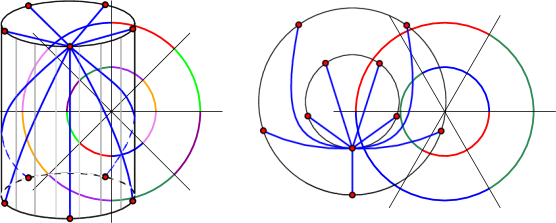
Figure 1: An example of Hill’s drawings of $K_{8}$, where here for convenience only the edges of one vertex are drawn. Left: The drawing on a cylinder. Right: An equivalent representation of Hill’s drawings via concentric cycles.

For the complete bipartite graph, Zarankiewicz gave a rectilinear drawing with the following number, $Z(n,m)$, as crossing number of this drawing, and it is now conjectured to be optimal. Let

$$Z(n,m):=\left\lfloor\frac{n}{2}\right\rfloor\left\lfloor\frac{n-1}{2}\right\rfloor\left\lfloor\frac{m}{2}\right\rfloor\left\lfloor\frac{m-1}{2}\right\rfloor$$

and

$$Z(n):=Z(n,n).$$

Conjecture 2 (Zarankiewicz [5])

$$\operatorname{cr}(K_{n,m})=Z(n,m).$$

The number $Z(n,m)$ is also conjectured to be the general optimal crossing number, directly implying the following conjecture.

Conjecture 3

$$\overline{\operatorname{cr}}(K_{n,m})=\operatorname{cr}(K_{n,m}).$$

Much less is known for the rectilinear crossing number of the complete graph. For $n\geq 10$, it is known that

$$\operatorname{cr}(K_{n})<\overline{\operatorname{cr}}(K_{n}).$$

In contrast to the case of the complete bipartite graph, there is no conjectured value for $\overline{\operatorname{cr}}(K_{n})$, nor drawings conjectured to be optimal. The best bounds to date are

$$0.379972\binom{n}{4}<\overline{\operatorname{cr}}(K_{n})<0.380445\binom{n}{4}+O(n^{3}).$$

The lower bound is due to Ábrego, Fernández-Merchant, Leaños, and Salazar [6], and the upper bound to Aichholzer, Duque, Fabila-Monroy, García-Quintero, and Hidalgo-Toscano [7]. It is known that

$$\lim_{n\to\infty}\frac{\overline{\operatorname{cr}}(K_{n})}{\binom{n}{4}}=\overline{q},$$

for some positive constant $\overline{q}$; this constant is known as the rectilinear crossing constant.

Let $K_{n_{1},n_{2},\dots,n_{r}}$ be the complete $r$-partite graph with $n_{i}$ vertices in the $i$-th set of the partition; and let $K_{n}^{r}$ be the complete balanced $r$-partite graph in which there are at least $\lfloor n/r\rfloor$ vertices in every partition set. Harborth [8] gave a drawing that provides an upper bound for $\operatorname{cr}(K_{n_{1},n_{2},\dots,n_{r}})$; and gave an explicit formula for this number. He claims that for the case of $r=3$, his drawing can be made rectilinear. More recently, Gethner, Hogben, Lidický, Pfender, Ruiz and Young [9] independently studied the problem of the crossing number and rectilinear crossing number of complete balanced $r$-partite graphs. For $r=3$, they obtain the same bound as Harborth; and their drawing is rectilinear.

Let $r$ be a positive integer and let $n$ be a multiple of $r$. The layered graph, $L_{n}^{r}$, is the graph defined as follows. Its vertex set is partitioned into sets $V_{1},\dots,V_{r}$, each consisting of $n/r$ vertices. We call the set $V_{i}$, the $i$-th layer of $L_{n}^{r}$. The edge set of $L_{n}^{r}$ is given by

$$\{uv:u\in L_{i}\textrm{ and }v\in L_{i+1},\textrm{ for }i=1,\dots,r-1\};$$

that is, the edges are exactly all possible edges between vertices on consecutive layers.

In this paper, we mainly focus on the rectilinear crossing numbers of $K_{n}^{r}$ and $L_{n}^{r}$ . If $n$ is fixed and $r$ tends to $n$, then $K_{n}^{r}$ tends to $K_{n}$. We believe that studying the rectilinear crossing number of $K_{n}^{r}$ might shed some light on how optimal rectilinear drawings of $K_{n}$ look like.

This paper is organized as follows. In Section 2, we give a general technique to obtain non-rectilinear and rectilinear drawings of a given graph $G$ on $n$ vertices. It simply consists of mapping randomly the vertices of $G$ to optimal drawings of $K_{n}$. We show how this technique upper bounds $\operatorname{cr}(K_{n}^{r})$ and $\overline{\operatorname{cr}}(K_{n}^{r})$. The bounds obtained in this way are very close to being optimal. However, for the layered graphs this technique gives rather poor upper bounds. In Section 3, we give a technique were given an specific drawing of a graph, we use this drawing as a “seed” to produce larger drawings by replacing each vertex $u$ with a cluster of collinear vertices $S_{u}$ arbitrarily close to $u$. In the new drawing two vertices in different clusters $S_{u}$ and $S_{v}$ are adjacent whenever $u$ and $v$ are adjacent in the original drawing. We call the new larger drawing a “planted drawing”. The conjectured crossing optimal drawings of $K_{n,n}$ and $K_{n,n,n}$ mentioned above are actually planted drawings with drawings of $K_{2,2}$ and $K_{2,2,2}$ as seeds, respectively. However, we show that there is no rectilinear drawing of $K_{4}$ or $K_{8}^{4}$ that can be the seed of a crossing optimal planted drawing of $K_{n}^{4}$. For the layered graph, we give a rectilinear planar drawing of $L_{2r}^{r}$. When used as a seed this drawing produces a planted drawing of $L_{n}^{r}$, with significantly smaller crossing number, than those produced by the random embedding technique. The proofs of many of our results are long and technical; for the sake of clarity, we have relocated most of the proofs and constructions to an appendix.

2 Random Embeddings into Drawings of $K_{n}$ with Small Crossing Number

Suppose that we have a drawing (that can be rectilinear but doesn’t have to be) $D^{\prime}$ of $K_{n}$. If $\operatorname{cr}(D^{\prime})$ is small, it might be a good idea to use this drawing to produce a drawing of a graph $G$ on $n$ vertices. Let $D$ be the drawing of $G$ that is produced by mapping the vertices of $G$ randomly to the vertices of $D^{\prime}$, and where the edges are drawn as their corresponding edges of $D^{\prime}$. We call $D$ a random embedding of $G$ into $D^{\prime}$.

In every $4$-tuple of vertices of $D^{\prime}$, there are three pairs of independent edges, which could cross. Of these three pairs at most one pair is crossing. For every pair of independent edges of $G$, we have a possible crossing in $D$; thus, the probability that this pair of edges is mapped to a pair of crossing edges is equal to

$$\frac{1}{3}\cdot\frac{\operatorname{cr}(D^{\prime})}{\binom{n}{4}}.$$

By defining, for every pair of independent edges of $G$, an indicator random variable with value equal to one if the edges cross and zero otherwise, we obtain the following result where $||G||$ is the number of edges in $G$ and $d(v)$ is the degree of a vertex $v$ of $G$.

Lemma 4

$$\operatorname{E}(\operatorname{cr}(D))=\frac{cr(D^{\prime})}{3\binom{n}{4}}\left(\binom{||G||}{2}-\sum_{v\in V(G)}\binom{d(v)}{2}\right).$$

Complete $r$-partite Graphs

For an upper bound on the crossing number of $K_{n}^{r}$, we use Lemma 4 and Hill’s drawing of $K_{n}$.

Theorem 5

Suppose that $n$ is a multiple of $r$. Let $D$ be a random embedding of $K_{n}^{r}$ into Hill’s drawing of $K_{n}$. Then,

$$\operatorname{cr}(K_{n}^{r})\leq E(\operatorname{cr}(D))\leq\frac{1}{16}\left(\frac{r-1}{r}\right)^{2}\left(\frac{n^{4}}{4}-\frac{3n^{3}}{2}\right)+O(n^{2}).$$

In [9], the authors obtain the same bound on $\operatorname{cr}(K_{n}^{r})$ by considering a random mapping of the vertices of $K_{n}^{r}$ into a sphere, and then joining the corresponding vertices with geodesics. This type of drawing is called a random geodesic spherical drawing. In 1965, Moon [10], showed that the expected number of crossings of a random geodesic spherical drawing of $K_{n}$ is equal to

$$\frac{1}{16}\binom{n}{2}\binom{n-2}{2}=H(n)-O(n^{3});$$

which explains why the bound of Theorem 5 matches the bound of [9].

Let $H(n,r)$ be the number of crossings in Harborth’s drawing for $\operatorname{cr}(K_{n}^{r})$. Due to the complexity of the formula, we use the following approximation to $H(n,r)$ instead.

Lemma 6

If $n$ is a multiple of $r$, then

$$H(n,r)\leq\frac{1}{16}\left(\frac{r-1}{r}\right)^{2}\left(\frac{n^{4}}{4}-2n^{3}\right)+O(n^{2}).$$

Let $D$ be as in Theorem 5; note that by Lemma 6, it holds that

$$E(\operatorname{cr}(D))-H(n,r)\leq\frac{1}{32}\left(\frac{r-1}{r}\right)^{2}n^{3}+O(n^{2})=O(n^{3}).$$

Thus, the random embedding gives an upper bound on $\operatorname{cr}(D)$ that matches the conjectured value up to the leading term, but it is a little worse in the lower terms.

We now upper bound $\overline{\operatorname{cr}}(K_{n}^{r})$, with this technique.

Theorem 7

Let $r$ be a positive integer and $n$ a multiple of $r$. Let $\overline{D}$ be a random embedding of $K_{n}^{r}$ into an optimal rectilinear drawing of $K_{n}$. Then

$$\overline{\operatorname{cr}}(K_{n}^{r}) \leq E(\operatorname{cr}(\overline{D}))$$

$$\leq\frac{\overline{q}}{4!}\left(\frac{r-1}{r}\right)^{2}n^{4}+o(n^{4})$$

$$<0.015852\left(\frac{r-1}{r}\right)^{2}n^{4}+o(n^{4}).$$

For a lower bound we have the following.

Theorem 8

Let $r$ be a positive integer and $n$ a multiple of $r$. Then

$$\overline{\operatorname{cr}}(K_{n}^{r})\geq\overline{\operatorname{cr}}(K_{r})\left(\frac{n}{r}\right)^{4}.$$

Theorems 7 and 8 imply the following.

Corollary 9

Let $r=r(n)$ be a monotone function of $n$ such that $r\to\infty$ as $n\to\infty$. Then

$$\lim_{n\to\infty}\frac{\overline{\operatorname{cr}}(K_{n}^{r})}{\binom{n}{4}}=\overline{q}.$$

In both [8] and [9], it is conjectured that

$$\operatorname{cr}\left(K_{n}^{3}\right)=\overline{\operatorname{cr}}\left(K_{n}^{3}\right).$$

Using the order type database [11], we have verified that

$$\overline{\operatorname{cr}}\left(K_{8}^{4}\right)=8\textrm{ and }\overline{\operatorname{cr}}\left(K_{9}^{4}\right)=15.$$

On the other hand

$$\operatorname{cr}\left(K_{8}^{4}\right)\leq H(8,4)=6\textrm{ and }\operatorname{cr}\left(K_{9}^{4}\right)\leq H(9,4)=15.$$

See Figure 2 for an example.

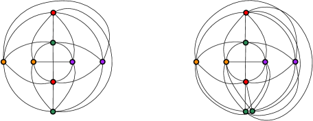
Figure 2: A drawing of $K_{8}^{4}$ with 6 crossings (left) and $K_{9}^{4}$ with 15 crossings (right).

From the above results we conjecture the following.

Conjecture 10

There exists a natural number $n_{0}>9$ such that for all $n\geq n_{0}$,

$$\operatorname{cr}\left(K_{n}^{4}\right)<\overline{\operatorname{cr}}\left(K_{n}^{4}\right).$$

Layered Graphs

Using the random embedding technique into Hill’s drawing of $K_{n}$, we obtain the following upper bound for $\operatorname{cr}(L_{n}^{r})$.

Theorem 11

$$\operatorname{cr}(L_{n}^{r})\leq\frac{(r-1)^{2}}{16r^{4}}n^{4}+O(n^{3}).$$

We improve this upper bound in Section 3.

3 Planted Rectilinear Drawings

Let $D$ be a rectilinear drawing of a graph $G$. For every vertex $v$ of $G$, let $\ell_{v}$, be a directed straight line passing through $v$ and no other vertex of $D$, such that to left of $\ell_{v}$ there are $\lfloor d(v)/2\rfloor$ neighbors of $v$ and to the right of $\ell_{v}$ there are the remaining $\lceil d(v)/2\rceil$ neighbors of $v$. Let $G^{s}$ be the graph whose vertex set is equal to

$$\{(v,i):i=1,\dots,s\textrm{ and }v\in V(G)\},$$

and in which $(v,i)$ is adjacent to $(w,j)$ whenever $vw$ is an edge of $G$. We say that the set $\{(v,1),\dots,(v,s)\}$ is the cluster of $v$. Let $D^{s}$ be the rectilinear drawing of $G^{s}$ in which for every vertex $v$ of $G$, the vertices its cluster are placed arbitrarily close to $\ell_{v}$ and arbitrarily close to $v$ (in $D$). We say that $D^{s}$ is a planted drawing of $G^{s}$ with seed $D$.

Lemma 12

$$\operatorname{cr}(D^{s})=\operatorname{cr}(D)s^{4}+\sum_{v\in V(G)}\left(\binom{\lfloor d(v)/2\rfloor}{2}+\binom{\lceil d(v)/2\rceil}{2}\right)\frac{s^{3}(s-1)}{2}+||G||\frac{s^{2}(s-1)^{2}}{4}.$$

Seeds and planted drawings were first used by Ábrego and Fernández-Merchant [12] to upper bound the rectilinear crossing number of $K_{n}$. The current best upper bound on $\overline{\operatorname{cr}}(K_{n})$ is obtained via a seed of 2643 vertices and 771218714414 crossings.

Complete $r$-partite Graphs

Note that if we use $K_{tr}^{r}$ as a seed for a planted drawing of $K_{n}^{r}$, we have that $s=\frac{n}{tr}$. Thus, from Lemma 12 we obtain the following.

Corollary 13

Let $D$ be a rectilinear drawing of $K_{tr}^{r}$. Then using $D$ as a seed we obtain a planted drawing of $K_{n}^{r}$ with

$$\left(\frac{\operatorname{cr}(D)+\frac{rt}{2}\left(\binom{\lfloor(r-1)t/2\rfloor}{2}+\binom{\lceil(r-1)t/2\rceil}{2}\right)+\frac{r(r-1)t^{2}}{8}}{(rt)^{4}}\right)n^{4}-O(n^{3})$$

crossings.

Using the seeds in Figure 3, we obtain planted rectilinear drawings of $K_{n}^{2}$ and $K_{n}^{3}$, with the conjectured minimum number of crossings.

Figure 3: The seeds for the planted drawings of $K_{n}^{2}$ and $K_{n}^{3}$

Using the random embedding technique and Theorem 5 we obtain a rectilinear drawing of $K_{n}^{4}$ with at most

$$0.0089676n^{4}+o(n^{4})$$ (1)

crossings; and since $\overline{q}>0.379972$, the best we can hope to achieve with the random embedding technique is a rectilinear drawing of $K_{n}^{4}$ with

$$0.0089055n^{4}+o(n^{4})$$ (2)

crossings.

Using a planar drawing of $K_{4}$ as a seed, we obtain a rectilinear planted drawing of $K_{n}^{r}$ with

$$\left(\frac{2\left(\binom{1}{2}+\binom{2}{2}\right)+\frac{3}{2}}{4^{4}}\right)n^{4}-O(n^{3})=\frac{7}{2^{9}}n^{4}-O(n^{3})=0.013671875n^{4}-O(n^{3})$$

crossings. Using a rectilinear drawing of $K_{8}^{4}$ with $8$ crossings, we obtain a planted rectilinear drawing with

$$\left(\frac{8+4\left(\binom{3}{2}+\binom{3}{2}\right)+6}{8^{4}}\right)n^{4}-O(n^{3})=\frac{38}{8^{4}}n^{4}-O(n^{3})=0.009277344n^{4}-O(n^{3})$$

crossings.

Fabila-Monroy and López [13] used an heuristic of randomly moving vertices to obtain a rectilinear drawing of $K_{75}$ with $45049$ crossings. This was used as a seed for a previous best upper bound on $\overline{q}$. In [14] Duque, Fabila-Monroy, Hernández-Vélez and Hidalgo-Toscano gave an $O(n^{2}\log n)$ time algorithm to compute the crossing number of a rectilinear drawing of a graph on $n$ vertices. Using a similar heuristic as in [13] and the algorithm of [14], we obtained a rectilinear drawing of $K_{24}^{4}$ with $2033$ crossings. Using this as a seed we obtain a planted rectilinear drawing of $K_{n}^{4}$ with

$$\left(\frac{2033+12\left(\binom{9}{2}+\binom{9}{2}\right)+54}{24^{4}}\right)n^{4}-O(n^{3})=\frac{2951}{24^{4}}n^{4}-O(n^{3})=0.0088946n^{4}-O(n^{3})$$

crossings. This is better than the best possible upper bound obtainable with the random embedding technique. However, for $r\geq 5$, we have not found seeds that provide planted drawings with less crossings than the drawings obtained from the random embedding technique.

Layered Graphs

We now show a rectilinear planar drawing $D_{r}$ of $L_{2r}^{r}$. For $i=1,\dots,r$, let $\{u_{i},v_{i}\}$ be the two vertices on layer $i$ of $L_{2r}^{r}$. Place $u_{i}$ and $v_{i}$ at the points $p_{i}$ and $q_{i}$, respectively; where

$$p_{i}:=\begin{cases}(i,0)\textrm{ if }i\textrm{ is odd, }\\ (0,i)\textrm{ if }i\textrm{ is even,}\end{cases}\textrm{ and }\ q_{i}:=\begin{cases}(-i,0)\textrm{ if }i\textrm{ is odd, }\\ (0,-i)\textrm{ if }i\textrm{ is even.}\end{cases}$$

See Figure 4 for the drawing of $L_{12}^{6}$.

Figure 4: The rectilinear $D_{6}$ drawing of $L_{12}^{6}$

Using this drawing as a seed for a planted drawing of $L_{n}^{r}$, we obtain a rectilinear drawing with

$$\sum_{v\in V(D_{r})}\left(\binom{\lfloor d(v)/2\rfloor}{2}+\binom{\lceil d(v)/2\rceil}{2}\right)\frac{s^{4}}{2}+||D_{r}||\frac{s^{4}}{4}-O(s^{3})$$

$$=(2(r-2)\cdot 2)\frac{n^{4}}{2\cdot(2r)^{4}}+4\cdot(r-1)\frac{n^{4}}{4\cdot(2r)^{4}}-O(n^{3})$$

$$=\frac{3r-5}{16r^{4}}n^{4}-O(n^{3})$$

crossings. For $r\geq 4$, this is better than the upper bound obtained with the random embedding technique.

For $i=2,\dots,r-1$, let $H_{i}$ be the subgraph of $L_{n}^{r}$ induced by the vertices in layers $i-1,i$ and $i+1$. Note that this graph isomorphic to $K_{n/r,2n/r}$. Thus, assuming that Zarankiewicz’s conjecture holds, in every drawing of $L_{n}^{r}$, $H_{i}$ produces at least $Z(n/r,2n/r)$ crossings. Each of these crossings is produced by at most two such $H_{i}$’s. Therefore, assuming that Zarankiewicz’s conjecture is true, we have that

$$\operatorname{cr}(L_{n}^{r})\geq\frac{(r-2)}{2}Z(n/r,2n/r)=\frac{2r-4}{16r^{4}}n^{4}-O(n^{3}).$$

4 Appendix

We continuously use that:

• if $x$ is an even integer, then $\lfloor(x-1)/2\rfloor=(x-2)/2=x/2-1$;

• and if $x$ is an odd integer, then $\lfloor x/2\rfloor=(x-1)/2$.

Lemma 14

$$\frac{H(n)}{3\binom{n}{4}}\leq\frac{1}{8}\left(1-\frac{2}{n}\right).$$

Proof.

If $n$ is even, then

$$\frac{H(n)}{3\binom{n}{4}} =\frac{2}{n(n-1)(n-2)(n-3)}\left\lfloor\frac{n}{2}\right\rfloor\left\lfloor\frac{n-1}{2}\right\rfloor\left\lfloor\frac{n-2}{2}\right\rfloor\left\lfloor\frac{n-3}{2}\right\rfloor$$

$$=\frac{2}{n(n-1)(n-2)(n-3)}\left(\frac{n}{2}\right)\left(\frac{n-2}{2}\right)\left(\frac{n-2}{2}\right)\left(\frac{n-4}{2}\right)$$

$$=\frac{1}{(n-1)(n-3)}\left(\frac{1}{2}\right)\left(\frac{n-2}{2}\right)\left(\frac{n-4}{2}\right)$$

$$=\frac{1}{8(n-1)(n-3)}\left((n-2)(n-4)\right)$$

$$=\frac{n-2}{8}\left(\frac{(n-4)}{(n-1)(n-3)}\right)$$

$$=\frac{n-2}{8}\left(\frac{(n-4)}{n^{2}-4n+3}\right)$$

$$=\frac{n-2}{8}\left(\frac{(n-4)n}{(n^{2}-4n+3)n}\right)$$

$$=\frac{n-2}{8}\left(\frac{n^{2}-4n}{(n^{2}-4n+3)n}\right)$$

$$<\frac{n-2}{8}\left(\frac{1}{n}\right)$$

$$=\frac{1}{8}\left(1-\frac{2}{n}\right).$$

If $n$ is odd, then

$$\frac{H(n)}{3\binom{n}{4}} =\frac{2}{n(n-1)(n-2)(n-3)}\left\lfloor\frac{n}{2}\right\rfloor\left\lfloor\frac{n-1}{2}\right\rfloor\left\lfloor\frac{n-2}{2}\right\rfloor\left\lfloor\frac{n-3}{2}\right\rfloor$$

$$=\frac{2}{n(n-1)(n-2)(n-3)}\left(\frac{n-1}{2}\right)\left(\frac{n-1}{2}\right)\left(\frac{n-3}{2}\right)\left(\frac{n-3}{2}\right)$$

$$=\frac{1}{8n}\left(\frac{(n-1)(n-3)}{n-2}\right)$$

$$=\frac{n-2}{8n}\left(\frac{(n-1)(n-3)}{(n-2)(n-2)}\right)$$

$$=\frac{n-2}{8n}\left(\frac{n^{2}-4n+3}{n^{2}-4n+4}\right)$$

$$<\frac{1}{8}\left(\frac{n-2}{n}\right)$$

$$=\frac{1}{8}\left(1-\frac{2}{n}\right).$$

∎

According to Harborth [8], if $n$ is a multiple of $r$, then

$$H(n,r)\leq\frac{3}{8}\binom{r}{4}\frac{n^{4}}{r^{4}}+r\left\lfloor\frac{n/r}{2}\right\rfloor\left\lfloor\frac{n/r-1}{2}\right\rfloor\left\lfloor\frac{n-n/r}{2}\right\rfloor\left\lfloor\frac{n-n/r-1}{2}\right\rfloor-\binom{r}{2}\left(\left\lfloor\frac{n/r}{2}\right\rfloor^{2}\right)\left(\left\lfloor\frac{n/r-1}{2}\right\rfloor^{2}\right)+O(n^{2}).$$

We bound this formula to obtain Lemma 6.

Lemma 6.

Let

$$A:=\frac{3}{8}\binom{r}{4}\frac{n^{4}}{r^{4}}=\frac{1}{64}\cdot\frac{(r-1)(r-2)(r-3)}{r^{3}}n^{4},$$

$$B:=r\left\lfloor\frac{n/r}{2}\right\rfloor\left\lfloor\frac{n/r-1}{2}\right\rfloor\left\lfloor\frac{n-n/r}{2}\right\rfloor\left\lfloor\frac{n-n/r-1}{2}\right\rfloor,$$

and

$$C:=\binom{r}{2}\left\lfloor\frac{n/r}{2}\right\rfloor^{2}\left\lfloor\frac{n/r-1}{2}\right\rfloor^{2}.$$

If $n/r$ is even, then

$$B =r\left(\frac{n}{2r}\right)\left(\frac{n}{2r}-1\right)\left(\frac{n}{2}-\frac{n}{2r}\right)\left(\frac{n}{2}-\frac{n}{2r}-1\right)$$

$$=\frac{n}{2}\left(\frac{n}{2r}-1\right)\left(\frac{n}{2}\left(\frac{r-1}{r}\right)\right)\left(\frac{n}{2}\left(\frac{r-1}{r}\right)-1\right)$$

$$=\left(\frac{n^{2}}{4r}-\frac{n}{2}\right)\left(\frac{n^{2}}{4}\left(\frac{r-1}{r}\right)^{2}-\frac{n}{2}\left(\frac{r-1}{r}\right)\right)$$

$$=\frac{n^{4}}{16r}\left(\frac{r-1}{r}\right)^{2}-\frac{n^{3}}{8r}\left(\frac{r-1}{r}\right)-\frac{n^{3}}{8}\left(\frac{r-1}{r}\right)^{2}+O(n^{2});$$

If $n/r$ is odd, and $n$ is even, then

$$B =r\left\lfloor\frac{n/r}{2}\right\rfloor\left\lfloor\frac{n/r-1}{2}\right\rfloor\left\lfloor\frac{n-n/r}{2}\right\rfloor\left\lfloor\frac{n-n/r-1}{2}\right\rfloor$$

$$=r\left(\frac{n/r-1}{2}\right)\left(\frac{n/r-1}{2}\right)\left(\frac{n-n/r-1}{2}\right)\left(\frac{n-n/r-1}{2}\right)$$

$$=\frac{r}{16}\left(\frac{n^{2}}{r^{2}}-\frac{2n}{r}+1\right)\left(\left(\frac{r-1}{r}\right)^{2}n^{2}-2\left(\frac{r-1}{r}\right)n+1\right)$$

$$=\frac{n^{4}}{16r}\left(\frac{r-1}{r}\right)^{2}-\frac{n^{3}}{8r}\left(\frac{r-1}{r}\right)-\frac{n^{3}}{8}\left(\frac{r-1}{r}\right)^{2}+O(n^{2})$$

If $n/r$ is odd and $n$ is odd, then

$$B =r\left\lfloor\frac{n/r}{2}\right\rfloor\left\lfloor\frac{n/r-1}{2}\right\rfloor\left\lfloor\frac{n-n/r}{2}\right\rfloor\left\lfloor\frac{n-n/r-1}{2}\right\rfloor$$

$$=r\left(\frac{n/r-1}{2}\right)\left(\frac{n/r-1}{2}\right)\left(\frac{n-n/r}{2}\right)\left(\frac{n-n/r-2}{2}\right)$$

$$=\frac{r}{16}\left(\frac{n^{2}}{r^{2}}-\frac{2n}{r}+1\right)\left(\left(\frac{r-1}{r}\right)^{2}n^{2}-2\left(\frac{r-1}{r}\right)n\right)$$

$$=\frac{n^{4}}{16r}\left(\frac{r-1}{r}\right)^{2}-\frac{n^{3}}{8r}\left(\frac{r-1}{r}\right)-\frac{n^{3}}{8}\left(\frac{r-1}{r}\right)^{2}+O(n^{2})$$

If $n$ is even, then

$$C =\binom{r}{2}\left\lfloor\frac{n/r}{2}\right\rfloor^{2}\left\lfloor\frac{n/r-1}{2}\right\rfloor^{2}$$

$$\frac{r(r-1)}{2}\cdot\frac{n^{2}}{4r^{2}}\left(\frac{n}{2r}-1\right)^{2}$$

$$=\frac{r-1}{32r^{3}}n^{4}-\frac{r-1}{8r^{2}}n^{3}+O(n^{2});$$

if $n$ is odd, then

$$C =\binom{r}{2}\left\lfloor\frac{n/r}{2}\right\rfloor^{2}\left\lfloor\frac{n/r-1}{2}\right\rfloor^{2}$$

$$=\frac{r(r-1)}{2}\left(\frac{n/r-1}{2}\right)^{2}\left(\frac{n/r-1}{2}\right)^{2}$$

$$=\frac{r(r-1)}{32}\left(\frac{n^{4}}{r^{4}}-\frac{4n^{3}}{r^{3}}+O(n^{2})\right)$$

$$=\frac{r-1}{32r^{3}}n^{4}-\frac{r-1}{8r^{2}}n^{3}+O(n^{2}).$$

Therefore,

$$H(n,r) \leq A+B-C+O(n^{2})$$

$$=\frac{1}{16}\left(\frac{(r-1)(r-2)(r-3)}{4r^{3}}+\frac{(r-1)^{2}}{r^{3}}-\frac{r-1}{2r^{3}}\right)n^{4}$$

$$+\frac{1}{8}\left(-\frac{r-1}{r^{2}}-\frac{(r-1)^{2}}{r^{2}}+\frac{r-1}{r^{2}}\right)n^{3}$$

$$+O(n^{2})$$

$$=\frac{1}{16}\left(\frac{r^{3}-2r+r}{4r^{3}}\right)n^{4}+n^{3}+O(n^{2})-\frac{1}{16}\left(\frac{r-1}{r}\right)^{2}2n^{3}+O(n^{2})$$

$$=\frac{1}{16}\left(\frac{r-1}{r}\right)^{2}\left(\frac{n^{4}}{4}-2n^{3}\right)+O(n^{2}).$$

∎

Lemma 15

If $n$ is a multiple of $r$, then

$$\left(\binom{||K_{n}^{r}||}{2}-\sum_{v\in V(K_{n}^{r})}\binom{d(v)}{2}\right)=\frac{1}{2}\left(\frac{r-1}{r}\right)^{2}\left(\frac{n^{4}}{4}-n^{3}\right)+O(n^{2}).$$

Proof.

Every set in the partition has $n/r$ vertices. Thus, the number of edges between two different sets is equal to $n^{2}/r^{2}$. Therefore,

$$||K_{n}^{r}||=\frac{n^{2}}{r^{2}}\binom{r}{2}=\frac{n^{2}}{2}\cdot\frac{r-1}{r},$$

and

$$\binom{||K_{n}^{r}||}{2}=\frac{n^{4}}{8}\left(\frac{r-1}{r}\right)^{2}-\frac{n^{2}}{4}\left(\frac{r-1}{r}\right).$$

For every vertex $v$ of $K_{n}^{r}$, it holds that

$$d(v)=\frac{r-1}{r}n.$$

Thus,

$$\sum_{v\in V(K_{n}^{r})}\binom{d(v)}{2}=\frac{n^{3}}{2}\left(\frac{r-1}{r}\right)^{2}-\frac{r-1}{r}\cdot\frac{n^{2}}{2}.$$

It follows that

$$\left(\binom{||K_{n}^{r}||}{2}-\sum_{v\in V(K_{n}^{r})}\binom{d(v)}{2}\right) =\frac{n^{4}}{8}\left(\frac{r-1}{r}\right)^{2}-\frac{n^{2}}{4}\left(\frac{r-1}{r}\right)-\frac{n^{3}}{2}\left(\frac{r-1}{r}\right)^{2}+\frac{n^{2}}{2}\left(\frac{r-1}{r}\right)$$

$$=\frac{1}{2}\left(\frac{r-1}{r}\right)\left(\frac{n^{4}}{4}\left(\frac{r-1}{r}\right)-\frac{n^{2}}{2}-n^{3}\left(\frac{r-1}{r}\right)+n^{2}\right)$$

$$=\frac{1}{2}\left(\frac{r-1}{r}\right)^{2}\left(\frac{n^{4}}{4}-n^{3}\right)+O(n^{2}).$$

∎

Using Lemmas 4, 14 and 15, we can prove Theorem 5.

Theorem 5.

By Lemma 4, it holds that

$$E(\operatorname{cr}(D))=\frac{H(n)}{3\binom{n}{4}}\left(\binom{||K_{n}^{r}||}{2}-\sum_{v\in V(K_{n}^{r})}\binom{d(v)}{2}\right).$$

Applying Lemmas 14 and 15 on the equality above yields

$$E(\operatorname{cr}(D)) \leq\frac{1}{8}\left(1-\frac{2}{n}\right)\left(\frac{1}{2}\left(\frac{r-1}{r}\right)^{2}\left(\frac{n^{4}}{4}-n^{3}\right)+O(n^{2})\right)$$

$$\leq\frac{1}{16}\left(\frac{r-1}{r}\right)^{2}\left(\frac{n^{4}}{4}-\frac{3n^{3}}{2}\right)+O(n^{2}).$$

∎

Theorem 7.

From Lemma 4 and the best upper bound known for $\overline{\operatorname{cr}}(K_{n})$, it follows that

$$E(\overline{\operatorname{cr}}(\overline{D})) =\frac{\overline{\operatorname{cr}}(K_{n})}{3\binom{n}{4}}\left(\binom{||K_{n}^{r}||}{2}-\sum_{v\in V(K_{n}^{r})}\binom{d(v)}{2}\right)$$

$$=\frac{\overline{q}\binom{n}{4}+o(n^{4})}{3\binom{n}{4}}\left(\frac{1}{2}\left(\frac{r-1}{r}\right)^{2}\left(\frac{n^{4}}{4}-n^{3}\right)+O(n^{2})\right)$$

$$\leq\frac{\overline{q}}{4!}\left(\frac{r-1}{r}\right)^{2}n^{4}+o(n^{4}).$$

∎

Theorem 8.

Let $D$ be a rectilinear drawing of $K_{n}^{r}$. Let $D^{\prime}$ be a rectilinear drawing of $K_{r}$ obtained by choosing one point from each color class of $D$. There are $(n/r)^{r}$ such choices; and each choice provides at least $\overline{\operatorname{cr}}(K_{r})$ crossings. Each such crossing is counted exactly $(n/r)^{r-4}$ times. ∎

Corollary 9.

We have that

$$\lim_{n\to\infty}\frac{\overline{\operatorname{cr}}(K_{n}^{r})}{\binom{n}{4}} \geq\lim_{n\to\infty}\overline{\operatorname{cr}}(K_{r})\cdot\left(\frac{n}{r}\right)^{4}\cdot\frac{4!}{n(n-1)(n-2)(n-3)}$$

$$\geq\lim_{r\to\infty}\frac{\overline{\operatorname{cr}}(K_{r})}{(\frac{r^{4}}{4!})}$$

$$=\overline{q}.$$

By Theorem 7, $\lim_{n\to\infty}\frac{\overline{\operatorname{cr}}(K_{n}^{r})}{\binom{n}{4}}\leq\overline{q}\left(\frac{r-1}{r}\right)^{2}.$

As $\left(\frac{r-1}{r}\right)^{2}<1$, it follows that

$$\lim_{n\to\infty}\frac{\overline{\operatorname{cr}}(K_{n}^{r})}{\binom{n}{4}}=\overline{q}.$$

∎

To prove Theorem 11, we use the following proposition.

Proposition 16

Let $r$ be a positive integer and let $n$ be a multiple of $r$. Then

$$\left(\binom{||L_{n}^{r}||}{2}-\sum_{v\in V(L_{n}^{r})}\binom{d(v)}{2}\right)=\frac{(r-1)^{2}}{2r^{4}}n^{4}-\frac{2r-3}{r^{3}}n^{3}+\frac{r-1}{r^{2}}n^{2}.$$

Proof.

Note that

$$||L_{n}^{r}||=(r-1)\left(\frac{n}{r}\right)^{2};$$

and

$$\binom{||L_{n}^{r}||}{2}=\frac{(r-1)^{2}}{2r^{4}}n^{4}-\frac{r-1}{2r^{2}}n^{2}.$$

We have that

$$\sum_{v\in V(L_{n}^{r})}\binom{d(v)}{2} =\frac{2n}{r}\binom{n/r}{2}+\frac{(r-2)n}{r}\binom{2n/r}{2}$$

$$=\frac{2n}{r}\left(\frac{n^{2}}{2r^{2}}-\frac{n}{2r}\right)+\frac{(r-2)n}{r}\left(\frac{2n^{2}}{r^{2}}-\frac{n}{r}\right)$$

$$=\frac{2r-3}{r^{3}}n^{3}-\frac{r-1}{r^{2}}n^{2}.$$

Thus,

$$\left(\binom{||L_{n}^{r}||}{2}-\sum_{v\in V(L_{n}^{r})}\binom{d(v)}{2}\right)=\frac{(r-1)^{2}}{2r^{4}}n^{4}-\frac{2r-3}{r^{3}}n^{3}+\frac{r-1}{r^{2}}n^{2}.$$

∎

Combining Proposition 16 with Lemmas 4 and 14, we obtain Theorem 11.

Theorem 11.

$$\operatorname{cr}(L_{n}^{r})\leq E(\operatorname{cr}(D))=\frac{H(n)}{3\binom{n}{4}}\left(\binom{||L_{n}^{r}||}{2}-\sum_{v\in V(L_{n}^{r})}\binom{d(v)}{2}\right)\leq$$

$$\frac{1}{8}\left(1-\frac{2}{n}\right)\left(\frac{(r-1)^{2}}{2r^{4}}n^{4}+O(n^{3})\right)\leq\frac{(r-1)^{2}}{16r^{4}}n^{4}+O(n^{3}).$$

∎

Lemma 12.

We classify the crossings of $D^{s}$ depending on the number of different clusters in which the endpoints of the edges defining the crossing appear. Let $e_{1}$ and $e_{2}$ be a pair of edges of $D^{s}$ that cross.

Suppose that the endpoints of $e_{1}$ and $e_{2}$ appear in four different clusters. We have that $e_{1}=(u,i)(v,j)$ and $e_{2}=(w,k)(x,l)$ for some four distinct vertices $u,v,w,l$ of $D$ and indices $1\leq i,j,k,l\leq s$. Thus, $uv,wx$ is a pair of crossing edges in $D$; and for each pair of crossing edges in $D$ we obtain $s^{4}$ pairs of crossing edges of $D^{s}$, such that its endpoints lie in four different clusters. Therefore, the number of crossings of $D^{s}$ generated by pairs of edges whose endpoints lie in four different clusters is equal to

$$\operatorname{cr}(D)s^{4}.$$

Suppose that the endpoints of $e_{1}$ and $e_{2}$ lie in three different clusters. Without loss of generality $e_{1}=(u,i)(v,j)$ and $e_{2}=(u,k)(w,l)$ for some three distinct vertices $u,v,w$ of $D$ and indices $1\leq i,j,k,l\leq s$. Thus, $v$ and $w$ lie on the same side of $\ell_{u}$; and for every pair of vertices of $D$ lying on the same side of $\ell_{u}$ we obtain $\binom{s}{2}s^{2}$ crossings in $D^{s}$ generated by pairs of edges whose endpoints lie in three different clusters. Therefore, the number of crossings of $D^{s}$ generated by pairs of edges whose endpoints lie in three different clusters is equal to

$$\sum_{v\in V(G)}\left(\binom{\lfloor d(v)/2\rfloor}{2}+\binom{\lceil d(v)/2\rceil}{2}\right)\frac{s^{3}(s-1)}{2}.$$

Suppose that the endpoints of $e_{1}$ and $e_{2}$ lie in two different clusters. We have that $e_{1}=(u,i)(v,j)$ and $e_{2}=(u,k)(v,l)$ for some edge $uv$ of $D$ and indices $1\leq i,j,k,l\leq s$; and for every edge of $D$ we obtain $\binom{s}{2}\binom{s}{2}$ crossings in $D^{s}$ generated by pairs of edges whose endpoints lie in two different clusters. Therefore, the number of of crossings of $D^{s}$ generated by pairs of edges whose endpoints lie in two different clusters is equal to

$$||G||\frac{s^{2}(s-1)^{2}}{4}.$$

∎

We now give the coordinates of the rectilinear drawing $D$ of $K_{24}^{4}$ with 2033 crossings. The colors are $0,1,2$ and $3$. We have appended the color of each point as a third coordinate.

$$V(D)=\{ (-59260959,44970123,0),(261261347,-43693014,0),(158829052,-28658158,0),$$

$$(-20273112,-23913465,0),(20602644,-8343316,0),(-8148611,-63519416,0),$$

$$(30209164,4850528,1),(12317574,-161508817,1),(46649346,-344926319,1),$$

$$(-11015825,-47872739,1),(-26347789,22655563,1),(-46729617,35472331,1),$$

$$(-74136586,66127255,2),(-278900322,316137789,2),(14791528,-20163276,2),$$

$$(-140757971,147565111,2),(14081248,-20874215,2),(9903931,-24183515,2),$$

$$(-38516867,27953341,3),(-60922797,47350463,3),(8267623,-135305393,3),$$

$$(-15043716,-39580158,3),(41831995,797354,3),(181333931,-34086725,3)\}.$$

The vertices of this drawing can be seen in Figure 5.

Figure 5: The vertices of a rectilinear drawing of $K_{24}^{4}$

References

[1]
R. Fabila-Monroy, R. Paul, J. Viafara-Chanchi, and A. Weinberger, “On the
rectilinear crossing number of complete balanced multipartite graphs and
layered graphs,” in XX Encuentros de Geometrıa Computacional
(EGC’23), Santiago de Compostela, Spain, pp. 33–36, 2023.
[2]
M. Schaefer, Crossing numbers of graphs.
CRC Press, 2018.
[3]
F. Harary and A. Hill, “On the number of crossings in a complete graph,” Proceedings of the Edinburgh Mathematical Society, vol. 13, no. 4,
pp. 333–338, 1963.
[4]
R. K. Guy, “A combinatorial problem,” Nabla (Bulletin of the Malayan
Mathematical Society), vol. 7, pp. 68–72, 1960.
[5]
K. Zarankiewicz, “On a problem of P. Turan concerning graphs,” Fund.
Math., vol. 41, pp. 137–145, 1954.
[6]
B. M. Ábrego, S. Fernández-Merchant, J. Leaños, and G. Salazar, “A
central approach to bound the number of crossings in a generalized
configuration,” in The IV Latin-American Algorithms, Graphs,
and Optimization Symposium, vol. 30 of Electron. Notes Discrete
Math., pp. 273–278, Elsevier Sci. B. V., Amsterdam, 2008.
[7]
O. Aichholzer, F. Duque, R. Fabila Monroy, O. E. García-Quintero, and
C. Hidalgo-Toscano, “An ongoing project to improve the rectilinear and the
pseudolinear crossing constants.” Preprint.
[8]
H. Harborth, “Über die Kreuzungszahl vollständiger, n-geteilter
Graphen,” Mathematische Nachrichten, vol. 48, no. 1-6, pp. 179–188,
1971.
[9]
E. Gethner, L. Hogben, B. Lidickỳ, F. Pfender, A. Ruiz, and M. Young, “On
crossing numbers of complete tripartite and balanced complete multipartite
graphs,” Journal of Graph Theory, vol. 4, no. 84, pp. 552–565, 2017.
[10]
J. W. Moon, “On the distribution of crossings in random complete graphs,”
J. Soc. Indust. Appl. Math., vol. 13, pp. 506–510, 1965.
[11]
O. Aichholzer, F. Aurenhammer, and H. Krasser, “Enumerating order types for
small point sets with applications,” Order, vol. 19, no. 3,
pp. 265–281, 2002.
[12]
B. M. Ábrego and S. Fernández-Merchant, “Geometric drawings of
with few crossings,” J. Combin. Theory Ser. A, vol. 114, no. 2,
pp. 373–379, 2007.
[13]
R. Fabila-Monroy and J. López, “Computational search of small point sets
with small rectilinear crossing number,” Journal of Graph Algorithms
and Applications, vol. 18, no. 3, pp. 393–399, 2014.
[14]
F. Duque, R. Fabila-Monroy, C. Hernández-Vélez, and C. Hidalgo-Toscano,
“Counting the number of crossings in geometric graphs,” Inform.
Process. Lett., vol. 165, pp. Paper No. 106028, 5, 2021.