A universal material model subroutine for soft matter systems

Abstract

Soft materials play an integral part in many aspects of modern life including autonomy, sustainability, and human health, and their accurate modeling is critical to understand their unique properties and functions. Today’s finite element analysis packages come with a set of pre-programmed material models, which may exhibit restricted validity in capturing the intricate mechanical behavior of these materials. Regrettably, incorporating a modified or novel material model in a finite element analysis package requires non-trivial in-depth knowledge of tensor algebra, continuum mechanics, and computer programming, making it a complex task that is prone to human error. Here we design a universal material subroutine, which automates the integration of novel constitutive models of varying complexity in non-linear finite element packages, with no additional analytical derivations and algorithmic implementations. We demonstrate the versatility of our approach to seamlessly integrate innovative constituent models from the material point to the structural level through a variety of soft matter case studies: a frontal impact to the brain; reconstructive surgery of the scalp; diastolic loading of arteries and the human heart; and the dynamic closing of the tricuspid valve. Our universal material subroutine empowers all users, not solely experts, to conduct reliable engineering analysis of soft matter systems. We envision that this framework will become an indispensable instrument for continued innovation and discovery within the soft matter community at large.

1 Motivation

Understanding the mechanical behavior of soft matter is pivotal across various scientific and engineering domains, ranging from biophysics, over soft robotics, to biomedical and material science engineering. Biological materials, composites, polymers, foams, and gels all exhibit complex non-linear mechanical behaviors and functions, which result from the intrinsic architecture and interactions of their constituent molecules or particles. To characterize this behavior, a multitude of constitutive material models have been proposed in the literature [37].
Finite element analysis provides a versatile and powerful framework to evaluate these highly nonlinear material models and predict their mechanical response within complex geometries and under various loading conditions. Most contemporary finite element software packages offer an extensive number of standard isotropic and anisotropic hyperelastic material models, including neo-Hooke [104], Mooney Rivlin [71, 89], Ogden [77], or Yeoh [112]. However, the implementation of newly discovered constitutive models requires the definition of novel material model subroutines or plugins, which map the computational domain’s second-order kinematic deformation gradient tensor to a second-order Cauchy stress tensor [15]. These material subroutines are evaluated within every finite element, at each integration point, within every time step, at each Newton iteration.
Unfortunately, the efficient integration of novel constitutive models into non-linear finite element software packages is a complex task [51, 13]. The user needs to derive and implement explicit forms of the second-order Cauchy stress tensor and the fourth-order spatial elasticity tensor [63]. The derivation and coding of these complicated tensorial expressions can be an extremely hard task [70], and requires a non-trivial deep understanding of tensor algebra, continuum mechanics, computational algorithms, data structures, and software architecture [23]. Non-surprisingly, such endeavors are highly subject to human errors [113]. This high degree of effort and risk of human error when integrating novel constitutive models in finite element packages limits its use to expert specialists, and, as such, hampers research progress, dissemination, and sharing of models and results amongst a broad and inclusive community.
In this work, we streamline the implementation of novel constitutive models into existing finite element analysis software, and mitigate the risk for human error. We provide a common language and framework for the computational mechanics community at large. We design a modular and universal material subroutine, which automates the incorporation of constitutive models of varying complexity in non-linear finite element analysis packages and requires no additional analytical derivations and algorithmic implementations by the user. First, we introduce the concept of constitutive neural networks, which form the architectural backbone for our universal material model. Next, we illustrate the universal material model itself, describe its internal structure through pseudocodes, and showcase how this subroutine can be effortlessly integrated and activated within finite element simulations. We provide specific examples on how existing constitutive models fit in our overarching framework, and how we can incorporate special constitutive cases that feature mixed invariant features. Finally, we showcase the flexibility of our approach to naturally integrate novel constitutive models from the material point level to the structural level through various soft matter modeling case studies: the mechanical simulation of a frontal impact to the brain, reconstructive surgery of the scalp, the diastolic loading of arteries and the human heart, and the dynamic closing of the tricuspid valve.

2 Constitutive modeling

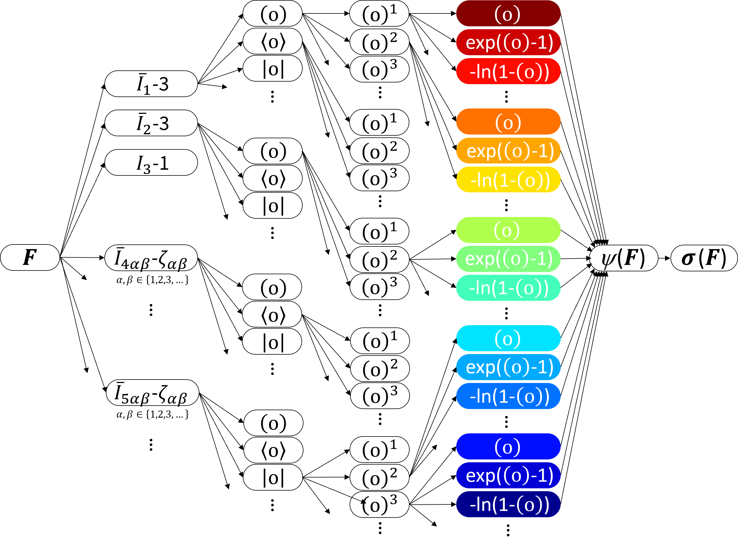
Figure 1: Constitutive neural network architecture. Anisotropic, compressible, feed forward constitutive neural network with three hidden layers to approximate the single scalar-valued free energy $\psi(\bar{I}_{1},\bar{I}_{2},I_{3},\bar{I}_{\rm{4\alpha\beta}},\bar{I}_{\rm{5\alpha\beta}})$, as a function of 15 invariants of the left Cauchy-Green deformation tensor $\bm{b}$. The zeroth layer generates identity $(\circ)$, the rectified linear unit $\langle\circ\rangle$, and the absolute value $\langle\circ\rangle$ of the 15 invariants. The first layer generates powers $(\circ)$, $(\circ)^{2}$, $(\circ)^{3}$, etc. and the second layer applies the identity $(\circ)$, the exponential $(\rm{exp}(\circ)-1)$, and the logarithm $(-\rm{ln}(1-(\circ)))$ to these powers. The network is not fully connected by design to satisfy the condition of polyconvexity a priori.

2.1 Kinematics

We introduce the deformation map $\bm{\varphi}$ as the mapping of material points $\bm{X}$ in the undeformed configuration to points $\bm{x}=\bm{\varphi}(\bm{X})$ in the deformed configuration [4, 39]. The gradient of the deformation map $\bm{\varphi}$ with respect to the undeformed coordinates $\bm{X}$ defines the deformation gradient $\bm{F}$ with its determinant $J$,

$$\bm{F}=\nabla_{{\rm{\bf{X}}}{}}\bm{\varphi}\quad\mbox{with}\quad J=\det(\bm{F})>0,$$ (1)

We multiplicatively decompose the deformation gradient $\bm{F}$ into its volumetric $\bm{F}^{\rm{vol}}$ and isochoric $\bar{\bm{F}}$ parts [25],

$$\bm{F}=\bm{F}^{\rm{vol}}\cdot\bar{\bm{F}}\quad\mbox{with}\quad\bm{F}^{\rm{vol}}=J^{\frac{1}{3}}\bm{I}\quad\mbox{and}\quad\bar{\bm{F}}=J^{-\frac{1}{3}}\bm{F}.$$ (2)

As deformation measures, we introduce the left and right Cauchy-Green deformation tensors, $\bm{b}$ and $\bm{C}$, and their isochoric counterparts, $\bar{\bm{b}}$ and $\bar{\bm{C}}$,

$$\begin{array}[]{l@{}c@{}l@{}c@{}l}\bm{b}&=&\bm{F}^{{\rm{t}}{}}&\cdot&\bm{F}\\ \bm{C}&=&\bm{F}&\cdot&\bm{F}^{{\rm{t}}{}}\end{array}\qquad\mbox{and}\qquad\begin{array}[]{l@{}c@{}l@{}c@{}l}\bar{\bm{b}}&=&\bar{\bm{F}}^{{\rm{t}}{}}&\cdot&\bar{\bm{F}}\\ \bar{\bm{C}}&=&\bar{\bm{F}}&\cdot&\bar{\bm{F}}^{{\rm{t}}{}}\,.\end{array}$$ (3)

We further assume directionally-dependent behavior, with three preferred directions, $\bm{n}_{1}^{0}$, $\bm{n}_{2}^{0}$, $\bm{n}_{3}^{0}$, associated with the material’s internal fiber directions in the reference configuration, where all three vectors are unit vectors, $||\,\bm{n}_{1}^{0}\,||=1$, $||\,\bm{n}_{2}^{0}\,||=1$, $||\,\bm{n}_{3}^{0}\,||=1$. Based on the volumetric and isochoric decomposition, and the underlying fiber orientations in the material, we characterize the deformation in terms of 15 invariants [96, 69]. More specifically, we define one isotropic volumetric invariant,

$$I_{3}=\det(\bm{F}^{{\rm{t}}{}}\cdot\bm{F})=J^{2}\,,$$ (4)

two isotropic deviatoric invariants,

$$\bar{I}_{1}=[\bar{\bm{F}}^{{\rm{t}}{}}\cdot\bar{\bm{F}}]:\bm{I}$$ (5)

$$\bar{I}_{2}=\mbox{$\frac{1}{2}$}\;[\bar{I}_{1}^{2}-[\bar{\bm{F}}^{{\rm{t}}{}}\cdot\bar{\bm{F}}]:[\bar{\bm{F}}^{{\rm{t}}{}}\cdot\bar{\bm{F}}]],$$

six anisotropic deviatoric invariants,

$$\begin{array}[]{l@{\hspace*{0.4cm}}l}\bar{I}_{\rm{4(11)}}=[\bar{\bm{F}}^{{\rm{t}}{}}\cdot\bar{\bm{F}}]:[\bm{n}_{1}^{0}\otimes\bm{n}_{1}^{0}]\hfil\hskip 11.38092pt&\bar{I}_{\rm{5(11)}}=[\bar{\bm{F}}^{{\rm{t}}{}}\cdot\bar{\bm{F}}]^{2}:[\bm{n}_{1}^{0}\otimes\bm{n}_{1}^{0}]\\ \bar{I}_{\rm{4(22)}}=[\bar{\bm{F}}^{{\rm{t}}{}}\cdot\bar{\bm{F}}]:[\bm{n}_{2}^{0}\otimes\bm{n}_{2}^{0}]\hfil\hskip 11.38092pt&\bar{I}_{\rm{5(22)}}=[\bar{\bm{F}}^{{\rm{t}}{}}\cdot\bar{\bm{F}}]^{2}:[\bm{n}_{2}^{0}\otimes\bm{n}_{2}^{0}]\\ \bar{I}_{\rm{4(33)}}=[\bar{\bm{F}}^{{\rm{t}}{}}\cdot\bar{\bm{F}}]:[\bm{n}_{3}^{0}\otimes\bm{n}_{3}^{0}]\hfil\hskip 11.38092pt&\bar{I}_{\rm{5(33)}}=[\bar{\bm{F}}^{{\rm{t}}{}}\cdot\bar{\bm{F}}]^{2}:[\bm{n}_{3}^{0}\otimes\bm{n}_{3}^{0}]\end{array}$$ (6)

and six deviatoric coupling invariants,

$$\begin{array}[]{l@{\hspace*{0.4cm}}l}\bar{I}_{\rm{4(12)}}=[\bar{\bm{F}}^{{\rm{t}}{}}\cdot\bar{\bm{F}}]:[\bm{n}_{1}^{0}\otimes\bm{n}_{2}^{0}]\hfil\hskip 11.38092pt&\bar{I}_{\rm{5(12)}}=[\bar{\bm{F}}^{{\rm{t}}{}}\cdot\bar{\bm{F}}]^{2}:[\bm{n}_{1}^{0}\otimes\bm{n}_{2}^{0}]\\ \bar{I}_{\rm{4(13)}}=[\bar{\bm{F}}^{{\rm{t}}{}}\cdot\bar{\bm{F}}]:[\bm{n}_{1}^{0}\otimes\bm{n}_{3}^{0}]\hfil\hskip 11.38092pt&\bar{I}_{\rm{5(13)}}=[\bar{\bm{F}}^{{\rm{t}}{}}\cdot\bar{\bm{F}}]^{2}:[\bm{n}_{1}^{0}\otimes\bm{n}_{3}^{0}]\\ \bar{I}_{\rm{4(23)}}=[\bar{\bm{F}}^{{\rm{t}}{}}\cdot\bar{\bm{F}}]:[\bm{n}_{2}^{0}\otimes\bm{n}_{3}^{0}]\hfil\hskip 11.38092pt&\bar{I}_{\rm{5(23)}}=[\bar{\bm{F}}^{{\rm{t}}{}}\cdot\bar{\bm{F}}]^{2}:[\bm{n}_{2}^{0}\otimes\bm{n}_{3}^{0}]\end{array}$$ (7)

Note that these coupling invariants reverse their sign if one of the fiber directions changes its sign, and can therefore not be considered strictly invariant. Nevertheless, these pseudo-invariants were found to be convenient for the definition of anisotropic constitutive models [42].

2.2 Free energy function

To ensure thermodynamic consistency, we introduce the Helmholtz free energy $\psi$ as a function of the deformation gradient $\psi=\psi\left(\bm{F}\right)$. Assuming no dissipative energy losses within the material, and rewriting the Clausius–Duhem entropy inequality [85] following the Coleman and Noll principle [12, 29], we derive

$$\bm{\sigma}=\frac{1}{J}\frac{\partial\psi\left(\bm{F}\right)}{\partial\bm{F}}\cdot\bm{F}^{\rm{t}}{}$$ (8)

as the constitutive relation between Cauchy stress $\bm{\sigma}$ and deformation gradient $\bm{F}$. To guarantee that our free energy function $\psi$ satisfies material objectivity and material symmetry, we further constrain our stress responses to be functions of the invariants of the left and right Cauchy Green deformation tensors $\bm{b}$ and $\bm{C}$ [96, 97]. This results in the general definition of the free energy function $\psi$ as a function of the 15 invariants,

$$\psi\left(\bm{F}\right)\doteq\psi\left(\bar{I}_{1}\,,\bar{I}_{2}\,,I_{3}\,,\bar{I}_{\rm{4(\alpha\beta)}}\,,\bar{I}_{\rm{5(\alpha\beta)}}\right),$$ (9)

with $\alpha\,,\beta\in\{1,2,3\}$ and $\beta\geq\alpha$. To account for the quasi-incompressible behavior of soft materials, we make the constitutive choice to additively decompose our free energy function $\psi$ into volumetric $\psi^{\rm{vol}}$ and isochoric $\bar{\psi}$ parts,

$$\psi\doteq\psi^{\rm{vol}}+\bar{\psi}.$$ (10)

Here, we define the volumetric free energy contribution,

$$\psi^{\rm{vol}}=\psi_{3}(I_{3})\,,$$ (11)

in terms of the isotropic volumetric invariant $I_{3}$ (Eq. 4), and the deviatoric free energy contribution,

$$\bar{\psi}=\bar{\psi}\left(\bar{I}_{1}\,,\bar{I}_{2}\,,\bar{I}_{\rm{4(\alpha\beta)}}\,,\bar{I}_{\rm{5(\alpha\beta)}}\right),$$ (12)

as functions of the isotropic and anisotropic deviatoric invariants from Eqs. 5 and 6, with $\alpha\,,\beta\in\{1,2,3\}$ and $\beta\geq\alpha$.

2.3 Constitutive neural network

With the aim to universally model a hyperelastic history-independent soft matter material behavior, we design a modular constitutive neural network architecture depicted in Figure 1. Leveraging our prior work on automated constitutive model discovery for isotropic [60, 61, 82], transversely isotropic [59, 81], and orthotropic [64] soft materials, we create a universal function approximator, which maps the 15 invariants $\bar{I}_{1}$, $\bar{I}_{2}$, $I_{3}$, $\bar{I}_{\rm{4(\alpha\beta)}}$, $\bar{I}_{\rm{5(\alpha\beta)}}$ of the deformation gradient $\bm{F}$ onto the free energy function $\psi\left(\bm{F}\right)$. The constitutive relation between the Cauchy stress $\bm{\sigma}$ and the deformation gradient $\bm{F}$ follows naturally from the second law of thermodynamics as the derivative of the free energy function $\psi$ with respect to the deformation gradient $F$ according to Eq. 8. We ensure a vanishing free energy $\psi\left(\bm{F}\right)\doteq 0$ in the reference configuration, i.e., when $\bm{F}=\bm{I}$, by using the invariants’ deviation from the energy-free reference state, $[\bar{I}_{1}-3]$, $[\bar{I}_{2}-3]$, $[I_{3}-1]$, $[\bar{I}_{\rm{4(\alpha\beta)}}-\zeta_{\alpha\beta}]$, $[\bar{I}_{\rm{5(\alpha\beta)}}-\zeta_{\alpha\beta}]$, as constitutive neural network input. Here, $\zeta_{\alpha\beta}=\bm{n}_{\alpha}^{0}\cdot\bm{n}_{\beta}^{0}$ corrects invariants $\bar{I}_{\rm{4(\alpha\beta)}}$ and $\bar{I}_{\rm{5(\alpha\beta)}}$ for their values in the undeformed configuration. This correction a priori ensures a stress-free reference configuration. To ensure polyconvexity, we design the constitutive neural network architecture as a locally connected, rather than a fully connected, feed forward neural network. Specifically, we design the free energy function as a sum of individual polyconvex subfunctions with respect to each of the individual contributing invariants. As a result, our free energy function from Eqs. 9-12 can be additively decomposed into

$$\psi= \bar{\psi}_{1}(\bar{I}_{1})+\bar{\psi}_{2}(\bar{I}_{2})+\psi_{3}({I}_{3})+$$ (13)

$$\sum_{\alpha=1}^{N}\sum_{\beta=\alpha}^{N}\bar{\psi}_{\rm{4\left(\alpha\beta\right)}}\left(\bar{I}_{\rm{4\left(\alpha\beta\right)}}\right)+\sum_{\alpha=1}^{N}\sum_{\beta=\alpha}^{N}\bar{\psi}_{\rm{5\left(\alpha\beta\right)}}\left(\bar{I}_{\rm{5\left(\alpha\beta\right)}}\right),$$

with $\alpha\,,\beta\in\{1,2,3\}$ and $\beta\geq\alpha$. Following Eq. 8, we derive the Cauchy stress

$$J\,\bm{\sigma} =2\frac{\partial\bar{\psi}_{1}}{\partial\bar{I}_{1}}\,\bar{\bm{b}}+2\frac{\partial\bar{\psi}_{2}}{\partial\bar{I}_{2}}\,[\bar{I}_{1}\bar{\bm{b}}-\bar{\bm{b}}^{2}]+2\frac{\partial\psi_{3}}{\partial{I}_{3}}\,I_{3}\bm{I}$$ (14)

$$+\sum_{\alpha=1}^{N}\sum_{\beta=\alpha}^{N}\frac{\partial\bar{\psi}_{\rm{4(\alpha\beta)}}}{\partial\bar{I}_{\rm{4(\alpha\beta)}}}\,\left[\bar{\bm{n}}_{\alpha}\otimes\bar{\bm{n}}_{\beta}+\bar{\bm{n}}_{\beta}\otimes\bar{\bm{n}}_{\alpha}\right]$$

$$+\sum_{\alpha=1}^{N}\sum_{\beta=\alpha}^{N}\frac{\partial\bar{\psi}_{\rm{5(\alpha\beta)}}}{\partial\bar{I}_{\rm{5(\alpha\beta)}}}\,\left[\bar{\bm{n}}_{\alpha}\otimes\bar{\bm{b}}\bar{\bm{n}}_{\beta}+\bar{\bm{b}}\bar{\bm{n}}_{\alpha}\otimes\bar{\bm{n}}_{\beta}\right.$$

$$\hskip 79.6678pt+\left.\bar{\bm{n}}_{\beta}\otimes\bar{\bm{b}}\bar{\bm{n}}_{\alpha}+\bar{\bm{b}}\bar{\bm{n}}_{\beta}\otimes\bar{\bm{n}}_{\beta}\right],$$

where $\bar{\bm{n}}_{\alpha}=\bar{\bm{F}}\cdot\bm{n}_{\alpha}^{0}$ and $\bar{\bm{n}}_{\beta}=\bar{\bm{F}}\cdot\bm{n}_{\beta}^{0}$ represent the deviatoric fiber vectors in the current configuration.
Our constitutive network consists of three hidden layers with activation functions that are custom-designed to satisfy physically reasonable constitutive restrictions [4, 60]. Specifically, we select from the identity $(\circ)$, the rectified linear unit function $\langle\circ\rangle$, and the modulus function $|\circ|$ for the zeroth layer of the network, from linear $(\circ)$, quadratic $(\circ)^{2}$, cubic $(\circ)^{3}$, and higher order powers for the first layer, and from linear $(\circ)$, exponential $\exp(\circ)$, and logarithmic $\ln(\circ)$ for the second layer.

3 A universal material model

We incorporate our universal material model within a finite element analysis environment. Specifically, we develop a user-defined material model subroutine which functionally maps the local deformation gradient $\bm{F}$ onto the free energy function $\psi$ and computes its derivative with respect to the deformation gradient $\bm{F}$ and the Cauchy stress tensor $\bm{\sigma}$ using Eq. 8. Additionally, we compute the stiffness tensor $\mathbb{C}$ to improve the accuracy, stability, and efficiency of the iterative solution technique required for an accurate prediction of the non-linear material behavior under various loading conditions.

3.1 Subroutine

To predict the quasi-static response of a system undergoing mechanical loading a non-linear finite element analysis solver iteratively evaluates whether a proposed update to the nodal displacement field satisfies the equilibrium equations that describe the force and momentum balance within the computational domain. This evaluation requires the computation of the stress tensor and the tangent stiffness tensor as functions of the proposed update to the body’s total deformation. At each time step, at each Newton-Raphson iteration, within each element, and for each integration point, the solver evaluates the constitutive response that characterizes the functional mapping between the deformation gradient $\bm{F}$ and the stress tensor $\bm{\sigma}$ and tangent stiffness tensor $\mathbb{C}$.

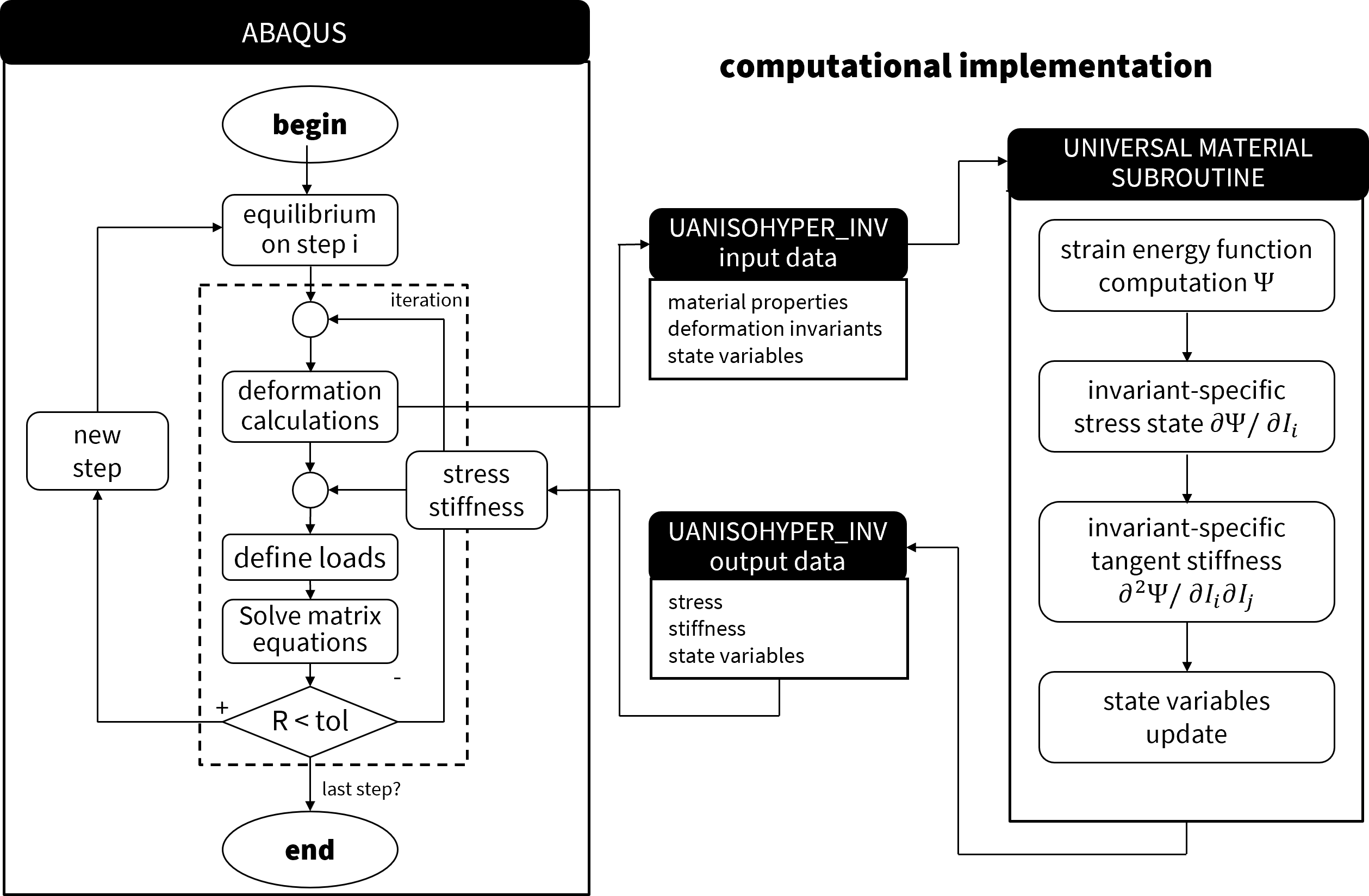
Figure 2: Interaction between the finite element analysis solver and the universal material subroutine. Flowchart of the interaction between Abaqus and the UANISOHYPER_INV subroutine architecture which embeds our universal constitutive material model. During each Newton-Raphson iteration and at each Gauss integration point, the UANISOHYPER_INV subroutine computes the strain energy function $\psi$, its first derivatives with respect to the deformation invariants ${\partial\psi}/{\partial\bar{I}_{i}}$, and its second derivatives with respect to the deformation invariants ${\partial^{2}\psi}/{\partial\bar{I}_{i}\partial\bar{I}_{j}}$. These quantities are used by Abaqus to compute the components of the Cauchy stress tensor and the material tangent stiffness tensor, to construct the element force vector and stiffness matrix, and to assemble the global righthand side vector and stiffness matrix. Abaqus then performs a Newton-Raphson iteration based on the residual between the internal and external forces, until it achieves convergence.

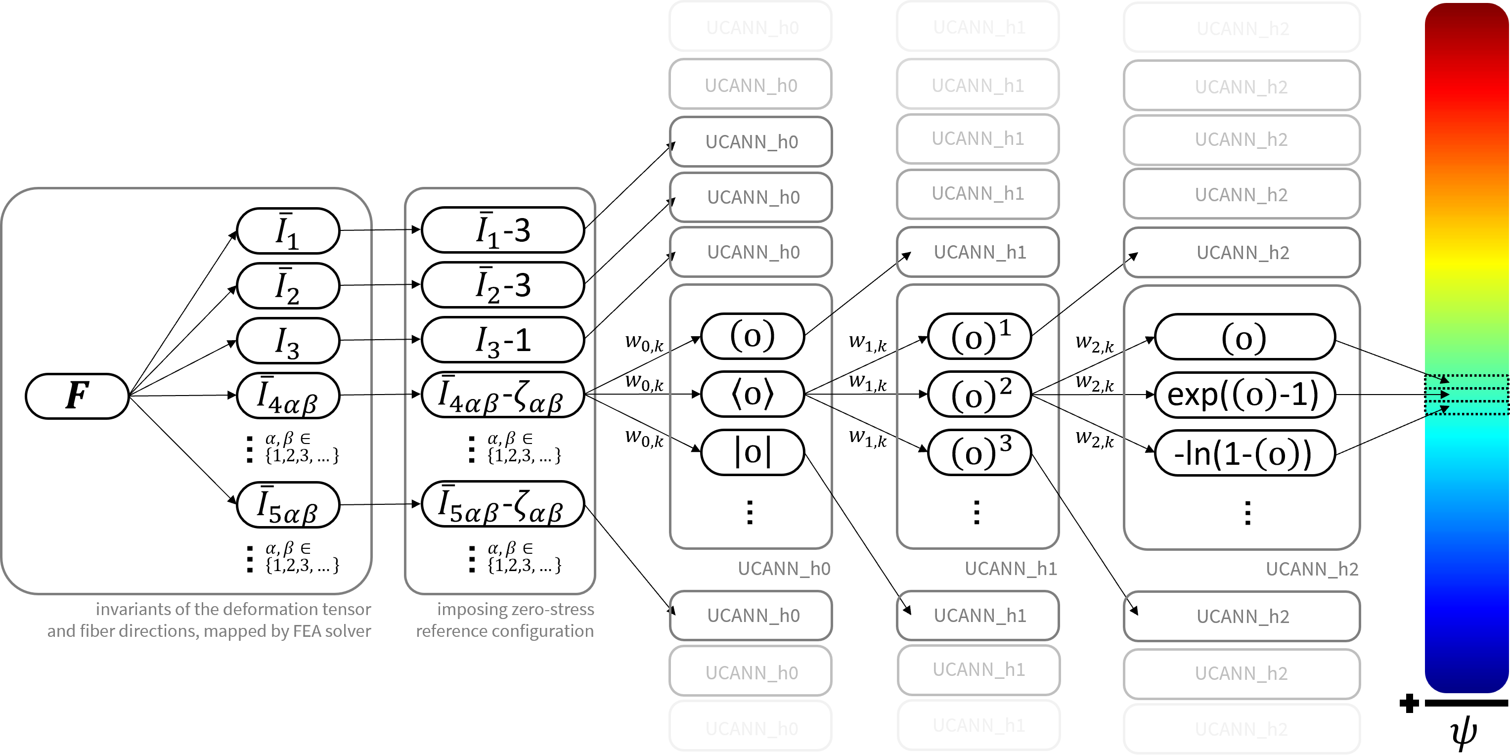
Figure 3: Universal material model subroutine schematic. Our universal material model user subroutine computes the strain energy function $\psi$ (= UA(1)), its first derivatives ${\partial\psi}/{\partial I_{i}}$ (= UI1(NINV)), and its second derivatives ${\partial^{2}\psi}/{\partial\bar{I}_{i}\partial\bar{I}_{j}}$ (=UI2(NINV^∗(NINV+1)/2)) with respect to the scalar invariants $\bar{I}_{i}$, derived from the deformation gradient $\bm{F}$. These functions and derivatives are computed based on a triple set of nested activation functions $f_{0}$ (= UCANN_h0), $f_{1}$ (= UCANN_h1), and $f_{2}$ (= UCANN_h2), where each unique constitutive path forms an additive constitutive neuron towards the total free energy and its derivatives.

We leverage the UANISOHYPER_INV user-defined subroutine architecture in Figure 2 to seamlessly integrate our universal constitutive neural network architecture within the Abaqus finite element analysis software suite [15]. This subroutine provides three input arrays: the material properties we provide in the finite element analysis input file; the deformation gradient invariants as defined in Eqs. 4,5,6, and 7; and an array of state-dependent field variables. Upon each evaluation, our user-defined subroutine updates the free energy function UA(1) $=\psi$, the array of first derivatives of the free energy with respect to the scalar invariants UI1(NINV) $={\partial\psi}/{\partial\bar{I}_{i}}$, and the array of second derivatives of the free energy with respect to the scalar invariants UI2(NINV^∗(NINV+1)/2)$={\partial^{2}\psi}/{\partial\bar{I}_{i}\partial\bar{I}_{j}}$.
Figure 3 showcases the internal code structure of our universal material model subroutine. We construct a triple set of nested activation functions UCANN_h0, UCANN_h1, and UCANN_h2 to compute $\psi$, ${\partial\psi}/{\partial\bar{I}_{i}}$, ${\partial^{2}\psi}/{\partial\bar{I}_{i}\partial\bar{I}_{j}}$ from $\bar{I}_{i}$. We adopt the invariant numbering,

$$\begin{array}[]{lcl}\bar{I}_{1}&\rightarrow&\bar{I}_{\texttt{NINV}};\;\texttt{NINV}=1\\ \bar{I}_{2}&\rightarrow&\bar{I}_{\texttt{NINV}};\;\texttt{NINV}=2\\ I_{3}&\rightarrow&I_{\texttt{NINV}};\;\texttt{NINV}=3\\ \bar{I}_{4(\alpha\beta)}&\rightarrow&\bar{I}_{\texttt{NINV}};\;\texttt{NINV}=4+2\,(\alpha-1)+\beta\,(\beta-1))\\ \bar{I}_{5(\alpha\beta)}&\rightarrow&\bar{I}_{\texttt{NINV}};\;\texttt{NINV}=5+2\,(\alpha-1)+\beta\,(\beta-1))\end{array}$$ (15)

Dependent on the number of fiber families, this scheme automatically adapts itself to account for multiple fiber orientations. For example, when our material displays an anisotropic behavior with three families of fibers (${\tt{NDIR}=3}$), there are a total of 15 invariants: $\bar{I}_{1}$, $\bar{I}_{2}$, $I_{3}=J$, six invariants of type $\bar{I}_{4(\alpha\beta)}$, and six invariants of type $\bar{I}_{5(\alpha\beta)}$, with $\alpha\,,\beta\in\{1,2,3\}$ and $\beta\geq\alpha$.

Free energy function update.

Without loss of generality, we reformulate the free energy $\psi$ from Eq. 13 in the following form,

$$\psi =f_{2}\circ f_{1}\circ f_{0}\,(\bar{I}_{i}-\bar{I}_{i0})$$ (16)

$$=\sum_{k=1}^{n}w_{2,k}\,f_{2,k}\,(f_{1,k}\,(f_{0,k}\,(\bar{I}_{i,k}-\bar{I}_{i0,k});w_{1,k}))\,,$$

where $f_{0}$, $f_{1}$, $f_{2}$ are the nested activation functions associated with the zeroth, first, and second layers of our constitutive neural network; $k=1,...,n$ defines each unique additive constitutive neuron that stems from the expanding nested constitutive neural network in Figure 3; and $\bar{I}_{i0}$ imposes the free energy $\psi$ and Cauchy stress $\bm{\sigma}$ to be zero in the reference configuration. As discussed above and shown in Figure 1, these corrections amount to $\bar{I}_{i0}=3$ for $i=1,2$, to $I_{i0}=1$ for $i=3$, and $\bar{I}_{i0}=\zeta_{\alpha\beta}=\bm{n}_{\alpha}^{0}\cdot\bm{n}_{\beta}^{0}$ for $i\geq 4$ with respect to the invariant numbering scheme in Eq. 15. Our nested activation functions in Eq. 22 read

$$f_{0}=\left\{\begin{array}[]{c}{\left(\circ\right)}\\ {\langle\circ\rangle}\\ {\lvert\circ\rvert}\\ \vdots\end{array}\right.\;f_{1}=\left\{\begin{array}[]{c}{(\circ)^{1}}\\ {(\circ)^{2}}\\ {(\circ)^{3}}\\ \vdots\\ {(\circ)^{m}}\end{array}\right.\;f_{2}=\left\{\begin{array}[]{c}{w_{1}\,(\circ)}\\ {{\rm{exp}}(w_{1}\,(\circ))-1}\\ -{{\rm{ln}}(1-w_{1}\,(\circ))}\\ \vdots\end{array}\right.\!\!.$$ (17)

The activation function $f_{0}$ returns the identity, Macauley bracketed, or absolute values, $(\circ)$, $\langle\circ\rangle$, $\lvert\circ\rvert$ of the zero-stress reference configuration corrected invariants; $f_{1}$ raises these invariants to the first, second, third, or any higher order powers, $(\circ)^{1}$, $(\circ)^{2}$, $(\circ)^{3}$, $(\circ)^{m}$; and $f_{2}$ applies the identity, exponential, or natural logarithm, $(\circ)$, $(\rm{exp}(\circ)-1)$, $(-\rm{ln}(1-(\circ)))$, or any other thermodynamically admissible function to these powers.

Cauchy stress tensor update.

To update the Cauchy stress tensor $\bm{\sigma}$, we reformulate Eq. 8 in the following form,

$$\bm{\sigma} =\frac{1}{J}\frac{\partial\psi\left(\bm{F}\right)}{\partial\bm{F}}\cdot\bm{F}^{{\rm{t}}{}}=\sum_{k=1}^{n}\frac{1}{J}\frac{\partial\psi}{\partial\bar{I}_{i,k}}\frac{\partial\bar{I}_{i,k}}{\partial\bm{F}}\cdot\bm{F}^{{\rm{t}}{}}$$ (18)

$$=\sum_{i}\frac{1}{J}\left(\sum_{k}^{n_{i}}\frac{\partial\psi}{\partial\bar{I}_{i,k}}\right)\frac{\partial\bar{I}_{i}}{\partial\bm{F}}\cdot\bm{F}^{{\rm{t}}{}}=\sum_{i}\frac{1}{J}\frac{\partial\psi}{\partial\bar{I}_{i}}\frac{\partial\bar{I}_{i}}{\partial\bm{F}}\cdot\bm{F}^{{\rm{t}}{}}$$

where Abaqus internally computes of the ${\partial\bar{I}_{i}}/{\partial\bm{F}}$ terms and the summation of the individual NINV stress tensor contributions. We compute all the invariant-specific scalar UI1(NINV) $={\partial\psi}/{\partial\bar{I}_{i}}$ contributions to the full UI1 array in our user subroutine,

$$\frac{\partial\psi}{\partial\bar{I}_{i}}=\sum_{k}^{n_{i}}\frac{\partial\psi}{\partial\bar{I}_{i,k}}=\sum_{k}^{n_{i}}w_{2,\mathrm{k}}\frac{\partial f_{2,k}}{\partial(\circ)}\frac{\partial f_{1,k}}{\partial(\circ)}\frac{\partial f_{0,k}}{\partial\bar{I}_{i,k}}$$ (19)

in terms of the first derivatives of our activation functions

$$\frac{\partial f_{0}}{\partial(\circ)}=\left\{\begin{array}[]{@{\hspace*{0.0cm}}c}1\\ \frac{\frac{\lvert\circ\rvert}{\circ}+1}{2}\\ \frac{\lvert\circ\rvert}{\circ}\\ \vdots\end{array}\right.\frac{\partial f_{1}}{\partial(\circ)}=\left\{\begin{array}[]{@{\hspace*{0.0cm}}c}{1(\circ)^{0}}\\ {2(\circ)^{1}}\\ {3(\circ)^{2}}\\ \vdots\\ m(\circ)^{m-1}\end{array}\right.\!\!\frac{\partial f_{2}}{\partial(\circ)}=\left\{\begin{array}[]{@{\hspace*{0.0cm}}c}{w_{1}}\\ {w_{1}{\rm{exp}}(w_{1}(\circ))}\\ {w_{1}/(1\mbox{-}w_{1}(\circ))}\\ \vdots\end{array}\right.$$ (20)

Tangent stiffness tensor update.

To internally compute the tangent stiffness tensor, Abaqus needs the second derivatives of the strain energy function with respect to the invariants ${\partial^{2}\Psi}/{\partial\bar{I}_{i,k}\partial\bar{I}_{j,k}}$. Here, given the nested structure of our universal material model subroutine, we have ${\partial^{2}\Psi}/{\partial\bar{I}_{i,k}\partial\bar{I}_{j,k}}=0$ , when $i\neq j$ As such, we only have non-zero values

$$\frac{\partial^{2}\Psi}{\partial\bar{I}_{i,k}^{2}}=\sum_{k=1}^{n_{i}}w_{2,k} \left[\left(\frac{\partial^{2}f_{2,k}}{\partial(\circ)^{2}}\left[\frac{\partial f_{1,k}}{\partial(\circ)}\right]^{2}+\frac{\partial f_{2,k}}{\partial(\circ)}\frac{\partial^{2}f_{1,k}}{\partial(\circ)^{2}}\right)\right.$$ (21)

$$\left.\hskip 11.38092pt\left[\frac{\partial f_{0,k}}{\partial\bar{I}_{i,k}}\right]^{2}+\frac{\partial f_{2,k}}{\partial(\circ)}\frac{\partial f_{1,k}}{\partial(\circ)}\frac{\partial^{2}f_{0,k}}{\partial\bar{I}_{i,k}^{2}}\right]$$

in terms of the second derivatives of our activation functions,

$$\begin{array}[]{l@{\hspace{-0.2cm}}l}\displaystyle{\frac{\partial^{2}f_{1}}{\partial\left(\circ\right)^{2}}}=\left\{\begin{array}[]{c}0\\ 2\\ 6\\ \vdots\\ (m^{2}-m)(\circ)^{m-2}\end{array}\right.&\displaystyle{\frac{\partial^{2}f_{2}}{\partial\left(\circ\right)^{2}}}=\left\{\begin{array}[]{c}0\\ {{w_{1}}^{2}{\rm{exp}}(w_{1}(\circ))}\\ {{w_{1}}^{2}/{(1-w1(\circ))^{2}}}\\ \vdots\end{array}\right.\end{array}$$ (22)

where the second derivative of the zeroth layer functions, $\partial^{2}f_{0}/\partial(\circ)^{2}$, vanishes identically for all three terms.

3.2 Pseudocodes

In the following five algorithmic boxes, we summarize our universal material subroutine as pseudocode.

subroutine UANISOHYPER_INV(aInv,UA,UI1,UI2)

       // initialize variables

       set initial array values for UA, UI1, UI2;

       set reference configuration UANISOHYPER_INV;

       set discovered parameters UNIVERSAL_TAB;

       // evaluate all n rows in parameter table

       for k in n do

             // invariant, activation functions, weights

             extract invariant kf0(k);

             extract activation functions kf1(k), kf2(k); extract weights w1(k), w2(k);

             // invariant in reference configuration

             xInv = aInv(kf0(k))-xInv0(k);

             // energy and derivatives UA, UI1, UI2

             call uCANN(xInv,kf1(k),kf2(k),w1(k),                w2(k),UA,UI1,UI2);

       end for

      // return updated arrays

       return UA, UI1, UI2

Algorithm 1 Pseudocode for universal material subroutine UANISOHYPER_INV

subroutine uCANN(xInv,kf1,kf2,w1,w2,UA,UI1,UI2)

       // zeroth layer: calculate f0,df0,ddf0

       call uCANN_h0(xInv,kf0,f0,df0,ddf0);

       // first layer: calculate f1,df1,ddf1

       w0 = 1;

       call uCANN_h1(xInv,w0,kf1,f1,df1,ddf1);

       // second layer: calculate f2,df2,ddf2

       call uCANN_h2(f1,w1,kf2,f2,df2,ddf2);

       // update energy and derivatives UA,UI1,UI2

       UA   = UA   + w2 * f2;

       UI1 = UI1 + w2 * df2*df1*df0;

       UI2 = UI2 + w2 *((ddf2*df1**2+df2*ddf1)                         *df0**2+df2*df1*ddf0);

       return UA, UI1, UI2

Algorithm 2 Pseudocode to update energy and its derivatives UA, UI1, UI2

subroutine uCANN_h0(x,kf,f,df,ddf)

       // calculate zero layer output f,df,ddf for activation function kf

       if  kf = 1  then

             f = x;

             df = 1;

             ddf = 0;

            

       else if kf = 2 then

             f = $(\lvert x\rvert+x)/2$;

             df = $(\lvert x\rvert/x+1)/2$;

             ddf = 0;

            

       else if kf = 3 then

             f = $\lvert x\rvert$;

             df = $\lvert x\rvert/x$;

             ddf = 0;

            

       return f,df,ddf

Algorithm 3 Pseudocode to evaluate output of zeroth network layer f,df,ddf

subroutine uCANN_h1(x,w,kf,f,df,ddf)

       // calculate first layer output f,df,ddf for activation function kf

       if  kf = 1  then

             f = w * x;

             df = w * 1;

             ddf = w * 0;

            

       else if kf = 2 then

             f = w**2 * x**2;

             df = w**2 * 2*x;

             ddf = w**2 * 2;

            

       return f,df,ddf

Algorithm 4 Pseudocode to evaluate output of first network layer f,df,ddf

subroutine uCANN_h2(x,kf,w,f,df,ddf)

       // calculate second layer output f,df,ddf for activation function kf

       if  kf = 1  then

             f = w * x;

             df = w * 1;

             ddf = w * 0;

            

       else if  kf = 2  then

             f = exp(w*x)-1;

             df = w * exp(w*x);

             ddf = w**2 * exp(w*x);

            

       else if  kf = 3  then

             f = -ln(1-w*x);

             df = w / (1-w*x);

             ddf = w**2 / (1-w*x)**2;

            

       return f,df,ddf

Algorithm 5 Pseudocode to evaluate output of second network layer f,df,ddf

Algorithm 1 illustrates the UANISOHYPER_INV pseudocode to compute the arrays UA(1), UI1(NINV), and UI2(NINV ^∗(NINV+1)/2) at the integration point level. First, we initialize all relevant arrays and read the activation functions $kf_{0,k}$, $kf_{1,k}$ and $kf_{2,k}$ and weights $w_{0,k}$, $w_{1,k}$ and $w_{2,k}$ of the $n$ constitutive neurons of our constitutive neural network from our user-defined parameter table UNIVERSAL_TAB, where $w_{0,k}=1.0$ by default. Then, for each node, we evaluate its row in the parameter table UNIVERSAL_TAB and additively update the strain energy density function and its first and second derivatives, UA, UI1, UI2.
Algorithm 2 summarizes the additive update of the free energy and its first and second derivatives, UA, UI1, UI2, within the universal material subroutine uCANN.
Algorithms 3,4 and 5 provide the pseudocode for the three subroutines uCANN_h0, uCANN_h1 and uCANN_h2 that evaluate the zeroth, first and second network layers for each network node with its discovered activation functions and weights.

3.3 FEA integration

The concept of our universal material subroutine is inherently modular and generally compatible with any finite element analysis package [15, 3, 62, 105, 2]. Here, for illustrative purposes, we implement the universal material subroutine in Abaqus FEA [15], and make all our code and simulation files publicly available on Zenodo. For the input file to our finite element simulation, we define our discovered model and parameters in a parameter table. Each row of this table represents a neuron of the final layer in our constitutive neural network and consists of seven terms: an integer kfinv that defines the index of the invariant $\bar{I}_{i}$ according to the invariant numbering scheme in equation 15; three integers kf0,kf1 and kf2 that define the indices of the zeroth-, first-, and second-layer activation functions; and three floats w0, w1 and w2 that define the weights of the zeroth, first, and second layers. In Abaqus, we declare the format of this input parameter table using the parameter table type definition in the UNIVERSAL_PARAM_TYPES.INC file.
$\begin{array}[]{@{}l}\mbox{{\bf{\tt{*PARAMETER TABLE TYPE, name="UNIVERSAL\_TAB",}}}}\\ \hskip 5.69046pt\mbox{{\bf{\tt{parameters = 7}}}}\\ \begin{array}[]{lll}\mbox{\bf{\tt{INTEGER}}}\,,&\,\bf{\tt{,}}&\mbox{\bf{\tt{"index invariant, kfinv,o"}}}\\ \mbox{\bf{\tt{INTEGER\,,}}}&\,\bf{\tt{,}}&\mbox{\bf{\tt{"index 0th activ function, kf0,o"}}}\\ \mbox{\bf{\tt{INTEGER\,,}}}&\,\bf{\tt{,}}&\mbox{\bf{\tt{"index 1st activ function, kf1,o"}}}\\ \mbox{\bf{\tt{INTEGER\,,}}}&\,\bf{\tt{,}}&\mbox{\bf{\tt{"index 2nd activ function, kf2,o"}}}\\ \mbox{\bf{\tt{FLOAT\,,}}}&\,\bf{\tt{,}}&\mbox{\bf{\tt{"weight 0th hidden layer, w0,o"}}}\\ \mbox{\bf{\tt{FLOAT\,,}}}&\,\bf{\tt{,}}&\mbox{\bf{\tt{"weight 1st hidden layer, w1,o"}}}\\ \mbox{\bf{\tt{FLOAT\,,}}}&\,\bf{\tt{,}}&\mbox{\bf{\tt{"weight 2nd hidden layer, w2,o"}}}\\ \end{array}\end{array}$
Within our Abaqus FEA simulation input file, we include the parameter table type definition using
$\begin{array}[]{@{}l}\mbox{{\bf{\tt{*INCLUDE, INPUT=UNIVERSAL\_PARAM\_TYPES.INC}}}}\end{array}$
and call our user-defined material model through the command
$\begin{array}[]{@{}l}\mbox{{\bf{\tt{*ANISOTROPIC\;HYPERELASTIC,\,USER,\,FORMULATION=INVARIANT,}}}}\\ \hskip 4.26773pt\mbox{{\bf{\tt{TYPE=INCOMPRESSIBLE, LOCAL DIRECTIONS=NDIR}}}}\end{array}$
where integer NDIR defines the number of local fiber directions in our material, followed by the discovered list of parameters:
$\begin{array}[]{@{}l}\mbox{{\bf{\tt{*PARAMETER TABLE, TYPE="UNIVERSAL\_TAB"}}}}\\ \mbox{{\bf{\tt{1,1,1,1,1.0,w${}_{\tt{1,1}}$,w${}_{\tt{2,1}}$}}}}\\ \mbox{{\bf{\tt{1,1,1,2,1.0,w${}_{\tt{1,2}}$,w${}_{\tt{2,2}}$}}}}\\ \mbox{{\bf{\tt{1,1,2,1,1.0,w${}_{\tt{1,3}}$,w${}_{\tt{2,3}}$}}}}\\ \mbox{{\bf{$\vdots$}}}\end{array}$
The first index of each row selects between the invariants, the second index applies the identity, Macauley brackets, or absolute values to the invariants, $(\circ)$, $\langle\circ\rangle$, $\lvert\circ\rvert$, the third index raises them the first, second, third, or any higher order powers, $(\circ)^{1}$, $(\circ)^{2}$, and the fourth index applies the identity, exponential, or natural logarithm, $(\circ)$, $(\rm{exp}(\circ)-1)$, $(-\rm{ln}(1-(\circ)))$, or any other thermodynamically admissible function to these powers. For brevity, we can simply exclude terms with zero weights from the list.

3.4 Compressibility

To extend our universal material model subroutine towards compressible materials, we add a volumetric strain energy function $\psi_{\rm{vol}}$ in terms of the third invariant $I_{3}$. We follow the same nested activation function approach as in Figure 3, and add the volumetric strain energy density $\psi^{\rm{vol}}$, its first derivative ${\partial\psi^{\rm{vol}}}/{\partial I_{3}}$ and its second derivatives ${\partial^{2}\psi_{\rm{vol}}}/{\partial I_{3}^{2}}$ to the UA(1), UI1(NINV), UI2(NINV^∗(NINV+1)/2) arrays. Using the invariant numbering scheme from equation 15, we have NINV$=3$, and introduce UA(1), UI1(3) and UI2(6). To incorporate compressible material behavior in our FEA simulation, we change the TYPE keyword argument line in our Abaqus input file to TYPE = COMPRESSIBLE,
$\begin{array}[]{@{}l}\mbox{{\bf{\tt{*ANISOTROPIC\;HYPERELASTIC,\,USER,\,FORMULATION=INVARIANT,}}}}\\ \hskip 4.26773pt\mbox{{\bf{\tt{TYPE=COMPRESSIBLE, LOCAL DIRECTIONS=NDIR}}}}\end{array}$
where integer NDIR defines the number of local fiber directions of our material. We add the volumetric contributions to our constitutive parameter table, along with all the other deviatoric free energy contributions,
$\begin{array}[]{@{}l}\mbox{{\bf{\tt{*PARAMETER TABLE, TYPE="UNIVERSAL\_TAB"}}}}\\ \begin{array}[]{ttttttt}\vdots&\vdots&\vdots&\vdots&\vdots&\vdots&\vdots\\ 3,&1,&1,&1,&1.0,&w_{1,\circ},&w_{2,\circ}\\ 3,&1,&2,&1,&1.0,&w_{1,\circ},&w_{2,\circ}\end{array}\end{array}$
For example, the volumetric strain energy function [94]

$$\psi_{\mathrm{vol}}=\frac{K}{2}(I_{3}-1)^{2}$$ (23)

translates into the following contribution to the input file
$\begin{array}[]{@{}l}\mbox{{\bf{\tt{*PARAMETER TABLE, TYPE="UNIVERSAL\_TAB"}}}}\\ \mbox{{\bf{\tt{3,1,2,1,1.0,1.0,K/2}}}}\\ \end{array}$
Alternatively, the volumetric strain energy function

$$\psi_{\mathrm{vol}}=\frac{K}{2}\left(\frac{I_{3}^{2}-1}{2}-\ln(I_{3})\right)$$ (24)

which is a special case of the modified Ogden formulation [77], can be reformulated to

$$\psi_{\mathrm{vol}}=\frac{K}{2}\left(\!(I_{3}-1)+\frac{1}{2}(I_{3}-1)^{2}-\ln(1-(-1)(I_{3}-1))\!\right)$$ (25)

which translates into the following lines in the input file
$\begin{array}[]{@{}l}\mbox{{\bf{\tt{*PARAMETER TABLE, TYPE="UNIVERSAL\_TAB"}}}}\\ \begin{array}[]{ttttttt}3,&1,&1,&1,&1.0,&1.0,&K/2\\ 3,&1,&2,&1,&1.0,&0.5,&K/2\\ 3,&1,&1,&3,&1.0,&\text{-}1.0,&K/2\end{array}\end{array}$

3.5 The subroutine applied

To showcase the flexibility and modularity of our universal material model subroutine, we demonstrate how our approach naturally integrates the popular neo Hooke [104], Mooney Rivlin [71, 89], Yeoh [112], polynomial [88], Holzapfel [40], and Kaliske [47] models into Abaqus FEA. For each model, we provide the strain energy function and its translation into the UNIVERSAL_TAB parameter table for the FEA input file.

Neo Hooke model

The strain energy function of the compressible linear first invariant neo Hooke model [104]

$$\psi=C_{10}\left(\bar{I}_{1}-3\right)+\frac{1}{D_{1}}\left(I_{3}-1\right)^{2}$$ (26)

translates into the following two-line parameter table
$\begin{array}[]{@{}l}\mbox{{\bf{\tt{*PARAMETER TABLE, TYPE="UNIVERSAL\_TAB"}}}}\\ \begin{array}[]{ttttttt}1,&1,&1,&1,&1.0,&1.0,&C_{10}\\ 3,&1,&2,&1,&1.0,&1.0,&1/D_{1}\end{array}\end{array}$

Mooney Rivlin model

The strain energy function of the compressible linear first and second invariant Mooney Rivlin model [71, 89]

$$\psi=C_{10}\left(\bar{I}_{1}-3\right)+C_{01}\left(\bar{I}_{2}-3\right)+\frac{1}{D_{1}}\left(I_{3}-1\right)^{2}$$ (27)

translates into the following three-line parameter table
$\begin{array}[]{@{}l}\mbox{{\bf{\tt{*PARAMETER TABLE, TYPE="UNIVERSAL\_TAB"}}}}\\ \begin{array}[]{ttttttt}1,&1,&1,&1,&1.0,&1.0,&C_{10}\\ 2,&1,&1,&1,&1.0,&1.0,&C_{01}\\ 3,&1,&2,&1,&1.0,&1.0,&1/D_{1}\end{array}\end{array}$

Yeoh model

The strain energy function of the compressible first invariant Yeoh model [112]

$$\psi =C_{10}\left(\bar{I}_{1}-3\right)+C_{20}\left(\bar{I}_{1}-3\right)^{2}+C_{30}\left(\bar{I}_{1}-3\right)^{3}$$ (28)

$$+\frac{1}{D_{1}}\left(I_{3}-1\right)^{2}+\frac{1}{D_{2}}\left(I_{3}-1\right)^{4}+\frac{1}{D_{3}}\left(I_{3}-1\right)^{6}$$

translates into the following six-line parameter table
$\begin{array}[]{@{}l}\mbox{{\bf{\tt{*PARAMETER TABLE, TYPE="UNIVERSAL\_TAB"}}}}\\ \begin{array}[]{ttttttt}1,&1,&1,&1,&1.0,&1.0,&C_{10}\\ 1,&1,&2,&1,&1.0,&1.0,&C_{20}\\ 1,&1,&3,&1,&1.0,&1.0,&C_{30}\\ 3,&1,&2,&1,&1.0,&1.0,&1/D_{1}\\ 3,&1,&4,&1,&1.0,&1.0,&1/D_{2}\\ 3,&1,&6,&1,&1.0,&1.0,&1/D_{3}\\ \end{array}\end{array}$

Polynomial model

The strain energy function of the compressible first invariant polynomial model [88]

$$\psi=\sum_{i=1}^{N}C_{i0}\left(\bar{I}_{1}-3\right)^{i}+\sum_{i=1}^{N}\frac{1}{D_{i}}\left(I_{3}-1\right)^{2i}$$ (29)

translates into the following parameter table
$\begin{array}[]{@{}l}\mbox{{\bf{\tt{*PARAMETER TABLE, TYPE="UNIVERSAL\_TAB"}}}}\\ \begin{array}[]{ttttttt}1,&1,&1,&1,&1.0,&1.0,&C_{10}\\ 1,&1,&2,&1,&1.0,&1.0,&C_{20}\\ 1,&1,&3,&1,&1.0,&1.0,&C_{30}\\ \vdots&\vdots&\vdots&\vdots&\vdots&\vdots&\vdots\\ 1,&1,&N,&1,&1.0,&1.0,&C_{N0}\\ 3,&1,&2,&1,&1.0,&1.0,&1/D_{1}\\ 3,&1,&4,&1,&1.0,&1.0,&1/D_{2}\\ 3,&1,&6,&1,&1.0,&1.0,&1/D_{3}\\ \vdots&\vdots&\vdots&\vdots&\vdots&\vdots&\vdots\\ 3,&1,&N*2,&1,&1.0,&1.0,&1/D_{N}\\ \end{array}\end{array}$

Holzapfel model

The strain energy function of the compressible two-fiber family Holzapfel model [40]

$$\psi =C_{10}\left(\bar{I}_{1}-3\right)+\frac{1}{D}\left(\frac{I_{3}^{2}-1}{2}-\ln{I_{3}}\right)$$ (30)

$$+\frac{k_{1}}{2k_{2}}\left(\exp{\left[k_{2}\langle\bar{I}_{4(11)}-1\rangle^{2}\right]}-1\right)$$

$$+\frac{k_{1}}{2k_{2}}\left(\exp{\left[k_{2}\langle\bar{I}_{4(22)}-1\rangle^{2}\right]}-1\right)$$

translates into the following six-line parameter table
$\begin{array}[]{@{}l}\mbox{{\bf{\tt{*PARAMETER TABLE, TYPE="UNIVERSAL\_TAB"}}}}\\ \begin{array}[]{ttttttt}1,&1,&1,&1,&1.0,&1.0,&C_{10}\\ 4,&2,&2,&2,&1.0,&k_{2},&k_{1}/2k_{2}\\ 8,&2,&2,&2,&1.0,&k_{2},&k_{1}/2k_{2}\\ 3,&1,&1,&1,&1.0,&1.0,&1/D\\ 3,&1,&2,&1,&1.0,&0.5,&1/D\\ 3,&1,&1,&3,&1.0,&\text{-}1.0,&1/D\end{array}\end{array}$

Kaliske model

The strain energy function of the compressible two-fiber family Kaliske model [47]

$$\psi =\sum_{i=1}^{3}a_{i}\left(\bar{I}_{1}-3\right)^{i}+\sum_{j=1}^{3}b_{j}\left(\bar{I}_{2}-3\right)^{j}+\sum_{k=2}^{6}c_{k}\left(\bar{I}_{4(11)}-1\right)^{k}$$ (31)

$$+\sum_{l=2}^{6}d_{l}\left(\bar{I}_{5(11)}-1\right)^{l}+\sum_{m=2}^{6}e_{m}\left(\bar{I}_{4(22)}-1\right)^{m}$$

$$+\sum_{n=2}^{6}f_{n}\left(\bar{I}_{5(22)}-1\right)^{n}+\frac{1}{D}\left(\frac{\left(I_{3}\right)^{2}-1}{2}-\ln(I_{3})\right)$$

translates into the following parameter table
$\begin{array}[]{@{}l}\mbox{{\bf{\tt{*PARAMETER TABLE, TYPE="UNIVERSAL\_TAB"}}}}\\ \begin{array}[]{ttttttttt}1,&1,&i,&1,&1.0,&1.0,&a_{i}&\hfil&\ldots\\ 2,&1,&j,&1,&1.0,&1.0,&b_{j}&\hfil&\ldots\\ 4,&1,&k,&1,&1.0,&1.0,&c_{k}&\hfil&\ldots\\ 5,&1,&l,&1,&1.0,&1.0,&d_{l}&\hfil&\ldots\\ 8,&1,&m,&1,&1.0,&1.0,&e_{m}&\hfil&\ldots\\ 9,&1,&n,&1,&1.0,&1.0,&f_{n}&\hfil&\ldots\\ 3,&1,&1,&1,&1.0,&1.0,&1/D&\hfil&\hfil\\ 3,&1,&2,&1,&1.0,&0.5,&1/D&\hfil&\hfil\\ 3,&1,&1,&3,&1.0,&\text{-}1.0,&1/D&\hfil&\hfil\end{array}\end{array}$

3.6 Generalization to mixed-invariant models

Until now, all our constitutive models have been sums of contributions of the individual invariants. It is straightforward to generalize this concept to mixed-invariant models. Specifically, we create these mixed invariants as parameter-weighted combinations of two or more individual invariants. To incorporate mixed invariants in our material subroutine, we create a second parameter table type,
$\begin{array}[]{@{}l}\mbox{{\bf{\tt{*PARAMETER TABLE TYPE, name="MIXED\_INV",}}}}\\ \hskip 5.69046pt\mbox{{\bf{\tt{parameters = 16}}}}\\ \begin{array}[]{lll}\mbox{\bf{\tt{INTEGER,\,,}}}&\mbox{\bf{\tt{"index n of mixed invariant,Kinv,o"}}}\\ \mbox{\bf{\tt{FLOAT,\,,}}}&\mbox{\bf{\tt{"coefficient 1st mixed invariant, K1,o"}}}\\ \mbox{\bf{\tt{FLOAT,\,,}}}&\mbox{\bf{\tt{"coefficient 2nd mixed invariant,K2,o"}}}\\ \mbox{\bf{\tt{FLOAT,\,,}}}&\mbox{\bf{\tt{"coefficient 3rd mixed invariant,K3,o"}}}\\ \hskip 8.5359pt\vdots&\hskip 56.9055pt\vdots\\ \mbox{\bf{\tt{FLOAT,\,,}}}&\mbox{\bf{\tt{"coefficient 15th mixed invariant,K15,o"}}}\end{array}\end{array}$
where each of the 15 $\kappa_{j,\circ}$ mixed invariant coefficients denotes contributions to the mixed invariant $I_{\kappa,\circ}$,

$$\bar{I}_{\kappa,\circ}=\sum_{j=1}^{15}\kappa_{j,\circ}\,\bar{I}_{j}$$ (32)

in which $I_{j}$ follows the invariant numbering in equation 15. To activate these mixed invariants in our FEA model, we include the following lines in our Abaqus input file,
$\begin{array}[]{@{}l}\mbox{{\bf{\tt{*PARAMETER TABLE, TYPE="MIXED\_INV"}}}}\\ \begin{array}[]{l@{}l}\mbox{1},&\kappa_{1,1},\kappa_{2,1},\kappa_{3,1},\kappa_{4,1},\kappa_{5,1},\kappa_{6,1},\kappa_{7,1},\kappa_{8,1},\kappa_{9,1}\\ &\kappa_{10,1},\kappa_{11,1},\kappa_{12,1},\kappa_{13,1},\kappa_{14,1},\kappa_{15,1}\\ \mbox{2},&\kappa_{1,2},\kappa_{2,2},\kappa_{3,2},\kappa_{4,2},\kappa_{5,2},\kappa_{6,2},\kappa_{7,2},\kappa_{8,2},\kappa_{9,2}\\ &\kappa_{10,2},\kappa_{11,2},\kappa_{12,2},\kappa_{13,2},\kappa_{14,2},\kappa_{15,2}\\ \ldots\end{array}\end{array}$
We activate any novel constitutive neuron associated with these mixed invariants, using the following argument lines in our Abaqus input file,

$$\small\begin{array}[]{@{}l}\mbox{{\bf{\tt{*PARAMETER TABLE, TYPE="UNIVERSAL\_TAB"}}}}\\ \begin{array}[]{ttttttt}101,&\mathrm{kf0}_{101},&\mathrm{kf1}_{101},&\mathrm{kf2}_{101},&w_{0,101},&w_{1,101},&w_{2,101}\\ 102,&\mathrm{kf0}_{102},&\mathrm{kf1}_{102},&\mathrm{kf2}_{102},&w_{0,102},&w_{1,102},&w_{2,102}\\ \ldots\end{array}\end{array}$$

For clarity, we number all derived mixed invariants starting at NINV$=101$.

Holzapfel dispersion model

The strain energy function of the Holzapfel dispersion model [28]

$$\psi =C_{10}\left(\bar{I}_{1}-3\right)+\frac{1}{D}\left(\frac{I_{3}^{2}-1}{2}-\ln{I_{3}}\right)$$ (33)

$$+\frac{k_{1}}{2k_{2}}\left(\exp{\left[k_{2}\langle\bar{I}_{1/4(11)}^{*}-1\rangle^{2}\right]}-1\right)$$

$$+\frac{k_{1}}{2k_{2}}\left(\exp{\left[k_{2}\langle\bar{I}_{1/4(22)}^{*}-1\rangle^{2}\right]}-1\right)$$

uses the two mixed invariants

$$\bar{I}_{1/4(11)}^{*} =\kappa(\bar{I}_{1}-3)+\left(1-3\kappa\right)(\bar{I}_{4(11)}-1)$$ (34)

$$\bar{I}_{1/4(22)}^{*} =\kappa(\bar{I}_{1}-3)+\left(1-3\kappa\right)(\bar{I}_{4(22)}-1)$$

where $\kappa$ describes the dispersion of the collagen fibers ranging from $\kappa=0.0$ for ideally aligned fibers to $\kappa=1/3$ for isotropically distributed fibers. Leveraging our "MIXED_INV" and "UNIVERSAL_TAB" definitions, we translate this strain energy function into our universal material model subroutine by inclusion of the following lines in our Abaqus input file,
$\begin{array}[]{@{}l}\mbox{{\bf{\tt{*PARAMETER TABLE, TYPE="MIXED\_INV"}}}}\\ \mbox{{\bf{\tt{1,$\kappa$,0.0,0.0,$(1-3\kappa)$,0.0,0.0,0.0,0.0,0.0,}}}}\\ \hskip 8.5359pt\mbox{{\bf{\tt{0.0,0.0,0.0,0.0,0.0,0.0}}}}\\ \mbox{{\bf{\tt{2,$\kappa$,0.0,0.0,0.0,0.0,0.0,0.0,$(1-3\kappa)$,0.0,}}}}\\ \hskip 8.5359pt\mbox{{\bf{\tt{0.0,0.0,0.0,0.0,0.0,0.0}}}}\\ \mbox{{\bf{\tt{*PARAMETER TABLE, TYPE="UNIVERSAL\_TAB"}}}}\\ \begin{array}[]{ttttttt}1,&1,&1,&1,&1.0,&1.0,&C_{10}\\ 101,&2,&2,&2,&1.0,&k_{2},&k_{1}/2k_{2}\\ 102,&2,&2,&2,&1.0,&k_{2},&k_{1}/2k_{2}\\ 3,&1,&1,&1,&1.0,&1.0,&1/D\\ 3,&1,&2,&1,&1.0,&0.5,&1/D\\ 3,&1,&1,&3,&1.0,&\text{-}1.0,&1/D\end{array}\end{array}$

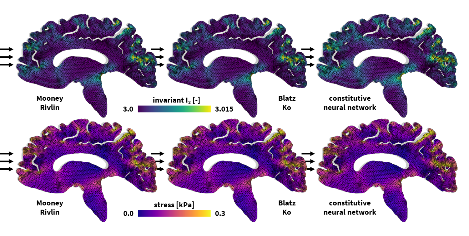
Figure 4: Universal material modeling of the human brain. Deformation and stress profiles for frontal impact to the human brain. The finite element models simulate the deformation and internal tissue loading corresponding to best-fit Mooney Rivlin, Blatz Ko, and newly discovered constitutive models from left to right. All simulations leverage our universal material model subroutine and only differ in the definition of the UNIVERSAL_TAB constitutive parameter table in the finite element analysis input file.

4 Applications

In the following sections, we showcase examples of soft matter systems where our universal material model subroutine naturally integrates mechanical testing from the material point level to the structural level.

4.1 The human brain

Brain tissue is among the softest and most vulnerable tissues in the human body [10]. The tissue’s delicate packing of neurons, glial cells, and extracellular matrix functionally regulates most vital processes in the human body and governs human cognition, learning, and consciousness [24]. As mechanics play a crucial role in neuronal function and dysfunction [32], understanding the mechanical behavior of brain tissue is essential for anticipating how the brain will respond to injury, how it evolves during its development, or how it remodels as disease advances. Computational models play a crucial role in this endeavor, allowing researchers to simulate the multi-faceted behavior of brain tissue and explore the biomechanical role of mechanical forces in health and disease [38, 57, 76, 110]. These models require adequate constitutive models that capture the complex and unique characteristics of this ultrasoft, highly adaptive, and heterogeneous tissue.

Constitutive modeling

Over the past decade, various research groups around the world have made significant process in the experimental and constitutive characterization of human brain tissue [8]. This has led to multiple competing constitutive models to characterize the behavior of gray and white matter tissue. Most notably, neo Hooke [104], Blatz Ko [7], Mooney Rivlin [71, 89], Demiray [18], Gent [30], and Holzapfel [40] models were proposed as successful candidates to characterize the stress-stretch response of these tissues. Given brain tissue’s intricate behavior, fitting a constitutive model to one single loading mode, tension, compression, or shear, does not generalize well to the other modes [61, 98]. Therefore, we consider a widely-used benchmark dataset where $5\times 5\times 5$mm³ human brain samples were tested in tension, compression, and shear [8, 9, 10]. We concomitantly discover and fit the best possible constitutive models considering these loading modes together and find the following three best models and parameters [61].
The Mooney Rivlin model [71, 89]

$$\psi=\frac{1}{2}\mu_{1}\left(\bar{I}_{1}-3\right)+\frac{1}{2}\mu_{2}\left(\bar{I}_{2}-3\right)$$

with parameters $\mu_{1}=0.0021$ kPa, $\mu_{2}=1.8817$ kPa for the gray matter cortex, and $\mu_{1}=0.0168$ kPa, $\mu_{2}=0.9697$ kPa for the white matter corona radiata. This translates into
$\begin{array}[]{@{}l}\mbox{{\bf{\tt{*PARAMETER TABLE, TYPE="UNIVERSAL\_TAB"}}}}\\ \begin{array}[]{ttttttt}1,&1,&1,&1,&1.0,&1.0,&\mu_{1}/2\\ 2,&1,&1,&1,&1.0,&1.0,&\mu_{2}/2\end{array}\end{array}$
The Blatz Ko model [7]

$$\psi=\frac{1}{2}\mu\left(\bar{I}_{2}-3\right)$$

with parameters $\mu=1.9043$ kPa for the gray matter cortex, and $\mu=0.9556$ kPa for the white matter corona radiata. This translates into
$\begin{array}[]{@{}l}\mbox{{\bf{\tt{*PARAMETER TABLE, TYPE="UNIVERSAL\_TAB"}}}}\\ \mbox{{\bf{\tt{2,1,1,1,1.0,1.0,$\mu$/2 }}}}\\ \end{array}$
Our newly discovered six-term model [61, 82]

$$\psi =\mu_{1}\left[\bar{I}_{2}-3\right]+\frac{a_{1}}{2b_{1}}\left[\exp\left(b_{1}\left[\bar{I}_{2}-3\right]\right)-1\right]$$

$$-\frac{\alpha_{1}}{2\beta_{1}}\ln\left(1-\beta_{1}\left[\bar{I}_{2}-3\right]\right)+\mu_{2}\left[\bar{I}_{2}-3\right]^{2}$$

$$+\frac{a_{2}}{2b_{2}}\left[\exp\left(b_{2}\left[\bar{I}_{2}-3\right]^{2}\right)-1\right]-\frac{\alpha_{2}}{2\beta_{2}}\ln\left(1-\beta_{2}\left[\bar{I}_{2}-3\right]^{2}\right)$$

with non-zero terms $\alpha_{1}=1.2520$ kPa, $\beta_{1}=0.9875$, $\mu_{2}=3.8007$ kPa, $a_{2}=6.2285$ kPa, $b_{2}=1.6495$, $\alpha_{2}=4.6743$ kPa, and $\beta_{2}=1.6663$ for the gray matter cortex and $\mu_{1}=0.2215$ kPa, $a_{1}=0.2350$ kPa, $b_{1}=0.2398$, $a_{2}=6.3703$ kPa, $b_{2}=1.8893$, $\alpha_{2}=4.5065$ kPa, and $\beta_{2}=1.1789$ for the white matter corona radiata. We translate this model into the following six-line parameter table of our universal material model:
$\begin{array}[]{@{}l}\mbox{{\bf{\tt{*PARAMETER TABLE, TYPE="UNIVERSAL\_TAB"}}}}\\ \begin{array}[]{ttttttt}2,&1,&1,&1,&1.0,&1.0,&\mu_{1}\\ 2,&1,&1,&2,&1.0,&b_{1},&a_{1}/2b_{1}\\ 2,&1,&1,&3,&1.0,&\beta_{1},&\alpha_{1}/2\beta_{1}\\ 2,&1,&2,&1,&1.0,&1.0,&\mu_{2}\\ 2,&1,&2,&2,&1.0,&b_{2},&a_{2}/2b_{2}\\ 2,&1,&2,&3,&1.0,&\beta_{2},&\alpha_{2}/2\beta_{2}\\ \end{array}\end{array}$

Simulation

Utilizing our universal material model subroutine, we incorporate these brain models into a realistic vertical head impact finite element simulation [82]. Based on magnetic resonance images [36], we create the two-dimensional sagittal finite element model in Figure 4. In this model, gray and white matter are spatially discretized using 6,182 gray and 5,701 white linear triangular elements, resulting in 6,441 nodes, and 12,882 degrees of freedom in total. We embed our model into the skull using spring support at the free boundaries and apply a frontal impact to the brain that we represent with all three models, the Mooney Rivlin, Blatz Ko, and new discovered models, as shown in Figure 4.

4.2 Skin

Skin is the largest organ of the human body [11]. It serves vital functions for our survival such as being the first line of defense against mechanical injury while at the same time allowing us to move and interact with the world [58]. Surgery of any kind entails skin rupture and manipulation [1]. Especially during reconstructive procedures, skin tissues are subjected to extreme deformations [56]. The complex stress field generated by skin tissue manipulation has a direct effect on the subsequent wound healing response, with excessive stress causing increased inflammatory response that can lead to fibrosis [55]. In some cases, excessive stress can even result in tissue necrosis [33]. Thus, accurate computational models of skin are key to design safe reconstructive surgical procedures.

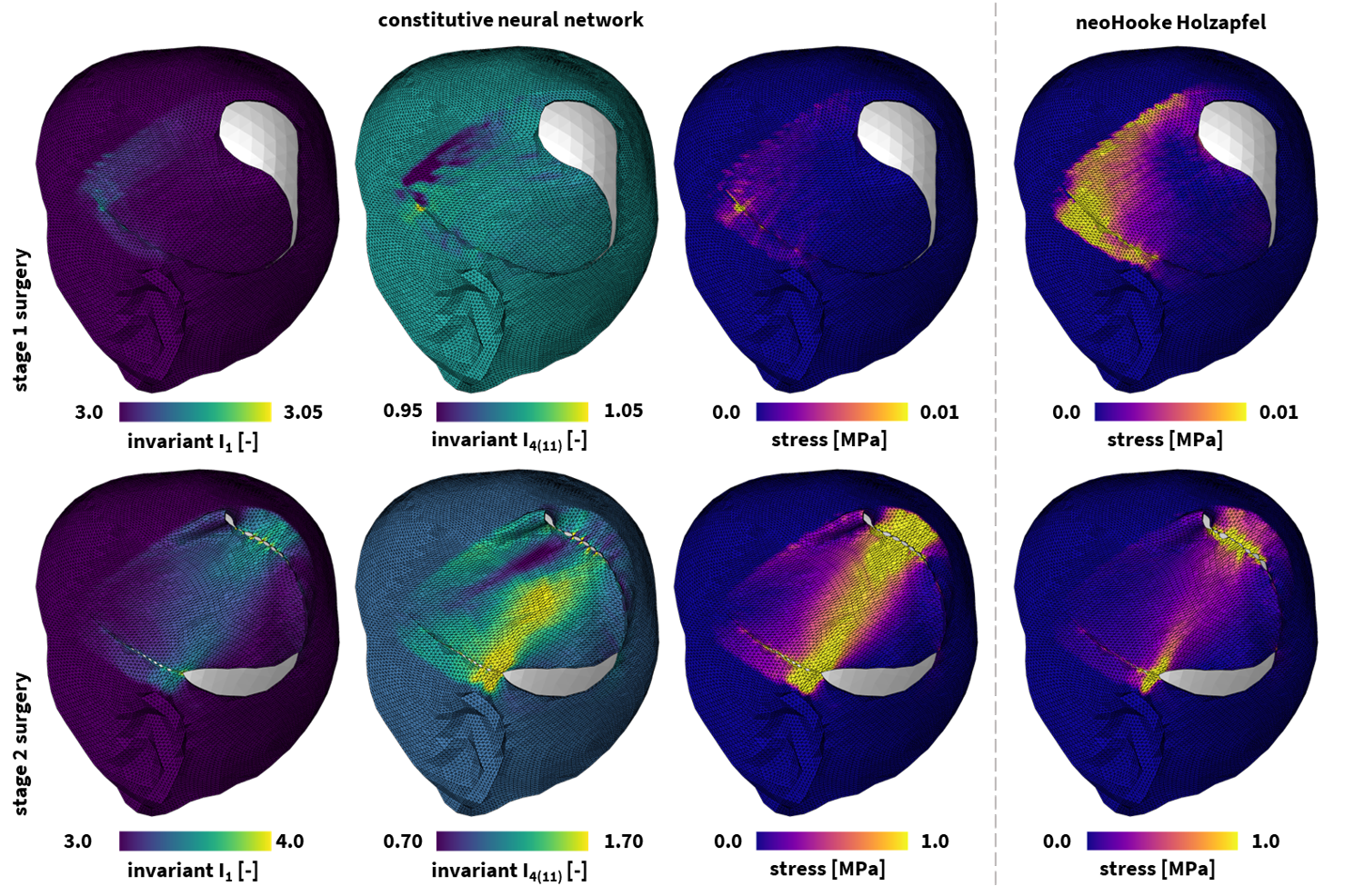
Figure 5: Universal material modeling of skin. Deformation and stress profiles in the human scalp following a melanoma resection reconstruction procedure. The finite element models simulate the deformation and internal tissue loading corresponding a two-stage flap rotation and suturing procedure, with the first stage shown in the top row and the second stage shown in the bottom row. The remaining wound is closed with a skin graft to avoid excessive tissue stresses and damage. Both tissue manipulations are modeled using the best-fit constitutive neural network model in the three left columns. For comparison, we also showcase the resulting stress profiles for the best-fit neo Hooke Holzapfel model in the right column. All simulations leverage our universal material model subroutine and only differ in the definition of the UNIVERSAL_TAB constitutive parameter table in the finite element analysis input file.

Constitutive modeling

Skin modeling has received significant attention for more than half a century [53, 103]. Isotropic models such as the neo Hooke [104] or Mooney Rivlin [71, 89] models have been used, but show significant limitations. Not only do they fail to describe the anisotropy of skin, they also lack the ability to capture this tissue’s rapid strain-stiffening behavior [53]. To overcome these issues, we examine combined uniaxial and biaxial tensile testing data of porcine skin tissue samples [99, 100] to discover more accurate material models that depict the anisotropic stress-stretch behavior. First, we fit the microstructure-inspired Holzapfel model [40],

$$\psi=\frac{1}{2}\mu\left[\bar{I}_{1}-3\right]+\frac{1}{2}\frac{a_{4}}{b_{4}}\left[\exp\left(b_{4}\langle\bar{I}_{4(11)}-1\rangle^{2}\right)-1\right]\,.$$

This model was originally developed for arterial tissues and combines the isotropic linear first invariant neo Hooke term, $\left[\bar{I}_{1}-3\right]$, with an anisotropic quadratic exponential fourth invariant term, $\langle\bar{I}_{4(11)}-1\rangle$, along the collagen fiber direction. Here, our best possible fit to the combined uniaxial and biaxial testing data results in $\mu=0.2492$ MPa, $a_{4}=0.1054$ MPa, and $b_{4}=10.7914$. We naturally incorporate this constitutive model and parameters in our universal material model subroutine using the following two-line parameter table
$\begin{array}[]{@{}l}\mbox{{\bf{\tt{*PARAMETER TABLE, TYPE="UNIVERSAL\_TAB"}}}}\\ \begin{array}[]{ttttttt}1,&1,&1,&1,&1.0,&1.0,&\mu\\ 4,&2,&2,&2,&1.0,&b_{4},&a_{4}/2b_{4}\end{array}\end{array}$
Given the rather low mean goodness of fit $\rm{R}^{2}=0.6857$, we subsequently leverage a tranversely isotropic constitutitive neural network to discover a more accurate model [59]. From a library of $2^{16}=65,536$ possible combinations of terms, we discover a model in two exponential quadratic terms,

$$\psi =\frac{a_{1}}{2b_{1}}\left(\exp{\left[b_{1}\left(\bar{I}_{1}-3\right)^{2}\right]}-1\right)$$

$$+\frac{a_{4}}{2b_{4}}\left(\exp{\left[b_{4}\langle\bar{I}_{4(11)}-1\rangle^{2}\right]}-1\right)$$

with parameters $a_{1}=1.3291$ MPa, $b_{1}=0.8207$, $a_{4}=0.2656$ MPa, and $b_{4}=0.3921$ [59]. To integrate this new model into a finite element simulation, we incorporate the following two parameter lines in our universal material subroutine
$\begin{array}[]{@{}l}\mbox{{\bf{\tt{*PARAMETER TABLE, TYPE="UNIVERSAL\_TAB"}}}}\\ \begin{array}[]{ttttttt}1,&1,&2,&2,&1.0,&b_{1},&a_{1}/2b_{1}\\ 4,&2,&2,&2,&1.0,&b_{4},&a_{4}/2b_{4}\end{array}\end{array}$
In contrast to the neo Hooke Holzapfel model, this discovered constitutive neural network model has a mean good of fit $\rm{R}^{2}=0.8629$ for the combined uniaxial and biaxial porcine skin testing data [59].

Simulation

Leveraging our universal material subroutine, we integrate both material models in a finite element simulation of a 62-year-old adult male patient undergoing reconstructive surgery following surgical melanoma resection [56]. A three-dimensional patient specific geometry was obtained via multi-view stereo reconstruction of a sequence of photos taken in the operating room before and after surgery. The scalp was approximated based on the skin surface and spatially discretized using 75,282 linear tetrahedral elements and 25,394 nodes, leading to a total 76,182 degrees of freedom. Our simulation recapitulates the closure of the resected tissue defect by imposing nodal constraints to nodes on either edge of the defect to mimic sutures used to close the wound. Figure 5 showcases the deformation and internal tissue tension profiles following the two-step surgical skin reconstruction procedure. We clearly observe the limited tissue deformation and loading profiles during the first stage in the top row. In contrast, during the second stage surgery in the bottom row, substantial deformations develop across the skin. Specifically, we appreciate the regional differences between the isotropic $\bar{I}_{1}$ and anisotropic $\bar{I}_{4(11)}$ deformation invariants. Figure 5 also showcases noticeable stress profile differences between the newly discovered material model and the neo Hooke Holzapfel model in the third and fourth columns. In the lower stretch regimes shown in the first stage reconstruction, the neo Hooke Holzapfel model clearly overestimates the stresses in the skin. In the higher stretch regimes, shown during the second stage reconstruction in the bottom, the neo Hooke Holzapfel fit underestimates the stresses in the tissue. While a modeling-based overestimation of the stress state holds limited risks from a medical point of view, an underestimation could have harmful consequences as clinical decisions co-informed by such models could cause excessive tissue damage and scarring. Figure 5 showcases the crucial aspect that proper constitutive modeling and calibration plays in this regard, in which the neo Hooke Holzapfel model, which does not properly capture skin tissue’s strain-stiffening, underestimates the tissue stress in comparison to the more accurate newly discovered model.

4.3 Human arteries

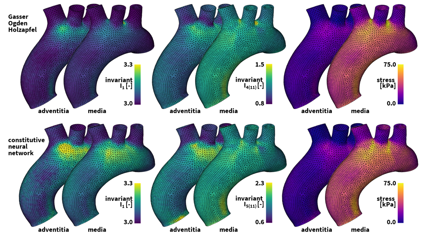
Figure 6: Universal material modeling of human arteries. Diastolic deformation and stress profiles in the media and adventitia layer of the human ascending aortic arch. The finite element models simulate the deformation and internal tissue loading corresponding to the best-fit Holzapfel dispersion model in the top row and newly discovered model in the bottom row. Both simulations leverage our universal material model subroutine and only differ in the definition of the UNIVERSAL_TAB constitutive parameter table in the finite element analysis input file.

Computational simulations play a pivotal role in understanding and predicting the biomechanical factors of a wide variety of arterial diseases [44, 79, 105]. In vascular medicine, knowing the precise stress and strain fields across the vascular wall is critical for understanding the formation, growth, and rupture of aneurysms and dissections [45, 108, 31]; for identifying high-risk regions of plaque formation, rupture, and thrombosis [43, 87]; and for optimizing stent design and surgery [16, 21].

Constitutive modeling

Over the past four decades, various phenomenological polynomial [107, 109], exponential [27], logarithmic [101], and exponential-polynomial [49, 81, 114] models have been proposed to describe the non-linear elastic, anisotropic, quasi-incompressible behavior of arterial tissue. Recently, microstructurally-informed models were brought forward, including symmetric two- and four-fiber family models [28, 40, 6], either symmetric or unsymmetric [41]. All these material models can fit uniaxial and biaxial arterial tissue testing data, but do not always generalize well to off-axis testing regimes [93].
We consider biaxial tensile testing of thoracic aortic tissue samples at five differing circumferential-axial stretch ratios [74, 73] Using data-driven constitutive neural networks, we discover the most appropriate arterial material model. From a library of $2^{16}=65,536$ possible combinations of terms, we discover

$$\psi =\frac{\mu_{1}}{2}\left[\bar{I}_{1}-3\right]+\frac{a}{2b}\left(\exp{\left[b\left(\bar{I}_{1}-3\right)\right]}-1\right)$$

$$+\sum_{i=1,2}\frac{1}{2}\mu_{5}\left\langle\bar{I}_{5(ii)}-1\right\rangle^{2}$$

with an isotropic linear and exponential linear first invariant term and an anisotropic quadratic fifth invariant term. Our best-fit parameters read $\mu_{1}=33.45$ kPa, $a=3.74$ kPa, $b=6.66$, $\mu_{5}=2.17$ kPa for the media at an angle $\alpha=\pm 7.00^{\circ}$ and $\mu_{1}=8.30$ kPa, $a=1.42$ kPa, $b=6.34$, $\mu_{5}=0.49$ kPa for the adventitia at an angle $\alpha=\pm 66.78^{\circ}$. This translates into the following four-line parameter table of our universal material model,
$\begin{array}[]{@{}l}\mbox{{\bf{\tt{*PARAMETER TABLE, TYPE="UNIVERSAL\_TAB"}}}}\\ \begin{array}[]{ttttttt}1,&1,&1,&1,&1.0,&1.0,&\mu_{1}/2\\ 1,&1,&1,&2,&1.0,&b,&a/2b\\ 5,&2,&2,&1,&1.0,&1.0,&\mu_{5}/2\\ 9,&2,&2,&1,&1.0,&1.0,&\mu_{5}/2\\ \end{array}\end{array}$
Alternatively, in the classical microstructure-inspired dispersion type Holzapfel model [43]

$$\psi=\frac{1}{2}\mu\left[\bar{I}_{1}-3\right]+\sum_{i=1,2}\frac{a}{2b}\left(\exp{\left[b\langle\bar{I}_{1/4(ii)}^{*}-1\rangle^{2}\right]}-1\right)$$

our best-fit parameters are $\mu=48.68$ kPa, $a=6.67$ kPa, $b=23.17$, $\kappa=0.074$ for the media at $\alpha=\pm 7.00^{\circ}$) and $\mu=13.22$ kPa, $a=0.93$ kPa, $b=12.06$, $\kappa=0.091$ for the adventitia at $\alpha=\pm 66.78^{\circ}$. We translate this model into the following parameter table of our universal material model
$\begin{array}[]{@{}l}\mbox{{\bf{\tt{*PARAMETER TABLE, TYPE="MIXED\_INV"}}}}\\ \mbox{{\bf{\tt{1,$\kappa$,0.0,0.0,$(1-3\kappa)$,0.0,0.0,0.0,0.0,0.0,}}}}\\ \hskip 8.5359pt\mbox{{\bf{\tt{0.0,0.0,0.0,0.0,0.0,0.0}}}}\\ \mbox{{\bf{\tt{1,$\kappa$,0.0,0.0,0.0,0.0,0.0,0.0,$(1-3\kappa)$,0.0,}}}}\\ \hskip 8.5359pt\mbox{{\bf{\tt{0.0,0.0,0.0,0.0,0.0,0.0}}}}\\ \mbox{{\bf{\tt{*PARAMETER TABLE, TYPE="UNIVERSAL\_TAB"}}}}\\ \begin{array}[]{ttttttt}1,&1,&1,&1,&1.0,&1.0,&\mu/2\\ 101,&2,&2,&2,&1.0,&b,&a/2b\\ 102,&2,&2,&2,&1.0,&b,&a/2b\end{array}\end{array}$

Simulation

Using our universal material subroutine, we integrate both models in a finite element simulation of the human aortic arch under hemodynamic loading conditions [80]. Our aortic arch geometry is extracted from high-resolution magnetic resonance images of a healthy, 50th percentile U.S. male [78]. We assume an average aortic wall thickness of 3.0 mm, where the inner 75% of the wall make up the media and the outer 25% make up the adventitia. We discretize our geometry using 60,684 linear tetrahedral elements for the media and 30,342 linear tetrahedral elements for the adventitia, leading to a total 61,692 degrees of freedom. The local collagen fiber angles against the circumferential direction are $\pm$ 7.00^∘ in the media and $\pm$ 66.78^∘ in the adventitia and are locally defined as a vector field variable for each element. We use continuum distributed coupling boundary conditions at the aortic outlets to constrain the arch in space [83], and leverage Neumann boundary conditions to simulate the hemodynamic loading conditions the aortic arch undergoes during a single cardiac cycle. Figure 6 showcases the computed diastolic stresses in the media and the adventitia for both our newly discovered model and the microstructure-informed dispersion-type Holzapfel model [81].

4.4 Heart valves

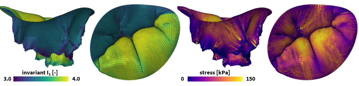
Figure 7: Universal material modeling of heart valves. Personalized tricuspid valve loading during the cardiac cycle. The finite element models simulate the deformation, left, and internal tissue loading, right, in response to the inter-ventricular pressure changes from end-diastole to end-systole. The tricuspid valve is shown from a side and top view. Each valvular leaflet leverages our universal material model subroutine and only differs in the definition of the UNIVERSAL_TAB constitutive parameter table in the finite element analysis input file.

The tricuspid valve is our right atrioventricular valve which ensures unidirectional blood flow through the right side of the heart. Often as a result of other primary diseases [90, 20], a diseased tricuspid valve can fail to close and regurgitate. Tricuspid valve disease affects over one million Americans and is associated with increased patient mortality and morbidity [72, 75]. Computational models of the tricuspid valve provide valuable insights into the workings of the valve, and have been used to increase our understanding of the progression of valve disease [65] and to work towards improved repair outcomes [35].

Constitutive modeling

Numerous studies have investigated the mechanical behavior of atrioventricular valve leaflets. Valvular leaflets exhibit a pronounced anisotropy and a non-linear behavior, motivating an anisotropic exponential material model to capture this complex material behavior [54]. Others have used microstructurally-informed models [28, 52] or anisotropic exponential Fung-type models [50] to capture the material response of the tricuspid valve leaflets. However, the tricuspid valve leaflets only exhibit slight anisotropy [84]. To improve the ease of use in computational models, recent studies have proposed a simplified isotropic Fung-type exponential function [48]. Leveraging force-controlled 400 mN equibiaxial mechanical tests on 7$\times$7 mm valve leaflet tissue samples [67], we fit the following two-term isotropic exponential Fung-Type model [66]

$$\psi=\,\frac{c_{0}}{2}\left[\bar{I}_{1}-3\right]+\frac{c_{1}}{2}\left(\exp{\left[c_{2}\left(\bar{I}_{1}-3\right)^{2}\right]}-1\right)$$

with an isotropic linear first invariant term describing the response at small-strains and under compression and an exponential first invariant term determining the strain-stiffening response under large strains [48]. Our best-fit parameters are $c_{0}=1.0$ kPa, $c_{1}=0.124$ kPa, $c_{2}=4.57$ for the anterior, $c_{0}=1.0$ kPa, $c_{1}=0.188$ kPa, $c_{2}=14.86$ for the posterior, and $c_{0}=1.0$ kPa, $c_{1}=0.191$ kPa, $c_{2}=17.75$ for the septal leaflets. To incorporate this constitutive model in our universal material subroutine, we define the following two parameter lines
$\begin{array}[]{@{}l}\mbox{{\bf{\tt{*PARAMETER TABLE, TYPE="UNIVERSAL\_TAB"}}}}\\ \begin{array}[]{ttttttt}1,&1,&1,&1,&1.0,&1.0,&c_{0}/2\\ 1,&1,&2,&2,&1.0,&c_{2},&c_{1}/2\end{array}\end{array}$

Simulation

Using our universal material subroutine, we integrate the constitutive behavior of all three leaflets into a personalized finite element model of the tricuspid valve, the Texas 1.1 TriValve [66, 106]. Through personalized pressure and annular displacement recordings in the realistic hemodynamic environment of an organ preservation system and image-based planimetry on the excised valve, a three-dimensional reconstruction of the tricuspid valve is build at end-diastole. The valve and chordae geometries are spatially discretized using 8,283 linear quadrilaterial shell elements and 4,169 three-dimensional linear multi-segmented truss elements, resulting in a total 25,761 degrees of freedom. By imposing the recorded personalized annular displacements and an end-systolic transvalvular pressure of 22.95 mmHg on the ventricular surface of the valve, we simulate valvular loading from end-diastole to end-systole. Figure 7 showcases the resulting deformation and maximum principal stress contours the tricuspid valve. Notably, the varying stiffnesses of the anterior, septal, and posterior leaflets result in noticeable differences in the first invariant of the Cauchy-Green deformation tensor, but in comparable maximum principal stress profiles across the leaflets.

4.5 The human heart

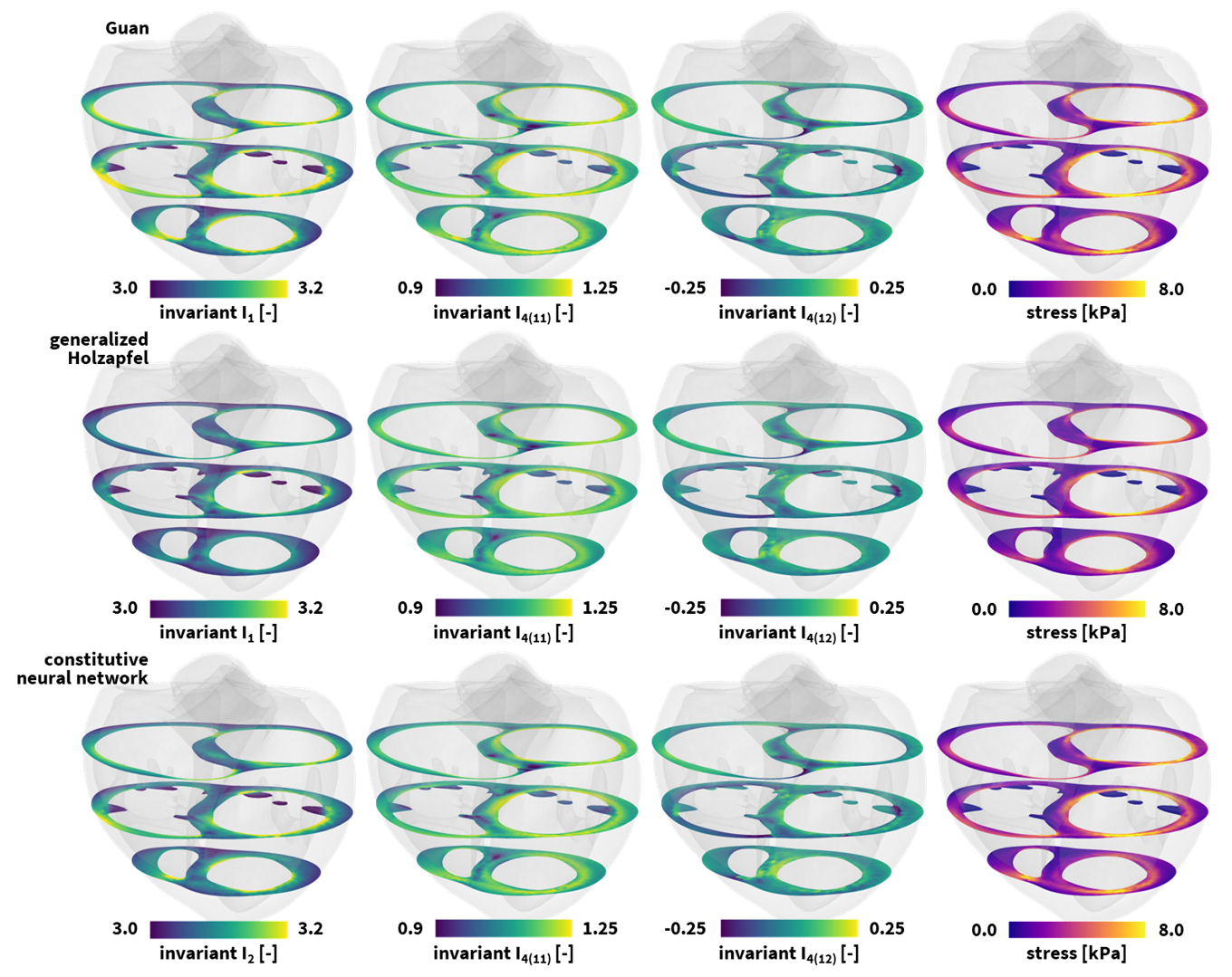
Figure 8: Universal material modeling of the human heart. Personalized isotropic and directional deformation invariant and maximum principal stresses stress profiles, in short-axis slices frontal views, resulting from a healthy left and right ventricular end-diastolic pressure loading of 8mmHg and 4mmHg. The finite element models simulate the deformation and internal tissue loading corresponding to the best-fit Guan model in the top row, the generalized Holzapfel model in the middle row, and the newly discovered model in the bottom row. All three simulations leverage our universal material model subroutine and only differ in the definition of the UNIVERSAL_TAB constitutive parameter table in the finite element analysis input file.

Cardiac disorders are a leading cause of morbidity and death worldwide [68]. Computational models of cardiac function hold immense potential to contribute to our understanding of health and disease, improve our diagnostic analyses, and optimize personalized intervention [78, 5, 22]. For example, corrective surgeries in obstructive cardiomyopathy [86] and congenital heart defects [102], the replacement of diseased valves [26], or the implantation of a cardiac assist device [91] all involve complex and delicate procedures that demand careful planning and simulation to ensure their success. Crucially, the accuracy and reliability of these computational models hinge on precise constitutive modeling of the underlying mechanical behavior of myocardial tissue.

Constitutive modeling

Research on constitutive models that accurately describe passive myocardial mechanics spans over five decades. One of the earliest models described cardiac muscle tissue as an isotropic hyperelastic material [17]. Later, with increasing experimental insights, more sophisticated transversely isotropic [46, 14], and eventually orthotropic [92, 42] constitutive models were introduced. This latter cardiac-tissue Holzapfel model is currently one of the most popular models for heart muscle tissue and fits simple shear tests of myocardial tissue well [19]. Nevertheless, it displays limitations when simultaneously fitted to different loading modes [34]. Therefore, we consider triaxial shear and biaxial extension tests on human myocardial tissue [95], and use these data to discover and the best possible model and parameters to characterize both loading conditions combined [64].
We begin with the four-term Guan model [34] that features an exponential linear term in the first invariant $\bar{I}_{1}$, exponential quadratic terms in the fiber and normal fourth invariants $\bar{I}_{\rm{4f}}$ and $\bar{I}_{\rm{4n}}$, and an exponential quadratic term in the fiber-sheet eighth invariant $\bar{I}_{\rm{8fs}}$,

$$\psi =\frac{a}{2b}\left[\,\exp\left(b[\bar{I}_{1}-3]\right)\right]+\frac{a_{\rm{f}}}{2b_{\rm{f}}}\,\left[\,\exp\left(b_{\rm{f}}\langle\bar{I}_{\rm{4f}}-1\rangle^{2}\right)-1\right]$$

$$+\frac{a_{\rm{n}}}{2b_{\rm{n}}}\,[\,\exp\left(b_{\rm{n}}\langle\bar{I}_{\rm{4n}}-1\rangle^{2}\right)-1]+\frac{a_{\rm{fs}}}{2b_{\rm{fs}}}[\,\exp\left(b_{\rm{fs}}[I_{\rm{8fs}}]^{2}\right)-1].$$

Calibrating this model simultaneously on biaxial tensile and triaxial shear data for human myocardial tissue, we obtain a mean goodness of fit $\rm{R}^{2}=0.867$ for parameters $a=0.782$ kPa, $b=7.248$, $a_{\rm{f}}=4.488$ kPa, $b_{\rm{f}}=14.571$, $a_{\rm{n}}=2.513$ kPa, $b_{\rm{n}}=10.929$, $a_{\rm{fs}}=0.436$ kPa, and $b_{\rm{fs}}=4.959$. To incorporate this constitutive model in our universal material subroutine, we define the following four parameter lines,

$\begin{array}[]{@{}l}\mbox{{\bf{\tt{*PARAMETER TABLE, TYPE="UNIVERSAL\_TAB"}}}}\\ \begin{array}[]{ttttttt}1,&1,&1,&2,&1.0,&b,&a/2b\\ 4,&2,&2,&2,&1.0,&b_{f},&a_{f}/2b_{f}\\ 14,&2,&2,&2,&1.0,&b_{n},&a_{n}/2b_{n}\\ 6,&1,&2,&2,&1.0,&b_{fs},&a_{fs}/2b_{fs}\end{array}\end{array}$

Next, we consider the seven-term generalized Holzapfel model [42] which features an exponential linear term in the first invariant $\bar{I}_{1}$, exponential quadratic terms of all fourth invariants $\bar{I}_{\rm{4f}}$, $\bar{I}_{\rm{4s}}$, $\bar{I}_{\rm{4n}}$, and an exponential quadratic term in all eighth invariants $\bar{I}_{\rm{8fs}}$, $\bar{I}_{\rm{8fn}}$, $\bar{I}_{\rm{8sn}}$.

$$\psi =\frac{a}{2b}\left[\,\exp\left(b[\bar{I}_{1}-3]\right)\right]+\frac{a_{\rm{f}}}{2b_{\rm{f}}}\,\left[\,\exp\left(b_{\rm{f}}\langle\bar{I}_{\rm{4f}}-1\rangle^{2}\right)-1\right]$$

$$+\frac{a_{\rm{s}}}{2b_{\rm{s}}}\,[\,\exp\left(b_{\rm{s}}\langle\bar{I}_{\rm{4s}}-1\rangle^{2}\right)-1]+\frac{a_{\rm{n}}}{2b_{\rm{n}}}\,[\,\exp\left(b_{\rm{n}}\langle\bar{I}_{\rm{4n}}-1\rangle^{2}\right)-1]$$

$$+\frac{a_{\rm{fs}}}{2b_{\rm{fs}}}[\,\exp\left(b_{\rm{fs}}[\bar{I}_{\rm{8fs}}]^{2}\right)-1]+\frac{a_{\rm{sn}}}{2b_{\rm{sn}}}[\,\exp\left(b_{\rm{sn}}[\bar{I}_{\rm{8sn}}]^{2}\right)-1].$$

A combined triaxial-biaxial training of this model calibrates the model parameters to $a=0.950$ kPa, $b=5.457$, $a_{\rm{f}}=3.318$ kPa, $b_{\rm{f}}=23.701$, $a_{\rm{s}}=1.405$ kPa, $b_{\rm{s}}=20.067$, $a_{\rm{n}}=2.037$ kPa, $b_{\rm{n}}=16.976$, $a_{\rm{fs}}=0.586$ kPa, $b_{\rm{fs}}=1.081$, $a_{\rm{sn}}=0.047$ kPa, and $b_{\rm{sn}}=11.842$. This model has a mean goodness of fit $\rm{R}^{2}=0.876$ [64]. We translate this constitutive model into our universal material subroutine through the definition of the following parameter lines in our finite element analysis input file

$\begin{array}[]{@{}l}\mbox{{\bf{\tt{*PARAMETER TABLE, TYPE="UNIVERSAL\_TAB"}}}}\\ \begin{array}[]{ttttttt}1,&1,&1,&2,&1.0,&b,&a/2b\\ 4,&2,&2,&2,&1.0,&b_{f},&a_{f}/2b_{f}\\ 8,&2,&2,&2,&1.0,&b_{s},&a_{s}/2b_{s}\\ 14,&2,&2,&2,&1.0,&b_{n},&a_{n}/2b_{n}\\ 6,&1,&2,&2,&1.0,&b_{fs},&a_{fs}/2b_{fs}\\ 12,&1,&2,&2,&1.0,&b_{sn},&a_{sn}/2b_{sn}\\ \end{array}\end{array}$

Finally, we leverage an orthotropic constitutive neural network to discover the best model and parameters to explain the experimental data. From a library of $2^{32}=4,294,967,296$ possible combinations of terms and a sparsity-promoting regularization with $\alpha=0.01$, we discover a four-term model,

$$\psi =\mu\left(\bar{I}_{2}-3\right)^{2}+\frac{a_{\rm{f}}}{2b_{\rm{f}}}\,\left[\,\exp\left(b_{\rm{f}}\langle\bar{I}_{\rm{4f}}-1\rangle^{2}\right)-1\right]$$

$$+\frac{a_{\rm{n}}}{2b_{\rm{n}}}\,[\,\exp\left(b_{\rm{n}}\langle\bar{I}_{\rm{4n}}-1\rangle^{2}\right)-1]+\frac{a_{\rm{fs}}}{2b_{\rm{fs}}}[\,\exp\left(b_{\rm{fs}}[\bar{I}_{\rm{8fs}}]^{2}\right)-1].$$

with a mean goodness of fit $\rm{R}^{2}=0.894$ [64]. Here, our discovered material parameters amount to $\mu=5.162$ kPa, $a_{\rm{f}}=3.426$ kPa, $b_{\rm{f}}=21.151$, $a_{\rm{n}}=2.754$ kPa, $b_{\rm{n}}=4.371$, $a_{\rm{fs}}=0.494$ kPa, and $b_{\rm{fs}}=0.508$. We integrate this newly discovered model for myocardial tissue in our finite element analysis through the following four-line parameter table

$\begin{array}[]{@{}l}\mbox{{\bf{\tt{*PARAMETER TABLE, TYPE="UNIVERSAL\_TAB"}}}}\\ \begin{array}[]{ttttttt}2,&1,&1,&2,&1.0,&1.0,&\mu/2\\ 4,&2,&2,&2,&1.0,&b_{f},&a_{f}/2b_{f}\\ 14,&2,&2,&2,&1.0,&b_{n},&a_{n}/2b_{n}\\ 6,&1,&2,&2,&1.0,&b_{fs},&a_{fs}/2b_{fs}\end{array}\end{array}$

Simulation

We incorporate all three constitutive models for myocardial tissue in the finite element analysis software solver Abaqus [15] using our universal material subroutine, and predict the stress state of the left and right ventricular wall during diastolic filling. We create a finite element model of the left and right ventricular myocardial wall from high-resolution magnetic resonance images of a healthy 44-year-old Caucasian male with a height of 178 cm and weight of 70 kg [80, 78]. We spatially discretize our computational domain using 99,286 quadratic tetrahedral elements and 154,166 nodes, leading to a total 462,498 degrees of freedom. We compute the helically wrapped myofibers by solving a Laplace-Dirichlet problem across our computational domain, and assume a transmural fiber variation from +60^∘ to -60 ^∘ from the endocardial to the epicardial wall [111]. The resulting microstructural organization covers 99,286 local element-based fiber, sheet, and normal vectors, $\bm{f}_{0}$, $\bm{s}_{0}$, $\bm{n}_{0}$. We apply homogeneous Dirichlet boundary conditions at the mitral, aortic, tricupid, and pulmonary valve annuli to fix the heart in space [83], and load it with hemodynamic Neumann boundary conditions that correspond to the endocardial blood pressure during diastolic filling. Figure 8 showcases the resulting deformation and stress profiles in both ventricles in response to left and right ventricular pressures of 8 mmHg and 4 mmHg. In a row-to-row comparison of the short-axis views, we observe small differences between the deformation invariants and the maximum principal wall stresses of all three models, with larger values for our newly discovered model and the Guan model and smaller values for the generalized myocardial Holzapfel model. We can explain these differences by the differing goodness of fit of the three models. Moreover, we observe that our diastolic hemodynamic loading conditions enforce deformation and stress states that surpass the homogeneous tissue testing protocols of the triaxial shear and biaxial extension training data, which creates local regions of extrapolation beyond the initial training regime [64]. Taken together, while our discovered four-parameter model best explains the laboratory experiments of triaxial shear and biaxial extension, all three models translate well into a single universal material subroutine and predict fairly similar stress profiles across the human heart.

5 Conclusion

In this work, we designed a universal constitutive modeling framework to predict the mechanical behavior of soft materials across a wide range of applications. We set up a modular material subroutine architecture which seamlessly integrates with Abaqus, and can easily be generalized towards other non-linear finite element analysis solvers. Doing so, our framework mitigates the risk for human error and streamlines the integration of newly discovered material models in their simulations, thus alleviating the users to perform lengthy algebraic derivations and extensive programming. Furthermore, our material subroutine serves as an excellent verification tool for more expert finite element software developers aiming to debug their own soft material models and finite element analysis implementations. We demonstrated the versatility of the universal material subroutine through numerical simulations of various living systems including the brain, skins, arteries, valves and the human heart. Providing a common language and material subroutine for the computational mechanics community at large, we aspire to democratize the computational analysis of soft materials amongst a broader cohort of researchers and engineers. With one single subroutine, everyone - and not just a small group of expert specialists - can now perform reliable engineering analysis of artificial organs, stretchable electronics, soft robotics, smart textiles, and even artificial meat. Fostering this inclusivity, our framework can form an invaluable tool towards continued innovation and discovery in the field of soft matter overall.

References

- [1] Shahram Aarabi, Michael T Longaker, and Geoffrey C Gurtner. Hypertrophic scar formation following burns and trauma: new approaches to treatment. PLoS Medicine, 4(9):e234, September 2007.
- [2] Pasquale Claudio Africa. life: A flexible, high performance library for the numerical solution of complex finite element problems. SoftwareX, 20:101252, December 2022.
- [3] Garth Wells Anders Logg, Kent-Andre Mardal, editor. Automated solution of differential equations by the finite element method: the FEniCS book. Springer Berlin Heidelberg, 2012.
- [4] Stuart S. Antman. Nonlinear problems of elasticity. Springer-Verlag, 2005.
- [5] Christoph M. Augustin, Matthias A.F. Gsell, Elias Karabelas, Erik Willemen, Frits W. Prinzen, Joost Lumens, Edward J. Vigmond, and Gernot Plank. A computationally efficient physiologically comprehensive 3D–0D closed-loop model of the heart and circulation. Computer Methods in Applied Mechanics and Engineering, 386:114092, December 2021.
- [6] S. Baek, R.L. Gleason, K.R. Rajagopal, and J.D. Humphrey. Theory of small on large: potential utility in computations of fluid-solid interactions in arteries. Computer Methods in Applied Mechanics and Engineering, 196(31–32):3070–3078, June 2007.
- [7] Paul J. Blatz and William L. Ko. Application of finite elastic theory to the deformation of rubbery materials. Transactions of the Society of Rheology, 6(1):223–252, March 1962.
- [8] S. Budday, G. Sommer, C. Birkl, C. Langkammer, J. Haybaeck, J. Kohnert, M. Bauer, F. Paulsen, P. Steinmann, E. Kuhl, and G.A. Holzapfel. Mechanical characterization of human brain tissue. Acta Biomaterialia, 48:319–340, January 2017.
- [9] S. Budday, G. Sommer, J. Haybaeck, P. Steinmann, G.A. Holzapfel, and E. Kuhl. Rheological characterization of human brain tissue. Acta Biomaterialia, 60:315–329, September 2017.
- [10] Silvia Budday, Timothy C. Ovaert, Gerhard A. Holzapfel, Paul Steinmann, and Ellen Kuhl. Fifty shades of brain: a review on the mechanical testing and modeling of brain tissue. Archives of Computational Methods in Engineering, 27(4):1187–1230, July 2019.
- [11] Adrián Buganza Tepole, Christopher Joseph Ploch, Jonathan Wong, Arun K. Gosain, and Ellen Kuhl. Growing skin: A computational model for skin expansion in reconstructive surgery. Journal of the Mechanics and Physics of Solids, 59(10):2177–2190, October 2011.
- [12] Bernard D Coleman and Walter Noll. On the thermostatics of continuous media. Archive for rational mechanics and analysis, 4:97–128, 1959.
- [13] Stephen John Connolly, Donald Mackenzie, and Yevgen Gorash. Higher-order and higher floating-point precision numerical approximations of finite strain elasticity moduli. International Journal for Numerical Methods in Engineering, 120(10):1184–1201, August 2019.
- [14] K. D. Costa, P. J. Hunter, J. S. Wayne, L. K. Waldman, J. M. Guccione, and A. D. McCulloch. A three-dimensional finite element method for large elastic deformations of ventricular myocardium: ii—prolate spheroidal coordinates. Journal of Biomechanical Engineering, 118(4):464–472, November 1996.
- [15] Dassault Systèmes Simulia Corp. Abaqus Analysis User’s Guide. Rhode Island, 2024.
- [16] S. De Bock, F. Iannaccone, G. De Santis, M. De Beule, D. Van Loo, D. Devos, F. Vermassen, P. Segers, and B. Verhegghe. Virtual evaluation of stent graft deployment: a validated modeling and simulation study. Journal of the Mechanical Behavior of Biomedical Materials, 13:129–139, September 2012.
- [17] H. Demiray. Stresses in ventricular wall. Journal of Applied Mechanics, 43(2):194–197, June 1976.
- [18] Hilmi Demiray. A note on the elasticity of soft biological tissues. Journal of Biomechanics, 5(3):309–311, May 1972.
- [19] Socrates Dokos, Bruce H. Smaill, Alistair A. Young, and Ian J. LeGrice. Shear properties of passive ventricular myocardium. American Journal of Physiology-Heart and Circulatory Physiology, 283(6):H2650–H2659, December 2002.
- [20] Gilles D. Dreyfus, Randolph P. Martin, K.M. John Chan, Filip Dulguerov, and Clara Alexandrescu. Functional tricuspid regurgitation. Journal of the American College of Cardiology, 65(21):2331–2336, June 2015.
- [21] Nele Famaey, Gerhard Sommer, Jos Vander Sloten, and Gerhard A. Holzapfel. Arterial clamping: finite element simulation and in vivo validation. Journal of the Mechanical Behavior of Biomedical Materials, 12:107–118, August 2012.
- [22] Marco Fedele, Roberto Piersanti, Francesco Regazzoni, Matteo Salvador, Pasquale Claudio Africa, Michele Bucelli, Alberto Zingaro, Luca Dede’, and Alfio Quarteroni. A comprehensive and biophysically detailed computational model of the whole human heart electromechanics. Computer Methods in Applied Mechanics and Engineering, 410:115983, May 2023.
- [23] Heleen Fehervary, Lauranne Maes, Julie Vastmans, Gertjan Kloosterman, and Nele Famaey. How to implement user-defined fiber-reinforced hyperelastic materials in finite element software. Journal of the Mechanical Behavior of Biomedical Materials, 110:103737, October 2020.
- [24] R. Douglas Fields, Alfonso Araque, Heidi Johansen-Berg, Soo-Siang Lim, Gary Lynch, Klaus-Armin Nave, Maiken Nedergaard, Ray Perez, Terrence Sejnowski, and Hiroaki Wake. Glial biology in learning and cognition. The Neuroscientist, 20(5):426–431, October 2013.
- [25] P. J. Flory. Thermodynamic relations for high elastic materials. Transactions of the Faraday Society, 57:829, 1961.
- [26] Ivan Fumagalli, Rebecca Polidori, Francesca Renzi, Laura Fusini, Alfio Quarteroni, Gianluca Pontone, and Christian Vergara. Fluid-structure interaction analysis of transcatheter aortic valve implantation. International Journal for Numerical Methods in Biomedical Engineering, 39(6), April 2023.
- [27] Y. C. Fung, K. Fronek, and P. Patitucci. Pseudoelasticity of arteries and the choice of its mathematical expression. American Journal of Physiology-Heart and Circulatory Physiology, 237(5):H620–H631, November 1979.
- [28] T. C. Gasser, R.W. Ogden, and G.A. Holzapfel. Hyperelastic modelling of arterial layers with distributed collagen fibre orientations. Journal of The Royal Society Interface, 3(6):15–35, September 2006.
- [29] T. Christian Gasser. Vascular biomechanics: concepts, models, and applications. Springer International Publishing, 2021.
- [30] A. N. Gent. A new constitutive relation for rubber. Rubber Chemistry and Technology, 69(1):59–61, March 1996.
- [31] Lise Gheysen, Lauranne Maes, Annette Caenen, Patrick Segers, Mathias Peirlinck, and Nele Famaey. Uncertainty quantification of the wall thickness and stiffness in an idealized dissected aorta. Journal of the Mechanical Behavior of Biomedical Materials, 151:106370, March 2024.
- [32] Alain Goriely, Marc G. D. Geers, Gerhard A. Holzapfel, Jayaratnam Jayamohan, Antoine Jérusalem, Sivabal Sivaloganathan, Waney Squier, Johannes A. W. van Dommelen, Sarah Waters, and Ellen Kuhl. Mechanics of the brain: perspectives, challenges, and opportunities. Biomechanics and Modeling in Mechanobiology, 14(5):931–965, February 2015.
- [33] Arun K. Gosain, Sergey Y. Turin, Harvey Chim, and John A. LoGiudice. Salvaging the unavoidable: a review of complications in pediatric tissue expansion. Plastic & Reconstructive Surgery, 142(3):759–768, September 2018.
- [34] Debao Guan, Faizan Ahmad, Peter Theobald, Shwe Soe, Xiaoyu Luo, and Hao Gao. On the AIC-based model reduction for the general Holzapfel–Ogden myocardial constitutive law. Biomechanics and Modeling in Mechanobiology, 18(4):1213–1232, April 2019.
- [35] Collin E. Haese, Mrudang Mathur, Chien-Yu Lin, Marcin Malinowski, Tomasz A. Timek, and Manuel K. Rausch. Impact of tricuspid annuloplasty device shape and size on valve mechanics—a computational study. JTCVS Open, November 2023.
- [36] Taylor C. Harris, Rijk de Rooij, and Ellen Kuhl. The shrinking brain: cerebral atrophy following traumatic brain injury. Annals of Biomedical Engineering, 47(9):1941–1959, October 2018.
- [37] Hong He, Qiang Zhang, Yaru Zhang, Jianfeng Chen, Liqun Zhang, and Fanzhu Li. A comparative study of 85 hyperelastic constitutive models for both unfilled rubber and highly filled rubber nanocomposite material. Nano Materials Science, 4(2):64–82, June 2022.
- [38] Maria A. Holland, Kyle E. Miller, and Ellen Kuhl. Emerging brain morphologies from axonal elongation. Annals of Biomedical Engineering, 43(7):1640–1653, March 2015.
- [39] Gerhard Holzapfel. Nonlinear solid mechanics: a continuum approach for engineering. Wiley, 2000.
- [40] Gerhard A. Holzapfel, Thomas C. Gasser, and Ray W. Ogden. A new constitutive framework for arterial wall mechanics and a comparative study of material models. Journal of Elasticity, 61(1/3):1–48, 2000.
- [41] Gerhard A. Holzapfel, Justyna A. Niestrawska, Ray W. Ogden, Andreas J. Reinisch, and Andreas J. Schriefl. Modelling non-symmetric collagen fibre dispersion in arterial walls. Journal of The Royal Society Interface, 12(106):20150188, May 2015.
- [42] Gerhard A. Holzapfel and Ray W. Ogden. Constitutive modelling of passive myocardium: a structurally based framework for material characterization. Philosophical Transactions of the Royal Society A: Mathematical, Physical and Engineering Sciences, 367(1902):3445–3475, September 2009.
- [43] Gerhard A. Holzapfel, Gerhard Sommer, Christian T. Gasser, and Peter Regitnig. Determination of layer-specific mechanical properties of human coronary arteries with nonatherosclerotic intimal thickening and related constitutive modeling. American Journal of Physiology-Heart and Circulatory Physiology, 289(5):H2048–H2058, November 2005.
- [44] Jay D. Humphrey and Martin A. Schwartz. Vascular mechanobiology: homeostasis, adaptation, and disease. Annual Review of Biomedical Engineering, 23(1):1–27, July 2021.
- [45] J.D. Humphrey and G.A. Holzapfel. Mechanics, mechanobiology, and modeling of human abdominal aorta and aneurysms. Journal of Biomechanics, 45(5):805–814, March 2012.
- [46] J.D. Humphrey and F.C. Yin. A new constitutive formulation for characterizing the mechanical behavior of soft tissues. Biophysical Journal, 52(4):563–570, October 1987.
- [47] M. Kaliske, J. Schmidt, G. Lin, and G. Bhashyam. Implementation of nonlinear anisotropic elasticity at finite strains into ANSYS including viscoelasticity and damage. In 22nd CAD-FEM Users’ Meeting 2004 International Congress on FEM Technology with ANSYS CFX & ICEM CFD Conference, 2004.
- [48] David Kamensky. Open-source immersogeometric analysis of fluid–structure interaction using FEniCS and tIGAr. Computers & Mathematics with Applications, 81:634–648, January 2021.
- [49] V. A. Kasyanov and A. I. Rachev. Deformation of blood vessels upon stretching, internal pressure, and torsion. Mechanics of Composite Materials, 16(1):76–80, 1980.
- [50] Keyvan Amini Khoiy, Anup D. Pant, and Rouzbeh Amini. Quantification of material constants for a phenomenological constitutive model of porcine tricuspid valve leaflets for simulation applications. Journal of Biomechanical Engineering, 140(9), May 2018.
- [51] Ravi Kiran and Kapil Khandelwal. Automatic implementation of finite strain anisotropic hyperelastic models using hyper-dual numbers. Computational Mechanics, 55(1):229–248, December 2014.
- [52] Fanwei Kong, Thuy Pham, Caitlin Martin, Raymond McKay, Charles Primiano, Sabet Hashim, Susheel Kodali, and Wei Sun. Finite element analysis of tricuspid valve deformation from multi-slice computed tomography images. Annals of Biomedical Engineering, 46(8):1112–1127, April 2018.
- [53] Y. Lanir. Biaxial stress-relaxation in skin. Annals of Biomedical Engineering, 4(3):250–270, September 1976.
- [54] Chung-Hao Lee, Rouzbeh Amini, Robert C. Gorman, Joseph H. Gorman, and Michael S. Sacks. An inverse modeling approach for stress estimation in mitral valve anterior leaflet valvuloplasty for in-vivo valvular biomaterial assessment. Journal of Biomechanics, 47(9):2055–2063, June 2014.
- [55] Taeksang Lee, Sergey Y. Turin, Arun K. Gosain, Ilias Bilionis, and Adrian Buganza Tepole. Propagation of material behavior uncertainty in a nonlinear finite element model of reconstructive surgery. Biomechanics and Modeling in Mechanobiology, 17(6):1857–1873, August 2018.
- [56] Taeksang Lee, Sergey Y. Turin, Casey Stowers, Arun K. Gosain, and Adrian Buganza Tepole. Personalized computational models of tissue-rearrangement in the scalp predict the mechanical stress signature of rotation flaps. The Cleft Palate-Craniofacial Journal, 58(4):438–445, September 2020.
- [57] Emma Lejeune, Ali Javili, Johannes Weickenmeier, Ellen Kuhl, and Christian Linder. Tri-layer wrinkling as a mechanism for anchoring center initiation in the developing cerebellum. Soft Matter, 12(25):5613–5620, 2016.
- [58] Georges Limbert. State-of-the-art constitutive models of skin biomechanics. Computational Biophysics of the Skin. Taylor & Francis Group, 2014.
- [59] Kevin Linka, Adrian Buganza Tepole, Gerhard A. Holzapfel, and Ellen Kuhl. Automated model discovery for skin: Discovering the best model, data, and experiment. Computer Methods in Applied Mechanics and Engineering, 410:116007, May 2023.
- [60] Kevin Linka and Ellen Kuhl. A new family of Constitutive Artificial Neural Networks towards automated model discovery. Computer Methods in Applied Mechanics and Engineering, 403:115731, January 2023.
- [61] Kevin Linka, Sarah R. St. Pierre, and Ellen Kuhl. Automated model discovery for human brain using Constitutive Artificial Neural Networks. Acta Biomaterialia, 160:134–151, April 2023.
- [62] Steve A. Maas, Benjamin J. Ellis, Gerard A. Ateshian, and Jeffrey A. Weiss. FEBio: finite elements for biomechanics. Journal of Biomechanical Engineering, 134(1), January 2012.
- [63] Steve A. Maas, Steven A. LaBelle, Gerard A. Ateshian, and Jeffrey A. Weiss. A plugin framework for extending the simulation capabilities of FEBio. Biophysical Journal, 115(9):1630–1637, November 2018.
- [64] Denisa Martonov´a, Mathias Peirlinck, Kevin Linka, Gerhard A. Holzapfeld, Sigrid Leyendeckera, and Ellen Kuhl. Automated model discovery for human cardiac tissue: discovering the best model and parameters. bioRxiv, 2024.
- [65] Mrudang Mathur, Marcin Malinowski, Tomasz Jazwiec, Tomasz A. Timek, and Manuel K. Rausch. Leaflet remodeling reduces tricuspid valve function in a computational model. 2023.
- [66] Mrudang Mathur, William D. Meador, Marcin Malinowski, Tomasz Jazwiec, Tomasz A. Timek, and Manuel K. Rausch. Texas TriValve 1.0: a reverse-engineered, open model of the human tricuspid valve. Engineering with Computers, 38(5):3835–3848, May 2022.
- [67] William D. Meador, Mrudang Mathur, Gabriella P. Sugerman, Tomasz Jazwiec, Marcin Malinowski, Matthew R. Bersi, Tomasz A. Timek, and Manuel K. Rausch. A detailed mechanical and microstructural analysis of ovine tricuspid valve leaflets. Acta Biomaterialia, 102:100–113, January 2020.
- [68] George A. Mensah, Gregory A. Roth, and Valentin Fuster. The global burden of cardiovascular diseases and risk factors. Journal of the American College of Cardiology, 74(20):2529–2532, November 2019.
- [69] A. Menzel. Modelling of anisotropic growth in biological tissues: A new approach and computational aspects. Biomechanics and Modeling in Mechanobiology, 3(3):147–171, October 2004.
- [70] Christian Miehe. Numerical computation of algorithmic (consistent) tangent moduli in large-strain computational inelasticity. Computer Methods in Applied Mechanics and Engineering, 134(3–4):223–240, August 1996.
- [71] M. Mooney. A theory of large elastic deformation. Journal of Applied Physics, 11(9):582–592, September 1940.
- [72] Jayant Nath, Elyse Foster, and Paul A Heidenreich. Impact of tricuspid regurgitation on long-term survival. Journal of the American College of Cardiology, 43(3):405–409, February 2004.
- [73] Justyna A. Niestrawska, Daniel Ch. Haspinger, and Gerhard A. Holzapfel. The influence of fiber dispersion on the mechanical response of aortic tissues in health and disease: a computational study. Computer Methods in Biomechanics and Biomedical Engineering, 21(2):99–112, January 2018.
- [74] Justyna A. Niestrawska, Christian Viertler, Peter Regitnig, Tina U. Cohnert, Gerhard Sommer, and Gerhard A. Holzapfel. Microstructure and mechanics of healthy and aneurysmatic abdominal aortas: experimental analysis and modelling. Journal of The Royal Society Interface, 13(124):20160620, November 2016.
- [75] Vuyisile T Nkomo, Julius M Gardin, Thomas N Skelton, John S Gottdiener, Christopher G Scott, and Maurice Enriquez-Sarano. Burden of valvular heart diseases: a population-based study. The Lancet, 368(9540):1005–1011, September 2006.
- [76] L. Noël and E. Kuhl. Modeling neurodegeneration in chronic traumatic encephalopathy using gradient damage models. Computational Mechanics, 64(5):1375–1387, May 2019.
- [77] Raymond William Ogden. Large deformation isotropic elasticity – on the correlation of theory and experiment for incompressible rubberlike solids. Proceedings of the Royal Society of London. A. Mathematical and Physical Sciences, 326(1567):565–584, February 1972.
- [78] M. Peirlinck, F. Sahli Costabal, J. Yao, J. M. Guccione, S. Tripathy, Y. Wang, D. Ozturk, P. Segars, T. M. Morrison, S. Levine, and E. Kuhl. Precision medicine in human heart modeling: perspectives, challenges, and opportunities. Biomechanics and Modeling in Mechanobiology, 20(3):803–831, February 2021.
- [79] M. Peirlinck, F. Sahli Costabal, K. L. Sack, J. S. Choy, G. S. Kassab, J. M. Guccione, M. De Beule, P. Segers, and E. Kuhl. Using machine learning to characterize heart failure across the scales. Biomechanics and Modeling in Mechanobiology, 18(6):1987–2001, June 2019.
- [80] Mathias Peirlinck, Matthieu De Beule, Patrick Segers, and Nuno Rebelo. A modular inverse elastostatics approach to resolve the pressure-induced stress state for in vivo imaging based cardiovascular modeling. Journal of the Mechanical Behavior of Biomedical Materials, 85:124–133, September 2018.
- [81] Mathias Peirlinck, Kevin Linka, Juan A. Hurtado, Gerhard A. Holzapfel, and Ellen Kuhl. Democratizing biomedical simulation through automated model discovery and a universal material subroutine. December 2023.
- [82] Mathias Peirlinck, Kevin Linka, Juan A. Hurtado, and Ellen Kuhl. On automated model discovery and a universal material subroutine for hyperelastic materials. Computer Methods in Applied Mechanics and Engineering, 418:116534, January 2024.
- [83] Mathias Peirlinck, Kevin L. Sack, Pieter De Backer, Pedro Morais, Patrick Segers, Thomas Franz, and Matthieu De Beule. Kinematic boundary conditions substantially impact in silico ventricular function. International Journal for Numerical Methods in Biomedical Engineering, 35(1), October 2018.
- [84] Thuy Pham, Fatiesa Sulejmani, Erica Shin, Di Wang, and Wei Sun. Quantification and comparison of the mechanical properties of four human cardiac valves. Acta Biomaterialia, 54:345–355, May 2017.
- [85] Max Planck. Vorlesungen über thermodynamik. Verlag Von Zeit & Comp., 1897.
- [86] Alfio Quarteroni, Luca Dede’, Francesco Regazzoni, and Christian Vergara. A mathematical model of the human heart suitable to address clinical problems. Japan Journal of Industrial and Applied Mathematics, 40(3):1547–1567, April 2023.
- [87] Manuel K. Rausch and Jay D. Humphrey. A computational model of the biochemomechanics of an evolving occlusive thrombus. Journal of Elasticity, 129(1–2):125–144, March 2017.
- [88] R. S. Rivlin and D. W. Saunders. Large elastic deformations of isotropic materials VII. experiments on the deformation of rubber. Philosophical Transactions of the Royal Society of London. Series A, Mathematical and Physical Sciences, 243(865):251–288, April 1951.
- [89] R.S. Rivlin. Large elastic deformations of isotropic materials IV. further developments of the general theory. Philosophical Transactions of the Royal Society of London. Series A, Mathematical and Physical Sciences, 241(835):379–397, October 1948.
- [90] Jason H. Rogers and Steven F. Bolling. Valve repair for functional tricuspid valve regurgitation: anatomical and surgical considerations. Seminars in Thoracic and Cardiovascular Surgery, 22(1):84–89, March 2010.
- [91] Kevin L. Sack, Yaghoub Dabiri, Thomas Franz, Scott D. Solomon, Daniel Burkhoff, and Julius M. Guccione. Investigating the role of interventricular interdependence in development of right heart dysfunction during LVAD support: a patient-specific methods-based approach. Frontiers in Physiology, 9, May 2018.
- [92] H. Schmid, P. O’Callaghan, M. P. Nash, W. Lin, I. J. LeGrice, B. H. Smaill, A. A. Young, and P. J. Hunter. Myocardial material parameter estimation: A non–homogeneous finite element study from simple shear tests. Biomechanics and Modeling in Mechanobiology, 7(3):161–173, May 2007.
- [93] Florian Schroeder, Stanislav Polzer, Martin Slažanský, Vojtěch Man, and Pavel Skácel. Predictive capabilities of various constitutive models for arterial tissue. Journal of the Mechanical Behavior of Biomedical Materials, 78:369–380, February 2018.
- [94] J.C. Simo. A framework for finite strain elastoplasticity based on maximum plastic dissipation and the multiplicative decomposition: Part I. Continuum formulation. Computer Methods in Applied Mechanics and Engineering, 66(2):199–219, February 1988.
- [95] Gerhard Sommer, Andreas J. Schriefl, Michaela Andrä, Michael Sacherer, Christian Viertler, Heimo Wolinski, and Gerhard A. Holzapfel. Biomechanical properties and microstructure of human ventricular myocardium. Acta Biomaterialia, 24:172–192, September 2015.
- [96] A. J. M. Spencer. Theory of invariants, pages 239–353. Elsevier, 1971.
- [97] A. J. M. Spencer. Constitutive theory for strongly anisotropic solids, pages 1–32. Springer Vienna, 1984.
- [98] Sarah R. St. Pierre, Kevin Linka, and Ellen Kuhl. Principal-stretch-based constitutive neural networks autonomously discover a subclass of Ogden models for human brain tissue. Brain Multiphysics, 4:100066, 2023.
- [99] Vahidullah Tac, Francisco Sahli Costabal, and Adrian B. Tepole. Data-driven tissue mechanics with polyconvex neural ordinary differential equations. Computer Methods in Applied Mechanics and Engineering, 398:115248, August 2022.
- [100] Vahidullah Tac, Vivek D. Sree, Manuel K. Rausch, and Adrian B. Tepole. Data-driven modeling of the mechanical behavior of anisotropic soft biological tissue. Engineering with Computers, 38(5):4167–4182, September 2022.
- [101] Keiichi Takamizawa and Kozaburo Hayashi. Strain energy density function and uniform strain hypothesis for arterial mechanics. Journal of Biomechanics, 20(1):7–17, January 1987.
- [102] O. Z. Tikenoğulları, M. Peirlinck, H. Chubb, A. M. Dubin, E. Kuhl, and A. L. Marsden. Effects of cardiac growth on electrical dyssynchrony in the single ventricle patient. Computer Methods in Biomechanics and Biomedical Engineering, pages 1–17, June 2023.
- [103] Pin Tong and Yuang-Cheng Fung. The stress-strain relationship for the skin. Journal of Biomechanics, 9(10):649–657, January 1976.
- [104] L R G Treloar. Stresses and birefringence in rubber subjected to general homogeneous strain. Proceedings of the Physical Society, 60(2):135–144, February 1948.
- [105] Adam Updegrove, Nathan M. Wilson, Jameson Merkow, Hongzhi Lan, Alison L. Marsden, and Shawn C. Shadden. SimVascular: an open source pipeline for cardiovascular simulation. Annals of Biomedical Engineering, 45(3):525–541, December 2016.
- [106] UT Austin Soft Tissue Biomechanics Lab. Texas TriValve 1.1 : a reverse-engineered, open model of the human tricuspid valve. Technical report, UT Austin, 2024.
- [107] Ramesh N. Vaishnav, John T. Young, and Dali J. Patel. Distribution of stresses and of strain-energy density through the wall thickness in a canine aortic segment. Circulation Research, 32(5):577–583, May 1973.
- [108] Klaas Vander Linden, Emma Vanderveken, Lucas Van Hoof, Lauranne Maes, Heleen Fehervary, Silke Dreesen, Amber Hendrickx, Peter Verbrugghe, Filip Rega, Bart Meuris, and Nele Famaey. Stiffness matters: improved failure risk assessment of ascending thoracic aortic aneurysms. JTCVS Open, 16:66–83, December 2023.
- [109] W.-W. von Maltzahn, D. Besdo, and W. Wiemer. Elastic properties of arteries: a nonlinear two-layer cylindrical model. Journal of Biomechanics, 14(6):389–397, January 1981.
- [110] J. Weickenmeier, C.A.M. Butler, P.G. Young, A. Goriely, and E. Kuhl. The mechanics of decompressive craniectomy: Personalized simulations. Computer Methods in Applied Mechanics and Engineering, 314:180–195, February 2017.
- [111] Jonathan Wong and Ellen Kuhl. Generating fibre orientation maps in human heart models using Poisson interpolation. Computer Methods in Biomechanics and Biomedical Engineering, 17(11):1217–1226, December 2012.
- [112] O. H. Yeoh. Some forms of the strain energy function for rubber. Rubber Chemistry and Technology, 66(5):754–771, November 1993.
- [113] Jonathan M. Young, Jiang Yao, Ashok Ramasubramanian, Larry A. Taber, and Renato Perucchio. Automatic generation of user material subroutines for biomechanical growth analysis. Journal of Biomechanical Engineering, 132(10), September 2010.
- [114] J. Zhou and Y. C. Fung. The degree of nonlinearity and anisotropy of blood vessel elasticity. Proceedings of the National Academy of Sciences, 94(26):14255–14260, December 1997.