Sub-Sharvin conductance and incoherent shot-noise in graphene disks at magnetic field

Abstract

Highly-doped graphene samples show the conductance reduced and the shot-noise power enhanced compared to standard ballistic systems in two-dimensional electron gas. These features can be understood within a model assuming incoherent scattering of Dirac electrons between two interfaces separating the sample and the leads. Here we find, by adopting the above-mentioned model for the edge-free (Corbino) geometry and by means of the computer simulation of quantum transport, that another graphene-specific feature should be observable when the current flow through a doped disk is blocked by high magnetic field. In case the conductance drops to zero, the Fano factor approaches the value of $F\approx{}0.56$, with a very weak dependence on the disk radii ratio. The role of finite source-drain voltages and the system behavior upon tuning the electrostatic potential barrier from a rectangular to parabolic shape are also discussed.

I Introduction

Although electronic properties of matter are governed by the rules of quantum mechanics Dat05 , it is very unlikely to find that any measurable characteristic of a macroscopic system is determined solely by the universal constants of nature, such as the elementary charge ($e$) or the Planck constant ($h$). In the last century, two notable exceptions arrived with the phenomena of superconductivity Kit05 , namely, the quantization of magnetic flux piercing the superconducting circuit, being the multiplicity of the flux quantum $\Phi_{0}=h/(2e)$ Dea61 ; Dol61 , and the ac Josephson effect, with the universal frequency-to-voltage ratio given by $2e/h=1/\Phi_{0}$ Jos74 . Later, with the advent of semiconducting heterostructures Imr02 , came the quantum Hall effect And75 ; Kli80 ; Lau81 ; Tsu82 ; Nov05 ; Zha05 and the conductance quantization Wee88 , bringing us with the conductance quantum $g_{0}=se^{2}/h$ (with the degeneracy $s=1$, $2$, or $4$). Further development of nanosystems led to the observation of Aharonov-Bohm effect manifesting itself by magnetoconductance oscillations with the period $2\Phi_{0}=h/e$ Web85 , as well as the universal conductance fluctuations Lee85 ; Alt86 ; Pal12 ; YHu17 , characterized by a variance $\propto\beta^{-1}(se^{2}/h)^{2}$, with an additional symmetry-dependent prefactor ($\beta=1$, $2$, or $4$). Related, but slightly different issue concerns the Wiedemann-Franz (WF) law defining the Lorentz number, ${\cal L}_{0}=\frac{\pi^{2}}{3}(k_{B}/e)^{2}$ (with the Boltzmann constant $k_{B}$) Kit05 , as the proportionality coefficient between electronic part of the thermal conductivity and electrical conductivity multiplied by absolute temperature. Although the WF law is followed, with a few-percent accuracy, in various condensed-matter systems, it has never been shown to have metrological accuracy Sha03 ; Mah13 ; Yos15 ; Cro16 ; Ryc21a ; Tin23 .

Some new ’magic numbers’ similar to the mentioned above have arrived with the discovery of graphene, an atomically-thin form of carbon Nov05 ; Zha05 . For undoped graphene samples, charge transport is dominated by transport via evanescent modes Kat20 , resulting in the universal dc conductivity $4e^{2}/(\pi{}h)$ accompanied by the sub-Poissonian shot noise, with a Fano factor $F=1/3$ Kat06 ; Two06 ; Mia07 ; Son08 ; Dan08 ; Lai16 . For high frequencies, ac conductivity is given by $\pi{}e^{2}/(2h)$, leading to the quantized visible light opacity $\pi\alpha$ (with $\alpha\approx{}1/137.036$ being the fine-structure constant) Nai08 ; Sku10 ; Mer16 . A possible new universal value is predicted for the maximum absolute thermopower, which approaches $\approx{}k_{B}/e$ near the charge neutrality point, for both monolayer and gapless bilayer graphene Wan11 ; Sus18 ; Sus19 ; Zon20 ; Jay21 .

Away from the charge-neutrality point, ballistic graphene samples show the sub-Sharvin charge transport Ryc21b ; Ryc22 , characterized by the conductance reduced by a factor of $\pi/4$ compared to standard Sharvin contacts in two-dimensional electron gas (2DEG) Sha65 ; Bee91 . What is more, the shot noise is enhanced (comparing to 2DEG) up to $F\approx{}1/8$ far from the charge-neutrality Dan08 ; Lai16 . Detailed dependence of the above-mentioned factors on a sample geometry was recently discussed in analytical terms Ryc22 , on the example of edge-free (Corbino) setup, characterized by the inner radius $R_{\rm i}$ and the outer radius $R_{\rm o}$ (see Fig. 1). It is further found in Refs. Ryc21b ; Ryc22 that the ballistic values of the conductance and Fano factor are gradually restored when the potential barrier, defining a sample area in the effective Dirac-Weyl Hamiltonian, evolves from a rectangular toward a parabolic shape.

Here, we focus on the Corbino geometry, which is often considered when discussing fundamental aspects of graphene Kat20 ; Ryc09 ; Ryc10 ; Pet14 ; Abd17 ; Zen19 ; Sus20 ; Kam21 ; Ryc20 ; Bou22 ; Kum22 ; Ryc23 . In this geometry, charge transport at high magnetic fields is unaffected by edge states, allowing one to probe the bulk transport properties Zen19 ; Sus20 ; Kam21 ; Ryc20 ; Bou22 ; Kum22 . Recently, we have shown numerically that thermoelectric properties in such a situation are determined by the energy interval separating consecutive Landau levels rather then by the transport gap (being the energy interval, for which the cyclotron diameter $2r_{c}<R_{\rm o}-R_{\rm i}$) Ryc23 . In this paper, we address a question how the shot-noise behaves when the tunneling conductance regime is entered by increasing magnetic field at a fixed doping (or decreasing the doping at a fixed field)? Going beyond the linear-response regime, we find that the threshold voltage $U_{\rm on}$, defined as a source-drain voltage difference that activates the current at minimal doping, is accompanied by quasi-universal (i.e., weakly-dependent on the radii ratio $R_{\rm o}/R_{\rm i}$) value of $F\approx{}0.56$. The robustness of the effect is also analyzed when smoothing the electrostatic potential barrier.

The paper is organized as follows. In Sec. II we briefly present the effective Dirac Hamiltonian and the numerical approach applied in remaining parts of the paper. In Sec. III, we derive an approximation for the transmission through a doped Corbino disk at non-zero magnetic field and subsequent formulas for charge-transfer characteristics: the conductance and the Fano factor. Our numerical results, for both the rectangular and smooth potential barriers, are presented in Sec. IV. The conclusions are given in Sec. V.

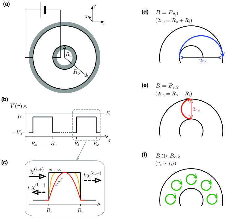
Figure 1: (a) Schematic of Corbino disk in graphene, with the inner radius $R_{\rm i}$ and the outer radius $R_{\rm o}$, contacted by two circular electrodes (dark areas). A voltage source drives a current through the disk. A separate gate electrode (not shown) allows us to tune the carrier concentration around the neutrality point. The coordinate system $(x,y,z)$ is also shown. (b) Cross section of the electrostatic potential profile given by Eq. (2) with $m\rightarrow\infty$ (i.e., the rectangular barrier) at $y=z=0$. (c) Zoom-in of a single barrier, for $x>0$, showing also the profiles for $m=2$ and $8$, with symbolic representations of the incident and reflected waves in inner electrode ($x<R_{\rm i}$) and the transmitted wave in outer electrode ($x>R_{\rm o}$) with the amplitudes $r$ and $t$ corresponding to the Fermi energy $E>0$. (d)–(f) Characteristic values of the magnetic field ${\bf B}=(0,0,B)$ separating different transport regimes. At $B=B_{c,1}$, the cyclotron diameter $2r_{c}=R_{\rm o}+R_{\rm i}$, and the particle leaving the inner lead approaches the outer lead regardless the initial direction (d). At $B=B_{c,2}$, we have $2r_{c}=R_{\rm o}-R_{\rm i}$, and only the trajectory tangent to the inner lead reaches the outer lead (e). For higher fields, classical trajectories do not contribute to the charge transport, which is possibly only if the resonance with Landau level occurs for $E\approx{}E_{n{\rm LL}}$, with $n=0,\pm{}1,\pm{}2,\dots$ (f).

II Model and methods

II.1 Dirac equation for the disk geometry

Our analysis of the device shown schematically in Fig. 1 starts from effective wave equation for Dirac fermions in graphene, near the $K$ valley,

$$\left[v_{F}\,({\boldsymbol{p}}+e{\boldsymbol{A}})\cdot{\boldsymbol{\sigma}}+V(r)\right]\Psi=E\Psi,$$ (1)

where the Fermi velocity is given by $v_{F}=\sqrt{3}\,t_{0}a/(2\hbar)$, with $t_{0}=2.7\,$eV the nearest-neighbor hopping integral and $a=0.246\,$nm the lattice parameter, ${\boldsymbol{p}}=-i\hbar\,(\partial_{x},\partial_{y})$ is the in-plane momentum operator, we choose the symmetric gauge $\mbox{\boldmath$A$}=\frac{B}{2}(-y,x)$ corresponding to the perpendicular, uniform magnetic field ${\boldsymbol{B}}=(0,0,B)$, and $\mbox{\boldmath$\sigma$}=(\sigma_{x},\sigma_{y})$, where $\sigma_{j}$ are the Pauli matrices vfhbfoo . The electrostatic potential energy in Eq. (1), $V(r)$, is given by

$$V(r)=-V_{0}\times\begin{cases}\,\frac{2^{m}|r-R_{\rm av}|^{m}}{|R_{\rm o}-R_{\rm i}|^{m}}&\text{if }\ |r\!-\!R_{\rm av}|\leqslant\frac{R_{\rm o}-R_{\rm i}}{2},\\ \,1&\text{if }\ |r\!-\!R_{\rm av}|>\frac{R_{\rm o}-R_{\rm i}}{2},\end{cases}$$ (2)

where we have defined $R_{\rm av}=(R_{\rm i}+R_{\rm o})/2$. In particular, the limit of $m\rightarrow{}\infty$ corresponds to the rectangular barrier (with a cylindrical symmetry); any finite $m\geqslant{}2$ defines a smooth potential barrier, interpolating between the parabolic ($m=2$) and rectangular shape. In principle, barrier smoothing can be regarded as a feature of a self consistent solution originating from the diffusion of carriers; we expect this feature to strongly depend on the experimental details, with graphene-on-hBN devices Zen19 showing rectangular, rather then smooth, profiles.

Symmetry of the problem allows one to look for the wave function in the form

$$\Psi_{j}(r,\varphi)=e^{i(j-1/2)\varphi}\begin{pmatrix}\chi_{a}\\ \chi_{b}e^{i\varphi}\end{pmatrix},$$ (3)

where $j=\pm{1/2},\pm{3/2},\dots$ is the total angular-momentum quantum number, the components $\chi_{a}=\chi_{a}(r)$, $\chi_{b}=\chi_{b}(r)$, and we have introduced the polar coordinates $(r,\varphi)$. Substituting the above into Eq. (1) bring us to the system of ordinary differential equations

$$\chi_{a}^{\prime} =\left(\frac{j-1/2}{r}+\frac{eBr}{2\hbar}\right)\chi_{a}+i\,\frac{E-V(r)}{\hbar{}v_{F}}\chi_{b},$$ (4)

$$\chi_{b}^{\prime} =i\,\frac{E-V(r)}{\hbar{}v_{F}}\chi_{a}-\left(\frac{j+1/2}{r}+\frac{eBr}{2\hbar}\right)\chi_{b},$$ (5)

where primes denote derivatives with respect to $r$.

II.2 Analytic solutions

For the disk area, $R_{\rm i}<r<R_{\rm o}$, Eqs. (4), (5) typically need to be integrated numerically; key details of the procedure are presented in Appendix A. Here we focus on the special case of rectangular barrier ($m=\infty$), for which some analytic solutions were reported Ryc09 ; Ryc10 ; Rec09 .

In particular, in the absence of magnetic field ($B=0$), the spinors $\chi_{j}=(\chi_{a},\chi_{b})^{T}$ corresponding to different $j$-s can be written as linear combinations Ryc09

$$\chi_{j}^{({\rm disk})}=A_{j}\begin{pmatrix}H_{j-1/2}^{(2)}(kr)\\ i\eta{}H_{j+1/2}^{(2)}(kr)\end{pmatrix}+B_{j}\begin{pmatrix}H_{j-1/2}^{(1)}(kr)\\ i\eta{}H_{j+1/2}^{(1)}(kr)\end{pmatrix},$$ (6)

where $H_{\nu}^{(1)}(\rho)$ [$H_{\nu}^{(2)}(\rho)$] is the Hankel function of the first [second] kind, $k=|E|/(\hbar{}v_{F})$, the doping sign $\eta=\mbox{sgn}\,E=\pm{}1$ (with $\eta=+1$ indicating electron doping and $\eta=-1$ indicating hole doping), and $A_{j}$, $B_{j}$, are arbitrary complex coefficients. For $B>0$, Eq. (6) is replaced by Ryc10 ; Rec09

$$\chi_{j}^{(\mathrm{disk})}=A_{j}\left(\begin{array}[]{c}\xi_{j\uparrow}^{(1)}\\ i\eta{}z_{j,1}\xi_{j\downarrow}^{(1)}\end{array}\right)+B_{j}\left(\begin{array}[]{c}\xi_{j\uparrow}^{(2)}\\ i\eta{}z_{j,2}\xi_{j\downarrow}^{(2)}\end{array}\right),$$ (7)

where $z_{j,1}=[2(j+s_{j})]^{-2s_{j}}$, $z_{j,2}=2(\beta/k^{2})^{s_{j}+1/2}$ (with $s_{j}\equiv\frac{1}{2}\mbox{sgn}\,j$, $\beta=eB/(2\hbar)$), and

$$\xi_{js}^{(\nu)}=e^{-\beta{r}^{2}/2}(kr)^{|l_{s}|}\left\{\begin{array}[]{cc}M(\alpha_{js},\gamma_{js},\beta{r}^{2}),&\nu\!=\!1,\\ U(\alpha_{js},\gamma_{js},\beta{r}^{2}),&\nu\!=\!2,\\ \end{array}\right.$$ (8)

with $l_{s}=j\mp\frac{1}{2}$ for $s=\uparrow,\downarrow$, $\alpha_{js}=\frac{1}{4}[2(l_{-s}+|l_{s}|+1)-k^{2}/\beta]$, and $\gamma_{js}=|l_{s}|+1$. $M(a,b,z)$ and $U(a,b,z)$ are the confluent hypergeometric functions Abram .

For the leads, $r<R_{\rm i}$ or $r>R_{\rm o}$, the electrostatic potential energy is constant, $V(r)=-V_{0}$. We further assume $B=0$ and $E>-V_{0}$ (electron doping) in the leads, allowing one to adapt the wave function given by Eq. (6); i.e., for the inner lead, $r<R_{\rm i}$,

$$\chi_{j}^{({\rm inner})}=\begin{pmatrix}H_{j-1/2}^{(2)}(Kr)\\ iH_{j+1/2}^{(2)}(Kr)\end{pmatrix}+r_{j}\begin{pmatrix}H_{j-1/2}^{(1)}(Kr)\\ iH_{j+1/2}^{(1)}(Kr)\end{pmatrix},$$ (9)

and for the outer lead, $r>R_{\rm o}$,

$$\chi_{j}^{({\rm outer})}=t_{j}\begin{pmatrix}H_{j-1/2}^{(2)}(Kr)\\ iH_{j+1/2}^{(2)}(Kr)\end{pmatrix},$$ (10)

where $K=|E+V_{0}|/(\hbar{}v_{F})$ and we have introduced the reflection and transmission coefficient. The first spinor in each of Eqs. (9) and (10) represents the incoming (i.e., propagating from $r=0$) wave, the second spinor in Eq. (9) represents the outgoing (propagating from $r=\infty$) wave.

II.3 Mode-matching method

Since the current-density operator following from Eq. (1), ${\boldsymbol{j}}=ev_{F}{\boldsymbol{\sigma}}$ does not involve differentiation, the mode-matching conditions for $r=R_{\rm i}$ and $r=R_{\rm o}$ reduce to the equalities for spinor components, namely

$$\chi_{j}^{({\rm inner})}(R_{\rm o})=\chi_{j}^{({\rm disk})}(R_{\rm o})\ \ \text{and }\ \chi_{j}^{({\rm disk})}(R_{\rm i})=\chi_{j}^{({\rm outer})}(R_{\rm i}).$$ (11)

The resulting formula for transmission probability for $j$-th mode becomes particularly simple upon taking the limit of heavily doped leads, $U_{0}\rightarrow{}\infty$. In particular, for $B=0$, substituting Eq. (6) into the above gives wronfoo

$$T_{j}=|t_{j}|^{2}=\frac{16}{\pi^{2}{}k^{2}{}R_{\rm i}{}R_{\rm o}}\,\frac{1}{\left[\mathfrak{D}_{j}^{(+)}\right]^{2}+\left[\mathfrak{D}_{j}^{(-)}\right]^{2}},$$ (12)

where

$$\mathfrak{D}_{j}^{(\pm)} =\mbox{Im}\left[H_{j-1/2}^{(1)}(kR_{\rm i})H_{j\mp{}1/2}^{(2)}(kR_{\rm o})\right.$$

$$\ \ \ \ \ \ \ \ \ \ \pm\left.H_{j+1/2}^{(1)}(kR_{\rm i})H_{j\pm{}1/2}^{(2)}(kR_{\rm o})\right].$$ (13)

Analogously, for $B>0$ one finds, using Eqs. (7) and (8),

$$T_{j}=|t_{j}|^{2}=\frac{16\,(k^{2}/\beta)^{|2j-1|}}{k^{2}R_{\mathrm{i}}R_{\mathrm{o}}\,(X_{j}^{2}+Y_{j}^{2})}\left[\frac{\Gamma(\gamma_{j\uparrow})}{\Gamma(\alpha_{j\uparrow})}\right]^{2},$$ (14)

where $\Gamma(z)$ is the Euler Gamma function, and

$$X_{j}=w_{j\uparrow\uparrow}^{-}+z_{j,1}z_{j,2}w_{j\downarrow\downarrow}^{-},\ \ \ Y_{j}=z_{j,2}w_{j\uparrow\downarrow}^{+}-z_{j,1}w_{j\downarrow\uparrow}^{+},$$

$$w_{jss^{\prime}}^{\pm}=\xi_{js}^{(1)}(R_{\mathrm{i}})\xi_{js^{\prime}}^{(2)}(R_{\mathrm{o}})\pm\xi_{js}^{(1)}(R_{\mathrm{o}})\xi_{js^{\prime}}^{(2)}(R_{\mathrm{i}}).$$ (15)

For $B<0$, one gets $T_{j}(B)=T_{-j}(-B)$.

Details of numerical mode-matching, applicable for smooth potentials, are given in Appendix A.

II.4 Landauer-Büttiker formalism

In case the nanoscopic system is connected to external reservoirs, characterized by the electrochemical potentials $\mu$ and $\mu+eU_{\rm eff}$ (for simplicity, the two reservoirs are considered; for more general discussion see Ref. Naz09 ), the conductance of the system is related to the transmission probabilities for normal modes ($T_{j}$-s) via

$$G(U_{\rm eff})=\frac{\langle{}I\rangle}{U_{\rm eff}}=\frac{g_{0}}{U_{\rm eff}}\int_{\mu}^{\mu+eU_{\rm eff}}d\epsilon\sum_{j}T_{j}(\epsilon),$$ (16)

where $\langle{}I\rangle$ denotes the average electric current and the zero-temperature limit is taken. The conductance quantum is $g_{0}=4e^{2}/h$, taking into account spin and valley degeneracies. $U_{\rm eff}$ denotes the effective voltage difference between the reservoirs (notice that the actual voltage applied may differ from $U_{\rm eff}$ due to charge-screening effects). Similarly, the Fano factor, relating the current variance, $\left\langle{}\left(I-\langle{}I\rangle\right)^{2}\right\rangle$, to the value $\left\langle{}\left(I-\langle{}I\rangle\right)^{2}\right\rangle_{\rm Poisson}$ one would measure in the absence of correlations between scattering events (occurring, e.g., in the tunneling limit of $T_{j}\ll{}1$ for all $j$-s), is given by

$$F(U_{\rm eff})=\frac{\left\langle{}\left(I-\langle{}I\rangle\right)^{2}\right\rangle}{\left\langle{}\left(I-\langle{}I\rangle\right)^{2}\right\rangle_{\rm Poisson}}=\frac{g_{0}}{GU_{\rm eff}}\int_{\mu}^{\mu+eU_{\rm eff}}d\epsilon\sum_{j}T_{j}(\epsilon)\left[1-T_{j}(\epsilon)\right],$$ (17)

where $\left\langle{}\left(I-\langle{}I\rangle\right)^{2}\right\rangle_{\rm Poisson}=e\langle{}I\rangle/\Delta{}t=eGU_{\rm eff}/\Delta{}t$ with $\Delta{}t$ denoting the time of measurement.

In the linear-response regime ($U_{\rm eff}\rightarrow{}0$), Eqs. (16) and (17) reduces to

$$G(U_{\rm eff}\rightarrow{}0)=g_{0}\sum_{j}T_{j},$$ (18)

and

$$F(U_{\rm eff}\rightarrow{}0)=\frac{\sum_{j}T_{j}(1-T_{j})}{\sum_{j}T_{j}},$$ (19)

where $T_{j}=T_{j}(\mu)$. For the disk geometry, summation range is limited by the number of propagating modes in the inner lead, $|j|\leqslant{}j_{\rm max}=\lfloor{}KR_{\rm i}\rfloor-\frac{1}{2}$ with $\lfloor{}x\rfloor$ denoting the floor function of $x$. (For heavily-doped leads, $j_{\rm max}\rightarrow{}\infty$.)

As a notable example, we consider the zero-doping limit ($\mu\rightarrow{}0$). In such a case, Eq. (14) simplifies to Ryc10 ; Kat10

$$T_{j}(\mu\rightarrow{}0)=\frac{1}{\cosh^{2}[(j+\Phi/\Phi_{0})\ln(R_{\rm o}/R_{\rm i})]},$$ (20)

where $\Phi=\pi(R_{\mathrm{o}}^{2}-R_{\mathrm{i}}^{2})B$ is the flux piercing the disk area and we have defined $\Phi_{0}=2\,(h/e)\ln(R_{\rm o}/R_{\rm i})$. Assuming the narrow-disk range, $R_{\rm o}\approx{}R_{\rm i}$, we can approximate the sums occurring in Eqs. (18) and (19) by integrals, obtaining

$$G\approx{}G_{\rm diff}=\frac{2\pi{}\sigma_{0}}{\ln(R_{\rm o}/R_{\rm i})}\ \ \ \ \text{and }\ \ \ \ F\approx{}F_{\rm diff}=\frac{1}{3}.$$ (21)

The above reproduces pseudodiffusive conductance and the shot-noise power for a disk geometry Ryc09 . For larger $R_{\rm o}/R_{\rm i}$, both characteristics are predicted to show approximately sinusoidal conductance oscillations with the field $B$ Ryc10 ; Kat10 ; Ryc12 .

The case of doped disk, for which one may expect to observe some features of the sub-Sharvin charge transport Ryc21b ; Ryc22 , is discussed next.

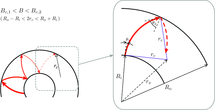
Figure 2: Propagation between consecutive scatterings on interfaces at $r=R_{\rm i}$ and $r=R_{\rm o}$ in a uniform magnetic field $B_{c,1}<B<B_{c,2}$. A zoom-in shown an arc of single cyclotron orbit centered at $r=r_{x}$, with its radii $r_{c}$, and incident angles $\theta_{1}$ (for $r=R_{\rm i}$) and $\theta_{2}$ (for $r=R_{\rm o}$).

III Approximate conductance and Fano factor at the magnetic field

Before calculating the conductance $G$ and Fano factor $F$ within the mode-matching method described in Sec. II, we first present the approximating formulas for incoherent transport, obtained by adapting the derivation of Ref. Ryc22 for the $B>0$ case.

III.1 Corbino disk in graphene as a double barrier

A key step in the derivation is to observe that, in the multimode regime ($kR_{\rm i}\gg{}1$) for which one can consider well-defined trajectories, the disk symmetry cause that incident angles $\theta_{1}$ and $\theta_{2}$, corresponding to the interfaces at $r=R_{\rm i}$ and $r=R_{\rm o}$ (see Fig. 2) remain constant (up to a sign) after multiple scatterings. Therefore, one can apply the double-contact formula for incoherent transmission Dat97 ; intfoo , namely

$$\left\{T\right\}_{\rm incoh} =\frac{1}{2\pi}\int_{-\pi}^{\pi}d\phi\,\frac{T_{1}T_{2}}{2-T_{1}-T_{2}+T_{1}{}T_{2}-2\sqrt{(1-T_{1}{})(1-T_{2})}\cos{\phi}}=\frac{T_{1}T_{2}}{T_{1}+T_{2}-T_{1}T_{2}},$$ (22)

where the transmission probabilities $T_{1}$, $T_{2}$, corresponding to a potential step of infinite height, are given by

$$T_{l}=\frac{2\cos\theta_{l}}{1+\cos\theta_{l}},\ \ \ \ \ \ l=1,2,$$ (23)

and $\phi$ is assumed to be a random phase acquired during the propagation between $r=R_{\rm i}$ and $r=R_{\rm o}$ (or vice versa). Similarly, we calculate the incoherent squared transmission, useful when evaluating the Fano factor,

$$\left\{T^{2}\right\}_{\rm incoh} =\frac{1}{2\pi}\int_{-\pi}^{\pi}d\phi\,\left(\frac{T_{1}T_{2}}{2-T_{1}-T_{2}+T_{1}{}T_{2}-2\sqrt{(1-T_{1}{})(1-T_{2})}\cos{\phi}}\right)^{2}=\frac{(T_{1}T_{2})^{2}(2-T_{1}-T_{2}+T_{1}T_{2})}{(1+T_{1}T_{2}-T_{1}T_{2})^{3}}.$$ (24)

Next, the incoherent conductance in the linear-response regime is evaluated by inserting $\left\{T\right\}_{\rm incoh}$ (22) into Eq. (18),

$$G_{\rm incoh}=G_{\rm Sharvin}\left\langle{}\left\{T\right\}_{\rm incoh}\right\rangle_{u=\sin\theta_{1}},$$ (25)

with

$$G_{\rm Sharvin}=2g_{0}kR_{\rm i}.$$ (26)

For the Fano factor, one can analogously derive from Eq. (19)

$$F_{\rm incoh}=1-\frac{\left\langle{}\left\{T^{2}\right\}_{\rm incoh}\right\rangle_{u=\sin\theta_{1}}}{\left\langle{}\left\{T\right\}_{\rm incoh}\right\rangle_{u=\sin\theta_{1}}}.$$ (27)

The summation over $2kR_{\rm i}$ modes is approximated in Eqs. (25), (27) by averaging over the variable $u=\sin\theta_{1}$, within the range of $-1\leqslant{}u\leqslant{}1$. Explicitly,

$$\left\langle{}\left\{T^{n}\right\}_{\rm incoh}\right\rangle_{u=\sin\theta_{1}}=\frac{1}{2}\int_{u_{c}}^{1}du\left\{T^{n}\right\}_{\rm incoh},\ \ \ \ n=1,2,$$ (28)

where the lower integration limit ($u_{c}$) is defined via the value of $\sin\theta_{1}$, below which the trajectory cannot reach the outer interface ($r=R_{\rm o}$). (In other words, for $u=\sin\theta_{1}<u_{c}$, the geometric derivation to be presented below leads to $|\sin\theta_{2}|>1$.)

The missing elements, necessary to calculate $\left\langle{}\left\{T^{n}\right\}_{\rm incoh}\right\rangle_{u=\sin\theta_{1}}$ in Eq. (28) is the dependence of $\theta_{2}$ on $\theta_{1}$ and $B$ [see Eqs. (22), (23), and (24)], as well as the dependence of $u_{c}$ on $B$. Since we have assumed constant electrostatic potential energy in the disk area, the trajectory between subsequent scatterings (see Fig. 2) forms an arc, with the constant radii

$$r_{c}=\hbar{}k/(eB)=|E|/(v_{F}eB),$$ (29)

(i.e., the cyclotron radius for massless Dirac particle at $B>0$), centered at the distance $r_{x}$ from the origin. Now, solving the two triangles with a common edge $r_{x}$ (dashed line) and the opposite vertices in two scattering points, we find

$$r_{x}^{2}=R_{\rm i}^{2}+r_{c}^{2}+2R_{\rm i}{}r_{c}\sin\theta_{1}$$ (30)

(for the triangle containing a scattering point at $r=R_{\rm i}$), and

$$r_{x}^{2}=R_{\rm o}^{2}+r_{c}^{2}-2R_{\rm o}{}r_{c}\sin\theta_{2}$$ (31)

(for the triangle containing a scattering point at $r=R_{\rm o}$). Together, Eqs. (30) and (31) lead to

$$\sin\theta_{2}=\frac{R_{\rm o}^{2}-R_{\rm i}^{2}-2R_{\rm i}r_{c}u}{2R_{\rm o}r_{c}}.$$ (32)

Subsequently, the value of $u_{c}$ in Eq. (28) is given by

$$u_{c}=\begin{cases}-1,&\text{if }\ B\leqslant{}B_{c,1}\\ \frac{R_{\rm o}^{2}-R_{\rm i}^{2}}{2R_{\rm i}r_{c}}-\frac{R_{\rm o}}{R_{\rm i}},&\text{if }\ B_{c,1}<B\leqslant{}B_{c,2}\\ 1,&\text{if }\ B>B_{c,2}\\ \end{cases},$$ (33)

where we have additionally defined

$$B_{c,m}=\frac{2\hbar{}k}{e\left[R_{\rm o}-(-1)^{m}{}R_{\rm i}\right]},\ \ \ \ \ m=1,2.$$ (34)

III.2 The zero-field limit

Typically, averages occurring in Eqs. (25) and (27) need to be evaluated numerically. Analytic expressions are available, e.g., for zero magnetic field Ryc22

$$G_{\rm incoh}(B\!\rightarrow{}\!0) =G_{\rm Sharvin}\,\frac{(2a+\frac{1}{a})\arcsin{}a+3\sqrt{1-a^{2}}-\frac{\pi}{2}(a^{2}+2)}{1-a^{2}},$$ (35)

$$F_{\rm incoh}(B\!\rightarrow{}\!0) =\frac{2a\sqrt{1-a^{2}}(53+279a^{2}+88a^{4})-3\pi{}a(12+82a^{2}+45a^{4}+a^{6})+6(1+45a^{2}+82a^{4}+12a^{6})\arcsin{}a}{6(1-a^{2})^{2}\left[\pi{}a(a^{2}+2)-6a\sqrt{1-a^{2}}-2(2a^{2}+1)\arcsin{}a\right]},$$ (36)

where we have defined the inverse radii ratio $a=R_{\rm i}/R_{\rm o}$.

III.3 The zero-conductance limit

In the this paper, we focus on the limit of $B\rightarrow{}B_{c,2}-$ (i.e., $B$ approaching $B_{c,2}$ from below), for which $G_{\rm incoh}\rightarrow{}0$. Introducing the dimensionless $0<\varepsilon\ll{}1$, one can express the cyclotron diameter, see Eq. (29), as

$$2r_{c}=R_{\rm o}-R_{\rm i}+\varepsilon{}\left(R_{\rm o}-R_{\rm i}\right).$$ (37)

In turn, the value $u_{c}$, see Eq. (33), can be approximated (up to the leading order in $\varepsilon$) as

$$u_{c}\approx{}1-\varepsilon\left(1+\frac{R_{\rm o}}{R_{\rm i}}\right).$$ (38)

It is now convenient to define the variable

$$\alpha=\frac{1-u}{\varepsilon\left(1+{R_{\rm o}}/{R_{\rm i}}\right)},$$ (39)

such that the integration over $u_{c}\leqslant{}u\leqslant{}1$, occurring when evaluating $\left\langle{}\left\{T^{n}\right\}_{\rm incoh}\right\rangle_{u=\sin\theta_{1}}$ from Eq. (28), can be replaced by integration over $1\geqslant{}\alpha\geqslant{}0$. Transmission probabilities ($T_{1}$, $T_{2}$) for the interfaces at $r=R_{\rm i}$ and $r=R_{\rm o}$, see Eqs. (22), (23), (24) and (32), can now be approximated as

$$T_{1} \approx 2\sqrt{2\alpha\left(1+{\scriptstyle\frac{1}{a}}\right)}\,\varepsilon^{1/2},$$ (40)

$$T_{2} \approx 2\sqrt{2(1-\alpha)\left(1+{a}\right)}\,\varepsilon^{1/2},$$ (41)

where we have used $a=R_{\rm i}/R_{\rm o}$ again.

Using the above expressions, we can now rewrite the averages occurring in Eq. (28), up to the leading order in $\varepsilon$ again, as follows

$$\left\langle{}\left\{T\right\}_{\rm incoh}\right\rangle_{u} =\frac{G_{\rm incoh}}{G_{\rm Sharvin}}\approx\frac{2\left(1+\frac{1}{a}\right)}{\sqrt{2}}\,\varepsilon^{3/2}\int_{0}^{1}{}d\alpha\frac{\sqrt{\alpha(1+\frac{1}{a})}\sqrt{(1-\alpha)(1+a)}}{\sqrt{\alpha(1+\frac{1}{a})}+\sqrt{(1-\alpha)(1+a)}},$$ (42)

$$\left\langle{}\left\{T^{2}\right\}_{\rm incoh}\right\rangle_{u} \approx\frac{2\left(1+\frac{1}{a}\right)}{\sqrt{2}}\,\varepsilon^{3/2}\int_{0}^{1}{}d\alpha\frac{\alpha(1-\alpha)\left(2+\frac{1}{a}+a\right)}{\left[\sqrt{\alpha(1+\frac{1}{a})}+\sqrt{(1-\alpha)(1+a)}\right]^{3}}.$$ (43)

Remarkably, both quantities decays as $\propto{}\varepsilon^{3/2}$, but their ratio, occurring in Eq. (27) for the Fano factor, remains constant (for a given $a$). The integrals in Eqs. (42) and (43) can be calculated analytically, leading to

$$F_{\rm incoh}(B\!\rightarrow{}\!B_{c,2}-) =1-\left\{4\sqrt{a}+39a-58a^{3/2}-23a^{2}-23a^{5/2}-58a^{3}+39a^{7/2}+4a^{4}\right.$$

$$\hskip 34.44434pt+\left.\left(69a^{2}-18a^{3}-18a\right)\sqrt{1+a}\,\mbox{artanh}\left(\frac{\sqrt{a}}{\sqrt{1+a}}\right)\right.$$

$$\hskip 34.44434pt+\left.\left(69a^{2}-18a-18a^{3}\right)\sqrt{1+a}\,\mbox{artanh}\left(\frac{1}{\sqrt{1+a}}\right)\right\}$$

$${\Big{/}}\left\{(1+a)^{3}\left(1+\sqrt{a}\right)\left(1-3\sqrt{a}+a\right)+3a(1+a)^{5/2}\,\mbox{artanh}\left[\frac{(1+\sqrt{a})\sqrt{1+a}}{1+\sqrt{a}+a}\right]\right\}.$$ (44)

Numerical values of $F_{\rm incoh}(B\!\rightarrow{}\!0)$ and $F_{\rm incoh}(B\!\rightarrow{}\!B_{c,2}-)$ for selected $a=R_{\rm i}/R_{\rm o}$ are given in Table 1. For $F_{\rm incoh}(B\!\rightarrow{}\!B_{c,2}-)$, we see that the poissonian value of $F_{\rm incoh}=1$, which one could expect due to the vanishing conductance, is reconstructed only for $a\rightarrow{}0$ (i.e., for $R_{\rm o}\gg{}R_{\rm i}$). For finite radii ratios, nontrivial values of $0<F_{\rm incoh}<1$ occurs. Remarkable, for moderate disk proportions ($a\geqslant{}0.5$), $F_{\rm incoh}(B\!\rightarrow{}\!B_{c,2}-)$ shows very weak dependence on $a$, decaying by less then $2\%$ (from $F_{\rm incoh}\approx{}0.56$ at $a=0.5$ to $F_{\rm incoh}\approx{}0.55$ for $a\rightarrow{}1$, with $a\rightarrow{}1$ representing the narrow-disk limit of $R_{\rm o}\approx{}R_{\rm i}$).

For this reason, in the following numerical analysis, we fixed the disk radii ratio at $a=0.5$ (i.e., $R_{\rm o}=2R_{\rm i}$). We also stress that the derivation presented above, holds true for the parameter $\varepsilon\rightarrow{}0+$, quantifying the ratio of cyclotron diameter $2r_{c}$ to radii difference $R_{\rm o}-R_{\rm i}$, see Eq. (37). Therefore, it is irrelevant whether one increases the magnetic field at a fixed chemical potential, or reduces the chemical potential at a fixed $B>0$ (as long as the system stays in a multimode range, $kR_{\rm i}\gg{}1$).

Table 1: Selected numerical values of $F_{\rm incoh}(B\!\rightarrow{}\!0)$, see Eq. (36), and $F_{\rm incoh}(B\!\rightarrow{}\!B_{c,2}-)$, see Eq. (44). Box marks the values for $a=0.5$ (i.e., $R_{\rm o}=2R_{\rm i}$) to be compared with the results following from numerical simulations of quantum transport presented Sec. IV.

$\ a=R_{\rm i}/R_{\rm o}\$	$\ F_{\rm incoh}(B\rightarrow{}0)\$	$\ F_{\rm incoh}(B\rightarrow{}B_{c,2}-)\$
0	0.106528	1
0.1	0.106705	0.630994
0.2	0.107239	0.591829
0.3	0.108136	0.573885
0.4	0.109409	0.563905
0.5	0.111074	0.557898
0.6	0.113151	0.554178
0.7	0.115663	0.551894
0.8	0.118619	0.550565
0.9	0.121963	0.549899
1.0	0.125000	0.549708

IV Results and discussion

Main doubt arising when we consider the applicability of Eq. (44) for real quantum systems concerns the possible role of evanescent waves, totally neglected in our derivation. Obviously, they should not play an important role when the system is highly conducting (such as in the zero-field case Ryc22 ); however, since the Fano factor is determined by the ratio of two cumulants, both vanishing for sufficiently high field, it is not fully clear which contribution (from propagating or from evanescent modes) would govern the value of $F$ for $B\rightarrow{}B_{c,2}$? On the other hand, resonances with Landau levels are not expect to play a significant role, as they form very narrow transmission peaks, contributions of which get immediately smeared out beyond the linear-response regime.

In the remaining parts of the paper, compare the results of computer simulation of quantum transport through the disk in graphene, with the predictions for incoherent scattering presented in Sec. III, in attempt to propose an experimental procedure allowing one to extract the nontrivial value of $F\approx{}0.55$ from the data plagued with other contributions.

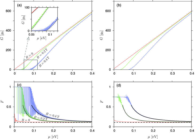
Figure 3: (a,b) Conductance and (c,d) the Fano factor for the Corbino disk in graphene with the radii $R_{\rm o}=2R_{\rm i}=1000\,$nm and the rectangular potential barrier (i.e., $V_{0}\rightarrow{}\infty$ and $m\rightarrow{}\infty$ in Eq. (2)) displayed as functions of the chemical potential. The values of magnetic field are $B=0$ (red solid lines in all plots), $B=0.2\,$T (green solid lines), and $B=0.4\,$T (blue solid lines). Inset in (a) is a zoom-in, with black dashed lines depicting the incoherent conductance, see Eq. (25). (a) and (c) show the linear-response results, see Eqs. (18) and (19); the datasets in (b) and (d) are obtained from Eqs. (16) and (17) with $U_{\rm eff}=0.01\,$V. Remaining lines in (c,d) [black solid, black dotted, and black dashed] mark the incoherent Fano factor, see Eq. (27); the values of magnetic field are specified for lines in (c), and are the same in (d). (For $B=0$, horizontal lines mark $F_{\rm incoh}(B\rightarrow{}0)=0.111074$ corresponding to $R_{\rm o}=2R_{\rm i}$, see Table 1.)

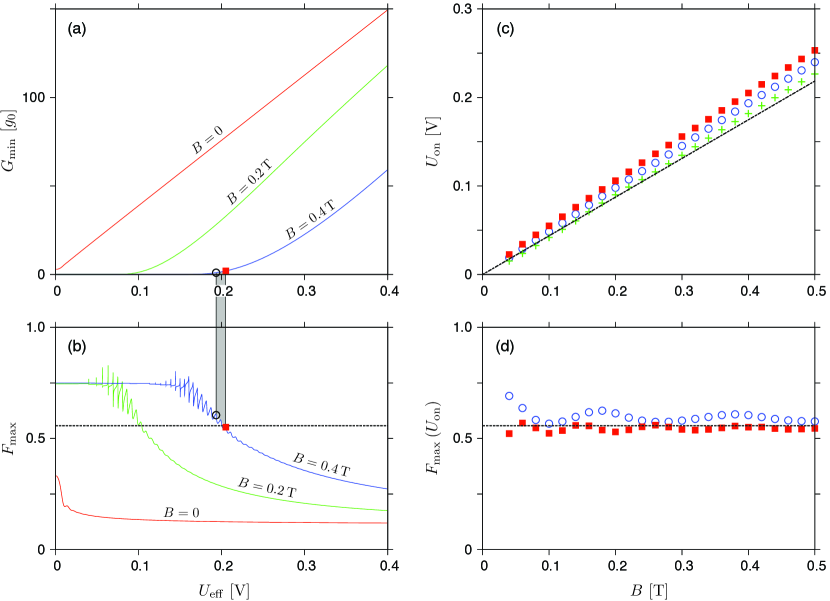
Figure 4: (a,b) Minimal conductivity and maximal Fano factor, see Eqs. (16) and (17), corresponding to the chemical potential fixed at $\mu=-eU_{\rm eff}/2$, versus the effective voltage. The magnetic field is specified for each line. (c) The activation voltage, defined via $G_{\rm min}(U_{\rm on}^{(1)})=g_{0}$ [blue open circles], $G_{\rm min}(U_{\rm on}^{(2)})=2g_{0}$ [red solid squares], or obtained from scaling according to Eq. (46) [green crosses], displayed versus the magnetic field. (d) The Fano factor corresponding to $U_{\rm eff}=U_{\rm on}$ shown in (c). Horizontal dashed lines in (b,d) mark the value of $F_{\rm incoh}(B\rightarrow{}B_{c,2}-)=0.557898$ for $R_{\rm o}=2R_{\rm i}$ (see Table 1). Dashed line in (c) depicts the approximation given in Eq. (45). The remaining system parameters are same as in Fig. 3.

IV.1 The rectangular barrier of an infinite height

As a first numerical example, we took the limit of $V_{0}\rightarrow{}\infty$ and $m\rightarrow{}\infty$ in Eq. (2), for which close-form expressions for transmission probabilities were presented in Sec. II.

In Fig. 3, we compare the linear-response conductance $G(U_{\rm eff}\rightarrow{}0)$, see Eq. (18), with $G(U_{\rm eff})$ calculated from Eq. (16) for a small but nonzero value of $U_{\rm eff}=0.01\,$V, both displayed as functions of the chemical potential. Also in Fig. 3, same comparison is presented for the Fano factor $F(U_{\rm eff})$ [see Eqs. (19) and (17)]. It easy to see that prominent, aperiodic oscillations visible for both charge-transfer cumulants in the $U_{\rm eff}\rightarrow{}0$ limit are significantly reduced even for small $U_{\rm eff}>0$. In fact, for $U_{\rm eff}=0.01\,$V and $B>0$, the values of $F_{\rm incoh}$ calculated from Eq. (27) [black lines] are closely followed by $F(U_{\rm eff})$ obtained from the numerical mode-matching, as long as the former can be defined, i.e., for $B<B_{c,2}$ at a given $\mu$. We further notice that the value of $\mu$ for which $B\approx{}B_{c,2}$ and $F(U_{\rm eff})\approx{}0.56$ corresponds to $G(U_{\rm eff})\sim{}g_{0}$ (up to the order of magnitude). For smaller $\mu$, such that $B>B_{c,2}$ and $F_{\rm incoh}$ is undefined, $F(U_{\rm eff})$ saturates near the value $\approx{}0.75$, apparently below the poissonian limit of $F=1$.

To better understand the nature of the results we now, in Fig. 4, go further beyond the linear-response regime, calculating $G(U_{\rm eff})$ and $F(U_{\rm eff})$ for $\mu=-eU_{\rm eff}/2$ (notice that for an infinite rectangular barrier we have the particle-hole symmetry, and both cumulants are even upon $\mu\leftrightarrow{}-\mu+eU_{\rm eff}$) and displaying them as functions of $U_{\rm eff}$.

We further introduce the activation voltage $U_{\rm on}=U_{\rm on}(B)$, meaning of which can be understood as follows. The cyclotron diameter, see Eq. (29), naturally defines the range of energies for which $2r_{c}(E)<R_{\rm o}-R_{\rm i}$ and the system shows $G\approx{}0$ (up to the evanescent modes). On the other hand, as we have set $\mu=-eU_{\rm eff}/2$, the effective voltage defines the energy range of $|E|\leqslant{}eU_{\rm eff}/2$, being the integration interval in Eqs. (16) and (17). In turn, $G(U_{\rm eff})>0$ is expected for $U_{\rm eff}\geqslant{}U_{\rm on}$, a value of which can be approximated as

$$U_{{\rm on},{\rm incoh}}=v_{F}{}B\left(R_{\rm o}-R_{\rm i}\right),$$ (45)

where we have simply rewrite equality $2r_{c}(eU_{\rm on})=R_{\rm o}-R_{\rm i}$ neglecting the evanescent modes.

When looking on the conductance spectra illustrated in Fig. 4(a) we see, for $B>0$, a wide range of lower $U_{\rm eff}$ for which $G\approx{}0$, attached (via a cusp region) to the range of (approximately linearly) increasing $G$. In order to determine the value of $U_{\rm on}(B)$ directly from the conductance spectra $G(U_{\rm eff})$, we find numerically the value of $U_{\rm on}^{(1)}$ such that $G(U_{\rm on}^{(1)})=g_{0}$, and $U_{\rm on}^{(2)}$ such that $G(U_{\rm on}^{(2)})=2g_{0}$, see the datapoints in Fig. 4(a). Then, the linear extrapolation is performed to obtain

$$U_{\rm on}^{(0)} =U_{\rm on}^{(1)}-\left(U_{\rm on}^{(2)}-U_{\rm on}^{(1)}\right)\frac{G(U_{\rm on}^{(1)})}{G(U_{\rm on}^{(2)})-G(U_{\rm on}^{(1)})}$$

$$=2U_{\rm on}^{(1)}-U_{\rm on}^{(2)},$$ (46)

such that $G(U_{\rm on}^{(0)})\approx{}0$. The resulting values of $U_{\rm on}^{(i)}$, depicted in Fig. 4(c) [datapoints], stay close to $U_{{\rm on},{\rm incoh}}$ obtained from Eq. (45) [dashed line].

Remarkably, the values of the Fano factor corresponding to $U_{\rm eff}=U_{\rm on}^{(i)}$, $i=1,2,$ see Fig. 4(b), are close to $F_{\rm incoh}(B\rightarrow{}B_{c,2}-)\approx{}0.56$. Similar observation applies for all studied values of $B\leqslant{}0.5\,$T, see Fig. 4(d); a typical deviation does not exceed $5\%$.

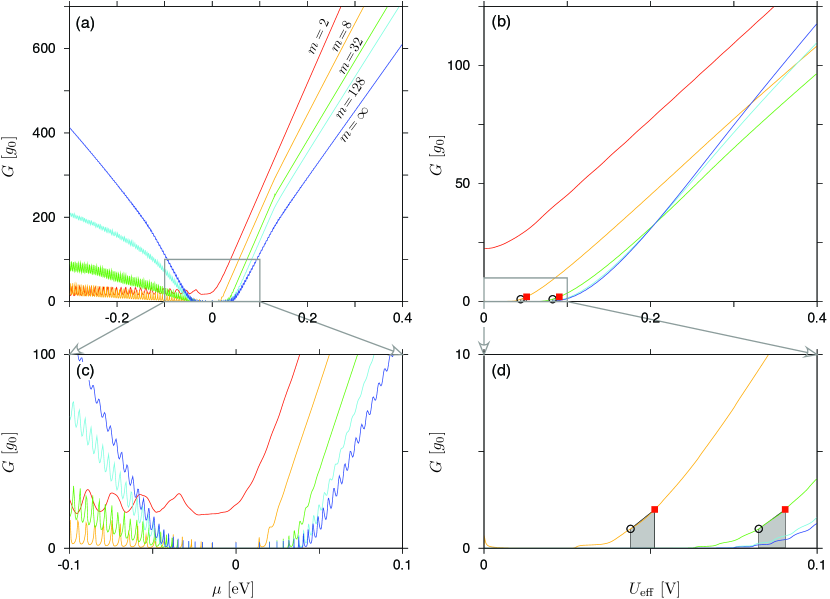
Figure 5: (a) Linear-response conductance as a function of the chemical potential and (b) finite-voltage conductance, for $\mu=-eU_{\rm eff}/2$, as a function of the voltage. The magnetic field is $B=0.2\,$T for all plots. The disk radii are the same as in Fig. 3, but the barrier height, see Eq. (2)), is now fixed at $V_{0}=t_{0}/2=1.35\,$eV; the parameter $m$ is specified for each line. (c,d) Zoom-in, for low energies, with same datasets as in (a,b). Datapoints in (b,d) mark the values of $G(U_{\rm on}^{(i)})=ig_{0}$, $i=1,2,$ defining the activation voltages $U_{\rm eff}=U_{\rm on}^{(i)}$.

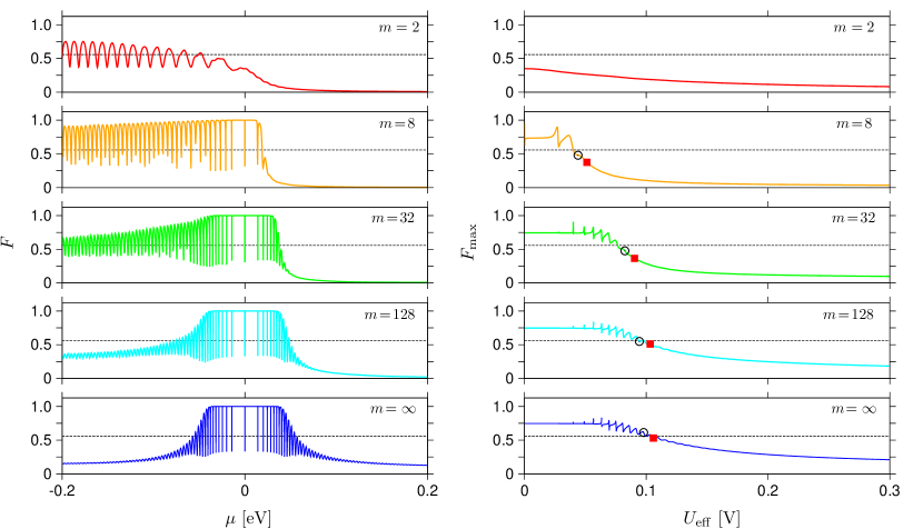
Figure 6: Left: Linear-response Fano factor as a function of the chemical potential. Right: Finite-voltage Fano factor, for $\mu=-eU_{\rm eff}/2$, as a function of the voltage. The magnetic field is $B=0.2\,$T for all plots, the value of exponent $m$ is specified at each plot, and remaining parameters are same as in Fig. 5. Horizontal line at each plot marks the value of $F_{\rm incoh}(B\rightarrow{}B_{c,2}-)=0.557898$, see Table 1. Datapoints (right) mark the values of $F(U_{\rm on}^{(i)})$, $i=1,2,$ corresponding to activation voltages $U_{\rm eff}=U_{\rm on}^{(i)}$, for which $G(U_{\rm on}^{(i)})=ig_{0}$ (see also Fig. 5).

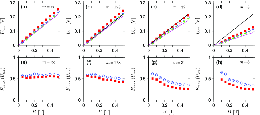
Figure 7: (a–d) The activation voltage (for the definition, see Fig. 4) and (e–h) the corresponding Fano factor for $\mu=-eU_{\rm eff}/2$, displayed as functions of the magnetic field [datapoints]. The value of exponent $m$ is specified at each plot; remaining parameters are same as in Fig. 5. Lines in (a–d) depict the approximation given by Eq. (47) [purple solid] and Eq. (45) [black dashed] coinciding in the $m\rightarrow{}\infty$ limit. Horizontal lines in (e–h) mark the value of $F_{\rm incoh}(B\rightarrow{}B_{c,2}-)=0.557898$, see Table 1.

IV.2 Smooth potential barriers

In this subsection, we extend our numerical analysis onto smooth potential barriers, defined by choosing $2\leqslant{}m<\infty$ in Eq. (2). Moreover, the barrier height is now finite, i.e., $V_{0}=t_{0}/2=1.35\,$eV, being not far from the results of some first-principles calculations for graphene-metal structures Gio08 ; Cus17 . According to our best knowledge such a model, first proposed in Ref. Ryc21b , seems to be the simplest providing qualitatively correct description of the conductance-spectrum asymmetry observed in existing experiments Pet14 ; Kam21 ; Kum22 , in which the conductance for $\mu<0$ is noticeably suppressed, comparing to the $\mu>0$ range, due to the presence of two circular p-n junctions in the former case. (Such a feature is also correctly reproduced by a simpler model assuming the trapezoidal potential barrier Par21 , allowing a fully analytic treatment, but this approach produces an artificial conductance maximum near $\mu=0$.)

The conductance spectra for five selected values of $m$ are displayed in Fig. 5, both for the linear-response regime [see Figs. 5(a,c)] and beyond [Figs. 5(b,d)]. This time, we have limited out presentation a single value of magnetic field, i.e., $B=0.2\,$T. It must be notice that finite value of $V_{0}$ results in small, but visible spectrum asymmetry also for $m=\infty$.

The finite-voltage results, $G(U_{\rm eff})$ at $\mu=-eU_{\rm eff}/2$, allows as to determine the activation voltage, $U_{\rm on}(B)$, in a similar manner as for an infinite-barrier case (see previous subsection). When attempting to apply the incoherent-scattering approximation to smooth potentials, some modification is required for Eq. (45), which now can be rewritten as

$$U_{{\rm on},{\rm incoh}}=v_{F}{}BL_{\rm diff}(m).$$ (47)

In the above, we have introduced the $m$-dependent effective sample length given by Ryc21b ; Ryc22

$${L_{\rm diff}(m)}=|R_{\rm o}-R_{\rm i}|\left(\frac{\hbar{}v_{F}}{|R_{\rm o}-R_{\rm i}|V_{0}}\right)^{1/m},$$ (48)

which reduces to $L_{\rm diff}(\infty)=R_{\rm o}-R_{\rm i}$ for a rectangular barrier, and gives $L_{\rm diff}(m=2)\ll{}R_{\rm o}-R_{\rm i}$ for the parabolic case. In brief, Eq. (48) can be derived by imposing $V(\pm{}L_{\rm diff}/2)=-E_{\rm diff}$, where $E_{\rm diff}$ denotes the value of Fermi energy, above which Sharvin conductance overrules the pseudodiffusive conductance, namely,

$$E_{\rm diff}=\frac{\hbar{}v_{F}}{R_{\rm o}-R_{\rm i}}\approx{}1\,\text{meV}\ \ \ \text{for}\ \ \ R_{\rm o}-R_{\rm i}=500\,\text{nm}.$$ (49)

In Fig. 6 we show the Fano factor, for same five values of $m$ as previously used for the conductance (see Fig. 5), and $B=0.2\,$T, as a function $\mu$ in the linear-response limit ($U_{\rm eff}\rightarrow{}0$), as well as a function $U_{\rm eff}$ for $\mu=-U_{\rm eff}/2$ (see left or right side of Fig. 6, respectively). Again, the aperiodic oscillations almost vanish when entering the nonlinear response regime; in fact, the shape of $F_{\rm max}(U_{\rm eff})$ appears to be much less sensitive to the value of $m$ than the linear-response $F(\mu)$. Datapoints on the right side of Fig. 6, identifying the values of $F(U_{\rm on}^{(i)})$, $i=1,2,$ such that $G(U_{\rm on}^{(i)})=ig_{0}$ (see Fig. 5), are available starting from $m=8$ (although the deviation from $F_{\rm incoh}(B\rightarrow{}B_{c,2}-)\approx{}0.56$ is significant in such a case), whereas strong asymmetry of $F(\mu)$ is visible up to $m=32$.

The values of $U_{\rm on}^{(i)}$ and the corresponding $F(U_{\rm on}^{(i)})$, for the magnetic fields up to $B\leqslant{}0.5\,$T, are displayed in Fig. 7. It can be noticed that the voltages $U_{\rm on}^{(i)}$, see datapoints in Figs. 7(a–d), show relatively good agreement with the approximation given by Eq. (47) [purple solid lines]; in fact, significant deviation from Eq. (45) relevant for the rectangular barrier [black dashed lines] can be noticed for $m=8$ only. On the contrary, corresponding Fano factors $F(U_{\rm on}^{(i)})$, see datapoints in Figs. 7(e–h), stay close to the value of $F_{\rm incoh}(B\rightarrow{}B_{c,2}-)\approx{}0.56$ only for $m=\infty$ and $m=128$, showing that the incoherent treatment of the shot-noise power, which we put forward in Sec. III, is applicable only if the potential profiles is close to (but not necessarily perfectly matching) the rectangular shape.

V Conclusions

We have put forward an analytic description of the shot-noise power in graphene-based disks in high magnetic field and doping. Assuming the incoherent scattering of Dirac fermions between two potential steps of an infinite height, both characterized by a priori nonzero transmission probability due to the Klein tunneling, we find that vanishing conductance should be accompanied by the Fano factor $F\approx{}0.56$, weakly-dependent on the disk proportions.

Next, the results of analytic considerations are confronted with the outcome of computer simulations, including both rectangular and smooth shapes of the electrostatic potential barrier in the disk area. Calculating both linear-response and finite-voltage transport cumulants, within the zero-temperature Landauer-Büttiker formalism, we point out that the role of evanescent waves (earlier ignored in the analytic approach) is significant in the linear-response regime, however, one should able to detect the quasi-universal $F\approx{}0.56$ noise in a properly designed experiment going beyond the linear response regime. To achieve this goal, the following procedure is proposed: First, the activation voltage (for a fixed magnetic field) needs to be determined, by finding a cusp position on the conductance-versus-voltage plot, above which the conductance grows fast with the voltage (the average chemical potential is controlled by the gate such that the conductance is minimal for a given voltage). Having the activation voltage determined, one measures the noise for such a voltage, expecting the Fano factor to be close to $F\approx{}0.56$.

We expect that the effect we describe should be observable in ultraclean samples and sub-kelvin temperatures (such as in Ref. Zen19 ); for higher temperatures, hydrodynamic effects may noticeably alter the measurable quantities Kum22 . Since the noise-related characteristics seem to be generally more sensitive to the potential shape then the conductance (or the thermoelectric properties earlier discussed in Ref. Ryc23 ), the experimental study following the scenario presented here may be a suitable way to check whether the flat-potential area of a mesoscopic size is present or not in a given graphene-based structure.

Appendix A Numerical mode matching for smooth potentials

Here we summarize the numerical approach earlier presented in Ref. Ryc23 .

In a typical situation, system of ordinary differential equations for spinor components $(\chi_{a},\chi_{b})$, see Eqs. (4) and (5), needs to be integrated numerically for all $j$-s. In order to reduce round-off errors that may occur in finite-precision arithmetics due to exponentially growing (or decaying) solutions, one can divide the full interval, $R_{\rm i}<r<R_{\rm o}$, into $M$ parts, bounded by

$$R_{c}^{(l)} =R_{\rm i}+l\frac{R_{\rm o}-R_{\rm i}}{M}<r<R_{c}^{(l+1)},$$

$$\text{with }\ \ l=0,1,\dots,M-1.$$ (50)

(In particular, $R_{c}^{(0)}=R_{\rm i}$ and $R_{c}^{(M)}=R_{\rm o}$.)

The wave function in the disk area $\chi_{j}^{({\rm disk})}$ is now given by a series of functions $\left\{\chi_{j}^{(l)}\right\}$ for $M$ consecutive intervals given by Eq. (A). For the $l$-th interval,

$$\chi_{j}^{(l)}=A_{j}^{(l)}\chi_{j}^{(l),{\rm I}}+B_{j}^{(l)}\chi_{j}^{(l),{\rm II}},$$ (51)

where $\chi_{j}^{(l),{\rm I}}$, $\chi_{j}^{(l),{\rm II}}$ are two linearly independent solutions obtained by integrating Eqs. (4), (5) with two different initial conditions, $\left.\chi_{j}^{(l),{\rm I}}\right|_{r=R_{\rm i}^{(l)}}=(1,0)^{T}$ and $\left.\chi_{j}^{(l),{\rm II}}\right|_{r=R_{\rm i}^{(l)}}=(0,1)^{T}$. $A_{j}^{(l)}$ and $B_{j}^{(l)}$ are complex coefficients (to be determined later).

In particular, for $R_{\rm o}=2R_{\rm i}=1000\,$nm and $B<0.5\,$T considered in this paper, it is sufficient to set $M=20$ and employ a standard fourth-order Runge-Kutta (RK4) algorithm with a spatial step of $0.5\,$pm. (For such a choice, the output numerical uncertainties of transmission probabilities $T_{j}$ are smaller then $10^{-7}$.)

The matching conditions for the $M+1$ interfaces at $r=R_{\rm i}$, $r=R_{c}^{(1)}$, …, $r=R_{c}^{(M-1)}$, and $r=R_{\rm o}$, can now be written as

$$\chi_{j}^{({\rm inner})}(R_{\rm i}) =\chi_{j}^{(0)}(R_{\rm i}),$$ (52)

$$\chi_{j}^{(l)}(R_{c}^{(l+1)}) =\chi_{j}^{(l+1)}(R_{c}^{(l+1)}),\ \ \ l=0,\dots,M-2,$$ (53)

$$\chi_{j}^{(M-1)}(R_{\rm o}) =\chi_{j}^{({\rm outer})}(R_{\rm o}),$$ (54)

and are equivalent to the Cramer’s system of $2(M+1)$ linear equations for the unknowns $A_{j}^{(0)}$, $B_{j}^{(0)}$, …, $A_{j}^{(M-1)}$, $B_{j}^{(M-1)}$, $r_{j}$, and $t_{j}$.

Writing down the spinor components appearing in Eqs. (52), (53), and (54) explicitly, we arrive to

$$\left[\begin{matrix}-\chi_{j,a}^{\rm out}(R_{\rm i})&\chi_{j,a}^{(0),{\rm I}}(R_{c}^{(0)})&\chi_{j,a}^{(0),{\rm II}}(R_{c}^{(0)})&&&&\\ -\chi_{j,b}^{\rm out}(R_{\rm i})&\chi_{j,b}^{(0),{\rm I}}(R_{c}^{(0)})&\chi_{j,b}^{(0),{\rm II}}(R_{c}^{(0)})&&&&\\ 0&\chi_{a}^{(0),{\rm I}}(R_{c}^{(1)})&\chi_{j,a}^{(0),{\rm II}}(R_{c}^{(1)})&&&&\\ 0&\chi_{b}^{(0),{\rm I}}(R_{c}^{(1)})&\chi_{j,b}^{(0),{\rm II}}(R_{c}^{(1)})&\ddots&&&\\ &&&\ddots&\chi_{j,a}^{(\overline{M}),{\rm I}}(R_{c}^{(\overline{M})})&\chi_{j,a}^{(\overline{M}),{\rm II}}(R_{c}^{(\overline{M})})&0\\ &&&&\chi_{j,b}^{(\overline{M}),{\rm I}}(R_{c}^{(\overline{M})})&\chi_{j,b}^{(\overline{M}),{\rm II}}(R_{c}^{(\overline{M})})&0\\ &&&&\chi_{a}^{(\overline{M}),{\rm I}}(R_{c}^{({M})})&\chi_{j,a}^{(\overline{M}),{\rm II}}(R_{c}^{({M})})&-\chi_{j,a}^{\rm in}(R_{\rm o})\\ &&&&\chi_{b}^{(\overline{M}),{\rm I}}(R_{c}^{({M})})&\chi_{j,b}^{(\overline{M}),{\rm II}}(R_{c}^{({M})})&-\chi_{j,b}^{\rm in}(R_{\rm o})\\ \end{matrix}\right]$$

$$\times\ \left[\begin{matrix}r_{j}\\ A_{j}^{(0)}\\ B_{j}^{(0)}\\ \vdots\\ A_{j}^{(M-1)}\\ B_{j}^{(M-1)}\\ t_{j}\\ \end{matrix}\right]=\left[\begin{matrix}\,\chi_{j,a}^{\rm in}(R_{\rm i})\,\\ \,\chi_{j,b}^{\rm in}(R_{\rm i})\,\\ 0\\ \vdots\\ 0\\ \end{matrix}\right],$$ (55)

where we have defined $\overline{M}=M-1$,

$$\chi_{j}^{\rm in}\!=\left(\begin{array}[]{c}H_{j-1/2}^{(2)}(Kr)\\ iH_{j+1/2}^{(2)}(Kr)\\ \end{array}\right),\ \ \ \chi_{j}^{\rm out}\!=\left(\begin{array}[]{c}H_{j-1/2}^{(1)}(Kr)\\ iH_{j+1/2}^{(1)}(Kr)\\ \end{array}\right).$$ (56)

For heavily-doped leads ($V_{0}\rightarrow\infty$) the wave functions given by Eq. (56) simplify to

$$\chi_{j}^{({\rm in})}=\frac{e^{iKr}}{\sqrt{r}}\left(\begin{array}[]{c}1\\ 1\\ \end{array}\right),\ \ \ \ \chi_{j}^{({\rm out})}=\frac{e^{-iKr}}{\sqrt{r}}\left(\begin{array}[]{c}1\\ -1\\ \end{array}\right),$$ (57)

with $K=|E+{}V_{0}|/(\hbar{}v_{F})\rightarrow{}\infty$.

As the linear systems for different values of $j$-s are decoupled, standard software packages can be used to find their solutions. We have chosen the double precision LAPACK routine zgesv, see Ref. zgesv99 .

References

- (1) S. Datta, Quantum Transport: Atom to Transistor, (Cambridge University Press, Cambridge, UK, 2005).
- (2) C. Kittel, Introduction to Solid State Physics, 8th ed. (John Willey and Sons, New York, NY, USA, 2005).
- (3) B. S. Deaver, Jr. and W. M. Fairbank, Phys. Rev. Lett. 7, 43 (1961).
- (4) R. Doll and M. Näbauer, Phys. Rev. Lett. 7, 51 (1961).
- (5) B. D. Josephson, Rev. Mod. Phys. 46, 251 (1974).
- (6) Y. Imry, Introduction to Mesoscopic Physics, 2nd ed. (Oxford University Press, Oxford, UK, 2002); Chapter 5.
- (7) T. Ando, Y. Matsumoto, and Y. Uemura, J. Phys. Soc. Jpn. 39, 279 (1975).
- (8) K. v. Klitzing, G. Dorda, and M. Pepper, Phys. Rev. Lett. 45, 494 (1980).
- (9) R. B. Laughlin, Phys. Rev. B 23, 5632(R) (1981).
- (10) D. C. Tsui, H. L. Stormer, and A. C. Gossard, Phys. Rev. Lett. 48, 1559 (1982).
- (11) K. Novoselov, A. Geim, S. Morozov, D. Jiang, M. I. Katsnelson, I. V. Grigorieva, S. V. Dubonos, and A. A. Firsov Nature 438, 197 (2005).
- (12) Y. Zhang, Y.-W. Tan, H. L. Stormer, and P. Kim, Nature 438, 201 (2005).
- (13) B. J. van Wees, H. van Houten, C. W. J. Beenakker, J. G. Williamson, L. P. Kouwenhoven, D. van der Marel, and C. T. Foxon, Phys. Rev. Lett. 60, 848 (1988).
- (14) R. A. Webb, S. Washburn, C. P. Umbach, and R. B. Laibowitz, Phys. Rev. Lett. 54, 2696 (1985).
- (15) P. A. Lee and A. D. Stone, Phys. Rev. Lett. 55, 1622 (1985).
- (16) B. L. Altshuler and B. I. Shklovskii, Zh. Eksp. Teor. Fiz. 91, 220 (1986) [Sov. Phys. – JETP 64, 127 (1986)].
- (17) A. N. Pal, V. Kochat, and A. Ghosh, Phys. Rev. Lett. 109, 196601 (2012).
- (18) Y. Hu, H. Liu, H. Jiang, and X. C. Xie, Phys. Rev. B 96, 134201 (2017).
- (19) S. G. Sharapov, V. P. Gusynin, and H. Beck, Phys. Rev. B 67, 144509 (2003).
- (20) R. Mahajan, M. Barkeshli, and S. A. Hartnoll, Phys. Rev. B 88, 125107 (2013).
- (21) H. Yoshino and K. Murata, J. Phys. Soc. Jpn. 84, 024601 (2015).
- (22) J. Crossno, J. K. Shi, K. Wang, X. Liu, A. Harzheim, A. Lucas, S. Sachdev, P. Kim, T. Taniguchi, K. Watanabe, T. A. Ohki, and K. C. Fong, Science 351, 1058 (2016).
- (23) A. Rycerz, Materials 14, 2704 (2021).
- (24) Y.-T. Tu and S. Das Sarma, Phys. Rev. B 107, 085401 (2023).
- (25) M. I. Katsnelson, The Physics of Graphene, 2nd ed. (Cambridge University Press, Cambridge, UK, 2020); Chapter 3.
- (26) M. I. Katsnelson, K. S. Novoselov, and A. K. Geim, Nature Phys. 2, 620 (2006).
- (27) J. Tworzydło, B. Trauzettel, M. Titov, A. Rycerz, and C. W. J. Beenakker, Phys. Rev. Lett. 96, 246802 (2006).
- (28) F. Miao, S. Wijeratne, Y. Zhang, U. Coskun, W. Bao, and C. N. Lau, Science 317, 5844 (2007).
- (29) E. B. Sonin, Phys. Rev. B 77, 233408 (2008).
- (30) R. Danneau, F. Wu, M. F. Craciun, S. Russo, M. Y. Tomi, J. Salmilehto, A. F. Morpurgo, and P. J. Hakonen, Phys. Rev. Lett. 100, 196802 (2008).
- (31) A. Laitinen, G. S. Paraoanu, M. Oksanen, M. F. Craciun, S. Russo, E. Sonin, and P. Hakonen, Phys. Rev. B 93, 115413 (2016).
- (32) R. R. Nair, P. Blake, A. N. Grigorenko, K. S. Novoselov, T. J. Booth, T. Stauber, N. M. R. Peres, and A. K. Geim, Science 320, 1308 (2008).
- (33) H. S. Skulason, P. E. Gaskell, and T. Szkopek, Nanotechnology 21, 295709 (2010).
- (34) D. J. Merthe and V. V. Kresin, Phys. Rev. B 94, 205439 (2016).
- (35) A. Rycerz and P. Witkowski, Phys. Rev. B 104, 165413 (2021).
- (36) A. Rycerz and P. Witkowski, Phys. Rev. B 106, 155428 (2022).
- (37) Yu. V. Sharvin, Zh. Eksp. Teor. Fiz. 48, 984 (1965) [Sov. Phys. JETP 21, 655 (1965)].
- (38) C. W. J. Beenakker, and H. van Houten, Solid State Phys. 44, 1 (1991).
- (39) C. R. Wang, W.-S. Lu, L. Hao, W.-L. Lee, T.-K. Lee, F. Lin, I-C. Cheng, and J.-Z. Chen, Phys. Rev. Lett. 107, 186602 (2011).
- (40) D. Suszalski, G. Rut, and A. Rycerz, Phys. Rev. B 97, 125403 (2018).
- (41) D. Suszalski, G. Rut, and A. Rycerz, J. Phys.: Condens. Matter 31, 415501 (2019).
- (42) P. Zong, J. Liang, P. Zhang, C. Wan, Y. Wang, and K. Koumoto, ACS Appl. Energy Mater. 3, 2224 (2020).
- (43) A. Jayaraman, K. Hsieh, B. Ghawri, P. S. Mahapatra, K. Watanabe, T. Taniguchi, and A. Ghosh, Nano Lett. 21, 1221 (2021).
- (44) A. Rycerz, P. Recher, and M. Wimmer, Phys. Rev. B 80, 125417 (2009).
- (45) A. Rycerz, Phys. Rev. B 81, 121404(R) (2010).
- (46) E. C. Peters, A. J. M. Giesbers, M. Burghard, and K. Kern, Appl. Phys. Lett. 104, 203109 (2014).
- (47) B. Abdollahipour and E. Moomivand, Physica E 86 204 (2017).
- (48) Y. Zeng, J. I. A. Li, S. A. Dietrich, O. M. Ghosh, K. Watanabe, T. Taniguchi, J. Hone, and C. R. Dean, Phys. Rev. Lett. 122, 137701 (2019).
- (49) D. Suszalski, G. Rut, and A. Rycerz, J. Phys. Mater. 3, 015006 (2020).
- (50) M. Kamada, V. Gall, J. Sarkar, M. Kumar, A. Laitinen, I. Gornyi, and P. Hakonen, Phys. Rev. B 104, 115432 (2021).
- (51) A. Rycerz and D. Suszalski, Phys. Rev. B 101, 245429 (2020).
- (52) A. Bouhlal, A. Jellal, and M. Mansouri, Physica B 639, 413904 (2022).
- (53) C. Kumar, J. Birkbeck, J. A. Sulpizio, D. Perello, T. Taniguchi, K. Watanabe, O. Reuven, T. Scaffidi, A. Stern, A. K. Geim, and S. Ilani, Nature (London) 609, 276 (2022).
- (54) A. Rycerz, K. Rycerz, and P. Witkowski, Materials 16, 4250 (2023).
- (55) For the forthcoming numerical calculations, we set (in the physical units) eVnm, and Tnm-2.
- (56) P. Recher, J. Nilsson, G. Burkard, and B. Trauzettel, Phys. Rev. B 79, 085407 (2009).
- (57) M. Abramowitz and I. A. Stegun, eds., Handbook of Mathematical Functions (Dover Publications, Inc., New York, 1965), Chapter 13.
- (58) An important step in the derivation of Eq. (12) is the recognition of the Wronskian of Hankel functions, cf. Ref. Abram , Chapter 9, Eq. 9.1.17.
- (59) Yu. V. Nazarov and Ya. M. Blanter, Quantum Transport: Introduction to Nanoscience (Cambridge University Press, Cambridge, UK, 2009), Chapter 1.
- (60) M. I. Katsnelson, Europhys. Lett. 89, 17001 (2010).
- (61) A. Rycerz, Acta Phys. Polon. A 121, 1242 (2012).
- (62) S. Datta, Electronic Transport in Mesoscopic Systems, (Cambridge University Press, Cambridge, UK, 1997), Chap. 3, p. 129. DOI: https://doi.org/10.1017/CBO9780511805776.
-
(63)
We use the identity
and first derivative of the above over ; see also I. S. Gradshteyn and I. M. Ryzhik, Table of Integrals, Series, and Products, Seventh Edition (Academic Press, New York, 2007), Eq. 2.553.3. - (64) G. Giovannetti, P. A. Khomyakov, G. Brocks, V. M. Karpan, J. van den Brink, and P. J. Kelly, Phys. Rev. Lett. 101, 026803 (2008).
- (65) T. Cusati, G. Fiori, A. Gahoi, V. Passi, M. C. Lemme, A. Fortunelli, and G. Iannaccone, Sci. Rep. 7, 5109 (2017).
- (66) G. S. Paraoanu, New J. Phys. 23, 043027 (2021).
- (67) E. Anderson, Z. Bai, C. Bischof, S. Blackford, J. Demmel, J. Dongarra et al., LAPACK Users’ Guide, Third Edition (Society for Industrial and Applied Mathematics, Philadelphia, USA, 1999).