Nonlinear mechanics of phase-change-induced accretion
Abstract
In this paper, we formulate a continuum theory of solidification within the context of finite-strain coupled thermoelasticity. We aim to fill a gap in the existing literature, as the existing studies on solidification typically decouple the thermal problem (the classical Stefan’s problem) from the elasticity problem, and often limit themselves to linear elasticity with small strains. Treating solidification as an accretion problem, with the growth velocity correlated with the jump in the heat flux across the boundary, it presents an initial boundary-value problem (IBVP) over a domain whose boundary location is a priori unknown. This IBVP is solved numerically for the specific example of radially inward solidification in a spherical container. Several parametric studies are conducted to compare the numerical results with the rigid cases in the literature and gain insights into the role of elastic deformations in solidification.
- Keywords:
-
Accretion, ablation, surface growth, nonlinear elasticity, thermoelasticity, phase change, solidification, Stefan’s problem.
1 Introduction
Various types of phase changes are observed in our surroundings, ranging from the freezing of seas (Stefan, 1891) and the polymerization of proteins within living cells (Fedosejevs and Schneider, 2022; Jiang et al., 2015) to the ongoing solidification process in the Earth’s core (Buffett et al., 1992, 1996, 1993; Labrosse et al., 1997, 2007). In engineering, phase transitions are highly relevant in various contexts, including concrete solidification (Bažant et al., 1997), the shape memory effect observed in polymers and alloys (Zarek et al., 2016; Elahinia et al., 2016), cryopreservation (Mazur, 1970; Coussy, 2005), as well as the applications of phase change materials in thermal energy storage and photonics (Pielichowska and Pielichowski, 2014; Wuttig et al., 2017). Several theoretical studies comprehensively categorize all such phase transition phenomena that are observed in Nature (Landau, 1936; Jaeger, 1998; Binder, 1987; Stanley, 1971). Without delving into excessive detail, we specify that in this work our focus is on the liquid-to-solid phase transition, which is classified as a first-order phase transition. These transitions are characterized by a finite discontinuity in the first derivative of the free energy with respect to a specific thermodynamic variable. In the case of solidification, this discontinuity manifests as a change in density, which can be heuristically related to the derivative of free energy with respect to pressure. Such transitions involve the release of latent heat while the temperature remains constant. This latent heat release causes a jump in the heat flux across the moving boundary, which is typically known as Stefan’s condition.
The term Stefan’s problem broadly refers to the family of mathematical models describing physical processes involving heat transfer, diffusion, and latent heat, which feature a moving boundary with an a priori unknown location. The earliest known work in this field was a study conducted by Lamé and Clapeyron (1831) on the cooling of a half-space filled with a homogeneous liquid at its solidification temperature. They demonstrated that the thickness of the solidified crust is proportional to the square root of time. However, it was when Stefan (1891) published his work on the formation of ice in polar seas that this type of problem caught the attention of many researchers, and the field was named after him. The history of what is now known as the Stefan’s problem has been meticulously compiled in several texts (Rubinšteĭn, 1971; Rubinstein, 1979; Danilyuk, 1985; Vuik, 1993; Visintin, 2008; Gupta, 2017), all of which provide extensive and comprehensive bibliographies on the subject matter. Therefore, we do not attempt to provide a historical survey here.
Over the past century, research on Stefan-type problems has predominantly fallen into the following categories: mathematical modeling of natural and engineering processes involving moving interfaces (Horvay, 1962; Chambre, 1956; Crank and Gupta, 1972), investigations into the existence and uniqueness of solutions (Rubinstein, 1947; Evans et al., 1951; Douglas, 1957; Oleĭnik, 1960), development of efficient numerical techniques for solutions (Lotkin, 1960; Melamed, 1958; Budak et al., 1965; Fasano and Primicerio, 1979) of problems with an unknown moving boundary, and generalizations such as extensions to higher dimensions.
Motivation of this study.
Solidification plays a vital role in several manufacturing processes that constitute the backbone of modern-day industries, such as traditional casting (Kou, 2015), injection molding (Isayev and Crouthamel, 1984; Yang and Zhiwei, 2009), selective laser sintering (Mercelis and Kruth, 2006), vat photopolymerization (Deore et al., 2021; Bachmann et al., 2021), and ice-templating (Shao et al., 2020). However, within the setting of fully nonlinear and coupled thermoelasticity, there is a scarcity of studies addressing the mathematical modeling of deformations and stresses during the solidification process. Such modeling is of important for the design and analysis of manufacturing processes involving solidification, where molten materials cool to ambient temperatures. The substantial temperature drop in this process can result in severe part distortion and the development of high residual stresses. It is equally important to obtain the continuous evolution of thermal stresses and deformations throughout the manufacturing process to assess the potential occurrence of mechanical instabilities and failures (DebRoy et al., 2018). Residual stresses play a vital role, as they dictate how manufactured components respond to external stimuli, including service loads (Withers and Bhadeshia, 2001b). Excessive residual and thermal stresses can give rise to issues such as layer delamination during deposition and the formation of cracks as the part cools down (DebRoy et al., 2018). Moreover, thermal contraction can distort parts made through these processes, affecting their geometric tolerance (Klingbeil et al., 2002). While many methods exist for measuring thermal stresses during fabrication or residual stresses post-fabrication, they typically measure the values at specific locations due to the cost and time constraints (Withers and Bhadeshia, 2001a). Thus, understanding the continuous evolution of thermal stresses and residual stress distribution, whether through numerical or analytical tools (Mukherjee et al., 2017b), is critical for designing manufacturing processes to mitigate geometric inaccuracies, instabilities, and failures (Mukherjee et al., 2017a).
The aim of the present work is to analyze stress and deformation during solidification and their residual effects in a nonlinear thermoelastic framework. As new layers are deposited onto the surface of a solidifying body, it gives rise to an accretion problem. Accretion refers to the growth of a deformable body through the addition of material points on its boundary. Drawing inspiration from Eckart (1948) and Kondo (1949), a natural approach to modeling accreting bodies is to treat them as time-dependent Riemannian manifolds. The Riemannian metric for the new material points depends on the state of deformation at that point during the accretion process. If the source of anelasticity in the problem is time-independent; the metric at each point remains constant after attachment. However, in the case of thermoelastic accretion, this metric is temperature-dependent and therefore evolves with time at each material point. The geometric theory of accretion was initially formulated by Sozio and Yavari (2017) for surface growth in cylindrical and spherical bodies. Several theoretical results related to accretion boundary-value problems were discussed in (Sozio and Yavari, 2019). This theory was later extended by Pradhan and Yavari (2023) to include ablation, which refers to the removal of material points from the boundary. Accretion of circular cylindrical bars under finite extension and torsion has been explored in studies by Yavari et al. (2023) and Yavari and Pradhan (2022). Further, Sozio et al. (2020) formulated a thermoelastic accretion boundary-value problem using the geometric theory of thermoelasticity proposed by Ozakin and Yavari (2010) and Sadik and Yavari (2017b). In their work, Sozio et al. (2020) modeled the effects of heat conduction and thermal expansion in an infinite cylinder and a D block undergoing accretion through the addition of hot molten layers. However, the effect of phase transition was not taken into consideration, and the accretion surface velocities were assumed to be externally controlled. In this paper, we model accretion induced by solidification as a Stefan’s problem, where the accretion velocity is a priori unknown. We take into account the effects of latent heat released during solidification, and the accretion velocity is related to the heat flux through Stefan’s condition.
Existing literature.
One of the earliest studies of solidification that focused on mechanical stresses was conducted by Rongved (1954), who examined the residual stresses generated during the quenching of glass spheres. He modeled the viscoelastic behavior of glass similar to that of a Maxwell material with temperature-dependent viscosity and provided an explicit solution for transient thermal stresses in a compressible sphere. Weiner and Boley (1963) studied the one-dimensional growth of an elastic/perfectly-plastic slab that started solidifying as the surface temperature of a molten liquid pool at one end was dropped below the melting point. The liquid melt was assumed to be at a fixed temperature initially. The time evolution and spatial variation of temperature in both phases were considered. They utilized Neumann’s solution (Carslaw and Jaeger, 1959, p. 283) for the temperature field and the location of the moving boundary in one-dimensional phase change problems. The slab was assumed to have vanishing stress at the moving interface and was constrained against bending. Their problem was inspired by the early stages of solidification during the metal casting process where temperatures are close to the melting point. Their findings revealed that plastic flow can initiate right from the beginning on both the casting and solidification surfaces. Moreover, they observed that the stresses at the casting surface were compressive.
Chambre (1956) conducted one of the earliest studies on the dynamics of liquid-to-solid phase change, considering the density changes induced during solidification. He considered the convective motion in the fluid near the interface, arising from the large density jumps across it, and modeled it using the incompressible Navier-Stokes equations at constant pressure. Further, he assumed the solid to be rigid and have infinite thermal conductivity so that it remained at the constant solidification temperature throughout the process. However, in the present work, we neglect inertial effects in both the solid and the liquid phases, while still considering a moderate density change across the solidification interface.
Tien and Koump (1969) studied the thermal stresses developed during the solidification of an elastic beam with a temperature-dependent Young’s modulus. Richmond and Tien (1971) considered a nonlinear viscoelastic model with a temperature-dependent Young’s modulus and viscosity to study the early stages of solidification inside a rectangular mold with a uniform non-steady surface temperature and pressure. In particular, they computed the stresses and deformations in the solidifying skin for slow cooling processes and calculated the time required for the formation of air gap between the mold and the skin. O’Neill (1983) used a boundary integral element method to study moving boundaries in phase change heat transfer problems. The analysis was limited to problems with a very low Stefan’s number, meaning that the heat capacity effects were negligible compared to the latent heat effects. In such cases, the temperature profiles within the individual phases remain relatively constant over time. They investigated the radial freezing around a pipe with a thin initial frozen layer surrounded by the unfrozen liquid initially at the freezing temperature. The temperature history of the surface of the pipe was considered to be known and was assumed to decrease with time. They examined the evolution of the freezing front radius until it became considerably large compared to the pipe radius. They compared their numerical solution with the semi-analytical solution for phase change around an annulus with an infinitesimally small radius. Although the semi-analytical solution considered the transient heat equation in both phases while the numerical solution considered the steady state heat equation only in the frozen state, there was still good agreement between the two. They also studied the radial ablation of a pre-existing frozen layer around the same pipe, melting due to a specified impinging surface flux. Furthermore, they studied radially-asymmetric freezing around a cold pipe passing eccentrically through a drum containing fluid and compared their numerical solution with experimental results. However, they did not consider stresses due to solidification and heat transfer.
Heinlein et al. (1986) investigated solidification stresses generated during D solidification of aluminum bars using the boundary element method. An aluminum bar is assumed to be solidifying as it is chilled at one end where the temperature is given as a function of time. The other end of the bar is the moving solidification front, which is exposed to the hydrostatic pressure exerted by the liquid aluminum. They solved the D transient heat equation by modifying the boundary integrals prescribed in (O’Neill, 1983). For the elastic analysis, they worked in the setting of small strains and linear elasticity theory. They assumed an additive decomposition of the total strain into elastic, thermal and other non-elastic strains. Zabaras and Mukherjee (1987) analyzed the motion of the phase-change interface in D problems. They considered the inward solidification of a liquid melt initially at its melting temperature inside a square cavity whose surface is suddenly cooled down and maintained at a colder temperature. They used the boundary element method to solve the transient heat equation. Zabaras et al. (1990) studied the evolution of deformations and thermal stresses induced during radially inward solidification of a hypoelastic-viscoplastic circular cylinder. They used finite elements that continuously move and deform to analyze boundary-value problems with an evolving domain. They assumed an additive decomposition of the strain rate into elastic and non-elastic components with a hydrostatic state of stress at the solidification interface. Zabaras et al. (1991) examined the residual stresses generated during axially-symmetric solidification of cylinders for different cooling conditions using the same FEM formulation.
Inspired by applications in cryobiology, Rubinsky et al. (1980) and Rabin and Steif (1998) examined the stresses generated during inward freezing of a sphere. The stresses induced due to the freezing of water in the biological material can be a source of damage in the organ. Rubinsky et al. (1980) considered a homogeneous spherical organ, initially near its freezing temperature, which is frozen by the application of a constant cooling rate on its outer surface. They modeled ice as a perfectly elastic medium and computed the temperature and stress distributions. Rabin and Steif (1998) considered an inviscid liquid initially at its solidification temperature occupying a spherical domain whose outer surface is subsequently cooled and forcibly maintained at a fixed temperature. They regarded the frozen portion as an elastic/perfectly-plastic material, and conducted parametric studies to examine the mechanical stresses within the solid and the hydrostatic pressure within the fluid as the freezing front advances. They showed that in materials with physical properties resembling water, the stresses arising from thermal expansion in the solid state were notably lower in comparison to the stresses resulting from volumetric expansion during phase transition. They demonstrated that following the completion of the freezing process, a substantial portion of the frozen region is occupied by a plastic zone. They concluded that the potential for tissue destruction was inevitable, regardless of the speed at which the freezing process was conducted, as long as there was a substantial expansion associated with phase transition.
Chan and Tan (2006) conducted experiments to study the solidification of hexadecane inside a sphere by keeping the surface temperature constant. They observed that the solidification front starts to propagate inward in a spherically-symmetric fashion. Later, the phase-change interface loses its spherical symmetry and develops some irregularity/eccentricity as the shrinkage in the solidified material causes the formation of voids. The rate of solidification is very high initially and reduces subsequently. However, they did not consider stresses generated during the process. Numerous studies have explored the inward solidification of a spherical liquid domain initially at its freezing temperature (Pedroso and Domoto, 1973a; Riley et al., 1974; Stewartson and Waechter, 1976; Soward, 1980). However, their main focus was to improve the approximation of the temperature profile as the phase change interface neared the center of the sphere. Another example of such a study is the asymptotic analysis conducted by McCue et al. (2003) who investigated the D inward solidification of a melt within a rectangular domain at its fusion temperature. For a large Stefan’s number, they computed the time required for complete solidification and observed that the phase change interface forms an exact ellipse as it approaches the center. In none of these studies, mechanical stresses were taken into account in their analyses. Pedroso and Domoto (1973b) studied the stresses generated during the inward solidification of spheres. The state of stress at the freezing front was assumed to be hydrostatic, determined by the corresponding pressure in the fluid, and the stress inside the solid was modeled using linear isotropic thermoelasticity equations. They showed that the solid is residually stressed after the inner liquid pressure and outer tractions were removed. They also investigated the effects of different liquid compressibility, freezing temperature, and liquid pressure.
Abeyaratne and Knowles (1993) investigated solid-solid phase transitions in a one-dimensional domain by deriving a kinetic relation for the motion of the phase-change interface that allowed them to be influenced by local stress states. This kinetic equation related the interface velocity to the thermodynamic driving force using the second law of thermodynamics. They also analyzed the onset of thermally or mechanically induced phase transitions in thermoelastic solids via a nucleation criterion. Tomassetti et al. (2016) studied accretion-ablation induced by diffusion. They considered a thick permeable spherical shell that has grown on the surface of a rigid spherical substrate. The spherical shell is surrounded by a fluid medium with free particles that diffuse into the permeable shell to reach the surface of the spherical substrate where they polymerize and attach to the spherical shell. As this accretion occurs at the fixed inner boundary some of the particles on the outer boundary are ablated out into the fluid medium. Accretion and ablation are governed by the following factors: strain energy of the solid shell, external mechanical power, and the difference in chemical potential of the particles when they are free as compared to when they are attached to the solid shell. The driving force—a measure of deviation from thermodynamic equilibrium—is assumed to have a linear relationship with the flux of particles at the accretion-ablation boundaries. The accretion-ablation rates are thermodynamically determined in terms of the chemical potential of the particles and strain energy density of the shell. They studied accretion-ablation in a treadmilling regime and simply considered the steady state solution of the diffusion equation. A more general analysis would take into account the time-evolution of particle flux and stresses in the solid due to transient diffusion. Abeyaratne et al. (2022a) studied the stability of a pre-stressed elastic D-half space accreting due to steady-state diffusion of free particles from the other half space. They reported that such surface growth of a half space with surface tension is not always stable if the accretion interface is traction-free. Abeyaratne et al. (2022b) examined the stability of a similar prestressed elastic half space accreting by diffusion, while the other half space containing the free particles is assumed to be compliant and provide some resistance to growth.
Fekry (2023) examined the evolution of stresses in a thermoviscoelastic cylinder manufactured via the process of selective laser melting. He modeled the process of additive manufacturing as the accretion of discrete layers on the cylindrical boundary. Furthermore, Lychev and Fekry (2023a, b) studied the evolution of temperature and stress, as well as residual stresses and distortions in a thermoelastic cylindrical bar manufactured by lateral sintering. In the context of small deformations and temperature gradients, they formulated discrete accretion as a recursive problem in terms of strain and stress increments. However, the effects of latent heat during solidification was not considered in these works.
Rejovitzky et al. (2015) formulated a continuum theory to study the stresses generated during the deposition of solid electrolyte interphase layers, which play a significant role in the degradation of Li-ion batteries. Based on the experimental results of Smith et al. (2011), they assumed the thickness of the accumulated layer to be proportional to the square root of time, thus avoiding the complexity of obtaining it through the use of the diffusion equation and reaction kinetics. They modeled the electrolyte as a linear elastic material with a small Young’s modulus and vanishing Poisson’s ratio. The state of the attaching layers at the time of deposition was considered as the stress-free reference configuration for the points within it. The deformation gradient of the attaching layer, relative to this configuration, was then decomposed multiplicatively into growth and elastic parts, with the growth part corresponding to the inelastic deformation induced within each layer during attachment. They demonstrated the capability of their formulation by simulating the evolution of Cauchy stress in the deposited layers during charging and discharging cycles on deformable spheroidal anodes.
Polymerization is an example where phase transformation occurs as the result of an exothermic reaction converting a partially cured gel to fully cured polymer. Kumar et al. (2021) provided analytical estimates for the velocity of the reaction front propagating steadily in a D adiabatic domain. Kumar et al. (2022) studied the evolution of mechanical stresses and large deformations that are induced due to phase transformation by polymerization. Their thermo-chemo-mechanical model involves a coupled system of the following equations: the balance of linear momentum, the transient heat equation and the reaction kinetics, where the unknowns are the deformation field, the temperature field, and the degree of cure. The reaction kinetics are assumed to be unaffected by the mechanical deformations while the thermo-mechanical coupling is evident in their formulation. They considered the example of a D adiabatic domain and observed that the reaction interface travels at an almost constant speed. Li and Cohen (2024) examined the propagation of reaction fronts in the process of polymerization, where a minimal energy input transforms monomers at a soft gel-like state to a stiffer solid polymer. In a slender one-dimensional body under axial load, they studied the influence of mechanical properties on the propagation of the reaction front, considering the effects of thermal expansion and density changes resulting from the reaction. Using both experimental and theoretical analyses, they demonstrated that the propagation of the reaction front can be quenched by the application of mechanical loads, establishing a clear thermo-mechanical coupling. In particular, they observed that below a critical applied load, the reaction front moves at an almost constant speed, but slows down abruptly above this critical load.
Problem overview.
In this paper, we consider the solid and liquid phases as homogeneous, isotropic, compressible, hyperelastic materials that are rigid heat conductors. We neglect the inertial effects in both phases. Additionally, we do not account for the influence of pressure on the phase change temperature. To be specific, our study focuses on the inward solidification of a liquid inclusion initially at its solidification temperature, trapped within a deformable solid body that is being externally cooled, with both phases composed of the same material. For such problems, we calculate the evolution of deformation, stresses, and temperature field inside the solid, as well as the location of the phase change front as it progresses inward. We consider the solidification process until the radius of the inclusion reaches a certain small value. This is because surface stresses are known to dominate when the inclusion size decreases beyond a certain limit (Bico et al., 2018). Since surface stresses have not been considered in this work, the numerical solutions that are too close to the center would be physically irrelevant. Furthermore, in materials where the liquid phase is denser than the solid phase near the melting point, the pressure in the liquid inclusion induced by compressive stresses significantly increases as the phase change front approaches the center of the sphere. Therefore, the accretion process is terminated with a certain time margin prior to achieving full solidification. Finally, the resulting body is detached from the rigid container, drained of any remaining liquid, and then cooled to an ambient temperature. The residual stresses and distortions are subsequently computed for this configuration.
Outline.
This paper is organized as follows. First, the general theory of thermoelastic accretion is described in §2. The balance laws—including the conservation of mass, linear and angular momenta, the heat equation, and Stefan’s condition—are discussed in §3. In §4, radially inward solidification in a cold rigid container is modeled as a thermoelastic accretion problem with an unknown accretion velocity, and the numerical results for the corresponding non-dimensionalized moving boundary value problem are discussed in detail. Finally, conclusions are given in §5.
2 Thermoelastic accretion induced by phase change
This section provides a concise overview of nonlinear thermoelasticity, the mechanics of accretion and the application of Stefan’s condition in solidification problems. For a thorough analysis of geometric thermoelasticity, see (Ozakin and Yavari, 2010; Sadik and Yavari, 2017b). In-depth insights into accretion mechanics are available in (Sozio and Yavari, 2019). For a comprehensive understanding of the Stefan’s problem the reader is referred to the texts by Rubinšteĭn (1971) and Gupta (2017).
Consider the phase transition of a finite quantity of liquid undergoing cooling and solidification, either within a rigid container or as an inclusion within a deformable solid. As the liquid solidifies and attaches to the surface of the container or the deformable body, the body grows via accretion. In other words, the solidifying body undergoes accretion and the adjacent fluid undergoes ablation, while the material points in the solid-liquid system as a whole remain conserved.
Let denote the three-dimensional ambient Euclidean space, with representing its standard flat metric. Both the solid and liquid phases assume their respective deformed configurations endowed with this ambient Euclidean metric. Those parts of the solid-liquid (pair) composite body which remain unaffected by phase transformation are equipped with a temperature-dependent metric, which is flat at the initial temperature. The individual reference configurations of the solid and liquid phases evolve as material points are transferred from one phase to the other. The material metric for an accreting layer is a priori an unknown field and is determined by its temperature and state of deformation at the time of attachment.
2.1 The solidifying body
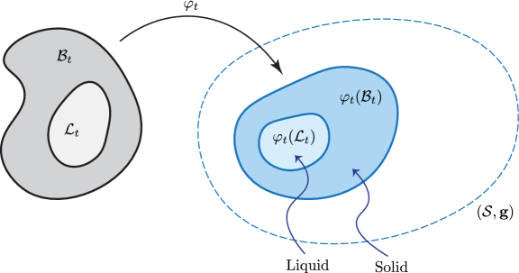
Consider a solid body with a liquid inclusion , both initially stress-free.111The effect of gravity is neglected, and hence, there is no pressure caused by the self-weight of the liquid. The initial solid-liquid body inherits a flat metric from the ambient Euclidean space. Assume that solidification (accretion) begins at . Let denote the ambient material space, which is a connected and orientable three-dimensional manifold embeddable in . Let the map assign a time of solidification (attachment) to every fluid point. The accreting solid and the ablating fluid are identified with their respective time-dependent material manifolds and (Figure 1). They are defined as follows
| (2.1) |
Note that , although . It is assumed that the differential never vanishes. Let be the accretion surface where the solidifying material is about to attach. The level sets are assumed to be manifolds, which are diffeomorphic to each other for all . This assumption ensures the existence of a material motion.
2.2 Kinematics of accretion
For an accreting body, the deformation map is assumed to be a homeomorphism for each . The deformation gradient is a two-point tensor , where and .222 Let and be local coordinate charts on and , respectively. The deformation gradient is represented as (2.2) We use the flexible notations and . Note that and form the bases for and , respectively. The material and spatial velocity fields are defined as and , respectively. Similarly, the material and spatial acceleration fields are defined as and , respectively.333 In components, and . Here, denote the Christoffel symbols for the Levi-Civita connection , i.e., . Similarly, the Christoffel symbols of are denoted as , i.e., .
The map records the placement of at its time of attachment. In general, is not injective. Moreover, the frozen deformation gradient , which captures the deformation gradient at the time of attachment, is not the tangent of an embedding, in general. Even when is an embedding, is not equal to . In fact . While is compatible within each individual layer , it is incompatible, in general. The incompatibility of the is the fundamental reason behind the existence of local anelastic distortions in accreting bodies, and hence the presence of residual stresses.
Let denote the accretion surface in the deformed configuration. The growth (accretion) velocity is a vector field that describes the velocity at which new material is being added onto , i.e., is the velocity of accreting particles relative to just before attachment. The material growth velocity, denoted as , is a vector field that characterizes the time evolution of the layers within the material ambient space. The vector field is not uniquely determined and can be selected from an equivalence class of material growth velocities that correspond to isometric material manifolds. Let and be the spatial and referential depictions of the total velocity of the accretion surface , i.e., . It can be shown that , where the term accounts for the influence of accretion.
The accretion-induced anelasticity is modeled by the accretion tensor , which is a time-independent two-point tensor, defined as
| (2.3) |
Since , it follows that . Although the accretion tensor is compatible within each individual layer, it is not the tangent map of any embedding. For more details, see (Sozio and Yavari, 2019).
Remark 2.1.
Let us consider a foliation chart induced by the time of attachment map in the ambient material manifold and a local chart in the ambient Euclidean manifold . The accretion tensor has the following representation with respect to the frames and (Sozio and Yavari, 2019)
| (2.4) |
2.3 Material metric for thermoelastic accretion
Consider a time-dependent material manifold , where the metric measures distances corresponding to the relaxed state, taking into account the thermal history of the body. In geometric thermoelasticity, the metric is a function of temperature , and is given by (Sadik and Yavari, 2017b; Sozio et al., 2020)
| (2.5) |
where is a -tensor characterizing thermal expansion properties in the solid and is a temperature independent metric.444The adjoint of deformation gradient is defined such that (2.6) where is the natural paring of -forms in with vectors in , i.e., . is a -tensor with the following coordinate representation (2.7) The volumetric coefficient of thermal expansion is given by
| (2.8) |
For a time-independent reference temperature field , it is assumed that , and hence . In the thermally accreted part of the body, is assumed to be the temperature of the attached material at its time of attachment. However, in the initial body , represents the initial temperature. The material metric for the accreted portion is calculated by pulling back the Euclidean ambient metric via the accretion tensor :
| (2.9) |
The temperature-dependent material metric is therefore given by
| (2.10) |
Let and denote the spatial and material volume elements, respectively. They are related via the Jacobian as , where
| (2.11) |
Remark 2.2.
For a thermally isotropic and homogeneous body, (2.5) is simplified as
| (2.12) |
where the scalar is related to the coefficient of thermal expansion as
| (2.13) |
The volumetric coefficient of thermal expansion in dimension three is .
Remark 2.3.
Let and denote the unit normals to and , with respect to the metrics and , respectively. The growth (accretion) velocities in the deformed and material configurations can be decomposed as follows
| (2.14) |
where . Moreover, , and (Sozio and Yavari, 2019).
3 Balance laws
3.1 Conservation of mass
Let the material and spatial mass densities be denoted by and , respectively. Let represent the material mass density corresponding to the flat metric . The mass of a sub-body is calculated as
| (3.1) |
where is the volume element corresponding to the stress-free material metric, and is related to as . The mass densities are related as and , i.e.,
| (3.2) |
The material mass continuity equation is written as
| (3.3) |
while the spatial mass continuity equation reads
| (3.4) |
Here, represents the material time derivative, while represents the partial derivative .
3.2 Stress and strain tensors
The right and left Cauchy-Green strains are defined as and , respectively.555The transpose of the deformation gradient is defined such that (3.5) In components, . Thus, and are related as . In components
| (3.6) |
Further, their inverses are denoted by and , respectively. Note that is the pull-back of the spatial metric via the deformation map (i.e. ) and is the push-forward of the material metric via (i.e. ). Moreover, and .666Here, the musical symbols ♭ and ♯ denote the flat and sharp operators that lower and raise tensor indices, respectively. In components
| (3.7) |
The principal invariants of the right Cauchy-Green strain read
| (3.8) |
Note that . The constitutive model for hyperelastic materials is given by an energy density function , per unit undeformed volume. The Cauchy stress tensor , the first Piola-Kirchhoff stress tensor , and the second Piola-Kirchhoff stress tensor are related to the energy function as
| (3.9) |
Note that and .
Remark 3.1.
Remark 3.2.
The energy function for hyperelastic fluids has the functional form , where is a smooth, strictly convex function of that diverges as approaches (Podio-Guidugli et al., 1985). Thus, the Cauchy, the first and the second Piola-Kirchhoff stress tensors are written as
| (3.11) |
Note that one must have , as hydrostatic stresses are compressive in fluids.
The energy function for homogeneous materials is independent of , i.e., for hyperelastic solids and for hyperelastic fluids.
3.3 Balance of linear and angular momenta
The localized forms of the balance of linear momentum in terms of the Cauchy and the first Piola-Kirchhoff stress read777In coordinates (3.12) where and . Note that depends on both the metrics and .
| (3.13) |
where is the spatial body force (per unit mass), while is body force referred in material coordinates, i.e., . In components
| (3.14) |
The balance of angular momentum in local form reads
| (3.15) |
Note that for slow accretion, the inertial effects can be disregarded.
Let be the spatial traction field and denote the material traction field. Consider a material surface element with unit normal , which gets mapped to the element with unit normal in the deformed configuration. The traction is related to the Cauchy stress as , and to the first Piola-Kirchhoff stress as .888Note that and . Thus, and . Note that .999The Nanson’s formula has been used here. In components, the -forms and are related as . Therefore, the force on the surface element in consideration is .
3.4 The heat equation
Let be the temperature field defined with respect to the current configuration and let be the temperature field defined with respect to the reference configuration. Since , it follows that , i.e., , or equivalently, . Recall that , and . Note that is a -form in the Euclidean ambient manifold with components , while is a -form in the material manifold with components related to via pull back, i.e., . Thus
| (3.16) |
Let denote the heat flux in the current configuration. Note that is interpreted as the flux through the surface element with unit normal . The material heat flux vector is defined via the Piola transform as
| (3.17) |
In components,
| (3.18) |
Let denote unit normal to the material surface element , which gets mapped to the deformed element . Using (3.18) and the Nanson’s formula, it is implied that , i.e., . Thus, is interpreted as the heat flux per unit undeformed area.
The generalized Fourier’s law of thermal conduction in the deformed configuration reads
| (3.19) |
where the -tensor represents the spatial thermal conductivity. In components, . The Fourier’s law in the reference configuration is written as
| (3.20) |
where denotes the material thermal conductivity. Note that the material and spatial thermal conductivity tensors are related as .101010 Using (3.18), (3.19) and (3.16), it is implied that (3.21) Hence, it can be inferred from (3.21) and (3.20)2 that . In components, . Furthermore, upon substituting (3.20)1 into the reduced form of the Clausius-Duhem inequality , it can be deduced that is a positive semi-definite tensor. The spatial heat equation reads
| (3.22) |
where is the specific heat capacity at constant strain, is the spatial thermal stress coefficient, denotes the rate of deformation tensor and represents a heat source (per unit deformed volume) term, see Appendix A. Equivalently, the material heat equation is written as
| (3.23) |
where is the material thermal stress coefficient, denotes the material rate of deformation tensor and represents a heat source (per unit undeformed volume) term, see Appendix A. The material and spatial thermal stress coefficients are related as (see Appendix A). Note that the term (or equivalently, ) can be omitted if there is no thermoelastic coupling in the material under consideration.111111A classic illustration of thermoelastic coupling is the Gough-Joule effect, observed in vulcanized rubber, where the temperature of a rubber band changes during adiabatic stretching (Gough, 1805; Joule, 1859). In the absence of heat sources, the spatial heat equation for a rigid heat conductor is written as
| (3.24) |
or, in components, . The equivalent material heat equation is written as
| (3.25) |
In components, . The heat flux in thermally isotropic solids has the following representation
| (3.26) |
where , , are scalar response functions (Truesdell and Noll, 2004). We consider the model for our numerical examples, where denotes the heat conduction coefficient.121212Note that . Further, is the traditional thermal diffusivity.
3.5 Stefan’s condition
Let and . Let and denote the heat flux per unit area on the opposite sides of the interface in the current configuration. In the absence of any phase change or heat source/sink, the jump in the normal heat flux across vanishes, i.e.,
| (3.27) |
where is the outward unit normal to .
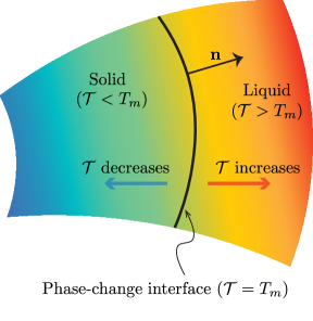
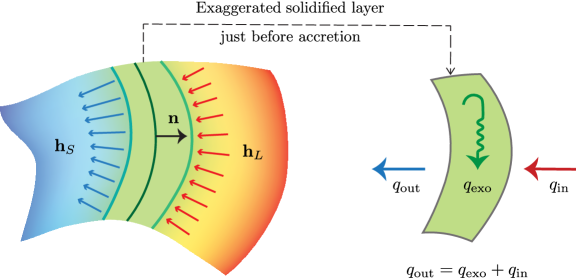
When is the solidification interface between the (cold) solid and (hot) liquid phases, it forms an isothermal surface at the melting point (Figure 2). Let be the unit normal to , pointing from solid to liquid, and let be an arbitrary subset of . Let and be the heat flux in the solid and liquid phases, respectively, in the current configuration. As one moves into the liquid phase from the solidification interface, increases, implying that points towards the solid (Figure 3). Hence, represents the rate of normal heat inflow into the subset on the interface from the liquid via conduction. There is a decrease in as one moves from the phase change interface into the solid, indicating that also points into the solid. Thus, the rate of heat flowing out normally from the subset on the interface into the solid is . The rate of mass solidified on the subset of the interface is represented by the integral (Sozio and Yavari, 2019). As solidification is exothermic, the rate of heat released in the process is expressed as , where is the specific latent heat of solidification. The heat flowing into the solid consists of two components: the heat released during solidification and the heat transferred from the surrounding liquid medium (Rubinšteĭn, 1971; Gupta, 2017). In terms of heat flow per unit time, (Figure 3), i.e.,
| (3.28) |
where is an arbitrary subset. The localized Stefan’s condition therefore reads
| (3.29) |
where represents the mass accreted, per unit area, per unit time. The localized Stefan’s condition in the reference configuration is expressed as
| (3.30) |
Note that if the liquid is initially at the solidification temperature, there is no heat flux in the liquid phase, i.e., . In this case, Stefan’s condition is simplified as
| (3.31) |
Thus, the heat entering the solid from the phase change interface is equal to the heat generated in the process of solidification.
4 Radially inward solidification in a cold rigid container
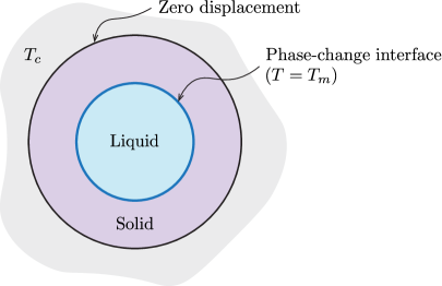
Consider a spherical container of radius , filled with a liquid initially at uniform temperature . The inner wall of the container is maintained at a constant temperature . Let denote the melting point of the material, satisfying the condition . At , the outermost layer of liquid begins to cool down and solidifies when the melting point is reached. The container wall acts as a rigid substrate to which the outermost accreted layer firmly attaches, resulting in no displacement of the outer boundary of the accreting body. Layers of liquid solidify and attach to the inner surface of the accreting body—a spherical shell, causing the solidification front to progress inward (Figure 4). The temperature fields within the accreting body and the liquid are both unknowns.131313This problem draws inspiration from the experiments conducted by Chan and Tan (2006) who investigated the inward solidification of an hexadecane in a spherical enclosure (capsule) with walls maintained at a constant temperature. They placed this capsule in a cool water tank that was consistently stirred and supplied with cold water from a refrigerated bath. They attached thermocouples to the capsule walls to track its temperature and ensure that it remains constant throughout the process.
We model both the liquid and solid phases as isotropic compressible hyperelastic materials. To simplify the analysis, an assumption can be made that , allowing for solidification to initiate near the container wall at (Stewartson and Waechter, 1976; Rabin and Steif, 1998).
4.1 Kinematics
The ambient space has the Euclidean metric
| (4.1) |
in terms of the spherical coordinates , where , and .
Let denote the material radius corresponding to the inner surface of the solid at any time , where is the time taken for the completion of freezing. Note that is assumed to be a continuous bijective map on with the initial condition . The inverse map assigns the time of attachment to each spherical layer in the material manifold. The accreting solid and the ablating fluid are identified with the following time-dependent material manifolds
| (4.2) | ||||
Let the temperature field be denoted as , and defined piece-wise as follows
| (4.3) |
Note that is continuous at the solidification interface (Caffarelli and Evans, 1983), i.e., . The material metric for the liquid phase in its initial state reads
| (4.4) |
where are the material spherical coordinates. Thus, the temperature-dependent material metric for the liquid phase is written as
| (4.5) |
where the scalar function characterizes isotropic and homogeneous thermal expansion in the liquid phase. We consider radial deformations , where and , and
| (4.6) |
and , .141414Podio-Guidugli et al. (1985) investigated cavitation in hyperelastic fluids undergoing similar radial deformations. They termed the deformations satisfying the condition regular, and those with , irregular deformations corresponding to a cavity (hole) of radius . Note that is continuous at for all . Let and . Thus, , or .151515Note that (4.7) and thus (4.8) Hence, the velocity field is continuous at if and only if the partial derivative is also continuous at . The moving phase-change interface in the reference and current configurations are represented as
| (4.9) | ||||
The respective deformation gradients in the solid and liquid phases read
| (4.10) |
Let be the material accretion velocity. Let denote the growth velocity in the current configuration, i.e., is the relative velocity of the accreting particles with respect to the interface . Further define and . Thus, the accretion tensor has the following representation with respect to the frames and :161616In our example, and . Recall that the components of the accretion tensor are defined as (4.11) Further, . Thus, the nonzero components of are (4.12)
| (4.13) |
The accreting layer is not stress free due to the pressure exerted by the fluid. Let be the natural metric of the pre-stressed layers that are accreting to the solid. This metric is obtained by transforming the Euclidean metric via a pre-deformation tensor as . In this case, the material metric for the accreted layer is calculated by pulling back the natural metric via the accretion tensor (Sozio and Yavari, 2019). Therefore, one has
| (4.14) |
In this example, it is assumed that
| (4.15) |
where the function represents radial dilation if and radial contraction if . Thus, the temperature-independent material metric at the time of accretion is written as
| (4.16) |
where . Thus, the temperature-dependent material metric for the solid phase is written as
| (4.17) |
where the scalar function characterizes isotropic and homogeneous thermal expansion in the solid phase. The Jacobian of the deformation is written as
| (4.18) |
Further, and are the coefficients of thermal expansion in the solid and liquid phases, respectively.
4.2 Balance laws
4.2.1 Conservation of mass
The mass of the liquid and solid portions are calculated as171717 Alternatively, one has , and .
| (4.19) | ||||
Thus, the total mass of the system is written as
| (4.20) |
Using the Leibniz rule, it can be shown that
| (4.21) |
As the mass of the entire body is conserved, . Since is nonzero, it follows from (4.21) that
| (4.22) |
The material continuity in the respective phases read181818Note that (4.23) where the relations and have been used. Therefore, (4.24) follows from (3.3) and (4.23).
| (4.24) | |||
The density is assumed to be a function of temperature, i.e., and . It follows that and , where and are the reference temperatures for the solid and liquid phases, respectively. Thus, the respective continuity equations in (4.24) are rewritten as
| (4.25) |
This is integrated to obtain
| (4.26) |
which are equivalent to
| (4.27) |
Note that is the initial temperature of the liquid, while represents the accretion temperature, i.e., .
Remark 4.1.
To simplify the problem, it can be assumed that the liquid is initially at the solidification temperature, i.e., . Thus, there is no heat transfer in the liquid medium, i.e., . Thus, it follows from (4.27)2 that , which is a constant for homogeneous fluids.191919Alternatively, by substituting into (4.24)2, it is implied that . Similarly, , where is a constant for homogeneous solids. As , it follows from (4.24)2 that . Therefore, one has
| (4.28) |
Thus
| (4.29) |
Further, the mass fraction solidified up to time is simplified as .
Remark 4.2.
The Jacobian is rewritten as
| (4.30) |
4.2.2 Heat equation
Let denote the spatial heat flux in material coordinates, i.e., , with being the material heat flux. In the model , the radial components of and within the solid are as follows
| (4.31) |
Note that202020Here, we have used the fact that (4.32) In spherical coordinates, one has (4.33) The Christoffel symbols for the material metric are given in (C.3).
| (4.34) |
where the notation has been used. Therefore, the heat equation (3.25) inside the solid is written as
| (4.35) |
Let us assume that the heat conduction coefficient is independent of temperature, i.e., , a constant. Thus, using (4.28), the heat equation (4.35) is simplified as follows
| (4.36) |
where the constant is analogous to thermal diffusivity. Further, the temperature field satisfies the following boundary conditions
| (4.37) | ||||
where is the coefficient of heat transfer between the walls of the container and the solidified material. Thus, for the temperature field, we have a Neumann boundary condition near the fixed wall of the container and a Dirichlet boundary condition on the moving interface.
4.2.3 Stefan’s condition
The rate of mass transferred from liquid to solid phase is . The rate of mass solidified is
| (4.38) |
Alternatively, can be expressed as
| (4.39) |
The time rate of heat released during solidification is . Further, the heat transferred into the solid medium is
| (4.40) |
If the liquid is initially at the solidification temperature, there is no heat flux within it, and the heat entering the solid from the phase change interface is equal to the heat generated during solidification. Thus, Stefan’s condition is written as
| (4.41) |
or equivalently,
| (4.42) |
Assuming a constant heat conduction coefficient , Stefan’s condition is written as
| (4.43) |
where .
4.2.4 Conservation of linear momentum in the solid portion
The Cauchy stress tensor in the solid portion is related to the energy function as follows212121Note that the first Piola-Kirchhoff stress tensor is written as (4.44) where and .
| (4.45) |
Since , , one has , and .222222The Christoffel symbols for the Euclidean metric are given in (C.1). Using (3.12) and (C.1), the radial equilibrium equation (3.13) is simplified to read
| (4.46) |
The inertial effects can be ignored if the solidification process is slow, and hence in the absence of body forces, it follows from (4.46) that
| (4.47) |
In this example,232323Recall that the components of and are related as . Thus, the components are .
| (4.48) |
Further, the principal invariants of read242424Here, we have used the fact that (4.49)
| (4.50) | ||||
The Cauchy stress has the following nonzero components
| (4.51) | ||||
Substituting (4.51) in (4.47), one obtains252525The relation has been used here.
| (4.52) |
In the solid, one has . Thus, (4.52) is simplified as
| (4.53) |
where for . Using (4.28), (4.53) is rewritten as follows
| (4.54) |
Hence, (4.54) can be integrated to obtain
| (4.55) | ||||
Remark 4.3.
Note that has to be continuous at in order to satisfy the traction continuity across the phase change interface.
4.2.5 Conservation of linear momentum inside the liquid
The Cauchy stress inside the liquid is related to the energy function as , i.e.,
| (4.56) |
Note that . In the absence of inertial effects and body forces, the radial equilibrium equation is written as
| (4.57) |
Hence, it follows that , i.e., is independent of . Moreover, one has
| (4.58) |
If the liquid is initially at the melting temperature, then and there is no heat transfer occurring inside the liquid during the entire process. Because there are no temperature changes, and, consequently, remain independent of temperature. Let us define the temperature-independent function as , and denote . Since , it follows from (4.58) that (Podio-Guidugli et al., 1985). Thus, is independent of , which is indicated as , for some function . Note that because throughout the process. Since (4.30)1 is simplified as , it is implied that inside the liquid one has
| (4.59) |
Since , it follows from (4.59) that , and hence .262626Furthermore, it is implied that and inside the liquid. Thus, and , which agrees with the fact that . Thus,
| (4.60) |
In our numerical examples, we consider the following temperature-independent energy function
| (4.61) |
where denotes the the bulk modulus of the liquid at temperature , while represents the initial pressure in the liquid (Ghosh and Lopez-Pamies, 2022). Hence, , and . If the liquid is initially stress-free, i.e., , then, it can be deduced from that . Therefore, one has
| (4.62) |
This means that the Cauchy stress remains uniform in a compressible hyperelastic fluid in the absence of inertial effects, body forces, and heat flow.
4.3 Stefan’s problem for a neo-Hookean solid
Consider the following energy function for a thermoelastic neo-Hookean solid (Sozio et al., 2020)
| (4.63) |
where and . For more details, refer to Appendix B. The nonzero components of Cauchy stress read
| (4.64) |
where . These coefficients are calculated as follows
| (4.65) |
Further, we assume that depends on the temperature as per the following relation (see (B.4))
| (4.66) |
Since is continuous across , it follows from (4.55) and (4.62) that
| (4.67) |
Thus, using (4.64)1 and (4.28), (4.67) is rewritten as
| (4.68) | |||
where
| (4.69) | ||||
Therefore, for the neo-Hookean solid, the moving boundary problem on the domain is written as272727Recall that (4.70)1 was obtained in (4.68), while (4.70)2 restates the heat equation (4.36), and (4.70)3 is Stefan’s condition (4.43). The thermal boundary conditions are written in (4.70)4 and (4.70)6, while (4.70)5 and (4.70)7 are the kinematic boundary conditions. Finally, (4.70)8 denotes the initial condition for the position of the moving interface.
| (4.70) |
where the temperature field , the radial placement map , and the location of the moving boundary are unknown.
Remark 4.4.
Non-dimensionalization.
| Category | Definitions |
|---|---|
| Independent variables | |
| Dependent unknown variables | |
| Dimensionless constant parameters | |
Let and be the dimensionless radial coordinate and time variable, respectively. The dimensionless radial placement map, temperature field and the location of phase-change interface are denoted by , and , respectively. These dimensionless quantities are defined in Table 1. It follows from (4.70)1 and (4.69) that for :282828Since and , it follows from (4.66) that and .
| (4.74) | ||||
where , and , , , , are dimensionless constant parameters defined in Table 1.292929 The non-dimensionalized traction continuity condition across the moving interface reads (4.75)
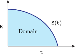
Similarly, for , the heat equation (4.70)2 is rewritten as
| (4.76) |
and, (4.70)3-8 are rewritten as
| (4.77) | ||||
where , are dimensionless constant parameters defined in Table 1. Thus, (4.74)-(4.77) constitute the non-dimensionalized boundary-value problem on the evolving domain (Figure 5).303030Recall that represents the mass fraction solidified. Further, the physical components of the Cauchy stress in the solid are non-dimensionalized as (no summation).313131Note that . Similarly, the pressure in the liquid, which is independent of , is non-dimensionalized as .323232It is implied from (4.62) that .
Remark 4.5.
Note that (4.76) is rewritten as
| (4.78) |
which is integrated using (4.77)1-6 to obtain
| (4.79) |
Since333333This is implied from the fact that .
| (4.80) |
it follows from (4.79) that343434Note that the change of variable has been used here.
| (4.81) |
Thus, Stefan’s condition (4.77)1 can be replaced with the integral constraint (4.81).
Remark 4.6.
Let be the time when the layer with radial coordinate solidifies and attaches to the shell, i.e., . Let and denote the radial placement and temperature fields, respectively, expressed as functions of and , i.e.,
| (4.82) |
Thus, the heat equation (4.76) is rewritten in terms of and as353535The following relations have been used here (4.83) where . These are obtained by differentiating the definition (4.82) with respect to .
| (4.84) | ||||
where , and thus . Note that (4.84) can be rearranged as follows
| (4.85) |
Similarly, (4.74) is rewritten as
| (4.86) | ||||
and, (4.77) is rewritten as
| (4.87) | ||||
Hence, the transformed system of equations (4.85)-(4.87) form a boundary-value problem over the fixed triangular domain , where is the time taken for complete solidification, i.e., .
Remark 4.7.
For , consider the ratio . Let and denote the radial placement and temperature fields, respectively, expressed as functions of and , i.e.,
| (4.88) |
This change of variable transforms the triangular domain into the rectangular domain . Further, the derivatives of and are related to those of and as
| (4.89) |
and,
| (4.90) |
where . Note that the thermal and displacement boundary conditions in (4.87) are expressed in terms and as follows
| (4.91) | ||||
Thus, it follows from (4.91)3 that . Therefore, (4.84) is rewritten in terms of and as
| (4.92) | ||||
Similarly, (4.86) is rewritten as
| (4.93) | ||||
Hence, (4.92), (4.93) and (4.91) form a system of nonlinear PDEs coupled with an ODE,363636Note that the integral equation (4.93) can be differentiated with respect to to get rid of the integral term. Thus, (4.93) and (4.92) are second-order nonlinear PDEs in terms of the unknown fields and . Similarly, (4.91)1 is an ODE in terms of the unknown function . with the unknown fields , , and over the rectangular domain .
Remark 4.8.
Note that the standard heat equation is recovered by setting and in (4.36), which is written as
| (4.94) |
Therefore, in the absence of any elastic deformation or thermal expansion, the non-dimensionalized moving boundary problem reads
| (4.95) | ||||
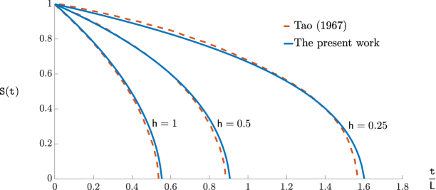
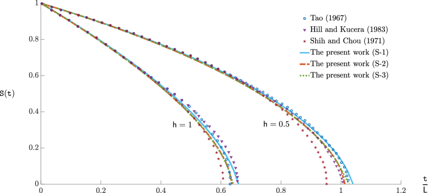
where and . Here, is the Biot number, and is the Stefan number. The phase change problem (4.95) has been analyzed by London and Seban (1943), Tao (1967), Shih and Chou (1971), Hill and Kucera (1983), and possibly others. Furthermore, (4.81) is simplified as
| (4.96) |
Alternatively, since (4.95)1 is rewritten as , it can be shown using (4.95)2-5 that Stefan’s condition (4.95)2 is equivalent to373737Using (4.95)2-4, it is implied that (4.97) Therefore, since , (4.99) follows from (4.95)5 and the fact that (4.98)
| (4.99) |
Thus, for a rigid conductor, Stefan’s condition (4.95)2 can be replaced with the integral constraint (4.96), or equivalently with (4.99).
4.4 Residual stresses
The solidification process is stopped at time , when the the solid-liquid interface is at in the reference configuration, or equivalently at in the current configuration. Imagine that the accreted solid is drained of the remaining liquid and is allowed to reach a steady-state uniform temperature of in an ambient environment, while its inner and outer boundaries are traction-free. The resulting residually-stressed configuration is denoted by . The material metric for the solid is written as
| (4.100) |
Recall that
| (4.101) |
Note that since is now a known function defined on the interval , determined from the solution of the IBVP during accretion, the material metric is considered to be given.
Let denote the deformation map corresponding to the residually-stressed configuration. In spherical coordinates , where the placement map represents the residual radial distortion. The deformation gradient reads
| (4.102) |
The Jacobian of the deformation is written as
| (4.103) |
The strain tensors for this configuration are given as
| (4.104) |
Further, the principal invariants of read
| (4.105) |
Example 4.9 (A neo-Hookean solid).
The thermoelastic neo-Hookean solid considered in (4.63) is now at a constant temperature, and thus, is characterized by the temperature-independent energy function
| (4.106) |
The nonzero components of residual Cauchy stress are written as
| (4.107) |
where the coefficients and are given as
| (4.108) |
The balance of linear momentum in the absence of body forces and inertial effects is simplified to yield the following radial equilibrium equation
| (4.109) |
Furthermore, the outer and inner boundaries are traction-free, i.e.
| (4.110) |
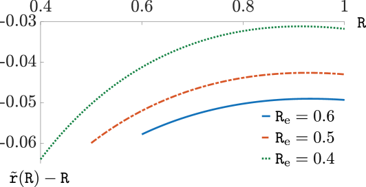
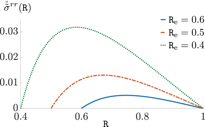
It follows from (4.107), (4.108) and (4.105)1 that (4.109) is a nonlinear ODE in terms of , with the boundary conditions (4.110). Thus, the problem of finding the residual stresses and distortions boils down to solving the boundary-value problem (4.109)-(4.110) for the unknown function . This problem is then non-dimensionalized according to Table 1. The dimensionless radial displacement and the dimensionless physical components of the Cauchy stress (no summation) in the residually-stressed configuration at a given dimensionless steady state temperature are illustrated in Figure 14.383838Note that and .
4.5 Numerical results and discussion
Several numerical methods for the solution of moving boundary value problems have been proposed over the years (Rubinšteĭn, 1971; Crank, 1984). In this work, we follow the approach of Douglas and Gallie (1955), where for a specified space grid, the corresponding instances of time are calculated as the moving boundary assumes these discrete positions in progression. It should be noted that the bijectivity of is exploited here, allowing us to treat the time of accretion as the unknown. For each unknown time step, the moving interface is first assigned a position. Treating the domain as fixed, we calculate the deformation and temperature fields, along with the instant of time for this interface location, by solving the conservation of linear momentum, transient heat equation, and Stefan’s condition. This is implemented using a finite difference approximation (an implicit scheme) in Matlab. The optimum time step that minimizes the residue from Stefan’s condition to ensure a sufficiently small magnitude is calculated using fminunc, while the corresponding numerical solution for the radial equilibrium and the heat equation is simultaneously obtained using fsolve. Extensive parametric studies are conducted by varying the numerical values of the dimensionless constants in Table 1. The observations from the numerical results are qualitatively described in the following.
-
•
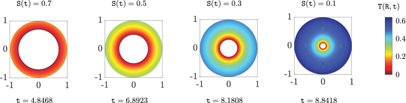
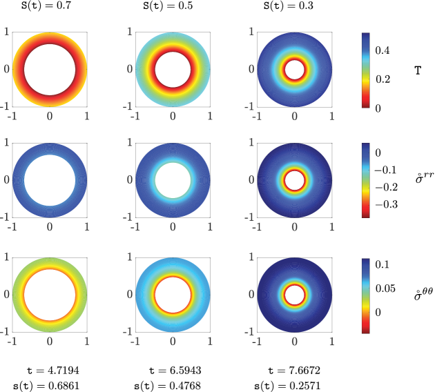
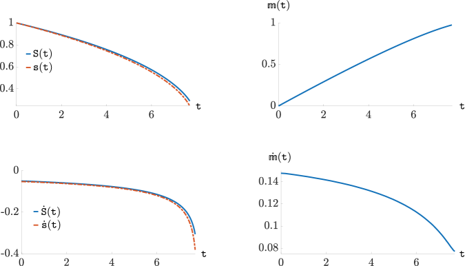
The radial speed of the interface, in both the reference and the current configurations, is observed to increase as the interface moves inward with time (Figure 10). As expected, the fraction of the initial liquid mass solidified increases over time. However, the rate of mass fraction solidified decreases with time (Figure 10). These trends are similar to what has been observed in the rigid conductor case (see Figures 6 and 7). The temperature field inside a rigid conductor is shown at different instances of time in Figure 8. It should be noted that most numerical studies in the literature for the rigid conductor case only depict the motion of the interface (Tao, 1967; Shih and Chou, 1971; Hill and Kucera, 1983). The experimental studies report the rate of solidification with the rate of change of mass fraction of the total initial liquid solidified with respect to time (Chan and Tan, 2006). This is possibly because the liquid inclusion tends to lose its spherical shape and concentricity with the previously accreted layers as the inclusion size decreases. The trend we observe for the variation of mass fraction solidified qualitatively agrees with that of Chan and Tan (2006), although a direct comparison with the experimental data is not feasible due to the unavailability of a complete set of material properties of the substances used. The temperature field and the physical components of the Cauchy stress in the deformed solid for the coupled problem (4.74)-(4.77) are depicted in Figure 9.
-
•
The symbol denotes the ratio of the density of the undeformed solid to that of the liquid near the melting point. Solidification of a given mass of a liquid with results in a reduction of the occupied volume. As the accretion surface moves inward, layers of liquid are replaced with denser solid layers, leading to a decrease in volume. Furthermore, since the container has fixed walls and, therefore, a fixed volume, the liquid inclusion naturally develops positive hydrostatic stress as soon as solidification begins, indicating possibility of cavitation. Although this is confirmed numerically, the observed data is excluded from figures as positive liquid pressure is not physically possible. Moreover, it follows from that a negative liquid pressure is equivalent to a negative radial displacement of the accreting layers (see Figures 11(b) and 11(a)).393939Since is the position of the solidification interface in the deformed configuration, and was its position in the initial liquid pool, , or equivalently, , denotes the radial displacement of an accreting layer. As the solidification interface approaches the center, the magnitude of the displacement of the accreting layers increases rapidly, requiring it to decelerate and decrease swiftly to ultimately vanish at the center.404040The time instant marking the completion of solidification must satisfy . Further, if this is achieved without cavitation, then . Thus, . Thus, the mesh near the center must be much finer; otherwise, numerical techniques that better accommodate such sudden fluctuations need to be employed.
-
•
The figures shown in this section are based on the assumption . With this assumption, an accreting layer with a given mass tends to occupy a greater volume upon solidification, compressing the liquid inclusion and resulting in negative hydrostatic stress. The magnitude of this negative hydrostatic stress increases with time as the solidification interface moves inward (Figure 13). The extra volume occupied by the solidifying layers piles up to create a significant gap, causing the pressure in the liquid to become highly compressive as the interface approaches the center.
-
•
Surface stresses play a significant role for liquid inclusions smaller than a certain limit determined by the elastocapillarity length—the ratio of surface tension to the bulk modulus (Bico et al., 2018). In this paper we do not consider surface stress, and hence, do not report the numerical results for very small liquid inclusions. Although the process is halted a while before complete solidification, the rate of increase in the magnitude of liquid pressure is significantly high by the time this margin is reached.
-
•
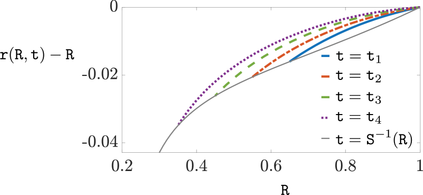
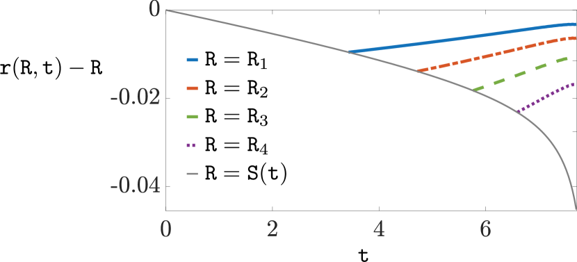
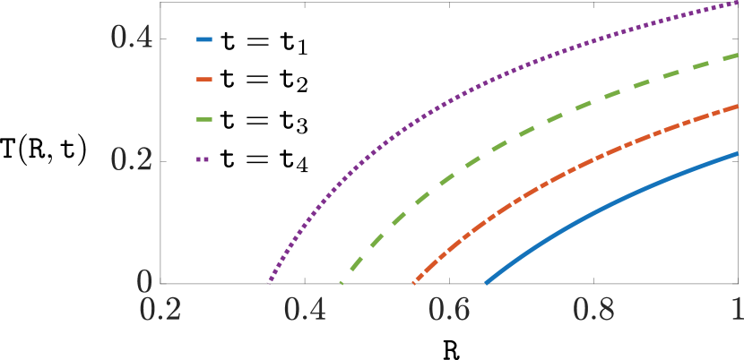
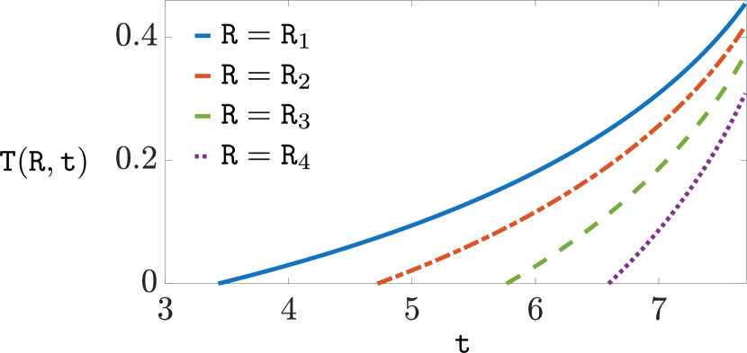
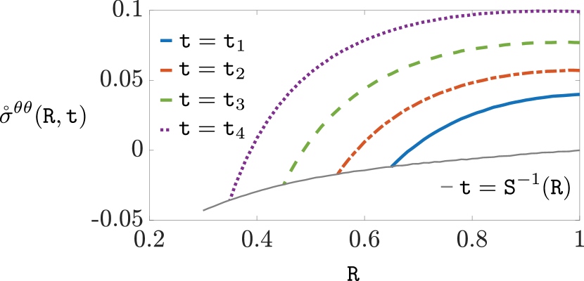
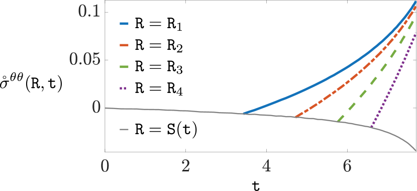
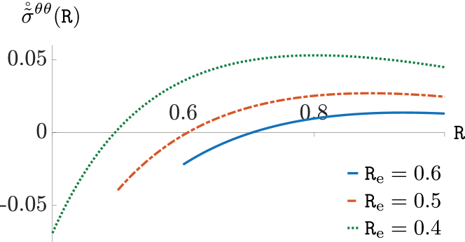
Note that at the melting point, and since , increases as the real temperature decreases (see Figures 8 and 9). The moving interface is always at the melting point, and the temperature decreases as one moves towards the fixed wall (Figure 11(c)). The temperature at a point decreases over time after it is accreted (Figure 11(d)). Radial displacements are always negative, and the magnitude at any accreted point decreases over time (Figure 11(b)). At any instant, the magnitude of radial displacement is maximum at the moving boundary and decreases to zero at the fixed boundary (Figure 11(a)).
-
•
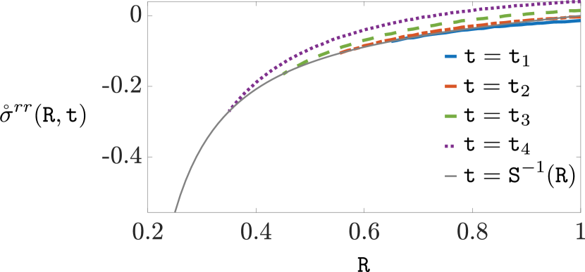
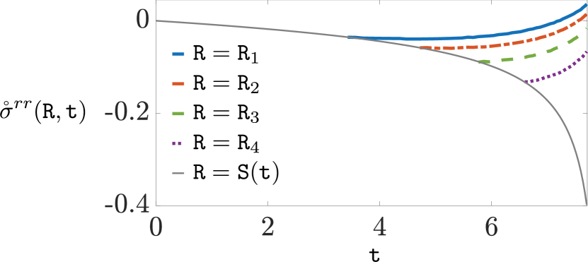
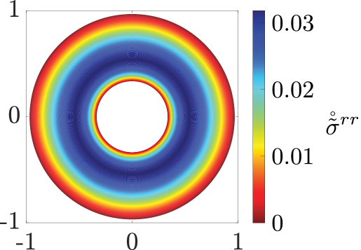
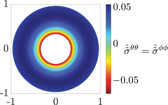
Both and are negative near the moving boundary. increases as one moves away from the inclusion (i.e., decreases in magnitude), vanishes somewhere in between, and eventually becomes positive near the wall (Figure 11(g)). decreases in magnitude as one moves away from the inclusion but remains negative if the inclusion size is too large (Figure 11(e)). However, when the interface has moved far enough from the wall, can be positive near the wall, decreasing to a negative value near the inclusion. At any accreted point, is initially negative and decreases in magnitude over time (Figure 11(f)). For points closer to the fixed wall, eventually becomes positive as the inclusion size decreases. is initially negative for all accreted points, and quickly transitions to a positive value, except for the points accreted just before the process is halted (Figure 11(h)).
-
•
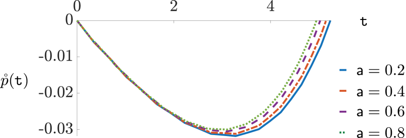
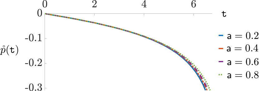
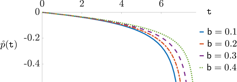
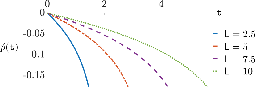
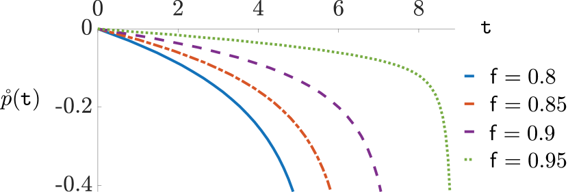
The dimensionless parameter describes the thermal expansion properties of the solid relative to the temperature difference between its melting point and the cold wall temperature. A larger implies a higher contraction of the solid for a given temperature drop. It is observed that the rate of increase in liquid pressure magnitude is much faster for lower values of (Figure 13(d)). If is too large, the liquid inclusion pressure decreases from zero until it reaches a minimum, and then increases until it becomes zero again (Figure 13(b)). Positive pressure solutions beyond this point are physically meaningless due to the possibility of cavitation and are therefore discarded. The reason behind this tendency of liquid cavitation, even with , is the extremely high thermal contraction in the colder layers closer to the container walls. represents the ratio of the temperature difference between the cold container wall and the melting point of the liquid to the absolute melting temperature. Figures 13(a) and 13(c) describe the influence of on the evolution of the liquid pressure within the inclusion for the two distinct categories of discussed above.
-
•
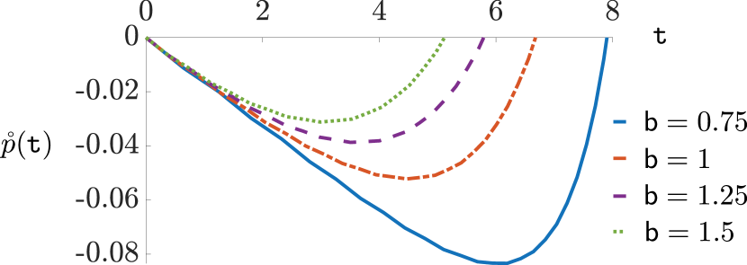
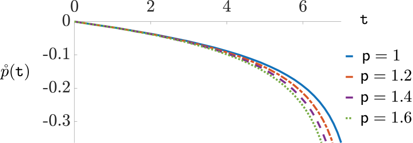
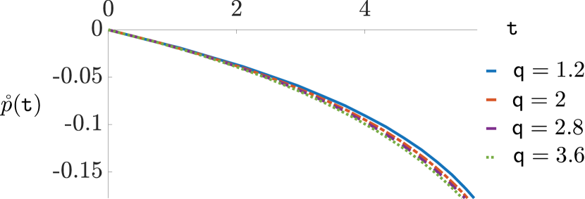
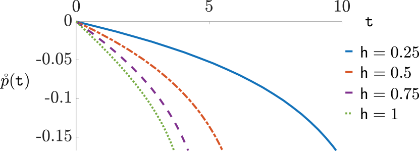
The elastic material properties are captured by and , which represent the shear and bulk modulus, respectively, of the solid near the melting point as compared to the liquid bulk modulus near the solidification temperature. The magnitude of pressure in the liquid inclusion rises faster with larger and values (see Figures 13(e) and 13(f)). The specific latent heat of solidification appears only in the dimensionless constant , which is loosely interpreted as a measure of the latent heat released relative to the heat capacity of the solid. The heat transfer with the container walls is incorporated in the coefficient , loosely quantifying how much of the heat conducted towards the outer boundary of the accreted solid is transferred out into the cold wall.
-
•
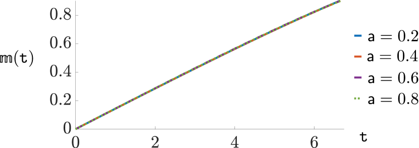
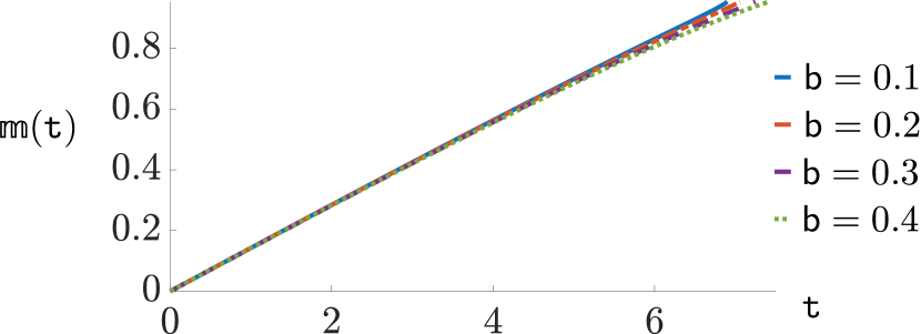
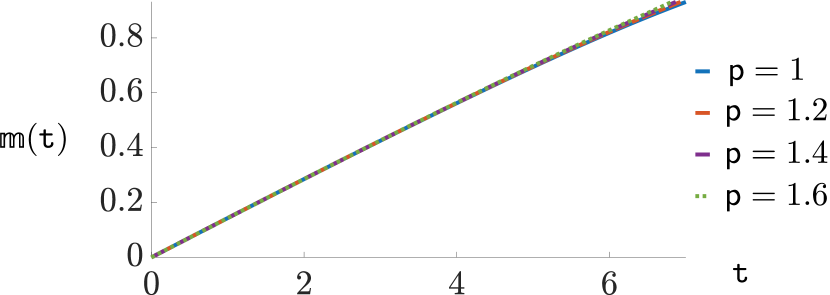
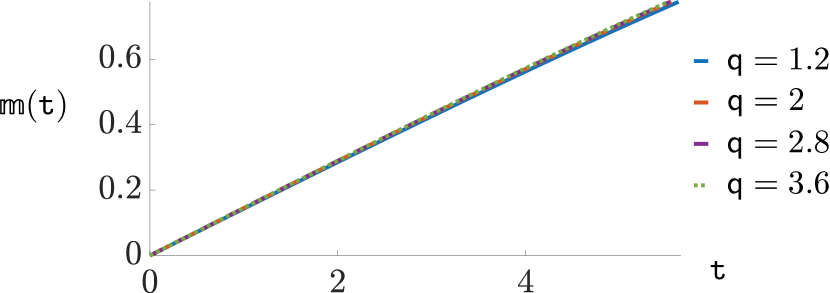
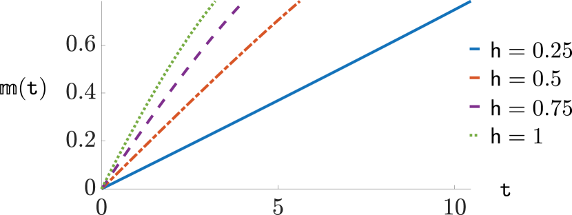
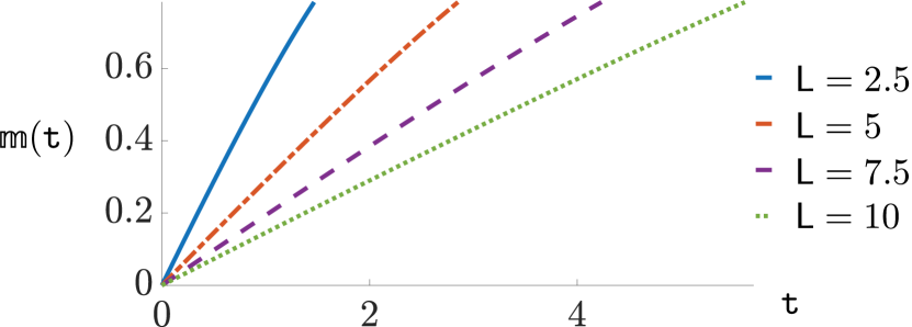
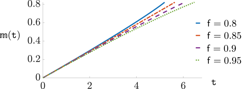
The numerical variations in , , , and used for the parametric studies do not significantly impact the solidification rate, indicating a lower sensitivity to these parameters (see Figures 12(a), 12(b), 12(c) and12(d)). A value of closer to , with the liquid denser than the solid near melting, results in slower solidification (Figure 12(g)); and the sensitivity to variations in is moderate. The solidification rate is highly sensitive to and . A larger implies that the heat is able to flow more efficiently out of the solid into the container walls, facilitating in faster solidification (Figure 12(e)). A smaller implies less specific latent heat compared to the specific heat capacity, allowing the accreted solid to better absorb the heat released during solidification. This indirectly promotes outward heat conduction and results in a higher solidification rate (Figure 12(f)). The higher rates of pressure drop in the liquid for larger and smaller values (see Figures 13(g) and 13(h)) are attributed to the faster solidification rates.
-
•
The configuration obtained by detaching the accreted solid from the rigid walls of the cold container after a given time, removing any remaining unsolidified liquid, and subsequently cooling the solid to a uniform steady-state temperature is not stress-free (see Figures 14(d) and 14(e)). In this configuration, both the inner and outer boundaries are displaced inward relative to their positions in the initial liquid (Figure 14(a)). The inward displacement of the outer boundary is likely caused by thermal contraction. The inner layers experience highly negative during accretion, owing to the presence of a pressurized liquid inclusion. When the liquid is removed and the inner boundary becomes traction-free, the inner layers naturally tend to move apart to relieve the negative stress. Moreover, the closer the layer is to the inner boundary, the more pronounced this tendency becomes. In the residually-stressed configuration, is zero at the inner boundary, increases as one moves outward, reaches a maximum, and then decreases to vanish at the outer boundary (Figure 14(d)). The maximum value of is larger if the accretion process ends later (Figure 14(b)). is negative at the inner boundary, increases as one moves outwards, eventually becoming positive at the outer boundary (Figure 14(e)). The variation in is larger if the solidification process is stopped later (Figure 14(c)). Consequently, the outer boundary is prone to developing cracks, while the inner boundary is prone to buckling instabilities.
5 Conclusions
In this paper, the process of liquid-to-solid phase change was modeled as a thermoelastic accretion problem. Several simplifying assumptions were made, such as neglecting inertial effects in both phases, assuming the melting temperature to be independent of pressure (hydrostatic stress in the liquid), ignoring surface stresses, and assuming that the thermal conductivity and heat capacity of the solid are temperature-independent. Since the primary focus was on studying the solidification of a liquid inclusion, the liquid was assumed to be a compressible hyperelastic material, allowing deformation. The problem of determining the reference configuration as the solid portion of a deformable body grows by accretion has the following challenging aspects: first, determining the set of material points that are part of the solid (i.e., knowledge of the boundary location); second, determining the material metric at each point. The material metric depends on the state of deformation of the solidifying material during attachment and on the temperature evolution to account for the effects of thermal expansion. The boundary location, or the set of material points included in the solid at a given instant of time, is determined by the mass rate of solidification, which depends on the jump of the heat flux across the moving interface. Thus, this is a coupled nonlinear problem where the location of the boundary is an unknown, in addition to the deformation and temperature fields.
As a concrete example, the radially inward solidification of a liquid initially at the melting temperature was studied. The resulting moving boundary problem was numerically solved by treating the time of attachment map as an unknown, instead of the boundary location. In other words, for a given space grid, the time instances when the moving boundary crosses these grid points were calculated. This formulation enables one to study the deformation and stresses at any point inside the solid at any desired time, thus potentially highlighting critical zones prone to failures and instabilities. However, the solidification process is halted with a margin prior to completion due to multiple reasons. The numerical results become less accurate as one approaches the center, and they are also physically irrelevant as surface stresses, which become dominant for smaller inclusion sizes, are not considered in the formulation. A detailed parametric study was performed by varying all the dimensionless constants. In all the numerical examples, the solid was assumed to be less dense than the liquid near the melting point, commonly observed in water and some polymers, though rare in metals. This assumption is essential to avoid cavitation inside the liquid in the context of a solidifying inclusion. However, even with this assumption of denser liquids, our numerical results show that cavitation might be possible in the case of extreme thermal contraction in the solid. The accreted body—once it is detached from the rigid container, drained of the remaining unsolidified liquid, and cooled to an ambient temperature—is residually-stressed, in general. The residually-stressed configuration and its residual stresses were computed numerically.
The present study opens up several new avenues for future investigations. The zero-displacement boundary condition imposes a volumetric constraint, potentially causing cavitation for materials denser in the solid phase near the melting point. This results from volume changes due to jump in density across phases. Replacing it with, for instance, an applied pressure on the outer boundary may enable one to study solidification across a broader range of materials. Developing a variational theory to study instabilities in both solids and liquids during a solidification process is another extension. It is crucial to include surface stresses in the theory for a more realistic understanding of the physics and mechanics of solidification in simple, computationally feasible problems. Ultimately, a more general computational framework needs to be developed to fully utilize the benefits of this formulation for more complex geometries in real-world applications.
Acknowledgement
We benefited from discussions with Aditya Kumar and Souhayl Sadik. This work was supported by NSF – Grant No. CMMI 1939901.
References
- Abeyaratne and Knowles [1993] R. Abeyaratne and J. K. Knowles. A continuum model of a thermoelastic solid capable of undergoing phase transitions. Journal of the Mechanics and Physics of Solids, 41(3):541–571, 1993.
- Abeyaratne et al. [2022a] R. Abeyaratne, E. Puntel, F. Recrosi, and G. Tomassetti. Surface accretion of a pre-stretched half-space: Biot’s problem revisited. Journal of the Mechanics and Physics of Solids, 167:104958, 2022a.
- Abeyaratne et al. [2022b] R. Abeyaratne, E. Puntel, and G. Tomassetti. On the stability of surface growth: The effect of a compliant surrounding medium. Journal of Elasticity, pages 1–25, 2022b.
- Ateshian and Shim [2022] G. A. Ateshian and J. J. Shim. Continuum thermodynamics of the phase transformation of thermoelastic fluids. arXiv preprint arXiv:2207.14158, 2022.
- Bachmann et al. [2021] J. Bachmann, P. Obst, L. Knorr, S. Schmölzer, G. Fruhmann, G. Witt, T. Osswald, K. Wudy, and O. Hinrichsen. Cavity vat photopolymerisation for additive manufacturing of polymer-composite 3d objects. Communications Materials, 2(1):107, 2021.
- Bažant et al. [1997] Z. P. Bažant, A. B. Hauggaard, S. Baweja, and F.-J. Ulm. Microprestress-solidification theory for concrete creep. i: Aging and drying effects. Journal of Engineering Mechanics, 123(11):1188–1194, 1997.
- Bico et al. [2018] J. Bico, É. Reyssat, and B. Roman. Elastocapillarity: When surface tension deforms elastic solids. Annual Review of Fluid Mechanics, 50:629–659, 2018.
- Binder [1987] K. Binder. Theory of first-order phase transitions. Reports on Progress in Physics, 50(7):783, 1987.
- Budak et al. [1965] B. Budak, F. Vasil’ev, and A. Uspenskii. Difference methods for solving certain boundary value problems of stefan type. Chislennye metody v gazovoi dinamike, pages 139–183, 1965.
- Buffett et al. [1992] B. A. Buffett, H. E. Huppert, J. R. Lister, and A. W. Woods. Analytical model for solidification of the earth’s core. Nature, 356(6367):329–331, 1992.
- Buffett et al. [1993] B. A. Buffett, P. Mathews, T. Herring, and I. Shapiro. Forced nutations of the earth: contributions prom the effects of ellipticity and rotation on the elastic deformations. Journal of Geophysical Research: Solid Earth, 98(B12):21659–21676, 1993.
- Buffett et al. [1996] B. A. Buffett, H. E. Huppert, J. R. Lister, and A. W. Woods. On the thermal evolution of the earth’s core. Journal of Geophysical Research: Solid Earth, 101(B4):7989–8006, 1996.
- Caffarelli and Evans [1983] L. A. Caffarelli and L. C. Evans. Continuity of the temperature in the two-phase stefan problem. Archive for Rational Mechanics and Analysis, 81(3):199–220, 1983.
- Carslaw and Jaeger [1959] H. Carslaw and J. Jaeger. Conduction of Heat in Solids. Clarendon Press, Oxford, 1959.
- Chambre [1956] P. Chambre. On the dynamics of phase growth. The Quarterly Journal of Mechanics and Applied Mathematics, 9(2):224–233, 1956.
- Chan and Tan [2006] C. Chan and F. Tan. Solidification inside a sphere—An experimental study. International Communications in Heat and Mass Transfer, 33(3):335–341, 2006.
- Coussy [2005] O. Coussy. Poromechanics of freezing materials. Journal of the Mechanics and Physics of Solids, 53(8):1689–1718, 2005.
- Crank [1984] J. Crank. Free and Moving Boundary Problems. Oxford University Press, 1984.
- Crank and Gupta [1972] J. Crank and R. S. Gupta. A moving boundary problem arising from the diffusion of oxygen in absorbing tissue. IMA Journal of Applied Mathematics, 10(1):19–33, 1972.
- Danilyuk [1985] I. I. Danilyuk. On the stefan problem. Russian Mathematical Surveys, 40(5):157, 1985.
- DebRoy et al. [2018] T. DebRoy, H. Wei, J. Zuback, T. Mukherjee, J. Elmer, J. Milewski, A. M. Beese, A. d. Wilson-Heid, A. De, and W. Zhang. Additive manufacturing of metallic components–process, structure and properties. Progress in Materials Science, 92:112–224, 2018.
- Deore et al. [2021] B. Deore, K. L. Sampson, T. Lacelle, N. Kredentser, J. Lefebvre, L. S. Young, J. Hyland, R. E. Amaya, J. Tanha, P. R. Malenfant, et al. Direct printing of functional 3d objects using polymerization-induced phase separation. Nature Communications, 12(1):55, 2021.
- Douglas [1957] J. Douglas. A uniqueness theorem for the solution of a stefan problem. Proceedings of the American Mathematical Society, 8(2):402–408, 1957.
- Douglas and Gallie [1955] J. Douglas, Jr and T. Gallie, Jr. On the numerical integration of a parabolic differential equation subject to a moving boundary condition. Duke Mathematical Journal, 22:557–571, 1955.
- Doyle and Ericksen [1956] T. C. Doyle and J. L. Ericksen. Nonlinear elasticity. Advances in Applied Mechanics, 4:53–115, 1956.
- Eckart [1948] C. Eckart. The thermodynamics of irreversible processes. IV. The theory of elasticity and anelasticity. Physical Review, 73(4):373–382, 1948.
- Elahinia et al. [2016] M. Elahinia, N. S. Moghaddam, M. T. Andani, A. Amerinatanzi, B. A. Bimber, and R. F. Hamilton. Fabrication of niti through additive manufacturing: A review. Progress in Materials Science, 83:630–663, 2016.
- Evans et al. [1951] G. W. Evans et al. A note on the existence of a solution to a problem of stefan. Quarterly of Applied Mathematics, 9(2):185–193, 1951.
- Fasano and Primicerio [1979] A. Fasano and M. Primicerio. Free boundary problems for nonlinear parabolic equations with nonlinear free boundary conditions. Journal of Mathematical Analysis and Applications, 72(1):247–273, 1979.
- Fedosejevs and Schneider [2022] C. S. Fedosejevs and M. F. Schneider. Sharp, localized phase transitions in single neuronal cells. Proceedings of the National Academy of Sciences, 119(8):e2117521119, 2022.
- Fekry [2023] M. Fekry. Thermal stresses in growing thermoviscoelastic cylinder and their evolution in the course of selective laser melting processing. Zeitschrift für Angewandte Mathematik und Mechanik, 103(2):e202100519, 2023.
- Ghosh and Lopez-Pamies [2022] K. Ghosh and O. Lopez-Pamies. Elastomers filled with liquid inclusions: Theory, numerical implementation, and some basic results. Journal of the Mechanics and Physics of Solids, 166:104930, 2022.
- Gough [1805] J. Gough. A description of a property of caoutchouc, or indian rubber. Memories of the Literacy and Philosophical Society of Manchester, 1:288–295, 1805.
- Gupta [2017] S. C. Gupta. The Classical Stefan Problem: Basic Concepts, Modelling and Analysis with Quasi-Analytical Solutions and Methods, volume 45. Elsevier, 2017.
- Gurtin et al. [2010] M. E. Gurtin, E. Fried, and L. Anand. The Mechanics and Thermodynamics of Continua. Cambridge University Press, 2010.
- Heinlein et al. [1986] M. Heinlein, S. Mukherjee, and O. Richmond. A boundary element method analysis of temperature fields and stresses during solidification. Acta Mechanica, 59(1-2):59–81, 1986.
- Hill and Kucera [1983] J. M. Hill and A. Kucera. Freezing a saturated liquid inside a sphere. International Journal of Heat and Mass Transfer, 26(11):1631–1637, 1983.
- Holzapfel [2002] G. A. Holzapfel. Nonlinear Solid Mechanics: A Continuum Approach for Engineering Science. Kluwer Academic Publishers Dordrecht, 2002.
- Holzapfel and Simo [1996] G. A. Holzapfel and J. Simo. Entropy elasticity of isotropic rubber-like solids at finite strains. Computer Methods in Applied Mechanics and Engineering, 132(1-2):17–44, 1996.
- Horvay [1962] G. Horvay. Freezing into an undercooled melt accompanied by density change. In Proc. of the 4 US National Congres of Appl. Mech., Univ. California, pages 1315–1325, 1962.
- Isayev and Crouthamel [1984] A. Isayev and D. Crouthamel. Residual stress development in the injection molding of polymers. Polymer-Plastics Technology and Engineering, 22(2):177–232, 1984.
- Jaeger [1998] G. Jaeger. The Ehrenfest classification of phase transitions: Introduction and evolution. Archive for History of Exact Sciences, 53:51–81, 1998.
- Jiang et al. [2015] H. Jiang, S. Wang, Y. Huang, X. He, H. Cui, X. Zhu, and Y. Zheng. Phase transition of spindle-associated protein regulate spindle apparatus assembly. Cell, 163(1):108–122, 2015.
- Joule [1859] J. P. Joule. On some thermo-dynamic properties of solids. Philosophical Transactions of the Royal Society of London, (149):91–131, 1859.
- Klingbeil et al. [2002] N. W. Klingbeil, J. L. Beuth, R. Chin, and C. Amon. Residual stress-induced warping in direct metal solid freeform fabrication. International Journal of Mechanical Sciences, 44(1):57–77, 2002.
- Kondo [1949] K. Kondo. A proposal of a new theory concerning the yielding of materials based on Riemannian geometry. The Journal of the Japan Society of Aeronautical Engineering, 2(8):29–31, 1949.
- Kou [2015] S. Kou. A criterion for cracking during solidification. Acta Materialia, 88:366–374, 2015.
- Kumar et al. [2021] A. Kumar, Y. Gao, and P. H. Geubelle. Analytical estimates of front velocity in the frontal polymerization of thermoset polymers and composites. Journal of Polymer Science, 59(11):1109–1118, 2021.
- Kumar et al. [2022] A. Kumar, L. M. Dean, M. Yourdkhani, A. Guo, C. BenVau, N. R. Sottos, and P. H. Geubelle. Surface pattern formation induced by oscillatory loading of frontally polymerized gels. Journal of the Mechanics and Physics of Solids, 168:105055, 2022.
- Labrosse et al. [1997] S. Labrosse, J.-P. Poirier, and J.-L. Le Mouël. On cooling of the earth’s core. Physics of the Earth and Planetary Interiors, 99(1-2):1–17, 1997.
- Labrosse et al. [2007] S. Labrosse, J. Hernlund, and N. Coltice. A crystallizing dense magma ocean at the base of the earth’s mantle. Nature, 450(7171):866–869, 2007.
- Lamé and Clapeyron [1831] G. Lamé and B. Clapeyron. Mémoire sur la solidification par refroidissement d’un globe liquide. In Annales Chimie Physique, volume 47, pages 250–256, 1831.
- Landau [1936] L. Landau. The theory of phase transitions. Nature, 138(3498):840–841, 1936.
- Li and Cohen [2024] X. Li and T. Cohen. Mechanical forces quench frontal polymerization: Experiments and theory. Journal of the Mechanics and Physics of Solids, 183:105517, 2024.
- London and Seban [1943] A. London and R. Seban. Rate of ice formation. Transactions of the American Society of Mechanical Engineers, 65(7):771–778, 1943.
- Lotkin [1960] M. Lotkin. The calculation of heat flow in melting solids. Quarterly of Applied Mathematics, 18(1):79–85, 1960.
- Lubarda [2004] V. A. Lubarda. Constitutive theories based on the multiplicative decomposition of deformation gradient: Thermoelasticity, elastoplasticity, and biomechanics. Applied Mechanics Reviews, 57(2):95–108, 2004.
- Lychev and Fekry [2023a] S. A. Lychev and M. Fekry. Evaluation of residual stresses in additively produced thermoelastic cylinder. part i. thermal fields. Mechanics of Advanced Materials and Structures, 30(10):1975–1990, 2023a.
- Lychev and Fekry [2023b] S. A. Lychev and M. Fekry. Evaluation of residual stresses in additively produced thermoelastic cylinder. part ii. residual stresses. Mechanics of Advanced Materials and Structures, 30(10):1991–2000, 2023b.
- Marsden and Hughes [1983] J. Marsden and T. Hughes. Mathematical Foundations of Elasticity. Dover, 1983.
- Mazur [1970] P. Mazur. Cryobiology: The freezing of biological systems: The responses of living cells to ice formation are of theoretical interest and practical concern. Science, 168(3934):939–949, 1970.
- McCue et al. [2003] S. W. McCue, J. R. King, and D. S. Riley. Extinction behaviour for two–dimensional inward-solidification problems. Proceedings of the Royal Society of London A, 459(2032):977–999, 2003.
- Melamed [1958] V. Melamed. Reduction of the stefan problem to a system of ordinary differential equations. Izv. Ac. Sci. USSR, geophys, set, (7):848–869, 1958.
- Mercelis and Kruth [2006] P. Mercelis and J.-P. Kruth. Residual stresses in selective laser sintering and selective laser melting. Rapid Prototyping Journal, 12(5):254–265, 2006.
- Mukherjee et al. [2017a] T. Mukherjee, V. Manvatkar, A. De, and T. DebRoy. Mitigation of thermal distortion during additive manufacturing. Scripta Materialia, 127:79–83, 2017a.
- Mukherjee et al. [2017b] T. Mukherjee, W. Zhang, and T. DebRoy. An improved prediction of residual stresses and distortion in additive manufacturing. Computational Materials Science, 126:360–372, 2017b.
- Ogden [1992] R. Ogden. On the thermoelastic modeling of rubberlike solids. Journal of Thermal Stresses, 15(4):533–557, 1992.
- Oleĭnik [1960] O. A. Oleĭnik. A method of solution of the general stefan problem. In Doklady Akademii Nauk, volume 135, pages 1054–1057. Russian Academy of Sciences, 1960.
- O’Neill [1983] K. O’Neill. Boundary integral equation solution of moving boundary phase change problems. International Journal for Numerical Methods in Engineering, 19(12):1825–1850, 1983.
- Ozakin and Yavari [2010] A. Ozakin and A. Yavari. A geometric theory of thermal stresses. Journal of Mathematical Physics, 51:032902, 2010.
- Pedroso and Domoto [1973a] R. Pedroso and G. Domoto. Inward spherical solidification—solution by the method of strained coordinates. International Journal of Heat and Mass Transfer, 16(5):1037–1043, 1973a.
- Pedroso and Domoto [1973b] R. Pedroso and G. Domoto. State of stress during solidification with varying freezing pressure and temperature. Journal of Engineering Materials and Technology, 95(4):227–232, 1973b.
- Pielichowska and Pielichowski [2014] K. Pielichowska and K. Pielichowski. Phase change materials for thermal energy storage. Progress in Materials Science, 65:67–123, 2014.
- Podio-Guidugli et al. [1985] P. Podio-Guidugli, G. Vergara Caffarelli, and E. Virga. Cavitation and phase transition of hyperelastic fluids. In Analysis and Thermomechanics: A Collection of Papers Dedicated to W. Noll on His Sixtieth Birthday, pages 401–416. Springer, 1985.
- Pradhan and Yavari [2023] S. P. Pradhan and A. Yavari. Accretion-ablation mechanics. Philosophical Transactions of the Royal Society A, 20220373, 2023.
- Rabin and Steif [1998] Y. Rabin and P. Steif. Thermal stresses in a freezing sphere and its application to cryobiology. Journal of Applied Mechanics, 65(2):328–333, 1998.
- Rejovitzky et al. [2015] E. Rejovitzky, C. V. Di Leo, and L. Anand. A theory and a simulation capability for the growth of a solid electrolyte interphase layer at an anode particle in a li-ion battery. Journal of the Mechanics and Physics of Solids, 78:210–230, 2015.
- Richmond and Tien [1971] O. Richmond and R. Tien. Theory of thermal stresses and air-gap formation during the early stages of solidification in a rectangular mold. Journal of the Mechanics and Physics of Solids, 19(5):273–284, 1971.
- Riley et al. [1974] D. Riley, F. Smith, and G. Poots. The inward solidification of spheres and circular cylinders. International Journal of Heat and Mass Transfer, 17(12):1507–1516, 1974.
- Rongved [1954] L. Rongved. Residual stress in glass spheres. PhD thesis, Columbia University., 1954.
- Rubinsky et al. [1980] B. Rubinsky, E. G. Cravalho, and B. Mikic. Thermal stresses in frozen organs. Cryobiology, 17(1):66–73, 1980.
- Rubinstein [1947] L. Rubinstein. On the solution of stefan’s problem. Bull. Acad. Sci. URSS. Sér. Géograph. Géophys.(Izvestia Akad. Nauk SSSR), 11:37–54, 1947.
- Rubinšteĭn [1971] L. Rubinšteĭn. The Stefan Problem. American Mathematical Soc., 1971.
- Rubinstein [1979] L. Rubinstein. The stefan problem: Comments on its present state. IMA Journal of Applied Mathematics, 24(3):259–277, 1979.
- Sadik and Yavari [2017a] S. Sadik and A. Yavari. On the origins of the idea of the multiplicative decomposition of the deformation gradient. Mathematics and Mechanics of Solids, 22(4):771–772, 2017a.
- Sadik and Yavari [2017b] S. Sadik and A. Yavari. Geometric nonlinear thermoelasticity and the time evolution of thermal stresses. Mathematics and Mechanics of Solids, 22(7):1546–1587, 2017b.
- Sadik and Yavari [2024] S. Sadik and A. Yavari. Nonlinear visco-anelasticity. 2024.
- Shao et al. [2020] G. Shao, D. A. Hanaor, X. Shen, and A. Gurlo. Freeze casting: From low-dimensional building blocks to aligned porous structures—a review of novel materials, methods, and applications. Advanced Materials, 32(17):1907176, 2020.
- Shih and Chou [1971] Y.-P. Shih and T.-C. Chou. Analytical solutions for freezing a saturated liquid inside or outside spheres. Chemical Engineering Science, 26(11):1787–1793, 1971.
- Simo and Marsden [1984] J. Simo and J. Marsden. Stress tensors, Riemannian metrics and the alternative descriptions in elasticity. In Trends and Applications of Pure Mathematics to Mechanics, pages 369–383. Springer, 1984.
- Smith et al. [2011] A. Smith, J. Burns, D. Xiong, and J. Dahn. Interpreting high precision coulometry results on li-ion cells. Journal of The Electrochemical Society, 158(10):A1136, 2011.
- Soward [1980] A. Soward. A unified approach to Stefan’s problem for spheres and cylinders. Proceedings of the Royal Society of London A, 373(1752):131–147, 1980.
- Sozio and Yavari [2017] F. Sozio and A. Yavari. Nonlinear mechanics of surface growth for cylindrical and spherical elastic bodies. Journal of the Mechanics and Physics of Solids, 98:12–48, 2017.
- Sozio and Yavari [2019] F. Sozio and A. Yavari. Nonlinear mechanics of accretion. Journal of Nonlinear Science, 29(4):1813–1863, 2019.
- Sozio et al. [2020] F. Sozio, M. Faghih Shojaei, S. Sadik, and A. Yavari. Nonlinear mechanics of thermoelastic accretion. Zeitschrift für angewandte Mathematik und Physik, 71:1–24, 2020.
- Stanley [1971] H. E. Stanley. Phase Transitions and Critical Phenomena, volume 7. Clarendon Press, Oxford, 1971.
- Stefan [1891] J. Stefan. Über die theorie der eisbildung, insbesondere über die eisbildung im polarmeere. Annalen der Physik, 278(2):269–286, 1891.
- Stewartson and Waechter [1976] K. Stewartson and R. Waechter. On Stefan’s problem for spheres. Proceedings of the Royal Society of London A, 348(1655):415–426, 1976.
- Stojanović [1969] R. Stojanović. On the stress relation in non-linear thermoelasticity. International Journal of Non-Linear Mechanics, 4(3):217–233, 1969.
- Stojanović et al. [1964] R. Stojanović, S. Djurić, and L. Vujošević. On finite thermal deformations. Archiwum Mechaniki Stosowanej, 1(16):103–108, 1964.
- Tao [1967] L. C. Tao. Generalized numerical solutions of freezing a saturated liquid in cylinders and spheres. AIChE Journal, 13(1):165–169, 1967.
- Tien and Koump [1969] R. Tien and V. Koump. Thermal stresses during solidification on basis of elastic model. Journal of Applied Mechanics, 36(4):763–767, 1969.
- Tomassetti et al. [2016] G. Tomassetti, T. Cohen, and R. Abeyaratne. Steady accretion of an elastic body on a hard spherical surface and the notion of a four-dimensional reference space. Journal of the Mechanics and Physics of Solids, 96:333–352, 2016.
- Truesdell and Noll [2004] C. Truesdell and W. Noll. The Non-Linear Field Theories of Mechanics. Springer, edition, 2004.
- Truesdell and Rajagopal [2000] C. Truesdell and K. R. Rajagopal. An Introduction to the Mechanics of Fluids. Springer Science & Business Media, 2000.
- Visintin [2008] A. Visintin. Introduction to Stefan-type problems. Handbook of Differential Equations: Evolutionary Equations, 4:377–484, 2008.
- Vuik [1993] C. Vuik. Some historical notes about the Stefan problem. Delft University of Technology, Faculty of Technical Mathematics and Informatics, 1993.
- Wang and Truesdell [1973] C.-c. Wang and C. Truesdell. Introduction to Rational Elasticity, volume 1. Springer Science & Business Media, 1973.
- Weiner and Boley [1963] J. Weiner and B. Boley. Elasto-plastic thermal stresses in a solidifying body. Journal of the Mechanics and Physics of Solids, 11(3):145–154, 1963.
- Withers and Bhadeshia [2001a] P. J. Withers and H. Bhadeshia. Residual stress. Part 1–measurement techniques. Materials Science and Technology, 17(4):355–365, 2001a.
- Withers and Bhadeshia [2001b] P. J. Withers and H. Bhadeshia. Residual stress. Part 2–nature and origins. Materials Science and Technology, 17(4):366–375, 2001b.
- Wuttig et al. [2017] M. Wuttig, H. Bhaskaran, and T. Taubner. Phase-change materials for non-volatile photonic applications. Nature Photonics, 11(8):465–476, 2017.
- Yang and Zhiwei [2009] W. Yang and J. Zhiwei. Injection moulding of polymers. Advances in Polymer Processing, pages 175–203, 2009.
- Yavari [2010] A. Yavari. A geometric theory of growth mechanics. Journal of Nonlinear Science, 20(6):781–830, 2010.
- Yavari and Pradhan [2022] A. Yavari and S. P. Pradhan. Accretion mechanics of nonlinear elastic circular cylindrical bars under finite torsion. Journal of Elasticity, pages 1–32, 2022.
- Yavari and Sozio [2023] A. Yavari and F. Sozio. On the direct and reverse multiplicative decompositions of deformation gradient in nonlinear anisotropic anelasticity. Journal of the Mechanics and Physics of Solids, 170:105101, 2023.
- Yavari et al. [2023] A. Yavari, Y. Safa, and A. Soleiman Fallah. Finite extension of accreting nonlinear elastic solid circular cylinders. Continuum Mechanics and Thermodynamics, pages 1–17, 2023.
- Zabaras and Mukherjee [1987] N. Zabaras and S. Mukherjee. An analysis of solidification problems by the boundary element method. International Journal for Numerical Methods in Engineering, 24(10):1879–1900, 1987.
- Zabaras et al. [1990] N. Zabaras, Y. Ruan, and O. Richmond. Front tracking thermomechanical model for hypoelastic-viscoplastic behavior in a solidifying body. Computer Methods in Applied Mechanics and Engineering, 81(3):333–364, 1990.
- Zabaras et al. [1991] N. Zabaras, Y. Ruan, and O. Richmond. On the calculation of deformations and stresses during axially symmetric solidification. Journal of Applied Mechanics, 58(4):865–871, 1991.
- Zarek et al. [2016] M. Zarek, M. Layani, I. Cooperstein, E. Sachyani, D. Cohn, and S. Magdassi. 3D printing of shape memory polymers for flexible electronic devices. Advanced Materials, 28(22):4449–4454, 2016.
Appendix A The first and second laws of thermodynamics and the heat equation
In this appendix, we derive the material and spatial heat equations from the fundamental laws of thermodynamics.
Material heat equation.
Let , and be, respectively, the specific internal energy, the specific free energy and the specific entropy in the material configuration. In thermoelasticity, deformation gradient is multiplicatively decomposed into elastic and thermal parts: [Stojanović et al., 1964, Stojanović, 1969, Lubarda, 2004, Sadik and Yavari, 2017a]. Let us denote the induced Euclidean metric on by . Internal energy and free energy explicitly depend on the elastic distortion :
| (A.1) |
Objectivity implies that
| (A.2) |
where .
Conservation of energy for an arbitrary sub-body is written as414141A term was included in the energy balance in [Sadik and Yavari, 2017b]. It turns out that this term should not appear on the right-hand side of the energy balance. A detailed discussion is given in [Sadik and Yavari, 2024].
| (A.3) |
where is the traction vector, is the body force (per unit mass) and is a heat source/sink, i.e., is the rate at which the heat is generated or destroyed in [Sadik and Yavari, 2017b, Yavari, 2010]. Using (3.3), (3.13) and the fact that on , (A.3) can be localized to read
| (A.4) |
where is the second Piola-Kirchhoff stress and . The localized Clausius-Duhem inequality reads
| (A.5) |
which can be rewritten in terms of the rate of energy dissipation as
| (A.6) |
Note that . We assume an isotropic material, which is materially covariant [Marsden and Hughes, 1983].424242Extension of this analysis involves including structural tensors as arguments of the free energy [Yavari and Sozio, 2023]. In this paper, we restrict our analysis to isotropic materials. Thus
| (A.7) |
where is the material metric. Therefore
| (A.8) |
where
| (A.9) |
Recall that free energy, internal energy, entropy and temperature are related as
| (A.10) |
which can be thought of as a change of variables from to . Also, notice that , , and . Taking partial derivatives of both sides with respect to , one obtains
| (A.11) |
and hence
| (A.12) |
From (A.10), . Substituting this relation and (A.4) into (A.6), the rate of energy dissipation is simplified to read
| (A.13) |
Using (A.8) the energy dissipation rate is further simplified as
| (A.14) | ||||
where (A.12) was used in the second equality. Thus
| (A.15) |
From (A.10), . Substituting this back into the energy balance equation (A.4), one obtains
| (A.16) |
Using (A.12), one writes
| (A.17) |
Thus, (A.16) is written as
| (A.18) |
Note that
| (A.19) |
Hence, (A.18) is simplified to read
| (A.20) |
Therefore, the heat equation is written as
| (A.21) |
where the specific heat capacity at constant strain and the referential thermal stress coefficient tensor are given as
| (A.22) |
Here, the -tensor is also referred to as the stress-temperature moduli [Marsden and Hughes, 1983, Truesdell and Noll, 2004, Holzapfel, 2002, Gurtin et al., 2010].
Spatial heat equation.
We next derive the spatial heat equation using the material heat equation (A.21). Let represent the specific free energy in the current configuration, with the corresponding constitutive response function denoted as . Since , it follows that . Moreover, the spatial and material response functions are related as
| (A.23) |
Note that
| (A.24) |
The specific heat capacity at constant strain and the spatial thermal stress coefficient in the current configuration are defined as
| (A.25) |
Notice that .434343This is implied using , and . Further, since
| (A.26) |
the spatial and material thermal stress coefficients are related as
| (A.27) |
Thus, and are related as . Observe that444444 The components of read (A.28) and the components of are written as . Since , the components of and can be related as (A.29) i.e., . Thus, (A.26) and (A.29) imply that .
| (A.30) |
where is the Lie derivative of the spatial metric along the spatial velocity. Let () and . Notice that . Using the divergence theorem in the deformed and the material manifolds, one has
| (A.31) |
Further, by the change of variables formula
| (A.32) |
Hence, it is implied from (3.1), (A.30), (A.31), (A.32) and (A.21) that454545Here, (A.33) and .
| (A.34) |
which holds for an arbitrary sub-body . Therefore, the localized spatial heat equation reads
| (A.35) |
Notice that represents the material time derivative.
Appendix B A constitutive model for thermoelastic solids
We consider the following constitutive model for thermoelastic solids
| (B.1) |
Here, , , and represent the shear modulus, bulk modulus, and volumetric thermal expansion coefficient of the solid at the reference temperature [Ogden, 1992, Holzapfel and Simo, 1996, Sadik and Yavari, 2017b].464646Recall that, in the thermally accreted part of the body, represents the temperature during accretion, while in the initial body, it denotes the initial temperature. The shear and the bulk moduli are assumed to evolve linearly with temperature, i.e.,
| (B.2) |
Consider a homogeneous body initially at a uniform temperature , which, when changed to another uniform temperature , undergoes a stress-free volumetric deformation in the process. The state of stress for a purely volumetric deformation is quantified by . Therefore, one has , and hence it follows that
| (B.3) |
Further, since the Jacobian in such a process is , it is implied that
| (B.4) |
Thus, the coefficient of thermal expansion at temperature is written as
| (B.5) |
where the relation has been used. We shall use this model in our numerical examples. For more details, see [Sadik and Yavari, 2017b].
Appendix C Christoffel symbols of the spatial and material metrics
Appendix D Constitutive equations for hyperelastic fluids
The constitutive equation of an elastic fluid explicitly depends only on the mass density [Truesdell and Noll, 2004, Gurtin et al., 2010]. The specific free energy function for hyperelastic fluids can be expressed as a function of [Wang and Truesdell, 1973, p. 198], such that . Using this function, the Cauchy, the first and the second Piola-Kirchhoff stress tensors can be expressed as
| (D.1) |
where . Since hydrostatic stresses are compressive in fluids, one must have . Note that
| (D.2) |
For homogeneous fluids, is independent of , and hence, the term vanishes. In the absence of any heat flow, one can simply work with the smooth and strictly convex energy function , with the property that . Since , the balance of linear momentum reads
| (D.3) |
where . Moreover, in the absence of inertial and body forces, one can assume that . Thus, one concludes that . Hence, in the absence of body and inertial forces, in homogeneous fluids at constant temperature [Podio-Guidugli et al., 1985]. For example, Ghosh and Lopez-Pamies [2022] considered the following energy function for hyperelastic liquid inclusions
| (D.4) |
It is implied that .474747A similar constitutive relation for thermoelastic fluids has been proposed in [Ateshian and Shim, 2022]. Here, represents the pressure in the undeformed liquid (which is not necessarily zero) while the bulk modulus quantifies compressibility.
In the fluid mechanics literature, a compressible hyperelastic fluid is analogous to an unconstrained elastic fluid, which is characterized by the constitutive relation . It is known by several other names, such as, Euler fluid, ideal compressible fluid, perfect compressible fluid, inviscid compressible fluid, and barotropic fluid [Truesdell and Rajagopal, 2000, p. 44].