On-Demand Earth System Data Cubes
Abstract
Advancements in Earth system science have seen a surge in diverse datasets. Earth System Data Cubes (ESDCs) have been introduced to efficiently handle this influx of high-dimensional data. ESDCs offer a structured, intuitive framework for data analysis, organising information within spatio-temporal grids. The structured nature of ESDCs unlocks significant opportunities for Artificial Intelligence (AI) applications. By providing well-organised data, ESDCs are ideally suited for a wide range of sophisticated AI-driven tasks. An automated framework for creating AI-focused ESDCs with minimal user input could significantly accelerate the generation of task-specific training data. Here we introduce cubo, an open-source Python tool designed for easy generation of AI-focused ESDCs. Utilising collections in SpatioTemporal Asset Catalogs (STAC) that are stored as Cloud Optimised GeoTIFFs (COGs), cubo efficiently creates ESDCs, requiring only central coordinates, spatial resolution, edge size, and time range.
1 Introduction
Earth System Data Cubes (ESDCs) are multidimensional arrays encapsulating analysis-ready Earth system data, defined by their dimensions, grids, data, and attributes (Mahecha et al., 2020). Recent advances in cloud technologies, such as the SpatioTemporal Asset Catalogs (STAC) specification, which simplifies geospatial data description and indexing; and Cloud Optimised GeoTIFF (COG), which allows for HTTP range requests; have enabled efficient generation of ESDCs from cloud-stored data (Montero et al., 2023). Generated ESDCs typically feature two spatial dimensions (such as and ), one temporal dimension, and the variable dimension. As ESDCs are usually cuboids, the length of the spatial grids can vary (e.g. global ESDCs have shorter latitude grids than longitude grids). In the case of Artificial Intelligence (AI) for local-scale applications, spatial grids of equal length are preferred for vision AI tasks. Examples include BigEarthNet’s , , and image patches (Sumbul et al., 2019), and CloudSEN12’s image patches (Aybar et al., 2022). We refer to ESDCs with spatial grids of equal length as “AI-focused ESDCs”. Despite the availability of tools leveraging cloud technologies for ESDC creation, a systematic approach for producing AI-focused ESDCs on demand is lacking.
This paper introduces cubo111https://github.com/ESDS-Leipzig/cubo, an open-source Python-based tool streamlined for creating AI-focused ESDCs. cubo enables automatic and minimal-input ESDC generation from cloud-stored data, greatly expanding the potential for generating comprehensive Earth system datasets. The paper is structured as follows: Sec. 2 details the cubo framework and its simplification of AI-focused ESDC generation; Sec. 3 presents examples of AI-focused ESDCs generated using cubo; and Sec. 4 provides our conclusions.
2 Framework
To streamline cubo’s functionality, we introduced a new ESDC characterisation (Sec. 2.1). This significantly simplifies the input process, requiring only a few input parameters from the user. Subsequently, cubo utilises these user-defined parameters to construct an ESDC in a systematic manner (Sec. 2.2).
2.1 ESDC characterisation
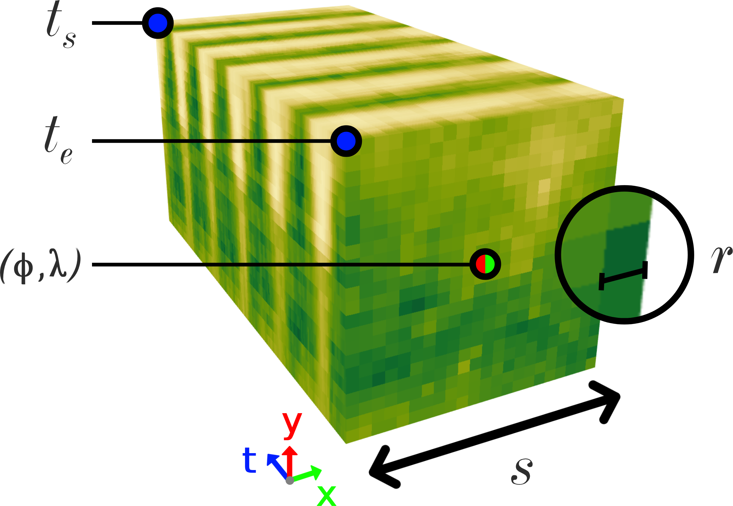
cubo characterises AI-focused ESDCs using the parameters described in Box 1 and illustrated in Fig. 1.
2.2 ESDC construction

cubo builds ESDCs through a series of steps using the above-mentioned parameters as user inputs (Fig. 2):
2.2.1 Bounding box calculation
cubo reprojects and into their respective Universal Transverse Mercator (UTM) zone coordinates, denoted as and . Additionally, cubo saves the Coordinate Reference System (CRS) as an attribute. These coordinates are then aligned to the nearest pair divisible by the spatial resolution , calculated as:
| (1) |
Here, represents either or , and is the adjusted coordinate. Next, the half-edge size in meters () is calculated as:
| (2) |
This rounding process ensures that the edge size is an even number. Finally, the bounding box coordinates are determined using:
| (3) |
Here, the tuples and denote the upper left and lower right coordinates of the bounding box, respectively.
2.2.2 ESDC creation
In its initial step, cubo accesses an STAC catalogue through an endpoint specified by the user, defaulting to the Planetary Computer STAC catalogue’s endpoint. Next, cubo feeds the bounding box parameters alongside and to pystac-client to retrieve all STAC items from a user-defined collection that intersect with these spatio-temporal constraints via a “search” operation. “kwargs” arguments are an option, enabling users to specify additional query parameters such as cloud cover percentage. Subsequently, these items are transferred to stackstac, combined with , the bounding box values, and the CRS. Additionally, the user can define the bands to retrieve. This process culminates in the generation of the ESDC as a “lazy” xarray object (Hoyer et al., 2017), chunked via dask (Rocklin, 2015), with the CRS specifically tailored to match the UTM zone associated with and .
| Attribute | Description |
|---|---|
| collection | Identifier of the collection within the STAC catalogue. |
| stac | Endpoint of the STAC catalogue used. |
| epsg | EPSG code of the ESDC’s CRS, corresponding to a specific UTM zone. |
| resolution | Spatial resolution, denoted by the value of . |
| edge_size | Edge size of the cube, given by the value of . |
| central_lat | Central latitude, indicated by . |
| central_lon | Central longitude, represented by . |
| central_y | UTM coordinate y, corresponding to . |
| central_x | UTM coordinate x, corresponding to . |
| time_coverage_start | Start timestamp of the ESDC, indicated by . |
| time_coverage_end | End timestamp of the ESDC, given by . |
2.2.3 Attributes writing
After the creation of the ESDC, cubo inscribes a set of global attributes on it, as outlined in Table 1. Additionally, cubo calculates the Euclidean distance between the coordinates of each pixel in the ESDC and the projected coordinate pair . This distance array is stored within the ESDC, adhering to the same spatial grids and dimensions, and can be accessed under the coordinate cubo:distance_from_center.
3 Showcase
We illustrate cubo’s efficacy through two distinct examples: 1) creating varied ESDCs with different parameters across multiple global locations, and 2) generating a standardised ESDC using different collections with identical parameters in the same location, all sourced from the Planetary Computer STAC catalogue.

In the first scenario, we harnessed various collections specialised for Earth system research (Fig. 3). The examples were generated across various locations globally, showcasing cubo’s versatility in handling data from any region. They also emphasise the importance of spatio-temporal context in a range of applications. For instance, the first three rows in Fig. 3 highlight potential uses in studying climate extremes and their effects on both the natural environment and human society. The first row features a Landsat-8 ESDC with a 30 m resolution, useful for detecting active fires and estimating burned areas. The second row shows a Sentinel-1 ESDC at 10 m resolution, ideal for flood detection and damage assessment. The third row introduces a MODIS-derived Gross Primary Production (GPP) dataset (17A2HGF), with a 500 m resolution, for analysing climate impacts on forest carbon sequestration. Lastly, the fourth row illustrates an annual ESDC from the ESA Climate Change Initiative (CCI) Land Cover (LC) product at 300 m resolution, beneficial as an additional input in various Earth system projects.

The ultimate goal of ESDCs is to integrate multiple datasets into a singular comprehensive analysis, enhancing our understanding and insights into the Earth system. In the second example, we focused on the same location as the third row of Fig. 3 (DE-Hai Eddy Covariance ICOS site at Hainich National Park, Germany) to create an extensive ESDC from various datasets, all retrieved with a 500 m spatial resolution and a 32-pixel edge size, covering data from 2022-08-01 to 2023-08-01. We gathered MODIS data on Surface Reflectance (SR), Land Surface Temperature (LST), GPP, Leaf Area Index (LAI), Fraction of Photosynthetically Active Radiation (FPAR), and Vegetation Indices (VIs). Fig. 4 displays these ESDCs, aligned with the same spatio-temporal grid. It’s noteworthy that datasets not matching the requested resolution (e.g. LST, VIs, and SR products) were automatically resampled by cubo, defaulting to the nearest neighbours method.
4 Conclusions
In this paper, we presented cubo, an open-source Python-based tool designed for the straightforward generation of ESDCs on demand. cubo simplifies the characterisation of AI-focused ESDCs, requiring minimal user input to create these ESDCs. cubo is versatile, and compatible with any COG collection within STAC. We anticipate cubo will be instrumental in various analytical processes requiring spatio-temporal context in Earth system research, with a particular emphasis on developing datasets for advanced AI tasks.
References
- Aybar et al. (2022) C. Aybar et al. Cloudsen12, a global dataset for semantic understanding of cloud and cloud shadow in sentinel-2. Scientific Data, 9(1), Dec. 2022. ISSN 2052-4463. doi: 10.1038/s41597-022-01878-2. URL http://dx.doi.org/10.1038/s41597-022-01878-2.
- Hoyer et al. (2017) S. Hoyer et al. xarray: N-d labeled arrays and datasets in python. Journal of Open Research Software, 5(1):10, Apr. 2017. ISSN 2049-9647. doi: 10.5334/jors.148. URL http://dx.doi.org/10.5334/jors.148.
- Mahecha et al. (2020) M. D. Mahecha et al. Earth system data cubes unravel global multivariate dynamics. Earth System Dynamics, 11(1):201–234, Feb. 2020. ISSN 2190-4987. doi: 10.5194/esd-11-201-2020. URL http://dx.doi.org/10.5194/esd-11-201-2020.
- Montero et al. (2023) D. Montero et al. Data cubes for earth system research: Challenges ahead. EarthArXiv, July 2023. doi: 10.31223/x58m2v. URL http://dx.doi.org/10.31223/X58M2V.
- Rocklin (2015) M. Rocklin. Dask: Parallel computation with blocked algorithms and task scheduling. In K. Huff and J. Bergstra, editors, Proceedings of the 14th Python in Science Conference, pages 130–136, 2015.
- Söchting et al. (2023) M. Söchting et al. Lexcube: Interactive visualization of large earth system data cubes. IEEE Computer Graphics and Applications, page 1–13, 2023. ISSN 1558-1756. doi: 10.1109/mcg.2023.3321989. URL http://dx.doi.org/10.1109/MCG.2023.3321989.
- Sumbul et al. (2019) G. Sumbul et al. Bigearthnet: A large-scale benchmark archive for remote sensing image understanding. In IGARSS 2019 - 2019 IEEE International Geoscience and Remote Sensing Symposium. IEEE, July 2019. doi: 10.1109/igarss.2019.8900532. URL http://dx.doi.org/10.1109/IGARSS.2019.8900532.