Scale-bridging within a complex model hierarchy for investigation of a metal-fueled circular energy economy by use of Bayesian model calibration with model error quantification

Abstract

Chemical reactor network (CRN) modeling is a promising approach for scale-bridging within a model hierarchy covering a huge range of scales from micro to macro in the scope of developing an innovative metal-fueled circular energy economy. This holds if valid information from CRNs, being models of reduced complexity, can be obtained on a much denser set of operating conditions than available from experiments and elaborated simulation methods like Computational Fluid Dynamics (CFD). An approach for CRN calibration including model error quantification from recent literature is used for developing a CRN model of a laboratory reactor for flash ironmaking, using data from the literature. By introducing a meta model of a CRN parameter, it has been possible to calibrate a simple CRN model on an extended set of operating conditions with satisfactory results. This way, the employed coupled calibration and uncertainty quantification framework seems promising for the task of scale-bridging in the model hierarchy under investigation. Challenges for the further extension of the present work into that direction are discussed.

Keywords Chemical reactor networks  $\cdot$ Scale-bridging  $\cdot$ Uncertainty quantification  $\cdot$ chemical energy carriers  $\cdot$ Model hierarchy  $\cdot$ Complexity-reduction

Abbreviations

ABC	Approximate Bayesian Computation
a.u.	arbitrary units
CFD	Computational Fluid Dynamics
CRN	Chemical Reactor Network
OP	Operation Point
PDF	Probability Density Function
PFR	Plug Flow Reactor
PSR	Perfectly Stirred Reactor

Notation

$\bm{\alpha}$	Parameter vector for parametrization of model error
$\bm{\tilde{\alpha}}$	$\bm{\tilde{\alpha}}$ = ($\bm{\lambda}$,$\bm{\alpha}$)
$B$	Image space of $g$ and $f$, $B\subset\mathbb{R}$, $B=g(S)=f(S\times\mathbb{R}^{d})$
$D$	Data set used for calibration, generated from $g$
$d$	Dimension of model parameter vector $\lambda$
$\delta$	(Unknown) discrepancy between $g$ and $f$
$\epsilon$	Data error occuring in the evaluation of $g$
$f$	Low-fidelity parametrized model to be calibrated
$g$	High-fidelity model $g$ used for calibration of $f$
$\eta$	Tolerance parameter in the ABC likelihood construction
$\bm{\lambda}$	Vector of parameters to be calibrated in the model $f$
$\bm{\Lambda}$	Random vector representing the model parameters augmented with model error
	($\bm{\Lambda}(\bm{\alpha},\bm{\xi})=\bm{\lambda}+\bm{\delta}(\bm{\alpha},\bm{\xi})$)
$\mu$	Mean of a random quantity
$N$	Dimensionality of design space
$\pi_{Q}(\cdot)$	Probability density function with respect to a random quantity Q
$S$	Design space, $D\subsetneq S\times B\subset\mathbb{R}^{N}\times B$
$\sigma$	Standard deviation of a random quantity
$\mathbf{x}$	Vector of observables/oeprating conditions ($\mathbf{x}\in S$)
$\bm{\xi}$	Vector of independent identically distributed random variables
$y$	Model output observable ($y\in B)$

Nomenclature

Name	Meaning throughout this work	Example
Operating condition	A set of parameters that can be	Gas and solid mass flows provided to a reactor
	adjusted in experiments
	and is not dependent on a model.
	Serves as input to models.
Operation point	A specific, labeled set of operation	see Table 3
	conditions used within
	the study, mostly accompanied
	with a measurement result
Model parameter	Parameters specific to a certain model.	CRN: reactor temperatures, volumes,….
	The calibration procedures presented
	in this work are for calibration
	of (a subset of) model parameters
Reactor	Is used ambiguously as term	(1) Laboratory reactor for flash ironmaking
	for a full chemical reactor (1)
	or the modeling blocks	(2) PFR and PSR models (see Section 2.1)
	within a CRN model (2)
Design space	Subset of the space of operating	Figure 3
	conditions for which a valid (CRN)
	model shall be calibrated.

1 Introduction

Metal fuels and especially iron are recently gaining attention as carbon-neutral chemical energy carriers for storing and transporting renewable electricity [1, 2, 3] due to advantageous properties of the considered metals, such as abundance and volumetric energy density. In a circular process, energy from renewable energy sources is stored in form of iron through reduction of iron oxides using green hydrogen as reducing agent. The iron particles can then be transported to locations with high energy demand, where energy is released in form of heat through combustion with oxygen, producing iron oxide particles that can be returned to the reduction site to close the cycle.

Until ready for deployment, the investigation of such a novel concept relies on various different scales ranging from fundamental research on the micro- and nanoscale [4, 5, 6, 7], via mesoscale laboratory and pilot systems [8, 9, 10, 11], up to global scale investigations such as techno-economic and lifecycle assessments [12, 13] or political and economical considerations [14, 15, 16]. Information transfer within this model hierarchy on a huge range of scales is crucial for proper model analyses and for making the technology ready for application in a time-frame limited by the urgence of the energy transition. Mesoscale applications are of particular importance for scale-bridging. On the mesoscale, chemical reactors from laboratory to pilot industrial scales are investigated experimentally and with modeling approaches and simulations.

In the context of reactor modeling, Computational Fluid Dynamics (CFD) simulations are typically used for detailed reactor simulations that reveal deep understanding of the physical phenomena in the reactor like global and local fluid dynamics, turbulence-reaction interactions and flame structures. However, performing CFD simulations is computationally costly. Experiments are costly, too, and usually take a long time to be accomplished when prior construction work is accounted for. Experiments and CFD simulations yield crucial information and understandings of the overall reactor behavior. To a certain extent, these methods also yield information on the chemical conversion of species, the latter however being restricted to certain species, depending on the case, and on the available measurement techniques or computational resources.

Scale- and complexity-reduced models try to find a trade-off between the (computational) cost and the considered level of detail and hence represent a bridge between detailed expensive simulation models and the need for readily accessible information on the global scale. Chemical Reactor Networks (CRNs) [17] are an instance for scale-reduced models that are based on CFD or experimental results, or both. CRNs are graph-like structures composed of modeling blocks, which employ strongly simplified flow models, while enabling the incorporation of reaction mechanisms that are partially even more complex than those tractable in CFD simulations [17, 11]. The computational effort of solving CRNs depends on the applied reaction mechanism and the number of reactor compartments, their structure within the network as well as the underlying reactor description. Nevertheless, using CRNs leads to a great reduction of computation time and resources in comparison to CFD models. CRN solutions can be computed on personal computers in less than seconds to a few hours, while CFD computations usually take days to weeks on high performance clusters [17].

However, the construction of CRNs is usually based on CFD or experimental results. In order for them to be used as a scale-bridging tool in large-scale mathematical and thermodynamic models, data is needed on a set of operating conditions that is much larger than the available data set from CFD or experiments, which implies that CRNs need to be validly constructed and solved for those conditions where no CFD or experimental data exists. A promising approach to analyse and exploit the predictive capacity of CRNs has recently been introduced by Savarese et al. [18], who exemplified the calibration of a CRN model to a set of CFD data points within a Bayesian model-to-model-calibration framework, including model error quantification as proposed in [19, 20], for an ammonia-fueled micro-turbine.

The objective of the present work is to transfer this approach to the present setting of scale-bridging within a metal-fueled energy circular economy and to preliminarily assess the usability of the calibration framework within this scope. This comes along with the challenge of using experimental data from the literature for which operation conditions corresponding to the data being spread irregularly and unevenly in the design space.

While it seems promising for the iron combustion to take place in retrofitted coal-fired power plants [3], the emission-less reduction of iron oxides requires new technology, whose development however goes in line with various approaches for the development of "green" steel production.

Flash ironmaking [21] is a novel technology that has several advantages over conventional iron production concepts like blast furnace processes [21], and is also a promising candidate when considering iron as energy carrier within a circular economy [12]. In an extensive study, Sohn and co-workers have studied this process with applications on various scales, from kinetic development in laminar flow reactors, via laboratory and pilot experimental applications, to CFD simulations from the laboratory to industrial scale [22, 23, 24, 25, 26, 27, 28, 29, 21]. This case has been chosen for testing the calibration approach due to data being available for different scales and the complexity being lower than in many test cases on the combustion site of the energy cycle. Within the scope of the present work, a CRN model is developed and calibrated for modeling the laboratory reactor by Sohn, using the experimental data summarized in [21] for CRN construction, calibration and validation. This shall be extended to the other scales in future work.

The paper is structured as follows. Section 2 summarizes the theoretic concept of chemical reactor network modeling, and model-to-model calibration with embedded model error in the framework of Bayesian inference, based on the work by Sargsyan et al. [19, 20]. Section 3 describes the developed workflow used to employ the theoretical concepts to the use case, which is similar to the workflow introduced by Savarese et al. [18]. Further details on the testcase of CRN calibration for iron oxide reduction will be provided in Section 4. The CRN construction and obtained calibration results will be presented and discussed in Section 5 and the results will be related to the objectives and the scope of this work in Section 6. Lastly, Section 7 concludes this work with final remarks and an outlook on future work.

2 Theoretical Background

The aim of the present work is to calibrate a Chemical Reactor Network (CRN) model on a given set of operating conditions, the design space. In order to assess the validity of the obtained calibrated model, it is crucial to be able to quantify uncertainties of the model output and, where possible, investigate and mitigate their origin. Because of this, we employ the embedded model error approach suggested by Sargsyan et al.[19], which has already been exemplified for CRNs by Savarese et al.[18].

In the following sections, we will introduce the key ideas of that approach relevant to understanding our application and also the calibration procedure, mostly following the work of Sargsyan et al. [19, 20]. Before that, we will shortly introduce the concept of chemical reactor networks.

2.1 Chemical Reactor Network Modeling

Chemical reactor networks (CRNs) are graph-like mathematical models of a chemical reactor, built of modeling units representing spatial regions of the reactor, which are interconnected by streams holding the information about the mass flows between the compartments. The unit boundaries are determined by the physical properties within the reactor like temperature distribution and flow structure, leading to the definition of functional compartments [17].

Figure 1: Generic chemical reactor network including ideal reactors, mixing and splitting units. Adapted from [17].

The main units of a CRN are ideal steady-state reactor models that combine a simplified flow assumption with a detailed description of chemical reactions. A generic reactor network is depicted in 1. Regions of strong mixing are approximated by a 0D model, which assumes infinitely fast and perfect mixing of the species with mass fraction $Y_{i}$, the perfectly stirred reactor (R1). The chemical system is defined by the density $\rho$ of the mixture, the molecular weight $\mathrm{MW_{i}}$, the formation rate $\dot{\omega}_{i}$ of the reactants and the residence time $\tau$ of the reactor [17]:

$$\frac{dY_{i}}{dt}=\frac{Y_{i}^{in}-Y_{i}}{\tau}+\frac{\mathrm{MW}_{i}\dot{\omega}_{i}}{\rho}.$$ (1)

The 1D plug flow reactor model (R2) considers straight flow patterns, assumes perfect radial mixing and neglects mixing in the axial direction. Thus, the species conservation equations along the reactor coordinate $z$ are formulated as follows [17]:

$$\frac{dY_{i}}{dz}=\frac{\mathrm{MW}_{i}\dot{\omega}_{i}}{\rho v}$$ (2)

with the fluid velocity $v$. Together with mixing (M1) and splitting units (S1) to model the distribution of the flow between the different reactors, the CRN structure is fully determined. The solution of a CRN model is a vector of mass fractions for the given species and every stream and reactor of the CRN. Here, however, usually the outlet stream of the complete reactor, i.e. the stream leaving the network, is of interest.

The modeling parameters of a CRN are the overall structure and number of modeling blocks and several parameters within each modeling block, like the temperature, volumes or residence times. The modeling blocks are assumed to be isothermal throughout this work, which is often the case for CRNs. The enthalpy equations having the most influence on temperature are usually solved within the CFD computation and the resulting temperature fields are then used for the CRN construction. A subset of the CRN model parameters will be calibrated within this work, using the calibration framework introduced in the next sections.

2.2 Model-to-Model-calibration with embedded model error

Consider a set $S\subset\mathbb{R}^{N},\ N\in\mathbb{N}$ of physical observables, which we will refer to as the design space. In our case, these observables are operating conditions like mass flows or pressure, on which the CRN depends. The design space defines the bounds within which a valid model is to be calibrated.

Consider a model $g\colon S\rightarrow B\subset\mathbb{R},\ \mathbf{x}\longrightarrow y$, mapping the design space to some observable $y$, which is throughout this work assumed to be scalar.

This model is referred to as high-fidelity, or even truth model [19], which essentially means that $g$ is assumed to have negligible model error, compared to another model $f$ that shall be calibrated on $S$. On the other hand, $g$ is in general expensive to be evaluated such that only a finite set of data generated from $g$ is available, which is denoted by $D=\{\left(\mathbf{x}^{(i)},y^{(i)}\right)\}_{i=1}^{L}$, where $L$ is the number of evaluations of $g$ and $\mathbf{x}^{(i)}\in S$ is the $i$-th operation condition for which $g$ is evaluated. In general, there can be a data error while evaluating $g$, leading to

$$y^{(i)}=g(\mathbf{x}^{(i)})+\epsilon^{(i)},$$ (3)

where $\epsilon^{(i)}$ is the data error associated to the evaluation of $y^{(i)}$. In the context of Chemical Reactor Networks, the data set $D$ is usually obtained from experiments or Computational Fluid Dynamics (CFD) simulations.

The model to be calibrated is a parametrized model $f\colon S\times\mathbb{R}^{d}\rightarrow B\subset\mathbb{R},\ (\mathbf{x},\bm{\lambda})\longrightarrow y$, where $\bm{\lambda}=(\lambda_{1},...,\lambda_{d})$ is the vector of parameters being specific to the model $f$. In the CRN context this can for instance be reactor temperatures or volumes. The vector $\bm{\lambda}$ provides the degrees of freedom for the calibration of $f$ to the data set $D$. The model $f$ is referred to as low-fidelity model as it has a non-negligible model error, as will be introduced next. Note that $f$ is assumed to be surjective and, more strictly, it is assumed that for every $y\in B$ and every $\mathbf{x}\in S$ there is a $\bm{\lambda}\in\mathbb{R}^{d}$ such that $f(\mathbf{x},\bm{\lambda})=y$.
In addition to the measurement noise represented by $\epsilon^{(i)}$, there is a model discrepancy between the high-fidelity model $g(\mathbf{x})$ and the lower fidelity model $f(\mathbf{x},\bm{\lambda})$, defined as $\delta(\mathbf{x})=g(\mathbf{x})-f(\mathbf{x},\bm{\lambda})$. This results in the following expression for the relation of the lower fidelity model $f$ to the measurements $(\mathbf{x}^{(i)},y^{(i)})$:

$$y^{(i)}=f(\mathbf{x}^{(i)},\bm{\lambda})+\delta(\mathbf{x}^{(i)})+\epsilon^{(i)}.$$ (4)

One way of dealing with this explicit formulation of the model error $\delta(\mathbf{x})$ as presented in [20] is to embed the model error within the model $f$. For this purpose, an additive term $\bm{\delta}$ is added to the model parameters $\bm{\lambda}$ in order to account for the model discrepancy, resulting in the term $f(\mathbf{x},\bm{\lambda}+\bm{\delta})$. As we will shortly see, the additive term $\bm{\delta}$ will be represented by a polynomial chaos expansion parameterized by parameters $\bm{\alpha}$ and expressed in terms of a random vector $\bm{\xi}$, such that the model can be rewritten as

$$y^{(i)}\approx f(\mathbf{x}^{(i)},\bm{\lambda}+\bm{\delta}(\bm{\alpha},\bm{\xi}))+\epsilon^{(i)}\ \text{for}\ i=1,\dots,L.$$ (5)

In the following, the parameters $\bm{\lambda}$ and $\bm{\alpha}$ are combined into $\bm{\tilde{\alpha}}=(\bm{\lambda},\bm{\alpha})$ and the random quantity representing the parameters $\bm{\lambda}$ and the additive uncertain model error $\bm{\delta}(\bm{\alpha},\bm{\xi})$ is denoted by $\bm{\Lambda}(\bm{\tilde{\alpha}})=\bm{\lambda}+\bm{\delta}(\bm{\alpha},\bm{\xi})$, resulting in

$$y^{(i)}\approx f(\mathbf{x}^{(i)},\bm{\Lambda}(\bm{\tilde{\alpha}}))+\epsilon^{(i)}\ \text{for}\ i=1,\dots,L.$$ (6)

It is important to note that the original calibration for $\bm{\lambda}$ has been turned into a parameter estimation problem for $\bm{\tilde{\alpha}}$ by explicitly embedding the model error. The result of the calibration is a PDF associated to a random quantity $\bm{\Lambda}$, which in turn yields a random prediction $f(\mathbf{x},\bm{\Lambda})$, the latter being characterized by a PDF, too. The random prediction $f(\mathbf{x},\bm{\Lambda})$ and its associated PDF can in the end be interpreted as an approximation of the probability distribution of the "true" prediction $g(\mathbf{x})$.

2.3 Bayesian Inference for Model Calibration

Bayesian and frequentist statistics represent two distinct approaches used for statistical inference, that differ in the way of interpreting probability and using observed data, leading to different inference concepts. While the frequentist approach views probabilities as the long-term relative frequency of occurrence of a certain event, in the Bayesian approach probabilities represent beliefs that are updated based on observations.
Bayesian inference incorporates prior knowledge on parameters $\bm{\tilde{\alpha}}$, i.e. it views $\bm{\tilde{\alpha}}$ as random vector that is distributed according to some probability distribution $\mathcal{P}(\bm{\tilde{\alpha}})$, and computes a posterior distribution $\mathcal{P}(\bm{\tilde{\alpha}}|D)$ of the parameters, given some observations $D$, using Bayes’ Theorem

$$\mathcal{P}(\bm{\tilde{\alpha}}|D)=\frac{\mathcal{P}(D|\bm{\tilde{\alpha}})\cdot\mathcal{P}(\bm{\tilde{\alpha}})}{\mathcal{P}(D)}.$$ (7)

Here, $\mathcal{P}(D|\bm{\tilde{\alpha}})$ is the likelihood function that represents the probability of the observations given specific parameter values $\bm{\tilde{\alpha}}$, whereas $\mathcal{P}(D)$, sometimes referred to as evidence, is the probability of the observations. Note that $\mathcal{P}(D)$ is independent of the realization of $\bm{\tilde{\alpha}}$ and hence can be seen as a normalizing factor.
In the presented setting of model-to-model calibration, the goal is to determine parameters $\bm{\tilde{\alpha}}$ that best describe the observed data $D$. Thus, computing the posterior distribution $\mathcal{P}(\bm{\tilde{\alpha}}|D)$ provides the desired knowledge about $\bm{\tilde{\alpha}}$ in terms of the probability that, given the observations $D$, the model is parameterized by $\bm{\tilde{\alpha}}$. Hence the model-to-model calibration problem can be solved by performing Bayesian inference for the parameters $\bm{\tilde{\alpha}}$.
In the following, the general calibration procedure will be presented, including how the different components (e.g. prior, likelihood) are constructed in order to perform Bayesian inference for obtaining the posterior distribution.

2.4 Calibration Procedure

In Table 1, an overview on the calibration procedure is given. The order of some of the steps is interchangeable, however, for the purpose of orientation, the order has been chosen as presented here. In the present section, the theoretical background of the calibration steps will be explained in the order given in the table.

Table 1: Overview of the calibration procedure employed

1.	Parametrization of model error to obtain the parameter set $\bm{\tilde{\alpha}}$
2.	Definition of priors
3.	Choose likelihood type (here: ABC)
	3.1. ABC: Choose parameter $\eta$
4.	Sampling of $\bm{\tilde{\alpha}}$ with the Markov Chain Monte Carlo (MCMC) method
5.	For each $\bm{\tilde{\alpha}}$: Calculation of likelihood.
	5.1. Model error embedding: create PCE representation of $f(\mathbf{x},\bm{\Lambda}(\bm{\tilde{\alpha}}))$
	5.2. ABC: Calculate mean and variance of $f(\mathbf{x},\bm{\Lambda}(\bm{\tilde{\alpha}}))$ (straight-forward with PCE representation created in 5.1.)
	5.3. ABC: Calculate $L_{ABC}(\bm{\tilde{\alpha}})$ with Equation (22)
6.	Obtain posterior value for $\bm{\tilde{\alpha}}$, $\mathcal{P}(\bm{\tilde{\alpha}}|D)\propto\mathcal{P}(D|\bm{\tilde{\alpha}})\mathcal{P}(\bm{\tilde{\alpha}})=L_{ABC}(\bm{\tilde{\alpha}})\mathcal{P}(\bm{\tilde{\alpha}})$
7.	Continue sampling of $\bm{\tilde{\alpha}}$ according to posterior value obtained.
	7.1. Back to 5., until maximum MCMC step number is reached.

2.4.1 Polynomial chaos expansions of the parameters augmented with model error

Within the Bayesian inference approach applied in this work, Polynomial Chaos Expansions have an important role for both, model error embedding, and enhancing the numerical tractability.

Polynomial Chaos expansions are feasible representations of random quantities such as the model parameters augmented by model error, i.e. $\bm{\Lambda}(\bm{\tilde{\alpha}})$. Consider a polynomial basis $\{\psi^{(i)}(\xi)|\ i\in\mathbb{N}_{0}\}$ with $\deg(\psi^{(i)})=i$. Assume that $\xi$ is a random variable supported on $[-1,1]$ and that the polynomial basis is orthogonal with respect to the PDF of $\xi$ given by $\pi(\xi)$, that is

$$\langle\psi^{(i)},\psi^{(j)}\rangle:=\int_{[-1,1]}\psi^{(i)}(\xi)\psi^{(j)}(\xi)\pi(\xi)d\xi=\delta_{ij}\langle\psi^{(i)},\psi^{(i)}\rangle,$$ (8)

where $\delta_{ij}$ is the Kronecker delta.

Furthermore, consider a maximum polynomial order $p\in\mathbb{N}$, a set of multi-indices

$$K=\{\mathbf{k}=(k_{1},...,k_{d})\in\mathbb{N}^{d}\ |\ |\mathbf{k}|=\sum_{j=1}^{d}k_{j}\leq p\}$$ (9)

and a set of coefficients $\{a_{\mathbf{k}}|\mathbf{k}\in K\}$. Let $\bm{\xi}=(\xi_{1},\dots,\xi_{d})$ be a vector of i.i.d. variables. Then a general finite-variance random quantity $\zeta$ can be represented as [19, 30, 31]:

$$\zeta=\sum_{\ell\in\mathbb{N}}a_{\mathbf{k}_{\ell}}\Psi_{\mathbf{k}_{\ell}}(\bm{\xi}),$$ (10)

where $\Psi_{\mathbf{k}}(\bm{\xi})=\Pi_{j=1}^{d}\psi^{(k_{j})}(\xi_{j})$. In numerical practice, a truncation up to an order $p$ is used to approximate $\zeta$ [30, 31, 32] according to

$$\zeta\approx\sum_{\ell=1}^{P}a_{\mathbf{k}_{\ell}}\Psi_{\mathbf{k}_{\ell}}(\bm{\xi}),$$ (11)

involving $P=\frac{(p+d)!}{p!d!}=|K|$ terms. Note that each $\Psi_{\mathbf{k}}(\bm{\xi})$ is a product of the basis polynomials, where the maximum sum of all polynomial orders of the $d$ polynomials is $p$ and $\zeta$ is the sum of all possible $\Psi_{\mathbf{k}}(\bm{\xi})$ fulfilling this constraint, each weighted with a coefficient $a_{\mathbf{k}_{\ell}}$.

This way, the $j$-th augmented model parameters $\Lambda_{j}(\bm{\tilde{\alpha}},\bm{\xi})$ can be represented via Polynomial Chaos Expansion [20] as

$$\Lambda_{j}(\bm{\tilde{\alpha}},\bm{\xi})=\lambda_{j}+\delta_{j}(\bm{\alpha},\bm{\xi})\approx\lambda_{j}+\sum_{\ell=1}^{P}\alpha_{\mathbf{k}_{\ell,j}}\Psi_{\mathbf{k}_{\ell}}(\bm{\xi})=\tilde{\alpha}_{0,j}+\sum_{\ell=1}^{P}\tilde{\alpha}_{\mathbf{k}_{\ell,j}}\Psi_{\mathbf{k}_{\ell}}(\bm{\xi}).$$ (12)

In Section 2.4.5, the PCE approach will be further employed for creating surrogate models of $f(\mathbf{x},\bm{\Lambda}(\bm{\tilde{\alpha}}))$, and in Section 2.5, a deterministic approach with similar structure will be employed for creating surrogate models of $f(\mathbf{x},\bm{\lambda})$, since surrogate models usually have a higher numerical tractability than the model itself.

2.4.2 Definition of priors

In order to calculate the posterior distribution $\mathcal{P}(\bm{\tilde{\alpha}}|D)$, the prior $\mathcal{P}(\bm{\tilde{\alpha}})$ needs to be defined. The prior contains the knowledge on the probability distribution of $\bm{\tilde{\alpha}}$ before the calibration. Throughout the present work, bounded uniform priors will be employed, i.e.

$$\mathcal{P}(\tilde{\alpha}_{i})=\begin{cases}\textrm{const},&a_{i}<\tilde{\alpha}_{i}<b_{i},\\ 0,&\textrm{else},\end{cases}$$ (13)

where $\tilde{\alpha}_{i}$ is the $i$-th component of $\bm{\tilde{\alpha}}$. The respective bounds $a_{i}$ and $b_{i}$ are determined by consideration of the physical knowledge on the parameters. This way, no additional prior knowledge is incorporated into the calibration, which is desired in the present work.

2.4.3 Calculation of likelihood

The calculation of a proper likelihood $L_{D}(\bm{\tilde{\alpha}})=\mathcal{P}(D|\bm{\tilde{\alpha}})$ is a central step in the inference procedure. Given a parametrization $\bm{\tilde{\alpha}}$ of the random parameter set $\bm{\Lambda}(\bm{\tilde{\alpha}})$, it yields the probability that the data set $D$ will be obtained when the model $f$ is evaluated at the operation conditions given in $\mathbf{x}$.

However, the latter statement can be interpreted in different ways, depending on how exactly the likelihood is calculated. This will be illustrated in the following.

Sargsyan and coworkers provide a detailed overview of the different ways the likelihood can be modeled, including the features and shortcomings of the different approaches [19, 20]. This given, only a few central aspects will be summarized, especially focusing on the proper interpretation of the results that are obtained when choosing a likelihood type.

The first important point is the following distinction: Either it is required that there exists a realisation of the parameter vector $\bm{\Lambda}(\bm{\tilde{\alpha}})$ such that $f(\mathbf{x},\bm{\Lambda}(\bm{\tilde{\alpha}}))=g(\mathbf{x})$ for every $\mathbf{x}\in S$. Otherwise, it is sufficient that for each $\mathbf{x}\in S$, there is a realisation of $\bm{\Lambda}(\bm{\tilde{\alpha}})$ such that $f(\mathbf{x},\bm{\Lambda}(\bm{\tilde{\alpha}}))=g(\mathbf{x})$, but here the value of $\bm{\Lambda}(\bm{\tilde{\alpha}})$ can be different for every $\mathbf{x}$. This distinction is incorporated into the likelihood evaluation by either requiring that there is a realisation $\bm{\Lambda}(\bm{\tilde{\alpha}})$ with nonzero probability density such that $f(\mathbf{x}^{(i)},\bm{\Lambda}(\bm{\tilde{\alpha}}))=y^{(i)}$ for every $\left(\mathbf{x}^{(i)},y^{(i)}\right)\in D$ for $\bm{\tilde{\alpha}}$ to have nonzero likelihood, or only requiring that for every $\left(\mathbf{x}^{(i)},y^{(i)}\right)\in D$, there is a realisation $\bm{\Lambda}(\bm{\tilde{\alpha}})$ with nonzero probability density such that $f(\mathbf{x}^{(i)},\bm{\Lambda}(\bm{\tilde{\alpha}}))=y^{(i)}$, if $\bm{\tilde{\alpha}}$ is to be assigned nonzero likelihood.

In the first case, the $L$-dimensional PDF $\pi_{\mathbf{f}(\bm{\tilde{\alpha}},\bm{\xi})}(\mathbf{\cdot})$ with $\mathbf{f}(\bm{\tilde{\alpha}},\bm{\xi})\coloneqq\left(f(\mathbf{x}^{(1)},\bm{\tilde{\alpha}},\bm{\xi})+\epsilon^{(1)},...,f(\mathbf{x}^{(L)},\bm{\tilde{\alpha}},\bm{\xi})+\epsilon^{(L)}\right)$ has to be computed and evaluated at $\mathbf{y}\coloneqq\left(y^{(1)},...,y^{(L)}\right)$, with $(\mathbf{x}^{(i)},y^{(i)})\in D$. This is referred to as the full likelihood by Sargsyan et al. [19, 20] and, if no data error is considered ($\epsilon^{(i)}=0\ \textrm{for}\ i=1,...,L$), it is in general zero for any $\bm{\tilde{\alpha}}$, except the trivial case in which there exists a parameter vector $\bm{\Lambda}(\bm{\tilde{\alpha}})$ such that $f(\cdot,\bm{\Lambda}(\bm{\tilde{\alpha}}))=g(\cdot)$. If a data error is considered, it becomes finite, but the $L$-dimensional PDF remains computationally intractable in many cases [19, 20].

In the second case, the likelihood is calculated as the product of the marginal PDFs for each $\left(\mathbf{x}^{(i)},y^{(i)}\right)\in D$, that is [19, 20]

$$L_{D}(\bm{\tilde{\alpha}})=\Pi_{i=1}^{L}\pi_{\left(f(\mathbf{x}^{(i)},\bm{\tilde{\alpha}},\bm{\xi})+\epsilon^{(i)}\right)}(y^{(i)}).$$ (14)

From a stochastic point of view, if a "full" likelihood is employed, the components of $\mathbf{f}$ are treated as dependent variables, whereas if the "marginal" likelihood is employed, they are considered independent.

The marginal likelihood is in general nonzero for many samples of $\bm{\tilde{\alpha}}$ and much more tractable from the computational point of view, as $L$ one-dimensional PDFs have to be calculated instead of one $L$-dimensional PDF. Still, even the marginal likelihood (14) can be too demanding in terms of computational resources, which is why several moment-based approximations are suggested by Sargsyan et al. [19, 20], one of them being introduced below and employed for the computations that have been conducted for the present work.

Before this, a short comment shall be made on the interpretation of results when a "full" or "marginal" likelihood type is used. Especially, if no data error is considered, the marginal likelihood is more than just an approximation of the full likelihood. In the end, it (approximately) yields what the model error approach aims for: A PDF over a random parameter vector $\bm{\Lambda}$, parametrized by a vector $\bm{\tilde{\alpha}}$, whose value for a certain realisation $\bm{\Lambda}^{*}$ can for each single $\mathbf{x}^{*}\in S$ be interpreted as the probability that $\bm{\Lambda}^{*}$ is the "true" $\bm{\Lambda}$, i.e. the one for which it holds $f(\mathbf{x}^{*},\bm{\Lambda}^{*})=g(\mathbf{x}^{*})$. As for any $\mathbf{x}\in S$, the "true" realisation can however not be known, especially if $\mathbf{x}\notin D\cap S$, the PDF $\pi_{f(\mathbf{x},\bm{\tilde{\alpha}},\bm{\xi})}(\mathbf{\cdot})$ describes the probability on the "true" value searched for.

The term approximately here comes from the fact that there is no infinite data set $D$ used for the calibration, no infinite set of samples on $\bm{\tilde{\alpha}}$ whose likelihood can be calculated, and that only PDFs are sampled that fit the way the parametrization of the embedded model error has been done, e.g. limited-order PCEs as introduced in Section 2.4.1. Especially if no data error is considered, it is not an approximation of the full likelihood, which usually equals zero. Even, for the full likelihood, the model error concept is not useful, as the model error is zero while the likelihood is not and vice versa.

As mentioned above, Sargsyan and coworkers recommend the use of moment-based likelihoods, which are computationally more tractable than sampling of the full or marginal PDFs [19, 20]. One of them, Approximate Bayesian Computation (ABC) is employed in this work and presented in the following.

Approximate Bayesian Computation (ABC)

(lala)

In Approximate Bayesian Computation (ABC), the likelihood is approximated by a direct measure for comparing the statistics, usually the mean $\mu$ and standard deviation $\sigma$, of the model response to the actual data set $D$.

This means, for each $\left(\mathbf{x}^{(i)},y^{(i)}\right)\in D$, i = 1,…, L, it is required that

$$\mu^{i}_{f}(\bm{\tilde{\alpha}})\approx y^{(i)},$$ (15)

$$\sigma^{i}_{f}(\bm{\tilde{\alpha}})\approx|y^{(i)}-\mu^{i}_{f}(\bm{\tilde{\alpha}})|.$$ (16)

Here,

$$\mu^{i}_{f}(\bm{\tilde{\alpha}})=\int_{[-1,1]^{d}}f\left(\mathbf{x}^{(i)},\bm{\tilde{\alpha}},\bm{\xi}\right)\pi(\bm{\xi})d\bm{\xi},$$ (17)

$$\sigma^{i}_{f}(\bm{\tilde{\alpha}})=\left[\int_{[-1,1]^{d}}\left(f\left(\mathbf{x}^{(i)},\bm{\tilde{\alpha}},\bm{\xi}\right)-\mu^{i}_{f}(\bm{\tilde{\alpha}})\right)^{2}\pi(\bm{\xi})d\bm{\xi}\right]^{\frac{1}{2}}.$$ (18)

To this end, a distance function $\bm{\rho}$ can then be defined as

$$\bm{\rho}(\bm{\tilde{\alpha}})=\left(|y^{(1)}-\mu^{1}_{f}(\bm{\tilde{\alpha}})|,||y^{(1)}-\mu^{1}_{f}(\bm{\tilde{\alpha}})|-\sigma_{f}^{1}(\bm{\tilde{\alpha}})|,...,|y^{(L)}-\mu^{L}_{f}(\bm{\tilde{\alpha}})|,||y^{(L)}-\mu_{f}^{L}(\bm{\tilde{\alpha}})|-\sigma_{f}^{L}(\bm{\tilde{\alpha}})|\right),$$ (19)

which is weighted by a kernel function. Often, a Gaussian type kernel is used [19]:

$$K(\bm{\rho}):=\frac{1}{\sqrt{2\pi}}\exp\left(-\frac{||\bm{\rho}||_{2}^{2}}{2}\right).$$ (20)

The likelihood then is defined as [19]

$$L(\bm{\rho})=\frac{1}{\eta}K\left(\frac{\bm{\rho}}{\eta}\right),$$ (21)

where $\eta$ is a tolerance parameter that determines how strict the moments have to match.

In total, this yields the following ABC-likelihood:

$$L_{ABC}(\bm{\tilde{\alpha}})=\frac{1}{\eta\sqrt{2\pi}}\scalebox{1.2}{$\prod_{i=1}^{L}$}\exp\left(\frac{(y^{(i)}-\mu_{i}(\bm{\tilde{\alpha}}))^{2}+(|y^{(i)}-\mu_{f}^{i}(\bm{\tilde{\alpha}})|-\sigma_{f}^{i}(\bm{\tilde{\alpha}}))^{2}}{2\eta^{2}}\right).$$ (22)

2.4.4 Markov Chain Monte Carlo

Markov Chain Monte Carlo (MCMC) methods are widely used for sampling from probability distributions, for which straight forward sampling methods are difficult. Especially in the context of Bayesian inference, MCMC is used to sample from the desired posterior distribution $\mathcal{P}(\bm{\tilde{\alpha}}|D)$.
MCMC combines Monte Carlo sampling with the construction of a Markov chain such that the stationary distribution of the Markov chain is the distribution from which the samples are desired.
The general MCMC procedure is summarized in the Metropolis-Hastings algorithm [33, 34]. It relies on choosing new states based on some proposal distribution and accepting or rejecting the proposed states based on an acceptance ratio.
Within this acceptance ratio, the desired distribution has to be evaluated at the current state and at the proposed state. However, due to the ratio construction it suffices to evaluate a distribution proportional to the desired distribution, since the proportionality factor cancels in the ratio. Thus, for sampling the posterior distribution in the setting of Bayesian inference, it suffices to evaluate the product of likelihood and prior as $\mathcal{P}(\bm{\tilde{\alpha}}|D)\propto\mathcal{P}(D|\bm{\tilde{\alpha})}\mathcal{P}(\bm{\tilde{\alpha}}).$
Extensions of the initial Metropolis-Hastings algorithm aim at improving the convergence behaviour of the algorithm. This is for example done by adaptively updating the proposal distribution, which results in an adaptive MCMC algorithm, rather than keeping it fixed throughout the entire process ([35], [36]).

2.4.5 Predictive Moment Estimation

The ABC likelihood construction requires only the computation of the predictive means $\mu_{f}^{i}(\bm{\tilde{\alpha}})$ and standard deviations $\sigma_{f}^{i}(\bm{\tilde{\alpha}})$, whereas the full PDF is not necessary. Using PCEs of the model outputs $f(\mathbf{x}^{(i)},\bm{\Lambda}(\bm{\tilde{\alpha}},\bm{\xi}))$, this information can be easily obtained as follows [19, 20]: A PCE is constructed for each input $\mathbf{x}^{(i)}$ according to

$$f(\mathbf{x}^{(i)},\bm{\Lambda}(\bm{\tilde{\alpha}},\bm{\xi}))\approx\sum_{\ell=1}^{P}f_{\ell}(\mathbf{x}^{(i)},\bm{\tilde{\alpha}})\Psi_{\ell}(\bm{\xi}),$$ (23)

where the coefficients $f_{\ell}(\mathbf{x}^{(i)},\bm{\tilde{\alpha}})$ are computed via integration by quadrature as

$$f_{\ell}(\mathbf{x}^{(i)},\bm{\tilde{\alpha}}) =\frac{1}{\|\Psi_{\ell}\|^{2}}\int_{\bm{\xi}}f(\mathbf{x}^{(i)},\bm{\lambda}+\bm{\delta}(\bm{\alpha},\bm{\xi}^{(q)}))\Psi_{\ell}(\bm{\xi})\pi_{\bm{\xi}}(\bm{\xi})d\bm{\xi}$$ (24)

$$\approx\frac{1}{\|\Psi_{\ell}\|^{2}}\sum_{q=1}^{Q}w_{q}f(\mathbf{x}^{(i)},\bm{\lambda}+\bm{\delta}(\bm{\alpha},\bm{\xi}^{(q)}))\Psi_{\ell}(\bm{\xi}^{(q)})$$ (25)

with point-weight pairs $(\bm{\xi}^{(q)},w_{q})$ for $q=1,\dots,Q$. The mean and the standard deviation can then be extracted as

$$\mu_{f}^{i}(\bm{\tilde{\alpha}}) =\mu_{f}(\mathbf{x}^{(i)},\bm{\tilde{\alpha}})\approx f_{0}(\mathbf{x}^{(i)},\bm{\tilde{\alpha}}),$$ (26)

$$\sigma_{f}^{i}(\bm{\tilde{\alpha}})^{2} =\sigma_{f}(\mathbf{x}^{(i)},\bm{\tilde{\alpha}})^{2}\approx\sum_{\ell=1}^{P}f_{\ell}(\mathbf{x}^{(i)},\bm{\tilde{\alpha}})^{2}\|\Psi_{\ell}\|^{2}.$$ (27)

2.5 Surrogate model construction

With the goal of alleviating the computational cost during the MCMC process, the model $f(\mathbf{x},\bm{\lambda})$ can be approximated by surrogate models that are easier to evaluate than $f$ itself. To this end, for every operating condition $\mathbf{x}^{(i)}$, a surrogate model $f_{s}(\mathbf{x}^{(i)},\bm{\lambda})$ given by a polynomial approximation is constructed according to

$$f(\mathbf{x}^{(i)},\bm{\lambda})\approx f_{s}(\mathbf{x}^{(i)},\bm{\lambda})=\sum_{k=1}^{K}c_{ik}L_{k}(\bm{\lambda})$$ (28)

with multivariate Legendre polynomials $L_{k}(\bm{\lambda})$ [19, 20]. The coefficients $c_{ik}$ are then obtained via least-squares regression using samples $\bm{\lambda}^{(r)}$ within the parameter domain of $\bm{\lambda}$ and the corresponding model evaluations $f(\mathbf{x}^{(i)},\bm{\lambda}^{(r)})$. The obtained surrogates can then be used during the MCMC procedure for the moment prediction based on integration by quadrature in order to reduce the computational effort in each iteration.

3 Methodology

3.1 Chemical Reactor Network Modeling

The numerical solution of a chemical reactor network (CRN) consists in solving a large system of ordinary differential equations. The NetSMOKE framework presented in [17] is a CRN solver and has been used for obtaining CRN solutions within this work. It is based on the OpenSMOKE++ libraries [37].

3.2 Uncertainty Quantification Framework

Within this work, the uncertainty quantification (UQ) toolkit UQTk ([32], [38]) is used, which comprises various UQ applications and libraries among others applications for surrogate construction, Bayesian inference employing model error embedding and sensitivity analysis. Thus, it is well suited for the purpose of this work and provides the main functionalities of the calibration procedure as defined in Table 1.
UQTk also contains readily compiled applications, which enables the easy use in combination with other software, see Section 3.3. Specifically, the applications gen_mi, regression and model_inf are employed. The utility gen_mi creates a set of multi-indices that is used for the PC representation of the model surrogates that are constructed for each data point $\left(\mathbf{x}^{(i)},y^{(i)}\right)\in D$ as per (28). The regression tool then computes the PC coefficients of the surrogates, which in return are provided as input to the model_inf application that performs the Bayesian inference with embedded model error. Details on the usage and scope of the UQTk applications can be found in the UQTk manual [39]. In the following section, the coupling to the CRN solver framework NetSMOKE is described.

3.3 Combined CRN and UQ workflow

The coupling of the CRN software NetSMOKE and the uncertainty quantification toolkit UQTk is implemented as a sequence of calls of compiled applications. These are either NetSMOKE or certain UQTk applications, with the respective inputs required by the programs and adapted to the given task. This means the coupling has been done externally without having to change the source code of NetSMOKE or UQTk. Only shell and python scripts have been used for calling the programs as appropriate or doing the data analysis.

The CRN software NetSMOKE has been used to provide the training data for the surrogate construction (see Section 2.5) in the first step. After the calibration procedure, which yields the posterior distributions for the free CRN model parameters, it has been used to evaluate CRNs for a given set of operation conditions and each posterior sample of the model parameters. This yields the posteriors of the CRN prediction.

After the surrogate training data has been constructed with the help of NetSMOKE, this data is transferred to UQTk and the calibration steps described in Section 2.4, for the theory part, and Section 3.2 are applied. In Table 2, the default calibration options which can be specified in the used applications of UQTk, are given. These have been used for all the calibrations presented in this work. Some other parameters depend on the given calibration task. These will be specified along the detailed description of the calibration problems in Section 5.

Table 2: Default options used during calibration procedures. These are used for any case where it is not stated otherwise.

Surrogate polynomial order	5
Number of MCMC samples	400 000
Burn-in	200 000
Thinning factor	$\frac{1}{10}$
Length of thinned MCMC chain	20002
Prior type	Uniform
PCE type	Legendre-uniform, UQTk option
	"full" pdf type ($\equiv$Eq. (11))
Number of $\bm{\xi}$-samples, for evaluating the PDF of $\bm{\Lambda}(\bm{\tilde{\alpha}},\bm{\xi})$	100
Number of $\bm{\Lambda}$-samples used to evaluate CRN prediction in	10 000
NetSMOKE, to obtain full posterior PDF evaluation

The UQTk application model_inf is the last one in the chain of UQTk applications used. It yields many different outputs, among them the mean of the calibrated parameters and the model predictions for all the data points, for which PCE surrogates and operation conditions have been provided. This especially comprises the operation points actually used for the calibration, but additional data points can be specified, too. The mean of the calibrated model parameters are given by [19, 20]

$$\mu_{\text{parameter}}=\left[\left[\bm{\Lambda}(\bm{\tilde{\alpha}},\bm{\xi})\right]_{\bm{\xi}}\right]_{\bm{\tilde{\alpha}}},$$ (29)

where $\left[x\right]_{y}$ denotes the expectation of $x$ with respect to $y$. Accordingly, for the model prediction, which also depends on the operating condition $\mathbf{x}$, the mean value is given by

$$\mu_{\text{prediction}}=\left[\left[f(\mathbf{x},\bm{\Lambda}(\bm{\tilde{\alpha}},\bm{\xi}))\right]_{\bm{\xi}}\right]_{\bm{\tilde{\alpha}}}.$$ (30)

The program model_inf also yields and the posterior mean value and the posterior map value of the variances of the random variables $\bm{\Lambda}({\bm{\tilde{\alpha}}})$ and the posterior variance of the mean of $\bm{\Lambda}({\bm{\tilde{\alpha}}})$ and the same for the predictions for those operating conditions given to UQTk. The variances are given by

$$\sigma_{\textrm{parameter, mean}}=\left[\text{Var}\left(\bm{\Lambda}(\bm{\tilde{\alpha}},\bm{\xi})\right)_{\bm{\xi}}\right]_{\bm{\tilde{\alpha}}} (\text{posterior mean of variance}),$$ (31)

$$\sigma_{\textrm{parameter, variance}}=\text{Var}\left(\left[\bm{\Lambda}(\bm{\tilde{\alpha}},\bm{\xi})\right]_{\bm{\xi}}\right)_{\bm{\tilde{\alpha}}} (\text{posterior variance of mean}),$$ (32)

where $\text{Var}\left(x\right)_{y}$ denotes the variance of $x$ with respect to $y$. For the predictions, it holds

$$\sigma_{\textrm{prediction, mean}}=\left[\text{Var}\left(f(\mathbf{x},\bm{\Lambda}(\bm{\tilde{\alpha}},\bm{\xi}))\right)_{\bm{\xi}}\right]_{\bm{\tilde{\alpha}}} (\text{posterior mean of variance}),$$ (33)

$$\sigma_{\textrm{prediction, variance}}=\text{Var}\left(\left[f(\mathbf{x},\bm{\Lambda}(\bm{\tilde{\alpha}},\bm{\xi}))\right]_{\bm{\xi}}\right)_{\bm{\tilde{\alpha}}} (\text{posterior variance of mean}).$$ (34)

Also, the program yields the full MCMC chain and the thinned MCMC chain, which only starts after the burn-in samples and is thinned by a thinning factor, see Table 2. More details on the outputs can be found in the UQTk manual [39].

For the calibration results presented in Section 5, the mean predictions and standard deviations have directly been taken or calculated, respectively, from the UQTk output. The standard deviation $\sigma$ has been calculated by

$$\sigma=\sqrt{\sigma_{\textrm{mean}}^{2}+\sigma_{\textrm{posterior}}^{2}},$$ (35)

where $\sigma_{\textrm{mean}}^{2}$ is the posterior mean of the variance and $\sigma_{\textrm{posterior}}^{2}$ is the posterior variance of the mean. Both, $\sigma_{\textrm{mean}}^{2}$ and $\sigma_{\textrm{posterior}}^{2}$ can be with respect to the model parameters or the predictions as introduced above. For the variance additivity it is referred to [19].

The parameter posterior visualization is conducted with help of the thinned MCMC chain, which contains the (thinned) MCMC samples for all model parameters stored in the vector $\bm{\tilde{\alpha}}$ (see Section 2.2). For every $\bm{\tilde{\alpha}}$-sample, the random variable $\bm{\Lambda}$ parameterized by $\bm{\tilde{\alpha}}$ is sampled according to its PCE representation, and the range and distribution of $\bm{\xi}$. This is done with the sampling routine of the python [40] package numpy [41]. On these samples, kernel density estimation (KDE) is applied in order to obtain a PDF on the parameters. This KDE is obtained with the kde routine of the python scipy package [42] and used for the PDF plots in Section 5.

For computing the predictions from the posterior distributions of the model parameters, the samples are uniformly thinned out again, regarding the large number of samples, which is the product of the thinned MCMC number of steps with the number of samples per $\bm{\Lambda}$ parameterized by $\bm{\tilde{\alpha}}$. The thinned parameter samples are then provided to NetSMOKE to calculate the prediction samples. Again KDEs are computed for plotting and also to enables numeric integration of the PDF function.

4 Testcase

Flash ironmaking is presented in the following section as an engineering test case for the CRN application. In general, flash ironmaking is a novel technology for the direct reduction of iron ore concentrate (mainly magnetite (Fe3O4)) to elemental iron (Fe) with enormous potential to drastically reduce CO2 emissions associated with the steel industry [21]. This is achieved by using hydrogen (H2) or hydrogen-natural gas (mainly methane (CH4)) mixtures as reducing agents, thus avoiding a coke-based reduction process in blast furnaces. The main controlling reactions in the case of hydrogen are [21]:

Due to the endothermic nature of magnetite reduction with hydrogen, sufficient heat must be provided to sustain the reaction. This is achieved by partial oxidation (combustion) of the reducing agent, in this case hydrogen and/or methane. Magnetite is available in powder form with particle sizes less than 100 µm. The small particle size results in high reaction rates, allowing almost complete reduction within a few seconds of residence time in the reduction reactors [21].

The reduction of magnetite under process conditions relevant to the flash ironmaking process is investigated by Sohn et al. [21, 28, 29, 26, 27, 23, 22] in a series of studies at various scales. First, a kinetic expression is obtained from experiments in a laminar flow reactor. In order to realize a scale-up, intermediate scale tests were carried out in a laboratory flash reactor. Finally, a smaller pilot reactor was operated and Computational Fluid Dynamics (CFD) simulations for a pilot reactor close to industrial conditions has been conducted by Sohn and co-workers.

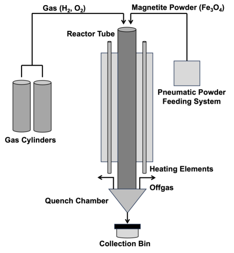
The CRN study presented in this work focuses on the laboratory scale flash reactor. A schematic of the apparatus is shown in Fig. 2. The magnetite powder is fed into the 213 cm long reactor tube of 19.5 cm width by a pneumatic feed system along with the gaseous fuel/oxidizer mixture. Electrical heating is provided by heating elements placed in a furnace around the reactor. Reduced samples are collected in a collection bin after quenching the hot flue gas to reduce the amount of particle loss in the flue gas. The degree of reduction is then determined by inductively coupled plasma mass spectroscopy. During the experiments, the particle residence times, the amount of remaining reducing gases and the flame configuration were varied and their effect on the degree of reduction was studied.

Figure 2: Simplified schematic of the laboratory flash reactor for magnetite reduction, adapted from [21].

In addition to the experimental studies, a three-dimensional Computational Fluid Dynamics (CFD) simulation of the laboratory flash reactor has been performed. The gas phase is modeled in an Eulerian framework, while a Lagrangian description is used to describe the particle phase within a Reynolds Averaged Navier Stokes (RANS) simulation. The simulation results are validated with the experiments and provide useful details on the flow and temperature fields inside the reactor. More information on the experimental and numerical studies is available in [21].

In the present study, the results obtained for the experiments with hydrogen as the only reducing agent have been used for calibration of a CRN model. Sohn and co-workers have found hydrogen to be the driving species for reduction even if carbon-monoxide is present, and testing the calibration is easier with a simpler configuration, too. Out of the various experimental operating conditions reported by Sohn, those with the same flame configuration (HOH, see [21]) and powder-feeding mode (side slots) have been chosen for the present study to reduce the number of variable parameters in a first modeling attempt. Table 3 reports the chosen selection of operating points with respect to gas and particle mass flows along the respective measured reduction degrees.

Table 3: Operation points selected from the experimental studies by Sohn [21] with the relevant operating conditions and experimentally obtained reduction degrees. OP R is not from the Sohn study such that there is no validation data available from experiment or CFD, and has been introduced for testing consistency between the modeling regimes that will be introduced in Section 5.3. The particles always are fed into the reactor by a $\text{N}_{2}$ flow of $2.8\text{\,}\mathrm{L}\text{\,}{\mathrm{min}}^{-1}$.

Operation Point	$\text{H}_{2}$ flow (l/min)	$\text{O}_{2}$ flow (l/min)	$\text{Fe}_{3}\text{O}_{4}$ flow (g/min)	Reduction Degree (%)
A	15.3	2.16	1.9	82
B	15.3	2.36	1.7	76
C	15.3	2.48	2.0	70
D	15.3	2.50	1.9	70
E	15.3	2.72	2.1	57
F	20.0	2.20	2.2	96
G	20.0	2.96	1.8	84
H	20.0	2.96	2.2	80
I	20.0	3.22	1.9	80
J	20.0	3.70	2.0	63
K	40.0	4.32	2.2	92
L	40.0	6.40	2.1	77
M	60.0	9.65	1.9	74
N	60.0	9.65	2.2	74
O	60.0	10.65	2.3	72
P	60.0	11.20	2.0	64
Q	60.0	12.20	2.0	49
R	20.0	3.50	2.0	-

4.1 Kinetic mechanism

As mentioned before, Sohn et al. have developed kinetic mechanisms for the reduction of hematite and magnetite powders in different reducing atmospheres [22, 24, 25, 21].

For magnetite reduction with temperatures up to $1623\text{\,}\mathrm{K}$, a global rate expression has been obtained for the reduction degree, which is a dimensionless measure for the progress of the reduction given by [21]:

$$X=\frac{m_{\textrm{i}}-m_{\textrm{t}}}{m_{\textrm{i}}Y_{\textrm{O,sol,i}}},$$ (55)

where $X$ is the reduction degree defined on $\left[0,1\right]$, $m_{\textrm{i}}$ is the initial solid mass of the experimental sample (not to be confused with a statistical sample in the present calibration context) and $m_{\textrm{t}}$ the sample mass after reduction and $Y_{\textrm{O,sol,i}}$ is the mass fraction of oxide bounded in the sample before reduction, where the mass fraction is with respect to the total solid sample mass, not to be confused with the general mass fractions stated in the CRN context, e.g. Equations (1) and (2).

The global rate equation for the reduction degree reads the following initial value problem [21]:

$$\frac{dX}{dt}=a\cdot\exp\left[\frac{-E_{\textrm{A}}}{RT}\right]\cdot\left[p_{\textrm{H}_{2}}-\frac{p_{\textrm{H}_{2}\textrm{O}}}{K}\right]\cdot(1-X),$$ (56)

$$X(0)=X_{0},$$ (57)

where $p_{\textrm{H}_{2}}$ and $p_{\textrm{H}_{2}\textrm{O}}$ are the hydrogen and steam partial pressures, measured in atm, $K$ is the equilibrium constant, which depends on the temperature and has been determined experimentally [24], $a$ is an Arrhenius-type pre-factor, and $E_{\textrm{A}}$ is an activation energy. The experimentally determined values provided by Sohn are $a=1.23\cdot 10^{7}\frac{1}{\textrm{atm}}$ and $E_{\textrm{A}}=$196\,000\text{\,}\mathrm{J}\text{\,}{\mathrm{mol}}^{-1}$$. It holds $X_{0}=0$ throughout this work.

This global equation gives no information about the fractions of different iron or iron oxide phases during reduction, and according to [22] these are in general not known during experiments. For the numerical CRN solution in NetSMOKE, Equation (57) are transformed to a set of species equations, including magnetite and pure iron, however, without changing the global behavior for the reduction degree and gas species as given in (57). Equation (55) has accordingly been transformed to

$$X=1-\frac{Y_{\text{Fe}_{3}\text{O}_{4}}}{Y_{\text{Fe}_{3}\text{O}_{4},{\text{in}}}},$$ (58)

where $Y_{\text{Fe}_{3}\text{O}_{4}}$ and $Y_{\text{Fe}_{3}\text{O}_{4},{\text{in}}}$ are the current and initial mass fractions of magnetite, now with the mass fractions being relative to the total mass, including gas species. These are the mass fractions that are obtained from the NetSMOKE program. The reduction degree and potentially the gas species, are the only quantity of interest in the given case, and Equation (58) has been used to obtain the reduction degree from the mass fractions computed with NetSMOKE.

Furthermore, the partial oxidation of hydrogen has not been explicitly modeled in the present study; it has been assumed that all oxygen is consumed so fast that this does not have any (chemical) influence on the reduction process. This has been motivated by CFD results for the species distribution in the reactor presented in [21]. Contrarily, the influence of the flame on the temperature distribution in the reactor has an important role and is investigated in Section 5.

For CRN solution, it has further been assumed that the solid phase is carried at the same velocity as the gas phase, which is only an approximation, and might contribute to the model error of the applied CRN models; see Sections 2.2 and  5.

4.2 Design space

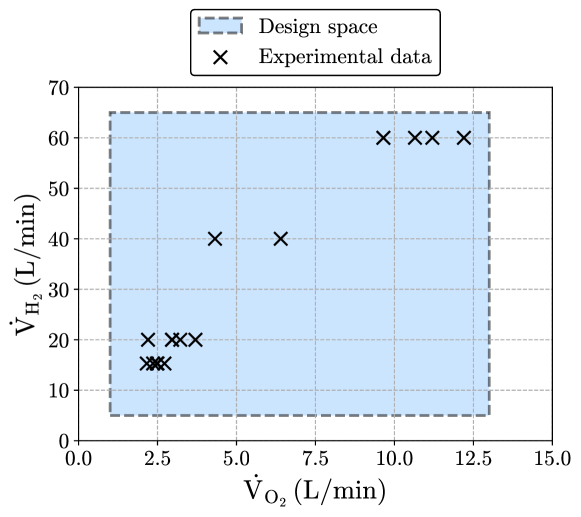
The design space defines the set of operating conditions on which a valid CRN model shall be calibrated. For the laboratory reactor considered in the present work, the relevant operating conditions are the mass flow of magnetite provided to the reactor as well as the hydrogen and oxygen volumetric flows. Moreover, for the present case it is assumed that the hydrogen and oxygen flows have the biggest influence on the CRN model itself, which will be extensively discussed in Section 5. In Figure 3, a projection of the full design space onto the $\dot{V}_{\text{H}_{2}}$-$\dot{V}_{\text{O}_{2}}$-plane is exemplified. However, the exact bounds of the design space are difficult to define for the present case, as there is a correlation between the hydrogen and the oxygen flow for those operation points belonging to the experimental data set. This correlation can be understood since both, too elevated and too low oxygen flows compared to the hydrogen flow would be problematic. If the ratio of oxygen flow to hydrogen flow is too high, there will be no hydrogen left for the actual reduction of magnetite after the partial combustion. If it is too low, the flame will probably not stabilize. The exact definition of the design space for an application case where the available data is non-uniformly spread will be revisited in future work. The focus of the present work is on the actual development of CRN models being valid for, at least, many operation points at once.

Figure 3: Exemplified subset of the design space of operating conditions or the given test case. A valid CRN model shall be calibrated on the full design space. However, for the present case, the exact definition of the design space is difficult, for details it is referred to the text.

5 Results

In the following section, the results of the present study are presented and discussed. This includes the construction of a CRN model to describe the laboratory reactor by Sohn [21] for various operating conditions, preparatory studies for enhancing the model and finally the calibration of the identified sensitive model parameters. The role of the different types of uncertainty in the present case will also be discussed. An overall discussion on the results and the scope of this study in relation to the objectives of this work follows afterwards in Section 6.

5.1 Set up of a CRN model for the lab reactor

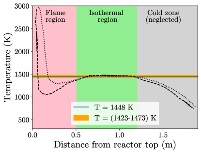
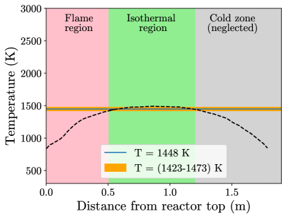
In the present section, a CRN model is set up, which models the lab reactor by Sohn et al. [21] presented in Section 4. The secondary data available in the literature [21, 28, 29, 26, 27, 23], which consists of experimental and CFD data, is used for the development of a CRN model. Hereby, the temperature distribution and flow structure are of particular importance in order to account for the reaction kinetics and residence time. In Figures 4(a) and 4(b), the simulated temperature profile at the reactor center line, and the measured temperature profile at the reactor wall for different operating conditions, as presented in [21], are shown. Sohn and co-workers describe an isothermal temperature region of approximately $70\text{\,}\mathrm{cm}$ length in the middle of the reactor, seen in axial direction, that is approximately constant for all operating conditions and throughout the radial direction of the reactor. This can also be seen in Figures 4(a) and 4(b) and according to Sohn the temperature is $1448\pm$$25\text{\,}\mathrm{K}$. This zone is denoted as an isothermal reaction zone. It is located between approximately $50\text{\,}\mathrm{cm}$ and $120\text{\,}\mathrm{cm}$ away from the top line of the reactor.

Above the isothermal reaction zone, the flame for partial oxidation of hydrogen is situated. Therefore, this region will be referred to as the flame region in the following. As can be seen in Figure 4(a), there is a huge temperature gradient at the center line, where the hottest part of the flame is located. The exact temperature profile, including the spatial extent of the flame, strongly depends on the operating condition. In total numbers, temperatures between approximately $1100\text{\,}\mathrm{K}$ and $3100\text{\,}\mathrm{K}$ are reached.

At the reactor walls, a different behavior can be observed, as can be seen in Figure 4(b). There, an approximately linear increase of temperature, starting from $800\text{\,}\mathrm{K}$, and finally reaching the isothermal temperature of $1448\text{\,}\mathrm{K}$, is visible. From this data, it can be concluded that the exact spatial temperature in the flame region is strongly dependent on the operating condition and in general not known without access to primary data. In addition, Sohn reports a turbulent zone in the upper part of the reactor, while there is laminar flow in the lower part (see [21], p. 164). Thus, the particles will be dispersed in the flame region, and it is not clear in how far they pass the hottest regions of the flame while being inserted through the side slots (see Section 4).

This is why in a first CRN modeling attempt, this region is modeled as one compartment, whose temperature is treated as a (highly) uncertain model parameter. The isothermal region is modeled as another compartment of the CRN. As there is a turbulent zone in the upper part of the reactor, the flame region is modeled by a perfectly stirred reactor (PSR) modeling block, whereas the isothermal zone is modeled by a plug flow reactor (PFR) modeling block as laminar flow is dominant further down the reactor. From the data available, it is not entirely clear if the transition from turbulent to laminar flow regimes is exactly located at $50\text{\,}\mathrm{cm}$ from the top of the reactor, where the boundary between flame and isothermal zone has been defined, but this assumption is at least not unreasonable (cf. [21], p. 164).

Finally, a strong decrease in temperature both at the reactor center line and near the walls is observable further down the reactor, below the isothermal region, in Figures 4(a) and 4(b), and Sohn also assumes that there is no significant reaction ongoing in that region [21]. Therefore, this region is neglected in the CRN model developed here.

All together, the proposed generic CRN model is depicted in Figure 5, consisting of a PSR and a PFR in series, where the PSR temperature is not known a priori and will depend on the operating conditions, as will be seen later on, and the PFR temperature is $1423\text{\,}\mathrm{K}$ .

It has to be noted that this is an extremely simple CRN model, even in the scope of CRN models being strongly reduced models compared to CFD or experiments. However, as has already been mentioned above, with the given data it is hardly possible to construct a more complex model without having the necessary information at hand. Next, and maybe more important, with the objective of this work being the calibration of a CRN on the full design space of operating conditions, the extent, to which details that are strongly dependent on the operating conditions can be modeled in a meaningful way, is limited. Finally, the present laboratory reactor, other than directly inside the flame, exhibits rather simple fluid dynamics and temperature profiles compared to other chemical reactors, and through employing uncertainty quantification, it will be possible to evaluate the quality of this simple model afterwards.

Before calibration of the CRN model, it is tested for single operation points, and results are reported in the following section. This serves as a partial validation of the model and a preparatory study for later calibration.

((a)) Approximate temperature profile at the reactor center line obtained in the CFD simulations by Sohn et al., for different operating conditions, adapted from [21].

((b)) Approximate temperature profile at the reactor wall obtained in the experiments by Sohn et al., adapted from [21].

Figure 5: Simple CRN for modeling the lab reactor, consisting of a perfectly stirred reactor (PSR) for modeling the turbulent flame zone and a plug flow reactor (PFR) for modeling the laminar isothermal zone of the reactor.

5.2 Calibration of the PSR temperature for single operation points

In order to evaluate in how far a CRN model could be calibrated on the full design space, a preparatory study has been conducted. This also serves as a partial validation of the CRN model constructed in Section 5.1, as will be seen below.

For every operation point considered here (see Table 3), a classical calibration of the PSR temperature, which is the only undetermined parameter in the present CRN model, has been conducted. Classical here means that no model and no data error has been considered during the calibration. When only single operation points are used for the calibration, the model error concept would not work anyway and objective of the preparatory one-to-one calibration presented here only is to enable an estimate on how well the CRN model works and to examine how it could be globally calibrated. Note that throughout this work, the objective function of the calibration is always the reduction degree obtained during the flash ironmaking process.

For convenience, the workflow described in Section 3.3 has been used for the calibration, with 0-th order expansions, as no model error has been included. Surrogates have been trained within the temperature range of the uniform priors, which are $1100\text{\,}\mathrm{K}$ to $1400\text{\,}\mathrm{K}$ for OP A - E and $1300\text{\,}\mathrm{K}$ to $1600\text{\,}\mathrm{K}$ for OP F - Q. The training and prior range for the first five operation points has been reduced to lower temperatures after a first calibration attempt has revealed that temperatures are rather located in that region.

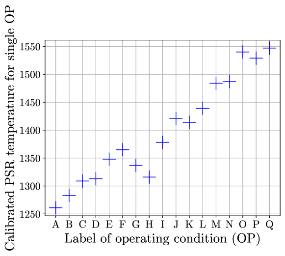
In Figure 6, the results of the classical calibration for each operation point are shown. Please note that there is no link to any physical variable in that plot, so no functional temperature model can be deduced from that representation. This will be achieved by connecting the data to the respective operating conditions in a later step.

However, what can be learned from Figure 6 is the following. Firstly, the calibrated temperatures are in a range between $1261\text{\,}\mathrm{K}$ and $1547\text{\,}\mathrm{K}$ and are more or less evenly spread within that range. This leads to the direct conclusion that it will not be possible to calibrate a single PSR temperature on the full design space, and more parameters are needed. Secondly, however, it can be stated that the calibrated temperature values are consistent and in a reasonable order of magnitude. Overall, a global increase of the calibrated temperature, even though not monotonically, is observed for increasing total gas flow rate (see Table 3). This is reasonable as a higher gas flow will lead to a larger flame, which is also reported by Sohn [21]. Next, it is observed that for some operating conditions the PSR temperature is lower as the temperature in the isothermal region, and for some it is higher. In total, the spread is $\pm\approx$200\text{\,}\mathrm{K}$$ around the isothermal temperature of $1448\pm$25\text{\,}\mathrm{K}$$ ($1423\text{\,}\mathrm{K}$ used as PFR temperature, see Section 5.1). Although the exact temperature profiles within the PSR region are not known, the profiles reported in Figures 4(a) and 4(b) indicate that there are regions with both, strongly lower and higher temperatures present in that zone. The calibrated temperature can be seen as an average temperature actually seen by the particles.

Depending on the flame size and power and the flow behavior of the particles, it is possible, that for some operating conditions, particles on average pass regions with lower temperatures in the upper part of the reactor compared to the isothermal zone, and for some operating condition, the temperature acting on the particles is on average higher than the isothermal temperature, due to the strongly elevated temperatures in the flame.

The results also have shown that there actually is a solution for the PSR temperature for every single operation point. This would not have been the case, if the particles would already reach the experimental value of the reduction degree when only travelling through the PFR zone, which would imply that every physically reasonable PSR temperature would lead to overshooting reduction degrees. On the one hand, this shows that the calibration problem is well-posed, and on the other hand this, together with the considerations above, can be seen as a partial validation of the CRN model, as there are no indicators for the model not being usable for the given task.

Figure 6: Calibrated temperatures for each single operation point (see Table 3). Backgrounds and calibration details are given in the text.

5.3 Modeling of temperature in the flame region

As has been seen in Section 5.2, it is not possible to calibrate a single PSR temperature for covering the full design space of operating conditions. This holds, even if a model error is considered, as the physical problem is known well enough to know that results mostly are sensitive to temperature, and a range of $\approx$300\text{\,}\mathrm{K}$$ will not lead to meaningful results in terms of reduction degrees.

Therefore, more or different model paramters are needed for accurately modeling the reduction degrees that can be obtained in the lab reactor. One possible approach would be to increase the number of CRN parameters, e.g. the number of modeling blocks, which is usually done in the CRN context if the CRN is not able to capture higher-fidelity results, see e.g. [17]. However, as discussed above, the present problem is different, as it is not the CRN per se, which is not able to model the experimental data for given conditions, but the task is to find a model being valid for many operating conditions at once. This is why the authors propose to model the temperature itself, by the introduction of meta parameters to the CRN model. In order to achieve a suitable temperature model, it has to be investigated how the temperature depends on the operating conditions, that is, the species mass flows provided to the reactor.

It is assumed that the hydrogen and oxygen flow rate are the parameters that have the strongest influence on the average temperature in the flame region.

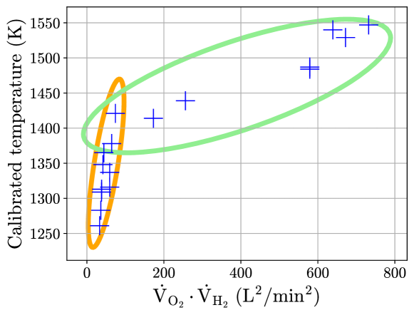
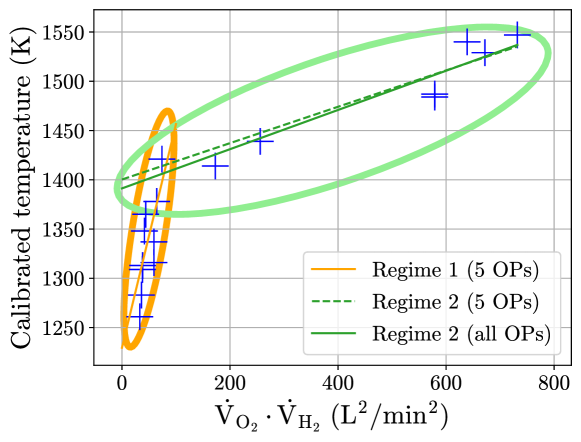
In Figure 7, the calibrated temperatures for single operation points are plotted against the product of volume flows of hydrogen and oxygen. This relationship is investigated under the assumption that the energy released from combustion per time is proportional to the oxygen flow, as all oxygen is consumed in the flame. Furthermore, it is assumed that the flame size is in first order proportional to the total gas volume flow, which is dominated by the hydrogen flow. It is expected that the particles mostly do not pass the most upper flame region due to the gas flow ejected from the burner. Sohn reports that particles fed through the side slot do not melt, whereas particles fed through the burner do [21], which can confirm this assumption. Therefore, it is assumed that the average temperature acting on particles in the flame region increases with increasing flame size. These are of course heuristic arguments and simplified assumptions, and more sophisticated models for the flame temperature could be used instead, but the objective of this work is the development of a framework that can be extended to more general problems, which is why the given approach has been used.

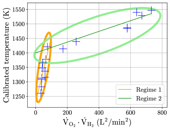
In Figure 7, two overlapping regimes can be identified, which are accordingly marked by colored ellipses in the plot. For both regimes, an approximately linear increase of temperature with different slopes is observed. For this reason, a linear temperature model for each regime is established as follows:

$$T_{1}(\dot{V}_{\textrm{H}_{2}}\cdot\dot{V}_{\textrm{O}_{2}})=k_{1}+m_{1}\cdot\dot{V}_{\textrm{H}_{2}}\cdot\dot{V}_{\textrm{O}_{2}}\ \textrm{{\color[rgb]{1,.5,0}\definecolor[named]{pgfstrokecolor}{rgb}{1,.5,0}(Regime 1)}},$$ (59)

$$T_{2}(\dot{V}_{\textrm{H}_{2}}\cdot\dot{V}_{\textrm{O}_{2}})=k_{2}+m_{2}\cdot\dot{V}_{\textrm{H}_{2}}\cdot\dot{V}_{\textrm{O}_{2}}\ {\textrm{\color[rgb]{0,1,0}\definecolor[named]{pgfstrokecolor}{rgb}{0,1,0}{(Regime 2)}}},$$ (60)

where $T_{1}$ and $T_{2}$ are the PSR temperatures for operating conditions in regimes 1 and 2, respectively, $k_{1}$ and $m_{1}$ are the coefficients of the linear function for regime 1 and $k_{2}$ and $m_{2}$ are the coefficients of the linear function for regime 2. An overview on which operation points belongs to which regime is also given in Table 4. Note, that there are two operation points, which are present in both regimes, making the regimes overlapping. This enables modeling the temperature for operating conditions from the full design space. However, the consistency of the results obtained for operation conditions, whose product of hydrogen and oxygen flow rate is between the values for these two operation points, has to be examined after calibration.

Figure 7: Temperatures calibrated for single operating conditions in Section 5.2, plotted versus the product of volume flows for hydrogen and oxygen as motivated in the text. The ellipses mark the operation conditions assigned to regimes 1 and 2.

Table 4: Overview on the operation points contained in regimes 1 and 2 identified in the present study. "Seen" points are used for calibration of the model parameters, "unseen" points are used for later validation (see Section 5.4).

Regime	operation points
1	A, C, E, G, I (seen)
	B, D, F, H, J (unseen)
2	J, L, N, P, Q (seen)
	I, K, M, O (unseen)

5.4 Calibration and uncertainty quantification for the temperature model

The calibration procedure described in Section 2.4 has been used with the default options given in Table 2 for calibration of $k_{1}$ and $m_{1}$ for regime 1 and $k_{2}$ and $m_{2}$ for regime 2. Further details specific to this calibration are given in Table 5.

Table 5: Calibration options used for the calibration of the temperature model described in Section 5.3, in addition to the default options declared in Table 2.

Parameter	Value
PCE order	1
Surrogate training regions
$k_{1}$	$1000-$1300\text{\,}\mathrm{K}$$
$m_{1}$	$0.5-$8\text{\,}\mathrm{K}\text{\,}{\mathrm{min}}^{2}\text{\,}{\mathrm{L}}^{-2}$$
$k_{2}$	$1200-$1500\text{\,}\mathrm{K}$$
$m_{2}$	$0.001-$0.5\text{\,}\mathrm{K}\text{\,}{\mathrm{min}}^{2}\text{\,}{\mathrm{L}}^{-2}$$

In order to enable later validation of the calibration, only half of the operation points for each regime has been used for calibration, whereas the other half has been used for validation. In regime 1, the points A, C, E, G and I have been used in the calibration, whereas for regime 2 the points J, L, N, P and Q have been used.

In Figure 8, the calibrated linear models for the two regimes are shown together with the temperatures calibrated in Section 5.2. It is important to note that calibration has been done with respect to the experimental reduction degrees, not the calibrated temperatures, although these have been used to motivate the model and determine the priors. This is relevant as the sensitivity of the reduction degree to the PSR temperature is different for different operating conditions.

The calibrated mean values and standard deviations for $k_{1}$, $m_{1}$, $k_{2}$ and $m_{2}$ are given in Table 6.

Table 6: Mean and standard deviation obtained during the calibration of $k_{1}$, $m_{1}$, $k_{2}$ and $m_{2}$.

	Mean	Standard deviation
$k_{1}$	$1229.49\text{\,}\mathrm{K}$	$60.96\text{\,}\mathrm{K}$
$m_{1}$	$2.27\text{\,}\mathrm{K}\text{\,}{\mathrm{min}}^{2}\text{\,}{\mathrm{L}}^{-2}$	$1.24\text{\,}\mathrm{K}\text{\,}{\mathrm{min}}^{2}\text{\,}{\mathrm{L}}^{-2}$
$k_{2}$	$1400.29\text{\,}\mathrm{K}$	$13.83\text{\,}\mathrm{K}$
$m_{2}$	$0.185\text{\,}\mathrm{K}\text{\,}{\mathrm{min}}^{2}\text{\,}{\mathrm{L}}^{-2}$	$0.027\text{\,}\mathrm{K}\text{\,}{\mathrm{min}}^{2}\text{\,}{\mathrm{L}}^{-2}$

Figure 8: Temperatures calibrated for single operating conditions in Section 5.2, plotted versus the product of volume flows for hydrogen and oxygen as motivated in Section 5.3. The ellipses mark the operation conditions assigned to regimes 1 and 2. The linear temperature model for each regime, when mean values for the coefficients $k_{1}$, $m_{1}$, $k_{2}$ and $m_{2}$ obtained in the calibration are applied, is also shown. Note, that calibration has been conducted with respect to the experimental reduction degrees reported in [21] and not directly with respect to the calibrated temperatures for single operating conditions.

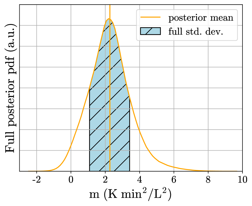
In Figure 9, the full posterior PDFs for the model parameters of regime 1, $k_{1}$ and $m_{1}$ are shown. It is observed that both PDFs are rather broad, with $m_{1}$ even covering negative values. This can be understood from Figure 7, as the temperature increase is only approximately linear and not even monotone. This reveals, that there is potential to further enhance the applied model. However, for these considerations also the results for the reduction degrees have to be taken into account.

((a)) parameter $k_{1}$

((b)) parameter $m_{1}$

Figure 9: Full posterior PDF for the model parameters $k_{1}$ and $m_{1}$ for the temperature model in regime 1.

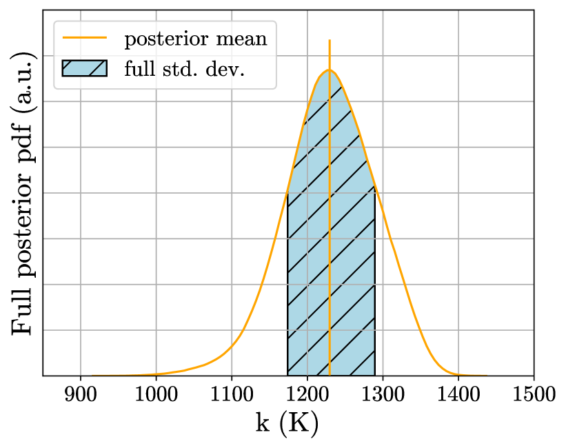
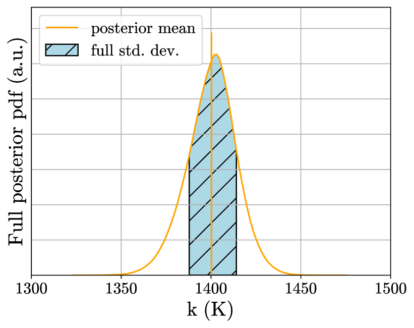
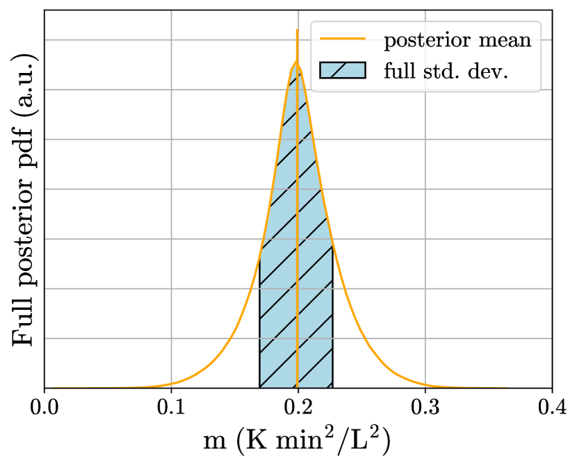
In Figure 10, the full posterior PDFs for parameters $k_{2}$ and $m_{2}$ are presented. The width, i.e. the standard deviation, of these PDF curves is much lower compared to the results for regime 1, so it can be deduced that the model error is lower and the linear approach works better for regime 2. In the following, the CRN predictions when using the calibration results for the PSR temperature are investigated.

((a)) parameter $k_{2}$

((b)) parameter $m_{2}$

Figure 10: Full posterior PDF for the model parameters $k_{2}$ and $m_{2}$ for the temperature model in regime 2.

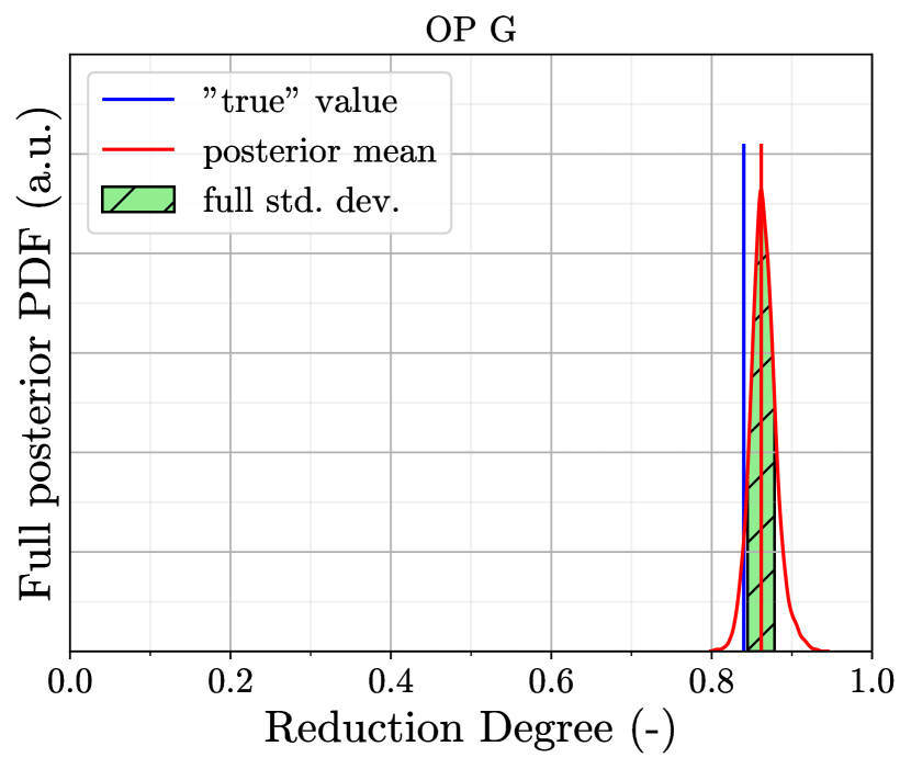
In Figure 11, the full posterior predictions for the reduction degree are shown for two selected operation points from regime 1, which have been used during calibration. An overview of the results for all operation points in regime 1 is given in Appendix 9.1, Figures 18 and 19. It is observed that the PDF curves differ in width and also on how well the mean prediction fits the experimental value. The same is observed for a selection of operation points from regime 2, which have been seen by the calibration, as shown in Figure 13. However, for the operation points of regime 2, the width of the curves is significantly lower than for regime 1, which has already been observed for the model parameters. As the ABC method has been used for likelihood evaluation (see Section 2.4.3), it is expected that the deviation between the mean prediction and the experimental value is on average in the order of the standard deviation, at least for samples of the parameter vector $\bm{\tilde{\alpha}}$ with a high posterior value. In Table 9, the experimental reduction degrees reported by Sohn [21], the mean calibrated values, deviation between the mean prediction and experimental value as well as twice the standard deviation, as width of the $1\sigma$-interval around the mean, are listed for all operation points used in regime 1. For the deviation and (twice) the standard deviation, also average values for all points, and the points seen during calibration, are given, respectively. It is observed that the average (single) standard deviation is approximately the average deviation for the seen points from regime 1. Also for regime 2, the average standard deviation of the seen points fits quite well to the average deviation between mean predictions and experimental values, with the average standard deviation being even a bit higher than the averaged deviation .

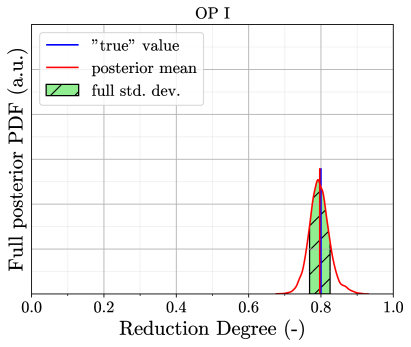
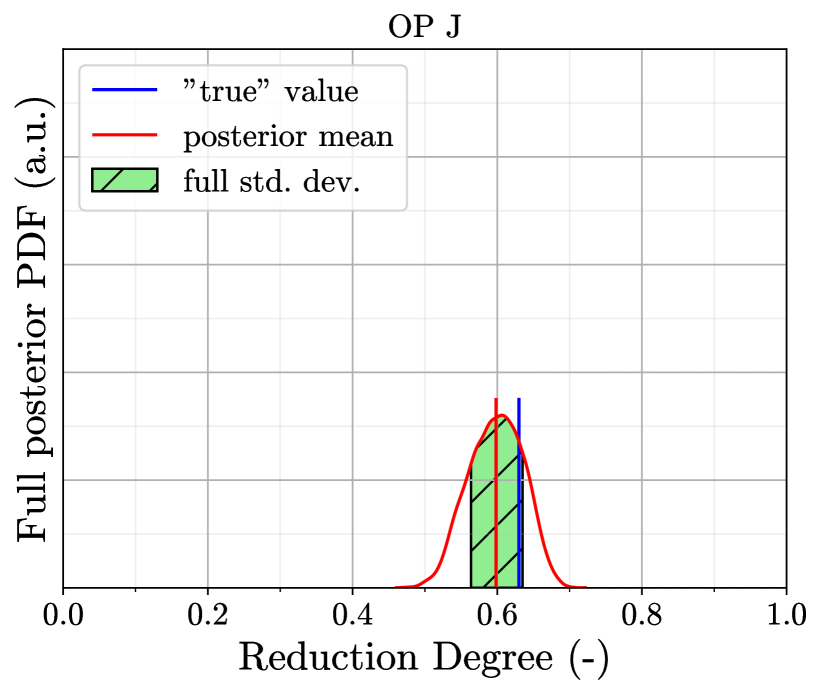
In Figures 12 and 14, a selection of the unseen operation points for regime 1 and 2, respectively, are shown, with all the results being presented in Appendix 9.1.

A further analysis can be conducted with the help of Tables 9 and 10 given in Appendix 9.1. For regime 1, the average deviation between the mean prediction of the reduction degree and the experimental value is 0.0341, with the maximum deviation being 0.046 for operation points E and H. Regarding that a simple CRN model has been used together with a linear temperature model, the predictive capacity of the model is quite good. For regime 2, even lower deviations of on average 0.0224 with a maximum value of 0.039 have been reached. This way, it can be stated that a CRN model of relatively low complexity has been found, which is able to produce acceptable predictions of the reduction degrees obtained in the laboratory reduction reactor developed by Sohn and co-workers [21].

However, also uncertainty quantification is an important part of the prediction, which here means quantification of the model-induced uncertainty, which has been embedded in the model parameters and determined in the calibration along the mean values. The standard deviation of the predictions is an important measure for the quantification of the model error, especially since the ABC method has been used for the likelihood evaluation of samples. For both regimes, the average standard deviation is lower than the average deviation between the mean prediction and the experimental value. For regime 2, this holds especially for the unseen points. This means that the calibrated model underestimates the actual model error. This might be enhanced if more data is used for the calibration, i.e. if all the available operation points are used, which however has the disadvantage that no validation data would be left in that case.

((a)) Full posterior prediction for OP G.

((b)) Full posterior prediction for OP I.

Figure 11: Selection of full posterior predictions for regime 1, with seen operation points, i.e. points used during calibration. The results for all operation points are given in Appendix 9.1.

((a)) Full posterior prediction for OP B.

((b)) Full posterior prediction for OP D.

Figure 12: Selection of full posterior predictions for regime 1, with unseen operation points, i.e. points not used during calibration, but only for validation. The results for all operation points are given in Appendix 9.1.

((a)) Full posterior prediction for OP L.

((b)) Full posterior prediction for OP Q.

Figure 13: Selection of full posterior predictions for regime 2, with seen operation points, i.e. points used during calibration. The results for all operation points are given in Appendix 9.1.

((a)) Full posterior prediction for OP K.

((b)) Full posterior prediction for OP K.

Figure 14: Selection of full posterior predictions for regime 2, with unseen operation points, i.e. points not used during calibration, but only for validation. The results for all operation points are given in Appendix 9.1.

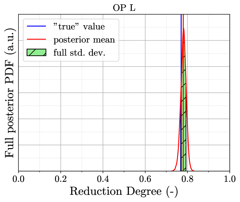
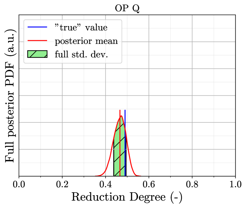
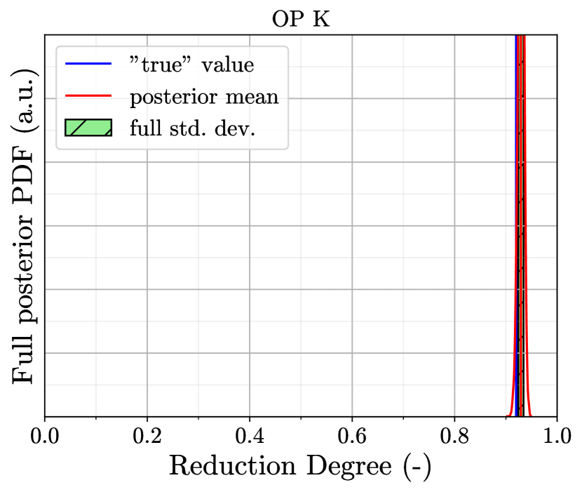
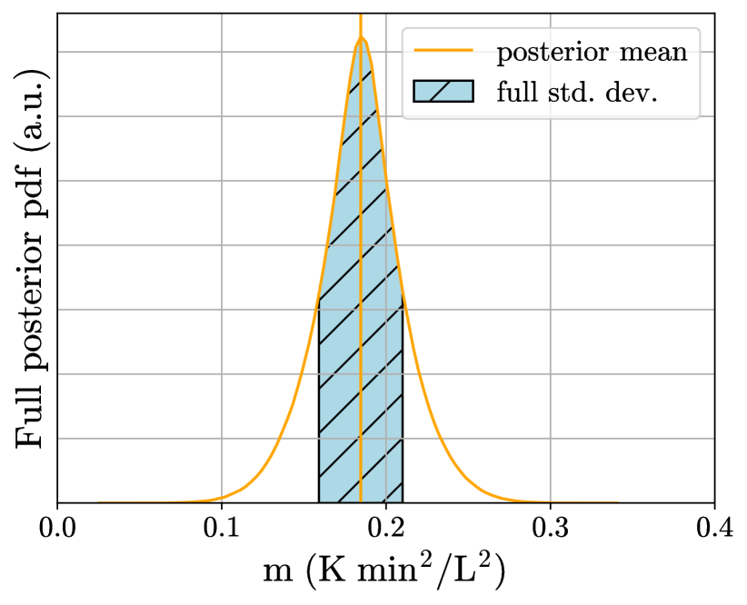
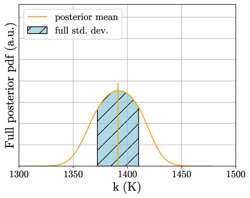
For this reason, it has been investigated in how far using all the available data will enhance the model error quantification. For regime 2, the calibration has been repeated by using all operation points from regime 2 during calibration. In doing so, no prior information from the before calibration has been used. In Figures 15, the full posterior PDFs resulting from the renewed calibration are shown, and the slightly altered linear temperature increase for regime 2 can be seen in Figure 16 together with the temperatures calibrated for single operations points in Section 5.2. The mean and standard deviation of $k_{2}$ and $m_{2}$ are given in Table 7.

((a)) Full posterior prediction for OP K.

((b)) Full posterior prediction for OP K.

Figure 15: Full posterior PDF for the model parameters $k_{2}$ and $m_{2}$ for the temperature model in regime 2, where all operation points of regime 2 have been seen during calibration.

Figure 16: Temperatures calibrated for single operating conditions in Section 5.2, plotted versus the product of volume flows for hydrogen and oxygen as motivated in Section 5.3. The ellipses mark the operation conditions assigned to regimes 1 and 2. The linear temperature model for each regime, when mean values for the coefficients $k_{1}$, $m_{1}$, $k_{2}$ and $m_{2}$ obtained in the calibration are applied, is shown. For regime 2, the results of the renewed calibration with all operation points (solid line) and the previous results, where a selection of operation points has been seen during calibration are shown (dashed line). Note, that calibration has been conducted with respect to the experimental reduction degrees reported in [21] and not directly with respect to the calibrated temperatures for single operating conditions.

Table 7: Mean and standard deviation obtained during the calibration of $k_{2}$ and $m_{2}$ resulting of the calibration with all operation points from regime 2 used.

	Mean	Standard deviation
$k_{2}$	$1391.27\text{\,}\mathrm{K}$	$20.22\text{\,}\mathrm{K}$
$m_{2}$	$0.199\text{\,}\mathrm{K}\text{\,}{\mathrm{min}}^{2}\text{\,}{\mathrm{L}}^{-2}$	$0.031\text{\,}\mathrm{K}\text{\,}{\mathrm{min}}^{2}\text{\,}{\mathrm{L}}^{-2}$

It is observed that especially the width of the posterior PDF of $k_{2}$ has increased, which is also confirmed by an increase of the standard deviation of $k_{2}$. This indicates that the model error actually has increased, the investigation of which has been the objective of the renewed calibration. However, also the results for the prediction of the reduction degree need to be considered.

These results are given in Figures 22 and 23 and Table 11 in Appendix 9.1.4. It is observed that with a value of 0.0211, the average deviation between the experimental value and the mean prediction is even lower than for the calibration with half the points used. At the same time, the average standard deviation has increased, and with a value of 0.022 is now even slightly higher than the average deviation. The increase of standard deviation and its enhanced fitting to the deviation between data and model is expected, as the ABC likelihood has been applied. However, as the prediction capacity of the CRN has not decreased but even increased on average with using more data, it is reasonable to assume that the overall quality of the prediction, including uncertainty quantification, has been increased. In a further step, it should be investigated if a convergence of the model error can be observed when increasing the amount of used data (see Section 7), i.e. the model error not increasing anymore with increasing number of data points used for calibration up from a certain number used. E.g., Sargsyan et al. have reported a model error convergence for a simple test model [20]. Having this information would be beneficial when applying the calibrated model all over the design space, where no validation data is available. A first step in this direction can be the step-wise increase of the number of used data points from five, as hast first been done and described above, to all nine operation points from regime 2. However, for a proper analysis, probably data for more operation points would be needed, which is not or not yet available. A further issue is that no validation data is available to test the results of this renewed calibration with a point not used during the calibration process. Still it can be summarized that especially for regime 2, the simple CRN model together with the modeling approach for the PSR temperature leads to a high prediction quality and a reasonable uncertainty quantification.

Finally, it is to be analysed how meaningful the obtained results are, i.e. how large the uncertainty is relative to the absolute values of the mean prediction and the size of the image set of the CRN model, which here is the interval $\left[0,1\right]$.

As the ABC method has been used for likelihood evaluation, the standard deviation of the posterior curves is on average a measure for the deviation between the mean prediction and the "true" data, i.e. the model error. With an average value of 0.028 for regime 1, and 0.022 for regime 2, the relative model error is small compared to the absolute predictions for the reduction degree. However, it is observed that the standard deviation mostly increases with decreasing mean prediction, meaning that the relative model error is higher for operating conditions leading to lower reduction degrees. This is understandable as the rate of change for the reduction degree, Equation (57), for given operating conditions, decreases with increasing reduction degree, such that also the partial derivative with respect to the temperature is higher for lower values of the reduction degree. For regime 1, the highest relative model error (= standard deviation) for OP J is 9.4%, whereas the lowest for OP F is 0.4%, for regime 2 and all operation points seen in calibration, the highest relative model error is 5.9% for OP J, whereas the lowest value is 0.9%.

Another point to consider is the gain of information obtained from the calibrated CRN model with model error quantification. In the present case, this concerns the region within the interval $\left[0,1\right]$ into which the prediction of the reduction degree can be limited . However, as the posterior prediction PDFs are strongly non-uniform, there is no unique definition of this region available and it also depends on the application, e.g. the design purpose might either be output maximization, or highest robustness.

If using the result, where possible, i.e. computationally tractable, the full PDF information on the prediction should be employed. Other than this, the integrated probability value of a certain interval can be examined, i.e. the one-, two- and three-standard-deviations-intervals ($1\sigma$-, $2\sigma$-, $3\sigma$-intervals) around the mean. For regime 1, this analysis has revealed that on average, the truth value is within the $1\sigma$-interval with a probability of 0.698, in the $2\sigma$-interval with a probability of 0.957 and in a $3\sigma$-interval with a probability of 0.995, with a low scatter among the operation points. For regime 2, it has been found that the truth value is within the $1\sigma$-interval with a probability of 0.64, in the $2\sigma$-interval with a probability of 0.958 and in a $3\sigma$-interval with a probability of 0.999, also with a low scatter among the operation points. Interestingly, these values are quite similar to the well-known values for Gaussian curves.

As has been seen for the single standard deviations, there is strong increase in the width of the $1\sigma$, $2\sigma$ and $3\sigma$-intervals with decreasing mean prediction for the reduction degree. Independently of the exact quantity of interest it can be concluded that there is a clear gain of information through the calibrated CRN model, especially for those operating conditions, for which high reduction degrees are obtained. According to Sohn, these points are the most relevant for the design process, anyway [21]. Quantities of interest could for instance be the mean prediction and its standard deviation, or the lower bound of the prediction. Still, in order to obtain a useful model on the full design space, a refinement of the model such that the model error becomes lower for those operating conditions leading to intermediate reduction degrees, while keeping it low for the high ones, would be beneficial.

Before discussing the obtained results in the light of the overall objective of the present work, there will be further comments on the overlapping of the regimes and the role of the data error.

5.5 Comments on the overlapping of regime 1 and 2

As has been introduced in Section 5.3, the two regimes for the temperature modeling have been defined such that there is an overlap between them within the design space. The operation points I and J (see Table 3) both belong the regime 1 and 2 and the same shall hold for any operation point whose product of hydrogen and oxygen is between those of OP I and J.

For this reason, for these points there are two concurring solutions from regime 1 and 2, whose consistency therefore should be examined. This is why the CRN predictions for a further operation point out of the overlapping region (OP R) have been evaluated. The results for OPs I, J and R for regime 1 and 2 are shown in Figure 17; note that for regime 2 the updated results with all available operation points (except R) seen during calibration has been used. It is observed that for regime 1, the PDF curves are broader than for regime 2, which is a general observation already discussed and not surprising. All mean predictions for regime 2 are still within one standard deviation of the mean result for regime 1, whereas this does not hold the other way around for OP I. For OP J, the mean predictions for regime 1 and two are almost the same and both show are rather high standard deviation of 0.059 and 0.037, respectively. For OP I, the prediction of regime 1 is better than the one of regime 2. For OP R, no such statement on the mean prediction is possible as there is no validation data for this point available.

All together, it can be stated that the result in the overlapping region are not entirely consistent and a redefinition of the boundary between the two regimes should be considered. E.g., it may be possible to define just one operation point as the boundary, which in the present case could be OP J, as it has been seen that at least the predictions are very close to each other for that point. However, in general it is an issue that there is a step in the magnitude of the model error, i.e. the standard deviation and its multiples, between the two regimes. Therefore, the proper definition of the boundary, or, possibly a boundary layer, between the two modeling regimes is an open issue that has to be further investigated for the current application case and for general application cases.

((a)) Regime 1, OP I

((b)) Regime 1, OP J

((c)) Regime 1, OP R

((d)) Regime 2, OP I (All operation points seen during calibration).

((e)) Regime 2, OP J (All operation points seen during calibration).

((f)) Regime 2, OP R (All operation points seen during calibration).

Figure 17: Comparison of the results for regime 1 and 2 for the operation points being present in both regimes.

5.6 Role of the data error

As introduced in Section 2.2, next to the model error, there can be also a data error, which is the deviation between the unknown "truth" and the actual data. Especially in the scope of experiments the data error is an omnipresent concept. There are several ways to account for the data error. There can be information from the experiment, e.g. on the reproducibility of data, but the data error can also be inferred within the calibration procedure, which can lead to a modified result [20].

For the given case, there is only limited information on the data error available to the authors. A data reproducibility of $\pm 2\%$ is reported by Sohn for the comparison between different methods of the evaluation of the reduction degree [21]. Thus, this can be seen as a lower bound for the data error in the given case.

For some of the operation points used (see Table 3), there are also results of CFD simulations available, see [21]. Especially for lower reduction degrees there partially is a strong deviation between CFD and experimental results with the maximal absolute difference for the used operation points being 0.12 for OP J. This leads to the presumption that the overall data error might be higher than $\pm 2\%$.

To summarize, the magnitude of the data error is not known very well for the given case, and further examinations need to be done on that issue in future work.

6 Discussion

As has been introduced in Section 1, the motivation of the present work is the question to which extent chemical reactor networks (CRNs) can be used as a scale bridge within a model hierarchy spanning a huge range of scales, in the context of developing an innovative metal-based energy circular economy. Therefore, CRN models have to be valid on the full design space of operating conditions and not just for those operating conditions, where also data from experiments or computational fluid dynamics simulations exist. Also, the transferability of CRN models among scales is an important point to consider. As CRNs are models of reduced complexity and therefore, reduced accuracy, the quantification of uncertainties rising from the model itself can bee helpful to find an overall model and to know where to improve it.

In the present work, a first step has been achieved in finding and calibrating a CRN model to describe a laboratory reactor developed by Sohn and co-workers [21] on the full design space. This has been achieved by employing a very similar approach for CRN calibration as has been introduced before by Savarese et al. [18], based on the model-to-model-calibration methods developed by Sargsyan et al. [19, 20]. In the present case, the introduction of meta parameters to the CRN model has been shown to be a useful concept for defining a CRN model on a range of operating conditions while keeping an (extremely) simple CRN structure. Also the partitioning of the design space into two regimes has been helpful, since this way it has been possible to use a linear, that is, "first order" model for the parametrization of the PSR temperature. This is especially helpful if the underlying phenomena are not known to a sufficient extent or not enough data is available for a deeper analysis, which is often the case for high-fidelity models that are difficult to evaluate. The simple model has been found to perform relatively good, in terms of how well the prediction approaches the experimental data, regarding that the relative model error is low for most operation points. This holds especially for those operation points, for which elevated reduction degrees are obtained, which are the most relevant ones for the design purpose, see also [21].

One open issue regarding the present case is a lack of data for intermediate values of $\dot{V}_{H_{2}}\cdot\dot{V}_{O_{2}}$ in regime 2, see Figure 7. Therefore, it will be beneficial to enhance the underlying temperature model, which can for example be achieved by explicitly modeling the flame. This could also lead to smaller model errors in the calibrated parameters themselves, especially in regime 1. When comparing the standard deviations of the calibrated parameters to those of the model prediction, it seems that the PSR temperature might not be the most sensitive parameter for the reduction degree. Indeed, it is plausible that the strongest driving force of the reduction is the amount of excess hydrogen, which is also elaborately discussed by Sohn [21]. In future work, sensitivity analysis will be employed to further examine this. Note, that the excess hydrogen is mostly controlled by the operation conditions, i.e. the hydrogen and oxygen flow, which are model inputs to the CRN model, and thus is not a model parameter of the CRN itself.

These points reveal that a generalization of the framework to other, especially more complex cases, will be a challenge for future work. For example, also within the scope of the present research on metal-fueled energy cycles, there are application cases with more complex reactor geometries, chemical reaction mechanisms, and potentially less data available, as the higher the complexity, the more difficult the evaluation of high-fidelity models. Moreover, for these more complex situations, probably there will be a need to apply more advanced methods of uncertainty qunatification, i.e. for efficient sampling. Still, the present work is a first step that will be further extended.

Another important point to make is on scaling. In the present work, the calibration framework has been tested for a laboratory-scale reactor. For being useful in the development of a large-scale application, the modeling approach needs to be transferred to industrial scales. In the case of flash ironmaking, experimental data for several pilot scales and simulation data from pilot to industrial scale reactors are available [21]. Therefore, the model developed for the laboratory reactor will be extended to these scales in future work. However, in the scope of design and optimization problems, it should be considered to incorporate geometry and size as variables themselves, making them accessible to optimization and efficiency analysis along with the other relevant parameters.

7 Conclusion and Outlook

Within the present work, a laboratory reactor for innovative flash ironmaking, for which data is available in the literature [21], has been modeled by a chemical reactor network (CRN). This model has been developed based on secondary data from experiments and computational fluid dynamics simulations from [21] with the objective of creating a valid model on the full design space, while data is only available on a discrete, finite subset. Uncertain parameters have been calibrated along with quantification of uncertainties resulting from the inaccuracy of the model, following an approach suggested by Savarese et al. [18] based on the work by Sargsyan et al. [19, 20]. The long-term objective of this work is using CRN models within large-scale optimization and efficiency analyses, while incorporating information from the nano- to the mesoscale, in the development of large-scale applications, especially in the scope of the current development of a metal-fueled energy circular economy [2, 3].

The next steps include enhancements of the model described in this article, among them it will be investigated how to improve the flame modeling, and possibly alternative approaches for the temperature model. Also, including more CRN model parameters being uncertain, potentially accompanied by sensitivity analysis, will be considered if it shows to be beneficial. Also, there will be further investigation of model error convergence and its stability among the design space and of the role of data errors and their quantification. As discussed in Section 6, upscaling will subsequently be an important step for reaching the long-term objective.

As has also been discussed in Section 6, there will be challenges in the generalization of the approach, especially to more complex test cases. These will be further investigated in future work.

8 Acknowledgements

Funded by the Hessian Ministry of Higher Education, Research, Science and the Arts - cluster project Clean Circles. The authors would like to thank Prof. Tiziano Faravelli and Prof. Alessandro Stagni for the fruitful discussions and advice regarding CRN modeling and for providing the NetSMOKE framework, and Jannik Neumann for the valuable exchange on the integration of technologies for iron oxide reduction.

9 Appendix

9.1 Calibration results

9.1.1 Calibration of PSR temperature for single operation points

In Table 8, the results of the PSR temperature calibration for single operation points are listed.

Table 8: Results of the classical PSR temperature calibration as presented in Section 5.2.

Operation point	Calibrated temperature
A	1261 K
B	1283 K
C	1309 K
D	1313 K
E	1348 K
F	1360 K
G	1337 K
H	1316 K
I	1378 K
J	1421 K
K	1414 K
L	1439 K
M	1484 K
N	1487 K
O	1540 K
P	1529 K
Q	1547 K

9.1.2 Calibration of model parameters for PSR temperature in regime 1

In Figures 18 and 19, the full posterior PDFs of the predictions of the reduction degree obtained from the calibrated CRN model for regime 1 are shown. In Table 9, the experimental reduction degrees reported by Sohn [21] are compared to the predictions of the CRN model developed within the present work, the deviation between the latter two values and width of the $1\sigma$-interval of the prediction, for the operation points of regime 1.

((a)) Full posterior prediction for OP A (seen).

((b)) Full posterior prediction for OP B (unseen).

((c)) Full posterior prediction for OP C (seen).

((d)) Full posterior prediction for OP D (unseen).

((e)) Full posterior prediction for OP E (seen).

((f)) Full posterior prediction for OP F (unseen).

Figure 18: Overview of full posterior predictions for regime 1 and OP A to F.

((a)) Full posterior prediction for OP G (seen).

((b)) Full posterior prediction for OP H (unseen).

((c)) Full posterior prediction for OP I (seen).

((d)) Full posterior prediction for OP J (unseen).

((e)) Full posterior prediction for OP R (unseen, no validation data available).

((f)) Full posterior prediction for OP F, zoomed in, with full y-axis.

Figure 19: Overview of full posterior predictions for regime 1 and OP G-J and R; and for F with a reduced x-axis and full y-axis for better visualization.

Table 9: Overview on the results obtained with the calibrated CRN for regime 1. The average value is only a useful concept for the deviation between the mean prediction and experimental value and the (doubled) standard deviation. ^∗ unseen, no validation data available

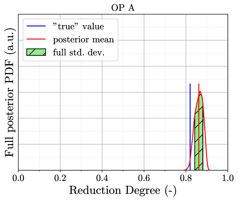
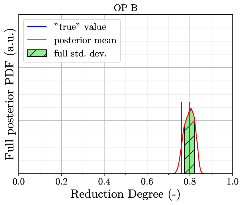
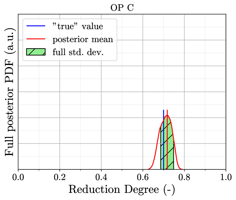
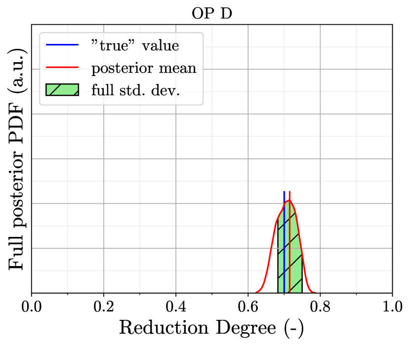
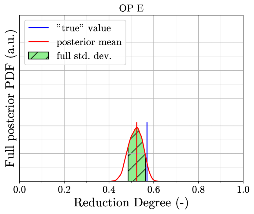
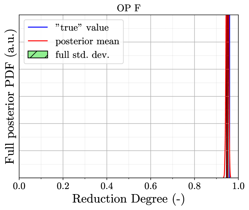
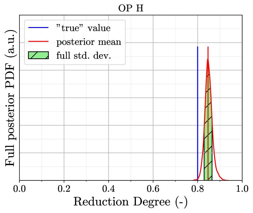
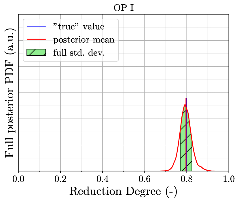
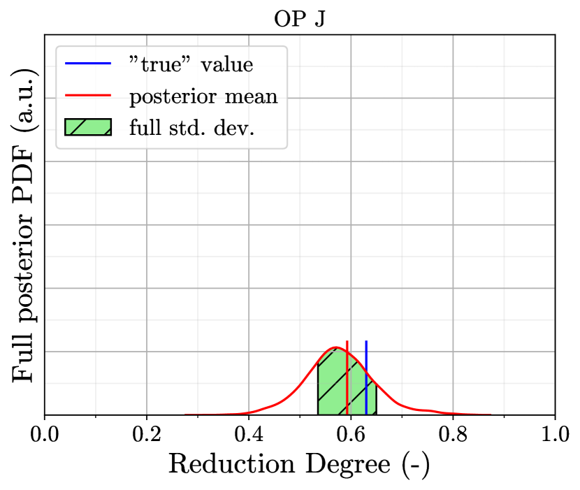
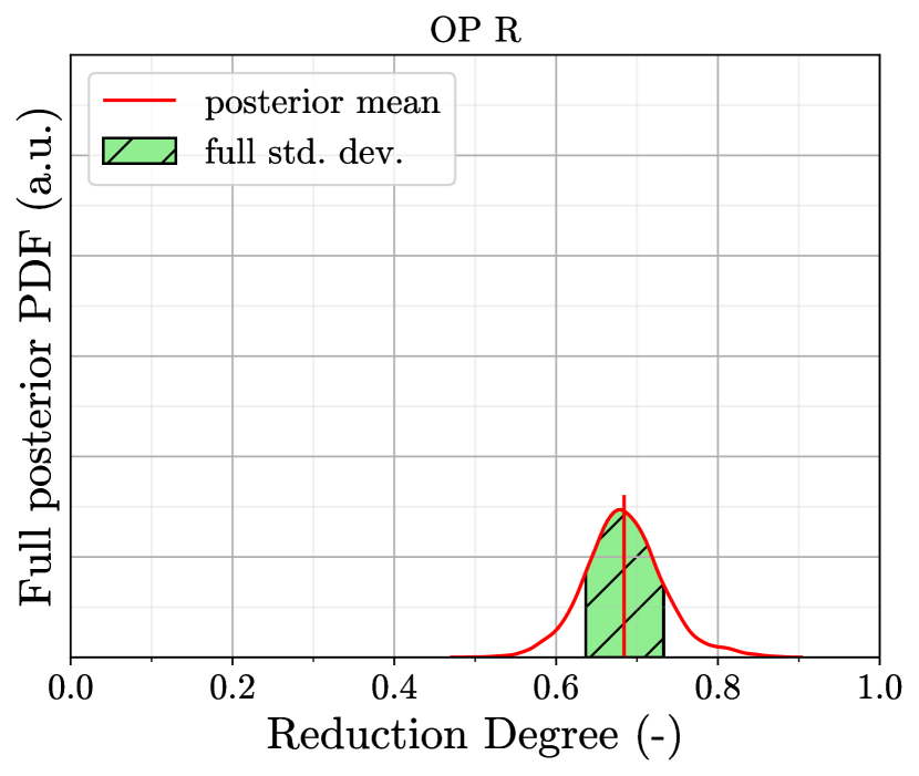
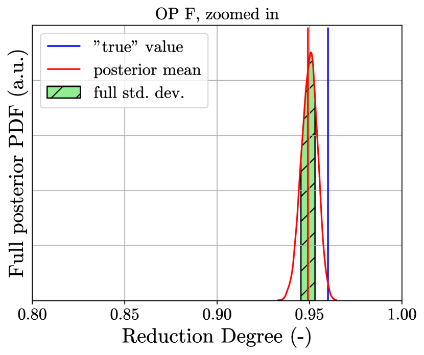
Operation point	Experimental value	Mean prediction	Deviation	$2\cdot$ standard deviation
A (seen)	0.82	0.861	0.041	0.034
B (unseen)	0.76	0.799	0.039	0.049
C (seen)	0.70	0.718	0.018	0.063
D (unseen)	0.70	0.715	0.015	0.067
E (seen)	0.57	0.524	0.046	0.081
F (unseen)	0.96	0.949	0.011	0.008
G (seen)	0.84	0.862	0.022	0.036
H (unseen)	0.80	0.846	0.046	0.038
I (seen)	0.80	0.797	0.003	0.059
J (unseen)	0.63	0.592	0.038	0.118
Average	-	-	0.0279	0.0553
				(= 2$\cdot$ 0.02765)
Average seen points	-	-	0.026	0.0546
				(= 2$\cdot$ 0.0273)
Average unseen points	-	-	0.0298	0.056
				(= 2$\cdot$ 0.028)
R ∗	-	0.684	-	0.099
				(= 2$\cdot$ 0.049)

9.1.3 Calibration of model parameters for PSR temperature in regime 2

In Figures 20 and 21, the full posterior PDFs of the predictions of the reduction degree obtained from the calibrated CRN model for regime 2 are shown, for the first calibration that has been conducted with five seen points, and four left for validation. In Table 10, the experimental reduction degrees reported by Sohn [21] are compared to the predictions of the CRN model developed within the present work, the deviation between the latter two values and width of the $1\sigma$-interval of the prediction, for the operation points of regime 2 for the first calibration.

((a)) Full posterior prediction for OP I (unseen).

((b)) Full posterior prediction for OP J (seen).

((c)) Full posterior prediction for OP K (unseen).

((d)) Full posterior prediction for OP L (seen).

((e)) Full posterior prediction for OP M (unseen).

((f)) Full posterior prediction for OP N (seen).

Figure 20: Overview of full posterior predictions for regime 2 and OP I to N.

((a)) Full posterior prediction for OP O (unseen).

((b)) Full posterior prediction for OP P (seen).

((c)) Full posterior prediction for OP Q (seen).

((d)) Full posterior prediction for OP R (unseen, no validation data available).

((e)) Full posterior prediction for OP K, zoomed in, with full y-axis.

Figure 21: Overview of full posterior predictions for regime 2 and OP O-R; and for K with a reduced x-axis and full y-axis for better visualization.

Table 10: Overview on the results obtained with the calibrated CRN for regime 2. The average value is only a useful concept for the deviation between the mean prediction and experimental value and the (doubled) standard deviation. ^∗ unseen, no validation data available

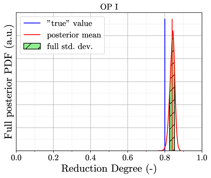
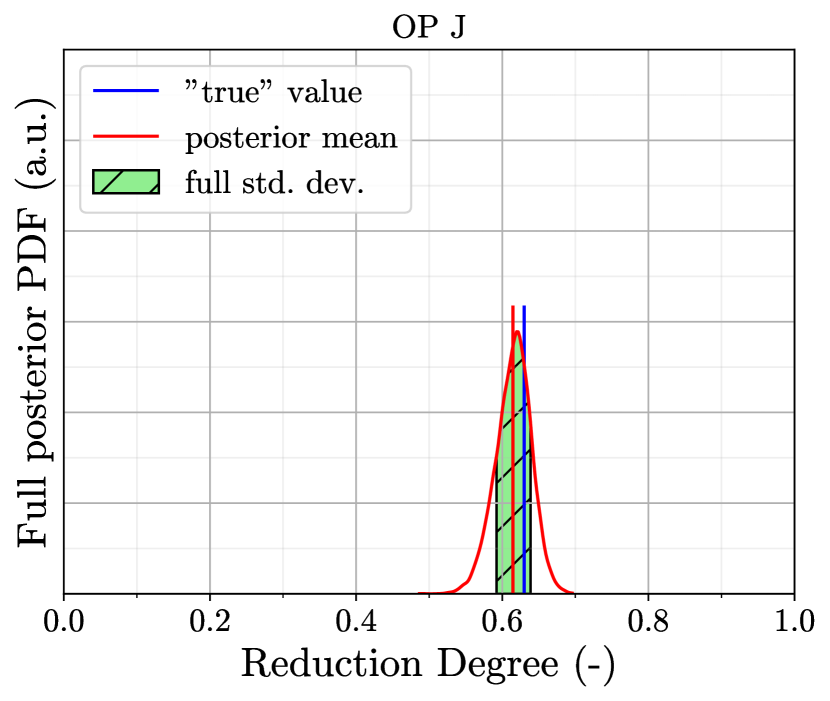
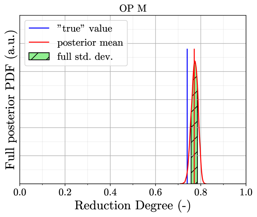
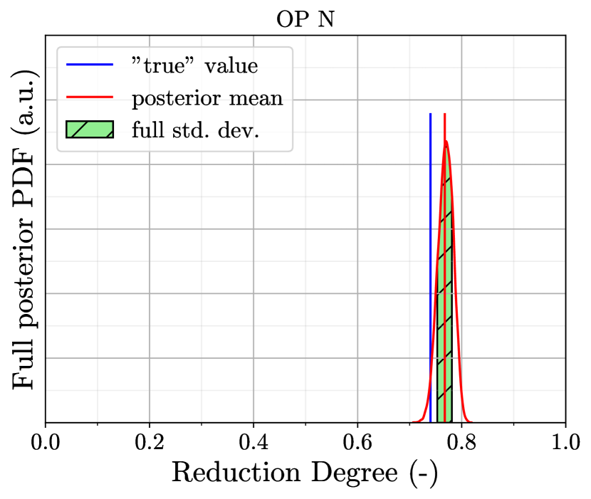
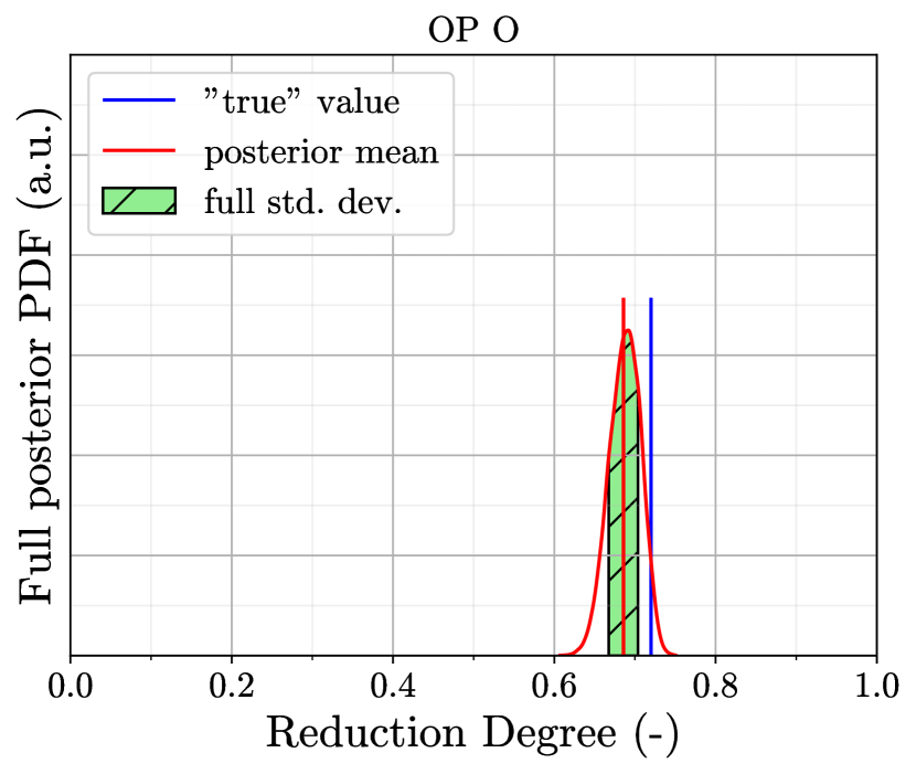
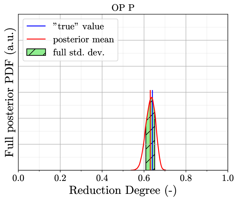
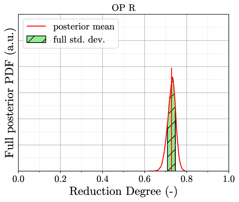
Operation point	Experimental value	Mean prediction	Deviation	$2\cdot$ standard deviation
I (unseen)	0.80	0.839	0.039	0.027
J (seen)	0.63	0.614	0.016	0.046
K (unseen)	0.92	0.929	0.009	0.011
L (seen)	0.77	0.78	0.01	0.026
M (unseen)	0.74	0.771	0.031	0.028
N (seen)	0.74	0.768	0.028	0.028
O (unseen)	0.72	0.686	0.034	0.037
P (seen)	0.64	0.629	0.011	0.043
Q (seen)	0.49	0.466	0.024	0.057
Average	-	-	0.0224	0.0337
				(= 2$\cdot$ 0.01683)
Average seen points	-	-	0.0178	0.04
				(= 2$\cdot$ 0.02)
Average unseen points	-	-	0.0283	0.0258
				(= 2$\cdot$ 0.0129)
R ∗	-	0.728	-	0.040
				(= 2$\cdot$ 0.020)

9.1.4 Calibration of model parameters for PSR temperature in regime 2, with all available operations points used

In Figures 22 and 23, the full posterior PDFs of the predictions of the reduction degree obtained from the calibrated CRN model for regime 2 are shown, for the second calibration that has been conducted with all available operations points seen during calibration. In Table 11, the experimental reduction degrees reported by Sohn [21] are compared to the predictions of the CRN model developed within the present work, the deviation between the latter two values and width of the $1\sigma$-interval of the prediction, for the operation points of regime 2 for the second calibration.

((a)) Full posterior prediction for OP I (unseen).

((b)) Full posterior prediction for OP J (seen).

((c)) Full posterior prediction for OP K (unseen).

((d)) Full posterior prediction for OP L (seen).

((e)) Full posterior prediction for OP M (unseen).

((f)) Full posterior prediction for OP N (seen).

Figure 22: Overview of full posterior predictions for regime 2, where all available operation points of regime 2 have been used for calibration; OP I to N.

((a)) Full posterior prediction for OP O (unseen).

((b)) Full posterior prediction for OP P (seen).

((c)) Full posterior prediction for OP Q (seen).

((d)) Full posterior prediction for OP R (unseen, no validation data available).

((e)) Full posterior prediction for OP K, zoomed in, with full y-axis.

Figure 23: Overview of full posterior predictions for regime 2, where all available operation points of regime 2 have been used for calibration; OP O-R; and K with a reduced x-axis and full y-axis for better visualization.

Table 11: Overview on the results obtained with the calibrated CRN for regime 2, where all available operation points of regime 2 have been used for calibration. The average value is only a useful concept for the deviation between the mean prediction and experimental value and the (doubled) standard deviation. ^∗ unseen, no validation data available

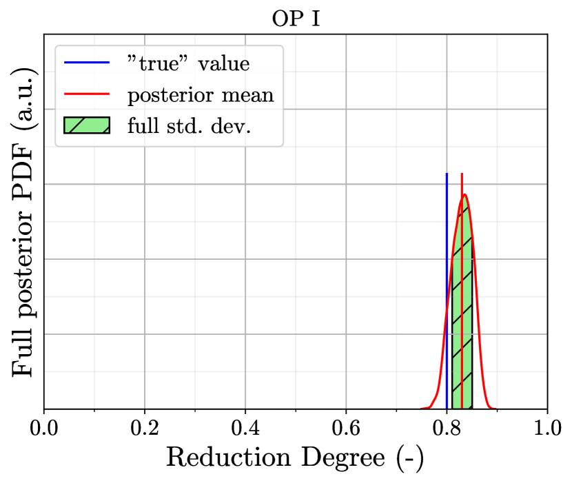
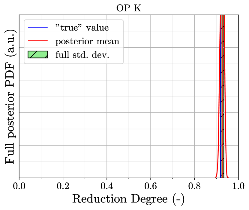
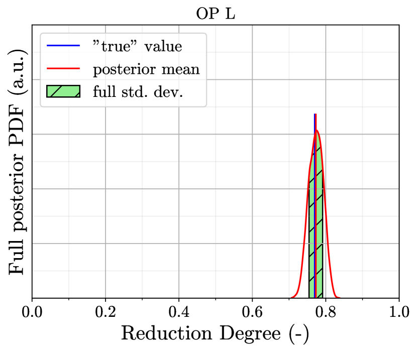
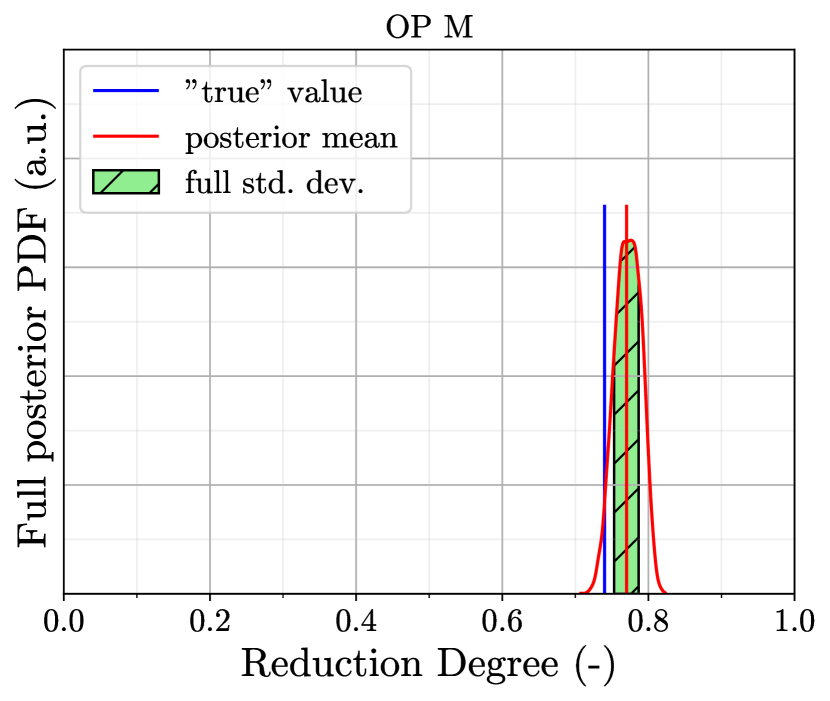
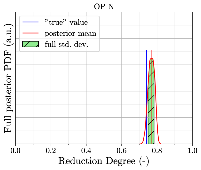
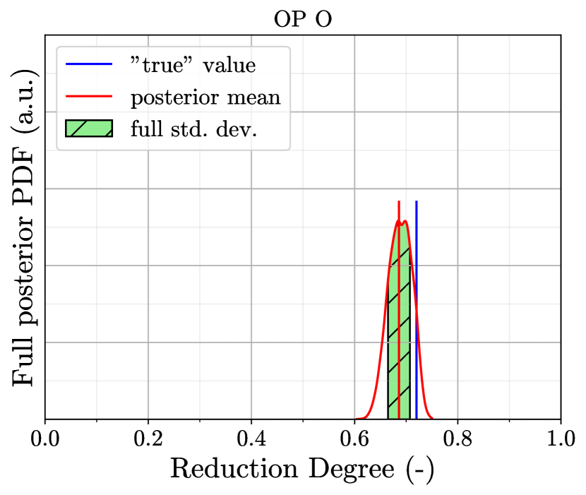
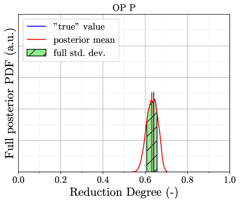
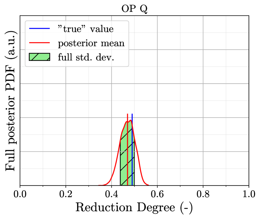
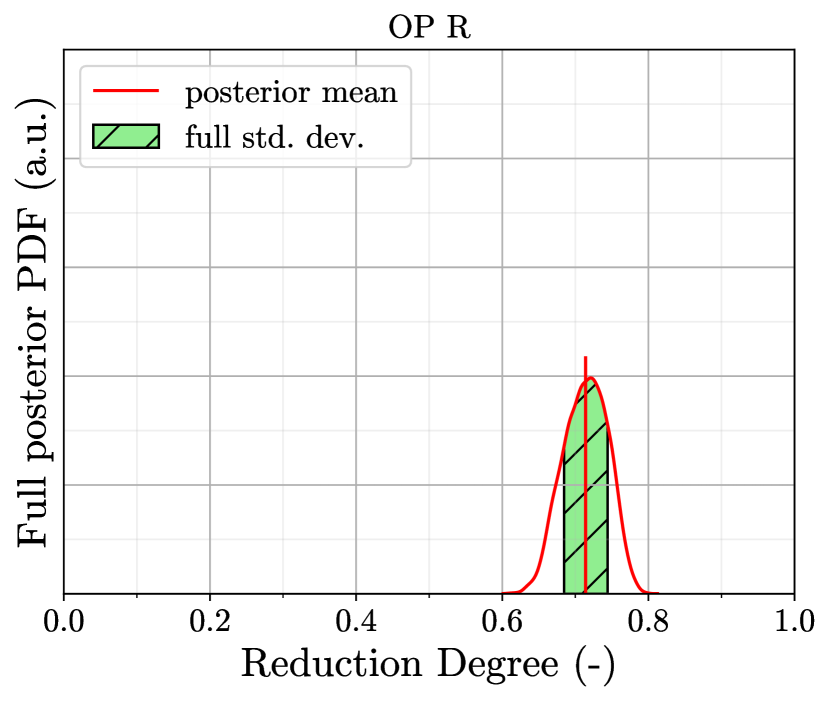
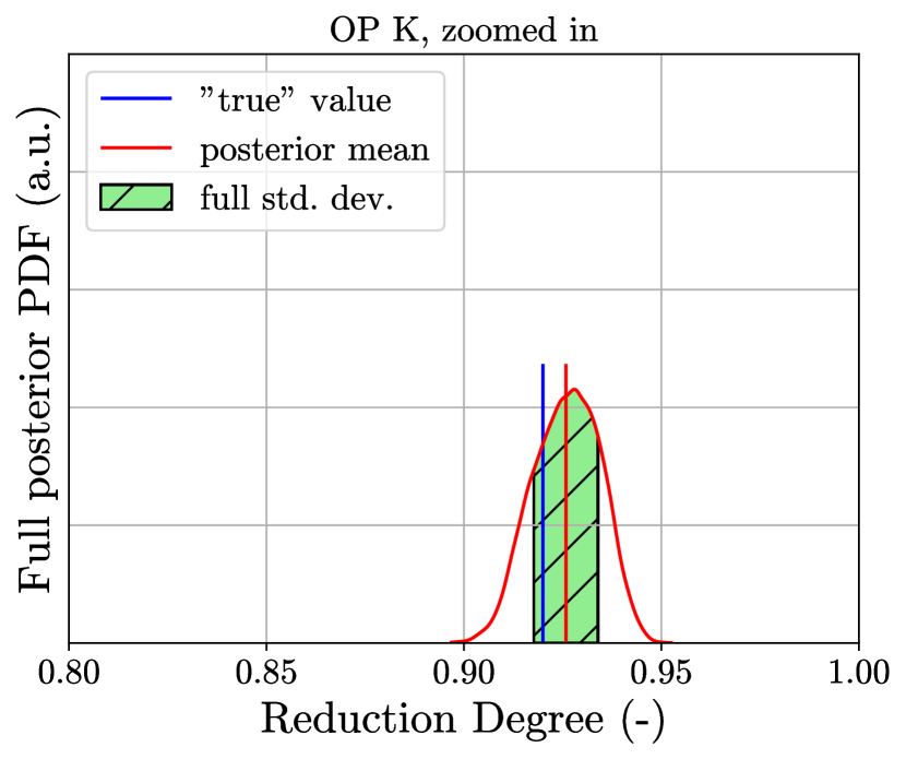
Operation point	Experimental value	Mean prediction	Deviation	$2\cdot$ standard deviation
I (unseen)	0.80	0.83	0.03	0.042
J (seen)	0.63	0.598	0.032	0.074
K (unseen)	0.92	0.926	0.006	0.017
L (seen)	0.77	0.772	0.002	0.040
M (unseen)	0.74	0.77	0.03	0.034
N (seen)	0.74	0.767	0.027	0.034
O (unseen)	0.72	0.686	0.034	0.043
P (seen)	0.64	0.631	0.009	0.049
Q (seen)	0.49	0.47	0.02	0.063
Average	-	-	0.0211	0.044
				(= 2$\cdot$ 0.022)
R ∗	-	0.714	-	0.06
				(= 2$\cdot$ 0.03)

References

- [1] Philippe Julien and Jeffrey M Bergthorson “Enabling the metal fuel economy: green recycling of metal fuels” In Sustainable Energy & Fuels 1.3 Royal Society of Chemistry, 2017, pp. 615–625
- [2] JM Bergthorson et al. “Direct combustion of recyclable metal fuels for zero-carbon heat and power” In Applied Energy 160 Elsevier, 2015, pp. 368–382
- [3] Johannes Janicka et al. “The potential of retrofitting existing coal power plants: A case study for operation with green iron” In Applied Energy 339 Elsevier, 2023, pp. 120950
- [4] Johannes Mich et al. “A comparison of mechanistic models for the combustion of iron microparticles and their application to polydisperse iron-air suspensions” In Combustion and Flame 256, 2023, pp. 112949 DOI: https://doi.org/10.1016/j.combustflame.2023.112949
- [5] Simon Buchheiser et al. “Particle and Phase Analysis of Combusted Iron Particles for Energy Storage and Release” In Materials 16.5, 2023 DOI: 10.3390/ma16052009
- [6] C. Kuhn et al. “Iron as recyclable energy carrier: Feasibility study and kinetic analysis of iron oxide reduction” In Applications in Energy and Combustion Science 12, 2022, pp. 100096 DOI: https://doi.org/10.1016/j.jaecs.2022.100096
- [7] Tao Li et al. “Visualizing particle melting and nanoparticle formation during single iron particle oxidation with multi-parameter optical diagnostics” In Combustion and Flame 245, 2022, pp. 112357 DOI: https://doi.org/10.1016/j.combustflame.2022.112357
- [8] Thomas Krenn et al. “Evaluation of a novel measurement method for the laminar burning speed in laminar lifted iron dust flames” In Fuel 366, 2024, pp. 131266 DOI: https://doi.org/10.1016/j.fuel.2024.131266
- [9] Michal Fedoryk, Björn Stelzner, Stefan Harth and Dimosthenis Trimis “Experimental investigation of the laminar burning velocity of iron-air flames in a tube burner” In Applications in Energy and Combustion Science 13, 2023, pp. 100111 DOI: https://doi.org/10.1016/j.jaecs.2022.100111
- [10] Quentin Fradet, Michalina Kurnatowska and Uwe Riedel “Thermochemical reduction of iron oxide powders with hydrogen: Review of selected thermal analysis studies” In Thermochimica Acta 726, 2023, pp. 179552 DOI: https://doi.org/10.1016/j.tca.2023.179552
- [11] Sören Dübal et al. “Chemical reactor network modeling in the context of solid fuel combustion under oxy-fuel atmospheres” In Fuel 364, 2024, pp. 131096 DOI: https://doi.org/10.1016/j.fuel.2024.131096
- [12] Jannik Neumann et al. “Energy and Exergy Assessment of Renewable Energy Storage using Iron as Energy Carrier” Universitäts-und Landesbibliothek Darmstadt, 2022
- [13] Jannik Neumann et al. “Techno-economic assessment of long-distance supply chains of energy carriers: Comparing hydrogen and iron for carbon-free electricity generation” In Applications in Energy and Combustion Science 14, 2023, pp. 100128 DOI: https://doi.org/10.1016/j.jaecs.2023.100128
- [14] N. Bruch, J. Kemmerzell and M. Knodt “Energy Governance in Europe. A Comparative Analysis of Transition Pathways”, 2023
- [15] Ingrid Ott and Susanne Soretz “Institutional design and spatial (in)equality — The Janus face of economic integration” In European Journal of Political Economy 73, 2022, pp. 102137 DOI: https://doi.org/10.1016/j.ejpoleco.2021.102137
- [16] Friedrich Plank, Johannes Muntschick, Arne Niemann and Michèle Knodt “External Hydrogen Relations of the European Union: Framing Processes in the Public Discourse Towards and within Partner Countries” In Sustainability 15.20, 2023 DOI: 10.3390/su152014757
- [17] Silvio Trespi et al. “Development and Application of an Efficient Chemical Reactor Network Model for Oxy-fuel Combustion” In Energy & Fuels 35.9, 2021, pp. 7121–7132
- [18] Matteo Savarese et al. “Model-to-model Bayesian calibration of a Chemical Reactor Network for pollutant emission predictions of an ammonia-fuelled multistage combustor” In International Journal of Hydrogen Energy 49 Elsevier, 2024, pp. 586–601
- [19] K. Sargsyan, H.. Najm and R. Ghanem “On the Statistical Calibration of Physical Models” In International Journal of Chemical Kinetics 47.4 Wiley, 2015, pp. 246–276 DOI: 10.1002/kin.20906
- [20] Kharchik Sargsyan, Xun Huan and Habib Najm “Embedded Model Error Representation for Bayesian Model Calibration” In International Journal for Uncertainty Quantification, 2019
- [21] Hong Yong Sohn “Flash ironmaking” CRC Press, 2023
- [22] Feng Chen, Yousef Mohassab, Tao Jiang and Hong Yong Sohn “Hydrogen reduction kinetics of hematite concentrate particles relevant to a novel flash ironmaking process” In Metallurgical and Materials Transactions B 46 Springer, 2015, pp. 1133–1145
- [23] Deqiu Fan, Yousef Mohassab and HY Sohn “Computational Fluid Dynamics Simulations of A Laboratory Flash Reactor Relevant to A Novel Ironmaking Process” In CFD Modeling and Simulation in Materials Processing 2016 Wiley Online Library, 2016, pp. 11–18
- [24] Deqiu Fan, Yousef Mohassab, Mohamed Elzohiery and HY Sohn “Analysis of the hydrogen reduction rate of magnetite concentrate particles in a drop tube reactor through CFD modeling” In Metallurgical and Materials Transactions B 47 Springer, 2016, pp. 1669–1680
- [25] De-Qiu Fan, HY Sohn and Mohamed Elzohiery “Analysis of the reduction rate of hematite concentrate particles in the solid state by H 2 or CO in a drop-tube reactor through CFD modeling” In Metallurgical and Materials Transactions B 48 Springer, 2017, pp. 2677–2684
- [26] Amr Abdelghany, De-Qiu Fan, Mohamed Elzohiery and Hong Yong Sohn “Experimental investigation and computational fluid dynamics simulation of a novel flash ironmaking process based on partial combustion of natural gas in a reactor” In steel research international 90.9 Wiley Online Library, 2019, pp. 1900126
- [27] Amr Abdelghany, De-Qiu Fan and HY Sohn “Novel flash ironmaking technology based on iron ore concentrate and partial combustion of natural gas: a CFD study” In Metallurgical and Materials Transactions B 51 Springer, 2020, pp. 2046–2056
- [28] Hong Yong Sohn, De-Qiu Fan and Amr Abdelghany “Design of novel flash ironmaking reactors for greatly reduced energy consumption and CO2 emissions” In Metals 11.2 MDPI, 2021, pp. 332
- [29] Hong Yong Sohn, Mohamed Elzohiery and De-Qiu Fan “Development of the flash ironmaking technology (FIT) for green ironmaking with low energy consumption” In Journal of Energy and Power Technology 3.3 LIDSEN Publishing Inc, 2021, pp. 1–30
- [30] Roger G. Ghanem and Pol D. Spanos “Stochastic Finite Element Method: Response Statistics” In Stochastic Finite Elements: A Spectral Approach New York, NY: Springer New York, 1991, pp. 101–119 DOI: 10.1007/978-1-4612-3094-6_4
- [31] Norbert Wiener “The homogeneous chaos” In American Journal of Mathematics 60.4 JSTOR, 1938, pp. 897–936
- [32] Bert J. Debusschere et al. “Numerical Challenges in the Use of Polynomial Chaos Representations for Stochastic Processes” In SIAM Journal on Scientific Computing 26.2, 2004, pp. 698–719 DOI: 10.1137/S1064827503427741
- [33] Nicholas Metropolis et al. “Equation of state calculations by fast computing machines” In The journal of chemical physics 21.6 American Institute of Physics, 1953, pp. 1087–1092
- [34] W Keith Hastings “Monte Carlo sampling methods using Markov chains and their applications” In Biometrika Oxford University Press, 1970
- [35] Heikki Haario, Eero Saksman and Johanna Tamminen “An adaptive Metropolis algorithm” In Bernoulli JSTOR, 2001, pp. 223–242
- [36] Heikki Haario, Marko Laine, Antonietta Mira and Eero Saksman “DRAM: efficient adaptive MCMC” In Statistics and computing 16 Springer, 2006, pp. 339–354
- [37] A. Cuoci, A. Frassoldati, T. Faravelli and E. Ranzi “OpenSMOKE++: An object-oriented framework for the numerical modeling of reactive systems with detailed kinetic mechanisms” In Computer Physics Communications 192, 2015, pp. 237–264
- [38] Bert Debusschere, Khachik Sargsyan, Cosmin Safta and Kamal Chowdhary “The Uncertainty Quantification Toolkit (UQTk)” In Handbook of Uncertainty Quantification Springer, 2017, pp. 1807–1827 URL: http://www.springer.com/us/book/9783319123844
- [39] Kharchik Sargsyan et al. “UQTk Version 3.1.3 User Manual”, 2023
- [40] G. Rossum “Python tutorial, Technical Report CS-R9526”, 1995
- [41] Charles R. Harris et al. “Array programming with NumPy” In Nature 585.7825 Springer ScienceBusiness Media LLC, 2020, pp. 357–362 DOI: 10.1038/s41586-020-2649-2
- [42] Pauli Virtanen et al. “SciPy 1.0: Fundamental Algorithms for Scientific Computing in Python” In Nature Methods 17, 2020, pp. 261–272 DOI: 10.1038/s41592-019-0686-2
- [43] Tiziano Faravelli et al. “A new procedure for predicting NOx emissions from furnaces” In Computers & Chemical Engineering 25.4-6 Elsevier, 2001, pp. 613–618