Aggregator of Electric Vehicles Bidding in Nordic FCR-D Markets: A Chance-Constrained Program

Abstract

Recently, two new innovative regulations in the Nordic ancillary service markets, the P90 rule and LER classification, were introduced to make the market more attractive for flexible stochastic resources. The regulations respectively relax market requirements related to the security and volume of flexible capacity from such resources. However, this incentivizes aggregators to exploit the rules when bidding flexible capacity. Considering the Nordic ancillary service fcrd, we consider an aggregator with a portfolio of ev using real-life data and present an optimization model that, new to the literature, uses jcc for bidding its flexible capacity while adhering to the new market regulations. Using different bundle sizes within the portfolio and the approximation methods of the jcc, ALSO-X and cvar, we show that a significant synergy effect emerges when aggregating a portfolio of ev, especially when applying ALSO-X which exploits the rules more than cvar. We show that ev owners can earn a significant profit when participating in the aggregator portfolio.

I Introduction

I-A Motivation

A new regulation in the Nordic area has emerged, called the P90 rule, which specifically addresses how fluctuating units such as ev can provide ancillary services by allowing some level of uncertainty in the capacity bid. The P90 rule has the potential to increase liquidity in these markets by lowering barriers to entry for stochastic flexible resources. For example, fcrd has seen soaring prices these past few years, even allowing for a pay-back time of almost one year for a one MW/MWh battery. If fluctuating demand or production, such as grid-connected ev, can participate with their flexibility, the tso can lower their costs for fcrd procurement while ev owners can benefit monetarily. To enable even higher fcrd capacity bids, aggregators can look to exploit the P90 rule and the emerging synergy of pooling ev. In this paper, the synergy effect thus refers to the increase in bidding when aggregating ev. Furthermore, additional requirements have been approved for ler units (such as ev), thus significantly impacting the available flexible capacity for aggregators when bidding for such a portfolio of ev.

The importance of flexibility has increasingly been emphasized in recent years as the tso look into a future with huge growth in both power demand and renewable production with varying and unpredictable characteristics, likely leading to more frequent and severe frequency disturbances in the power grid [1, 2]. Accessing the flexibility of already existing infrastructure, such as flexible demands, can help undertake the green transition and make it more efficient [3]. Demand-side resources constitute a significant amount of unrealized flexibility [4]. However, flexible demand has proved challenging to integrate into ancillary services markets, both due to technical challenges related to their baseline uncertainty [5], but also market and business barriers [6].

In an effort to accommodate and incentivize flexible demand and production to deliver ancillary services, the Nordic tso, including the Danish tso Energinet, are revising their prequalification regulations. In Denmark, Energinet has invented the aforementioned P90 rule for all ancillary services, but also the ler classification scheme for specific frequency services (e.g., fcrd) [7]. They respectively allow for uncertainty related to the reserved capacity bids and lessen the duration requirements for activation which historically have proven to be two significant barriers for market entry of fluctuating units such as ev [8].

Consequently, providing flexibility has rapidly become a hot topic in the electricity-consuming industry. In particular, the fcrd service is experiencing significant traction, with the prequalified capacity more than doubling through 2023 summed for both up and down-regulation [2, 9]. Prices in fcrd up and down-regulation have skyrocketed and since only negligible energy delivery is expected, it serves as an extremely attractive market right now in the Nordics (as opposed to tertiary reserves like mfrr). Notably, companies are rapidly entering this market, but mainly with batteries.

However, there is a big potential for an aggregator to exploit the P90 rule and ler classification to bid grid-connected ev into fcrd which is amplified as a synergy effect upon aggregation. The focus of this paper is indeed to quantify this synergy effect for ev in fcrd by incorporating these new market rules in an optimization framework. To this end, a case study using real-life data of grid-connected ev is used to illustrate their synergy effect for fcrd bidding.

I-B Research questions and our contributions

In this paper, we will specifically be investigating how ev, categorized as ler units, can provide fcrd bids in DK2 by directly incorporating and exploiting the P90 rule from Energinet. The focal point of the paper will be to answer the two following research questions: Given the current market regulation for ancillary services in the Nordic area, (i) how can an aggregator with a portfolio of ev participate in the fcrd market? And, (ii) using real data from ev, how can a potential synergy effect of aggregating ev be exploited for fcrd bidding?

To answer these questions, an optimization approach using jcc to represent the P90 rule has been developed, thus taking risk into account when bidding. In addition, the paper explores and quantifies the significance of the emerging synergy effect when aggregating EVs in bigger portfolios. The synergy effect, in this study, is defined as the added value achieved in terms of increased fcrd capacity bids by bundling ev in bigger portfolios as opposed to individual or smaller clusters while ensuring that the reliability, i.e., security of supply, is kept in accordance with the P90 rule.

I-C Literature review

A vast amount of literature explores the feasibility of demand-side technologies to provide much-needed flexibility to the power grid through engagements in the power balancing market [10, 11, 12, 13]. The references [10, 11] discuss the general concept of demand response and outline market requirements, identified barriers, and the role of aggregators yet, neither of them quantifies the value of participation from an entity perspective. More concretely, [12] looks into the optimal strategy of a centralized battery system participating in multiple ancillary service markets and quantifies the economic viability. The paper proposes an optimization approach but, the battery system is sorely used for providing flexibility thus lacking the uncertainty of another primary usage. Similarly, [13] has been made using ev but here the potential synergy among demand-side assets has not been investigated. Also, the benefits of utilizing demand-side flexibility have been investigated extensively in various other aggregation contexts and market settings such as for energy communities [14, 15], microgrids [16, 15], and prosumer markets [17].

However, neither of the existing literature has been looking at the recent market changes with the P90 which intends to improve the incentive for demand-side flexibility (and production flexibility) participation today. Furthermore, none has specifically tried to explore and exploit the P90 rule within an optimization framework. Thus. although many have looked into the flexibility of ev for ancillary services [13, 18, 19], none with this purpose of maximizing capacity deliverance.

The same goes for fcrd which is a well-examined service to the literature. For example, in [20] the economic potential of utilizing a battery system in, among others, the fcrd market is being quantified. And in [19] which, like this study, has developed a day-ahead bidding strategy via. a stochastic optimization model to assess the value of ev participating in the Nordic FCR markets (includes fcrd). In this study, public charges have been used. However, like the P90 rule, the FCR exclusive ler classification is brand new and has yet to be seen represented in the models representing the market conditions in the literature, up until now.

Various publications have explicitly or indirectly showcased that aggregating fluctuating assets can generate a synergy effect leading to e.g. higher profits as aggregating can help increase the capacity quantity and predictability of available flexibility [21, 11]. For example in [22] it is proven in a bidding context that a coalition of identical flexible assets, here operating on the manual Frequency Restoration Reserve market, always will be incentivized to stay in the coalition as they can increase their respective profits. However, what has not been covered in the literature yet is the potential for utilizing this well-documented synergy effect to progressively exploit the market regulation in an optimization approach, as the P90 rule allows for deliberately taking risks.

The addition of the P90 rule also imposes the possibility of introducing jcc in the mathematical model which is new to the literature. However, in another power system context, they are commonly used when optimizing power flows [23, 24, 25]. Here they are used to incorporate the uncertain penetration coming from renewables. Furthermore, due to the non-convexity induced by chance constraints, the references utilize approximation methods to obtain a tractable optimization problem. Here CVaR is used in [24, 25] whereas both CVaR and ALSO-X can be found applied to a generic chance constraint problem in [26].

With the identified gaps in the literature, this paper uses real ev data, to investigate and quantify the possibility of an aggregator exploiting the synergy effect imposed by aggregation to enable larger bids which have recently been made possible by the introduction of the P90 and ler market regulations.

I-D Paper organization

The rest of the paper is organized as follows. Section II gives an overview of the fcrd market, incumbent regulations of P90 and ler, and the ev data used. Section III describes the simulation setup for the case study, i.e., assumptions, sample generation, and an exact definition of the synergy effect in this context. Section IV introduces the mathematical optimization model incorporating the P90 rule and ler classification as a jcc. This section also introduces two approximations of the jcc, i.e., cvar and ALSO-X. Finally, Section V shows and discusses the results of the case study while Section VI concludes.

II Overview

In this section, we start by introducing the fcrd market with corresponding definitions of the P90 rule and ler units and subsequently provide an appropriate objective function for optimizing fcrd earnings. Second, we illustrate and define the flexibility of a portfolio of ev with respect to the ler regulation using real data.

II-A fcrd

The fcrd market handles large frequency disturbances between 49.5 to 49.9Hz and 50.1 to 50.5Hz and requires a rapid frequency response from fcrd providers (as fast as 2.5 seconds) [7]. Such frequency deviations happen rarely and they typically last for very short durations. Thus, total energy delivery upon fcrd activation is nearly negligible. For example, a 1MW bid of both up and down-regulation for all hours from March 24 (2022) until March 21 (2023) yields 3.25MWh ($\uparrow$) and 4.05MWh ($\downarrow$) activation energy, respectively, equaling only 0,037% ($\uparrow$) and 0,046% ($\downarrow$) of the total bid capacity. Hence, fcrd provision is attractive for an aggregator of ev as activation will not significantly influence their operation schedule or quality of service..

fcrd is an asymmetrical hourly reservation market partitioned into two distinct markets. There is a market for upward regulation and another for downward regulation. The historical hourly reservation prices are shown in Figure 1, showing a market with very volatile and high prices. There are long periods with extreme prices, e.g., fcrd down for most of 2023.

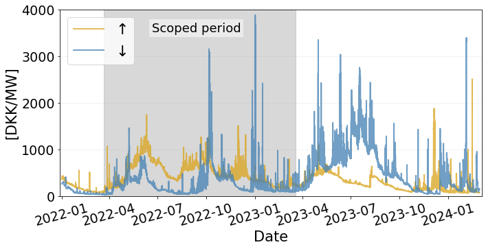
Figure 1: Hourly prices for the fcrd down and up markets from January 1, 2022, to February 29, 2024 [28]. Only the grey area is used in this paper for the case study.

The fcrd auction is composed of an early and late market, both cleared the day before operation, D$-1$, using uniform pricing. As shown in Figure 2, we only consider the early market, where capacity bids, $(c_{h}^{\uparrow},c_{h}^{\downarrow})$, are submitted each for hour $h$ of the following day. These bids are based on available is information, $\omega\in\Omega$, of the ev portfolios flexibility, $F_{m,\omega}$ for every minute, $m$. On the operation day $D$, the activation energy, $A_{m}$, must be delivered according to the realized frequency deviations and the realized flexibility of the ev portfolio, $F_{m}$. Finally, participants are remunerated at fcrd capacity price, $\pi_{h}$, and penalized according to missed activations and excess bids, $(p_{h}^{\uparrow},p_{h}^{\downarrow})$, at price $\lambda_{h}$.

Figure 2: Timeline of fcrd markets in DK2, Denmark. Notice that only the early market is considered here. Optimization variables are denoted with lowercase letters, while uppercase letters are used for parameters. D-1: capacity bids $(c_{h}^{\uparrow},c_{h}^{\downarrow})$ with is flexibility $F_{m,\omega}$. D: Activation energy $A_{m}$ with realized oos flexibility $F_{m}$. D+1: ex-post calculation of penalties $(p_{h}^{\uparrow},p_{h}^{\downarrow})$ at penalty prices $\pi_{h},\lambda_{h}$.

II-B P90 and ler definitions

For conventional units bidding into fcrd, full activation should be possible continually for two hours. For ler units such as ev, the activation duration is relaxed to twenty minutes. However, for ler units, 20% of the submitted bid must be reserved in the opposite direction as follows:

Definition 1 (LER [29])

[…]E.g., If you wish to prequalify 1 MW for fcrd upwards, you must reserve 0.2 MW in the downwards direction for NEM as well as 20 minutes of full fcrd upwards delivery, or 0.33 MWh of energy.

Consequently, ev are considered as ler units for downward regulation, but not for upward regulation purposes (as they can not discharge to the grid). A successful bid thus constitutes an energy reservoir allowing for the downwards activation for 20 minutes continuously, with upwards flexibility being larger than the upwards bid and 20% of the downwards bids, while the downwards flexibility should also be larger than the downwards bid.

Furthermore, Energinet invented the P90 rule specifically for fluctuating resources with stochastic demand or production (such as ev, wind and solar, etc.):

Definition 2 (P90 rule [29])

[…]This means, that the participant’s prognosis, which must be approved by Energinet, evaluates that the probability is 10% that the sold capacity is not available. This entails that there is a 90% chance that the sold capacity or more is available. This is when the prognosis is assumed to be correct. The probability is then also 10%, that the entire sold capacity is not available. If this were to happen, it does not entail that the sold capacity is not available at all, however just that a part of the total capacity is not available. The available part will with a high probability be close to the sold capacity.

Hence, Definition 2 allows aggregators to bid their 10% quantile of forecasted flexibility. Additionally, Energinet has issued a non-pursuable buffer of 5%, meaning aggregators are firstly excluded from the market when there generally is less than an 85% probability that the sold capacity is not available. Definition 2 is evaluated as the average over at least 3 months of data.

II-C ev flexibility

This study has been provided with real-life data of 1,400 ev charge boxes located at residential homes in Denmark. The data is recorded from March 24, 2022, to March 21, 2023. It is assumed that each charge box is only utilized by the same ev. On average, measurements were registered every 2.84 minutes, from which minute resolution consumption profiles have been interpolated for each ev. The ev consumption serves as the baseline for capacity estimates. In Figure 3 the baselines of two different portfolio sizes of ev are illustrated with their maximum charging power for a given hour. Based on that, the available upward $F^{\uparrow}$ and downward $F^{\downarrow}$ flexibility can be derived for each minute. The figure showcases that downward regulation is provided by increasing power consumption while decreasing power consumption delivers upward regulation. Moreover, subject to the baseline consumption, the maximum additional energy that can be consumed by the ev for the upcoming 20 minutes, without saturating the soc or violating the power rate, is found, i.e., its energy flexibility $F^{\text{E}}$. Here, we note that the dataset only contains information regarding the SoC of the specific charging sessions, meaning the aggregator of ev does not know the SoC of the connected vehicle. We assume that every charging session concludes with their being 10% of the total session’s charged energy left on the EV’s battery, [30], which is accessible for deliverance downward flexibility. We simple refer to flexibility as the three-tuple $F=(F^{\uparrow},F^{\downarrow},F^{\text{E}})$.

Figure 3(a) illustrates how a single ev cannot provide any flexibility when it is not connected. Figures 3(b) and 3(c) show the flexibility contained in a portfolio of 1400 ev with and without ler constraints as per Definition 1. In Figure 3(c) the upward flexibility is prioritized to facilitate the downward capacity, as it can enable five times as much capacity by doing so compared to bidding it into the upward market. Therefore, most of it can be seen to be dissolved when compared to Figure 3(c). Moreover, a substantial amount of the downward flexibility is unavailable at the beginning of the hour, as the discrepancy between upward and downward flexibility is too big.

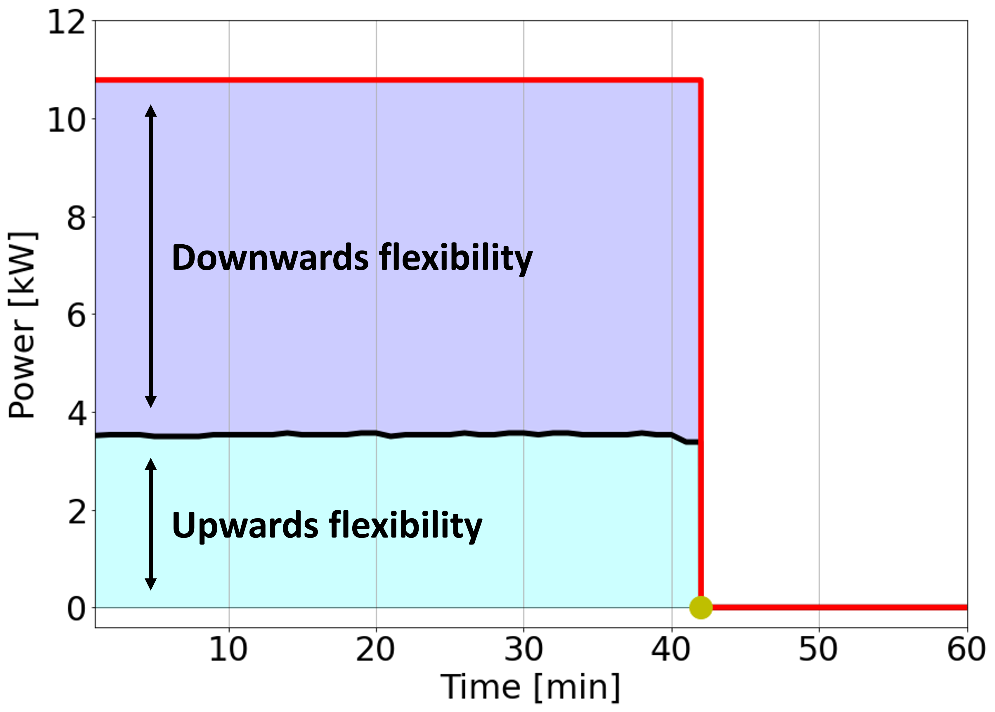
(a) One ev without LER req.

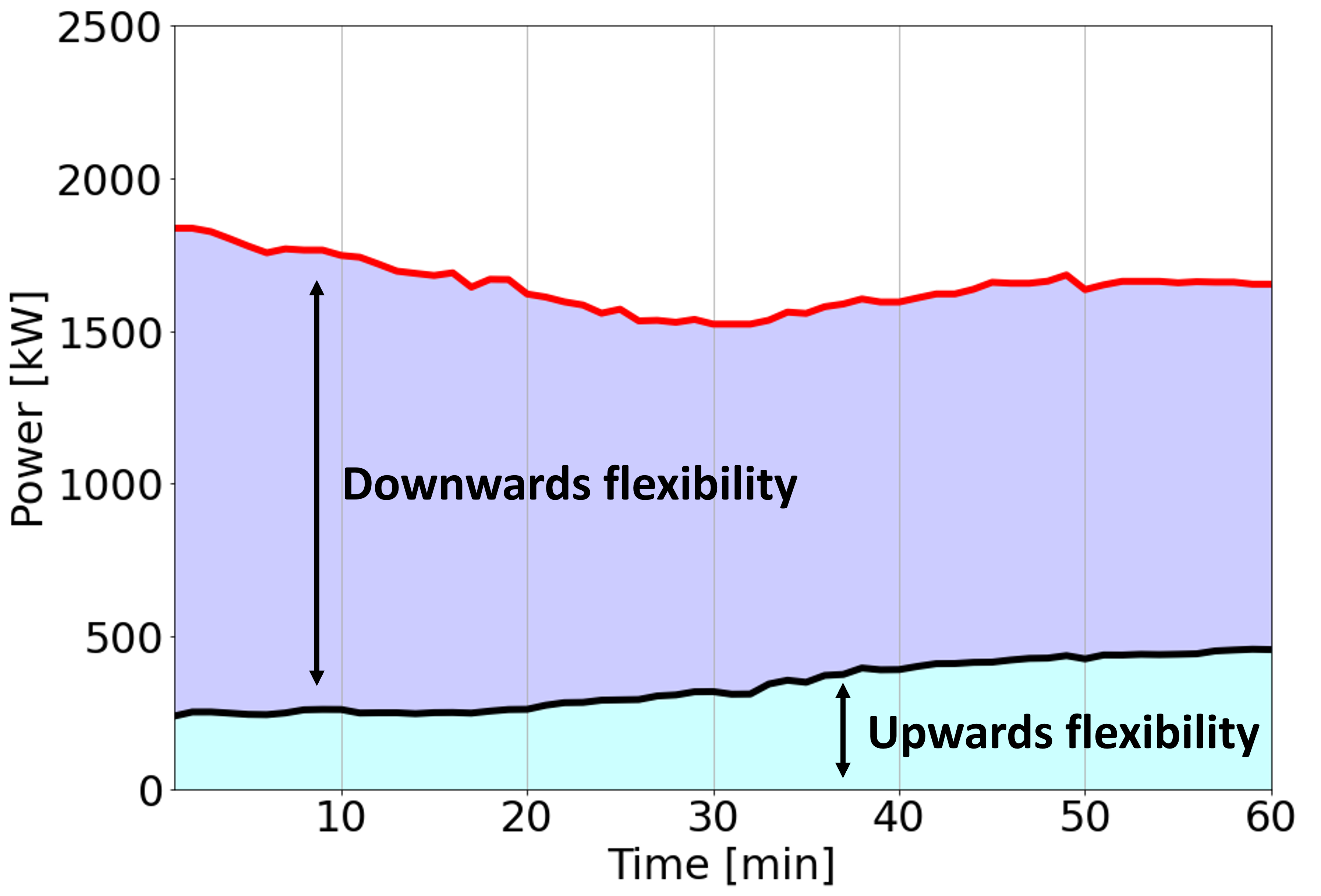
(b) 1,400 ev without LER req.

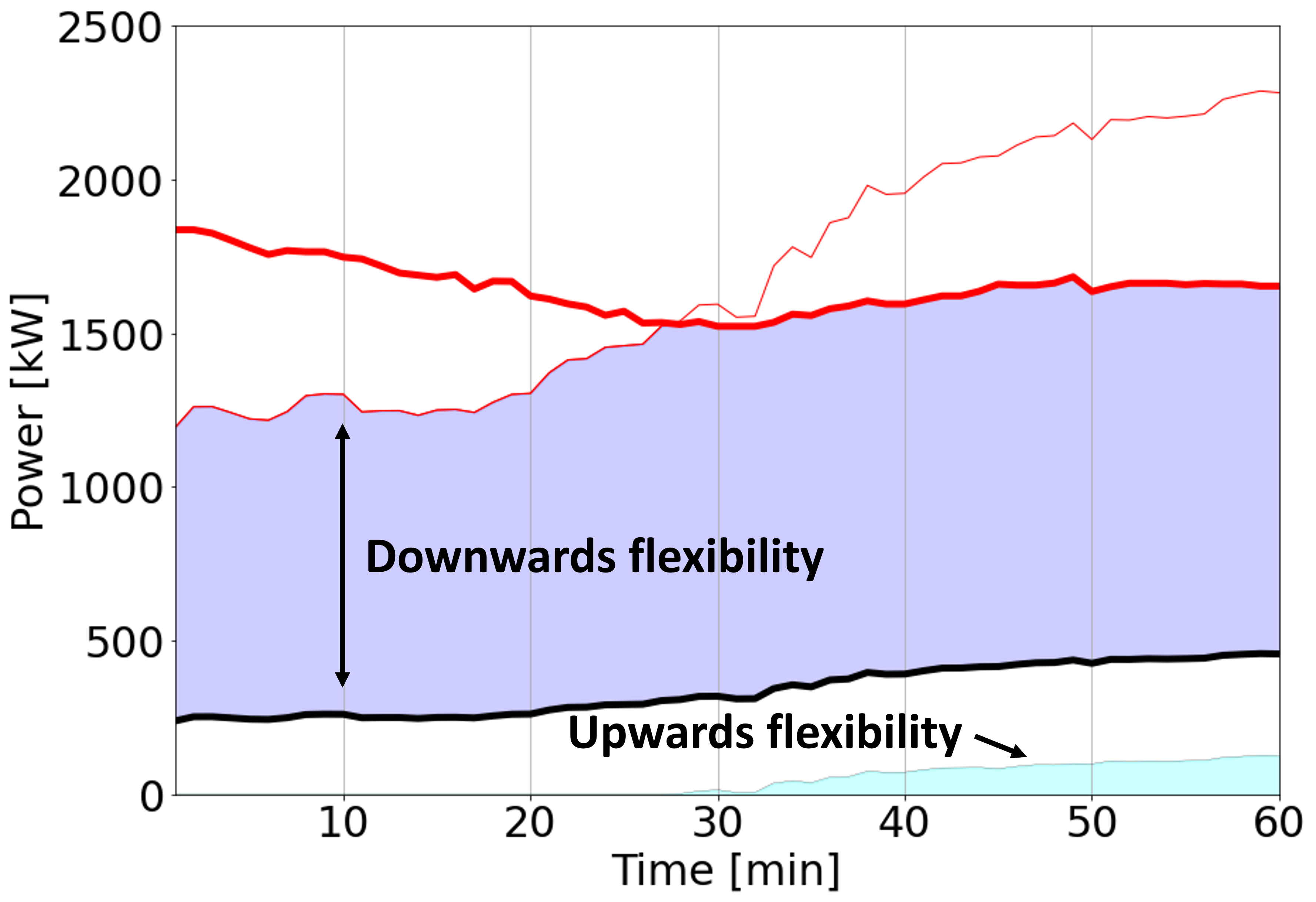
(c) 1,400 ev with 20% LER req.

Figure 3: The consumption of different portfolio sizes of ev either with or without the 20% LER requirements applied for a given sample hour.

Figure 4 shows how the flexibility is distributed throughout the day for a portfolio containing all 1400 ev. Each data point represents a given minute’s flexibility. The figure illustrates the bimodal nature of residential home charging with ev primarily charging in the evening and night.

The conditional cumulative distribution function describes the associated certainty of an aggregator having a flexibility higher than a given level. Generally, there is a larger spread in the distribution for the upwards flexibility, as shown in Figure 4(a), compared to the two other distributions, as illustrated in Figures 4(b) and 4(c). For example, at midday for upward regulation, there is a large right-tailed skewness in the data. Further, there is a large discrepancy between the available upward and downward flexibility, meaning the primary flexibility of ev consists of their ability to increase consumption. To compare the energy flexibility with the momentarily up and downwards, the energy can be converted into power by dividing it (kWh) by the duration of 20 minutes ($\frac{1}{3}$h). By doing so, two elements become apparent: (i) the energy flexibility will always be lower than the momentarily downward flexibility, hence making the constraint on $F^{\downarrow}$ redundant, and (ii), the energy flexibility is generally more than five times larger than the upward flexibility, meaning the binding ler requirement will presumably be the scarcity of upward flexibility. For notation ease, $F_{m}^{E}(\mathcal{\omega})$ is represented by its power property in the following mathematical models, while the constraint $F^{\downarrow}$ is for kept for consistency with Energinet’s documentation.

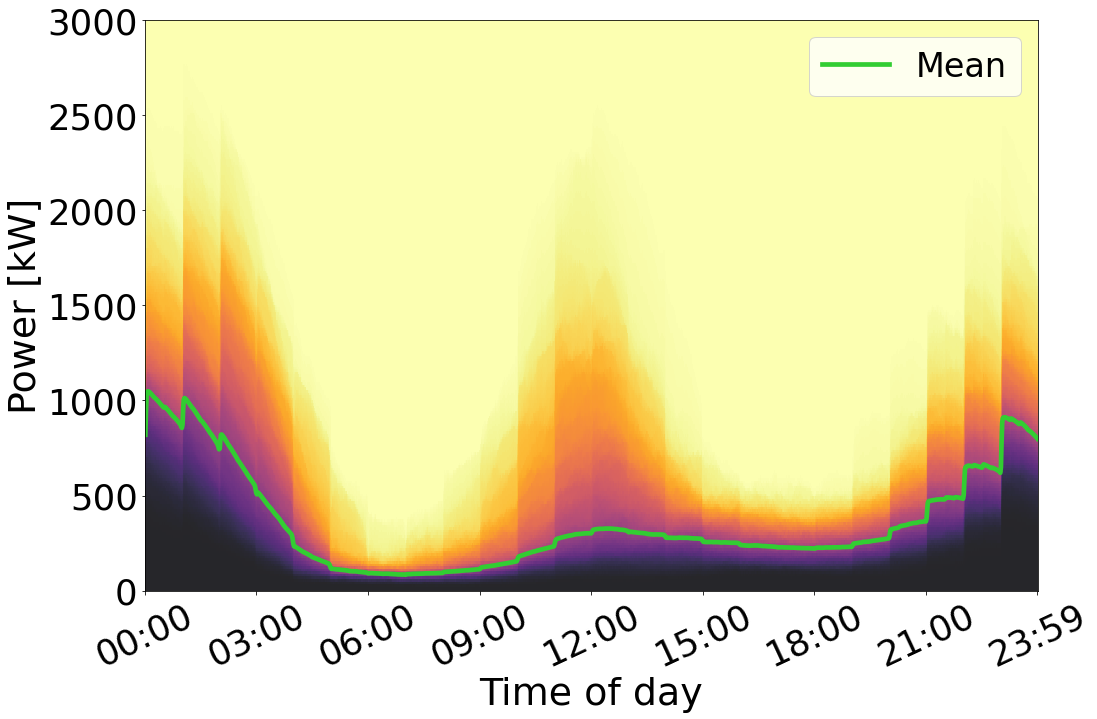
(a) Upwards flexibility $F^{\uparrow}$

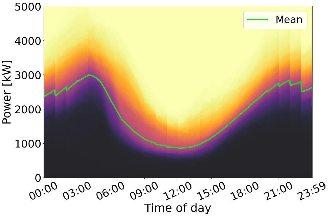
(b) Downwards flexibility $F^{\downarrow}$

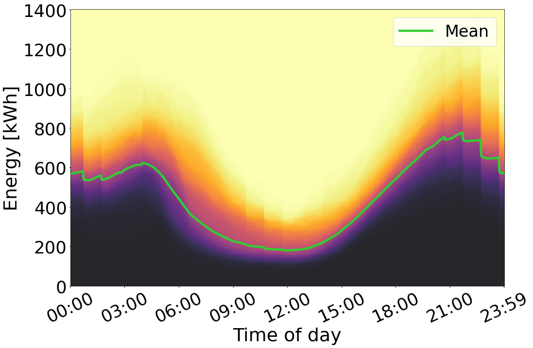
(c) Energy flexibility $F^{\mathrm{E}}$

Figure 4: Conditional cumulative distribution of available flexibility for a portfolio of 1,400 ev from March 24, 2022, to March 21, 2023.

III Simulation setup

This section describes the simulation setup used to investigate how an aggregator of ev can bid into fcrd in this paper. First, we revisit the time sequence for decision-making in our model, along with a cross-validation scheme to evaluate the model. Further, sampling of ev flexibility used for bidding is presented. Lastly, we define the synergy effect in terms of two metrics from which the aggregator’s bidding strategy is evaluated.

The code is publicly available at [31], although the ev data is proprietary.

III-A Evaluation strategy

We simulate the fcrd market in the three stages as previously illustrated in Figure 2. In the first stage, D$-1$, an aggregator makes upward and downward capacity bids $(c_{h}^{\mathrm{\uparrow}}$,$c_{h}^{\mathrm{\downarrow}})$, for each hour of the upcoming day, $D$. The bids are generated using samples $\omega\in\Omega$ of the uncertain available flexibility $F_{m,\omega}=(F^{\uparrow}_{m,\omega},F^{\downarrow}_{m,\omega},F^{\text{E}}_{m,\omega})$. A unique distribution of the available flexibility to each minute $m$ is thus made prior to the first stage from which $|\Omega|$ samples are drawn. The samples are drawn randomly without replacement for the first minute, while the samples for all other minutes depend on the day sampled in the previous minutes thus maintaining the correlation between minutes. The number of samples $|\Omega|$ is set to 216 according to [32] elaborated in Appendix A. Accordingly, all samples are assumed to be equiprobable.

As mentioned, stages two and three are merged into one stage. Here the set of uncertain parameters for day $D$ is realized, i.e., required activation power and realized available flexibility $F_{m}$. For all minutes, the bids are evaluated by assessing whether activation could be met, and if the full bid was possible to deliver. Thus, we define the maximum activation not met for both up and down-regulation for each hour as the penalty quantities $(p_{h}^{\uparrow},p_{h}^{\downarrow})$. Energinet defines the penalty cost as the substitution cost of replacing the missed activation. However, as no historical register of the replacement cost exists, the penalty costs $(\pi_{h}^{\uparrow},\pi_{h}^{\downarrow})$ are assumed to be five times the reservation prices $(\lambda_{h}^{\uparrow},\lambda_{h}^{\downarrow}$) which are historical volume-weighted average prices [28]. For simplicity, the profits/costs related to the energy delivery are considered negligible due to the low activation rate of fcrd. Accordingly, the objective of the aggregator is:

$$\underbrace{c^{\uparrow}\pi^{\uparrow}+c^{\downarrow}\pi^{\downarrow}}_{\text{Reservation payment}}-\underbrace{\lambda^{\uparrow}p^{\uparrow}-\lambda^{\downarrow}p^{\downarrow}}_{\text{Penalty cost}}$$ (1)

A three-fold cross-validation scheme is used to obtain oos results, where 363 days are randomly divided into three folds. The training fold consists of is flexibility, $F_{m,\omega}$, from which bids $(c^{\uparrow}_{h},c^{\downarrow}_{h})$ are derived using an optimization model (as explained in Section IV) while the test fold is used to evaluate the bids on realized portfolio flexibility, $F_{m}$, activation power, and fcrd prices. Hence, for each iteration in the cross-validation scheme, only one unique bid for up and down-regulation for each hour is made and evaluated on 121 days of the testing fold.

We note that this choice of cross-validation scheme is used to determine the historical performance of an aggregator bidding into fcrd for a portfolio of ev, which should be held up against a lookback strategy using, e.g., only most recent days in a rolling horizon manner. However, we emphasize that this paper is intended to provide an optimization model for how an aggregator can exploit the P90 rule for ler units, and not to provide the best possible model (which we leave for future work). To this end, a regular cross-validation scheme is suitable.

III-B Synergy effect

In this study, we hypothesize that the synergy effect of aggregating ev increases the quantities of flexibility bids for fcrd. To validate this hypothesis, two metrics are used. First, the aggregator profit as stated in (1), and second, the percentage of total flexibility bid, defined as

$$\text{Utilized bidding capacity}=\frac{c^{\downarrow}+c^{\uparrow}}{F^{\downarrow}+F^{\uparrow}}$$ (2)

An increase in both metrics thus indicates a synergy effect. Furthermore, a third metric is used to measure the compliance with the P90 rule, i.e., how often bids are higher than the realized flexibility (also called frequency of overbidding):

$$\text{Frequency of overbidding}=\frac{1}{H\times N}\sum_{m,h}y_{m,h}$$ (3)

Here, $y_{m,h}$ takes a value of one whenever an overbid occurs and zero if not, while $H$ denotes the number of hours and $N$ the number of minutes being tested for in the oos fold.

IV Mathematical modeling

In this section, we present the optimization problem that provides an optimal bidding strategy for an ev aggregator participating in fcrd adhering to the P90 rule using a jccp. First, a compact formulation of the problem is presented, followed by two reformulations: (i) ALSO-X [33] and (ii) CVaR [34]. The optimization problem is a one-stage stochastic program with uncertain power consumption of the ev portfolio, and therefore uncertain flexibility.

IV-A General mathematical formulation

As mentioned, only capacity bids are considered in this study since activation energy is negligible. We assume an ev portfolio can deliver the required frequency response as per the regulations [29]. The problem can thus simply be represented in a one-stage stochastic optimization model with a jcc representing the P90 rule with respect to available flexibility and ler requirements:

$$\underset{(c^{\downarrow},c^{\uparrow})\geq 0}{\text{Max}}\quad c^{\downarrow}+c^{\uparrow}$$ (4a)

s.t.

$$\mathbb{P}\left(\begin{array}[]{@{}l@{}}\frac{1}{5}c^{\downarrow}+c^{\uparrow}\leq F_{m}^{\uparrow}(\mathcal{\omega}),\quad\forall m\\ c^{\downarrow}\leq F_{m}^{\downarrow}(\mathcal{\omega}),\quad\forall m\\ c^{\downarrow}\leq F_{m}^{\mathrm{E}}(\mathcal{\omega}),\quad\forall m\end{array}\right)\geq 1-\epsilon$$ (4e)

Problem (4) looks to utilize as much of the ev’ flexible capacity as possible, and maximizes upward and downward flexibility. For simplicity, the Problem is decomposed per hour as there are no coupling constraints. The P90 rule applies across all ler requirements as seen in the jcc in (4e). It expresses that there should be at least $1-\epsilon$ probability that fcrd bids, $(c^{\mathrm{\uparrow}},c^{\mathrm{\downarrow}})$, adhere to all ler requirements as defined in Definition 1, for all minutes $m$ within a given hour. The first ler constraint states that the available upward flexibility, $F_{m}^{\uparrow}(\mathcal{\omega})$ in a given sample must be greater than the upward bid plus 20% of the downward bid for all minutes. Likewise, the second and third constraints state that the available downward flexibility, $F_{m}^{\downarrow}(\mathcal{\omega})$, and energy flexibility, $F_{m}^{E}(\mathcal{\omega})$, in a given sample, respectively, have to be greater than the downward bid for all minutes. The safety level $\epsilon$ is set to 0.1 as per Definition 2, hence allowing for a 10% risk of violating any of the three ler requirements. Thereby, (4e) fully adheres to the regulations for bidding uncertain demand into fcrd. To our knowledge, this is the first attempt at explicitly modeling the P90 rule and ler requirements using a jcc for fcrd.

IV-B Approximating jcc

jcc are generally computationally intractable [35]. In some cases, they can be reformulated analytically [36]. However, several approximations of jcc exist which provide a trade-off between optimality and computational speed. In this study, we opt for two different convex approximation approaches commonly used in the literature: (i) ALSO-X and (ii) cvar.

Both approximation methods are sample-based approaches, that reformulate Problem (4) to a lp using a finite set of samples $\omega\in\Omega$ drawn from historical data.

IV-B1 ALSO-X

The ALSO-X method [33] consists of two steps: a) Transforming the jccp to a milp and b) an iterative solution strategy. The corresponding milp for Problem (5) directly constrains the number of overbids by introducing binary variables $y_{m,\omega}$ and the Big-M method:

$$\underset{(c^{\downarrow},c^{\uparrow})\geq 0,y_{m,\omega}\in\{0,1\}}{\operatorname{Max}}c^{\downarrow}+c^{\uparrow}$$ (5a)

st.

$$\frac{1}{5}c^{\downarrow}+c^{\uparrow}-F^{\uparrow}_{m,\omega} \leq y_{m,\omega}M^{\uparrow} \forall m,\omega$$ (5b)

$$c^{\downarrow}-F^{\downarrow}_{m,\omega} \leq y_{m,\omega}M^{\downarrow} \forall m,\omega$$ (5c)

$$c^{\downarrow}-F^{\mathrm{E}}_{m,\omega} \leq y_{m,\omega}M^{E} \forall m,\omega$$ (5d)

$$\sum_{m}\sum_{\omega}y_{m,\omega} \leq q$$ (5e)

Constraints (5b)-(5d) represent the ler requirements, implying that $y_{m,\omega}=1$ if at least one of them is violated for a given minute. Constraint (5e) controls the frequency of overbid by counting the number of times that an overbid occurs using $y_{m,\omega}$. The count is then bound by the sum of $y_{m,\omega}$ for all minutes and samples. The upper bound is specified by parameter $q$, which is set according to the desired allowance rate, i.e., the P90 rule in Definition 2. Thus, $q$ represents the 10% overbid allowance, which equals $\lfloor\epsilon\cdot|\Omega|\cdot N\rfloor$, where $N$ is the number of minutes. The three Big M’s are set equal to the sample sets’ largest available flexibility.

Step b) in the ALSO-X algorithm obtains feasible solutions for Problem (5) that are computationally tractable as described in Algorithm 1.

Algorithm 1 ALSO-X

1:Input: Stopping tolerance parameter $\delta$

2:Require: $\text{Relax the integrality of }y$

3:$\underline{q}\leftarrow 0,\quad\bar{q}\leftarrow\lfloor\epsilon\times\Omega\times M\rfloor$

4:while $\bar{q}-\underline{q}\geq\delta$ do

5:     $\text{Set }q=\frac{(\underline{q}+\bar{q})}{2}$

6:     $\text{Retrieve }\Theta^{*}\text{ as an optimal solution to relaxed of}$

7:     Problem (5).

8:     $\text{Set }\underline{q}=q\text{ if }\mathbb{P}(y_{m,\omega}*=0)\geq 1-\epsilon\text{; otherwise, }\bar{q}=q$

9:end while

10:Output: A feasible solution to Problem (5)

The first step of the algorithm is to relax the integrality of $y$, i.e., $0\leq y\leq 1$. The relaxation converts the MILP to an LP thus providing convexity to the problem and making it faster to solve. To obtain a feasible solution to the original problem, $q$ is iteratively tightened as seen through steps 2 to 6 in Algorithm 1. The model terminates with a feasible solution once the lower and upper bound difference is less than $\delta$ which determines the threshold for convergence. In this study, setting $\delta$ to be $10^{-5}$ was found to provide an optimal trade-off between computational time and feasibility.

IV-B2 cvar

The cvar method [34] approximates the jcc by controlling magnitude of overbids using a reformulated lp. Thus, cvar minimizes the expected overbid violation for the worst $(1-\alpha)$ samples which is the var. Here $\alpha=0.1$ as per the P90 rule in Definition 2. The cvar approximation problem is shown in (6):

$$\underset{(c^{\downarrow},c^{\uparrow})\geq 0,\beta\leq 0,\zeta_{m,\omega}}{\operatorname{Maximize}}c^{\downarrow}+c^{\uparrow}$$ (6a)

st.

$$\frac{1}{5}c^{\downarrow}+c^{\uparrow}-F^{\uparrow}_{m,\omega} \leq\zeta_{m,\omega} \forall m,\omega$$ (6b)

$$c^{\downarrow}-F^{\downarrow}_{m,\omega} \leq\zeta_{m,\omega} \forall m,\omega$$ (6c)

$$c^{\downarrow}-F^{\mathrm{E}}_{m,\omega} \leq\zeta_{m,\omega} \forall m,\omega$$ (6d)

$$\sum_{m}\sum_{\omega}(\zeta_{m,\omega})\phi-(1-\alpha)\beta \leq 0$$ (6e)

$$\beta \leq\zeta_{m,\omega} \forall m,\omega$$ (6f)

The three ler constraints are shown in (6b)-(6d). $\zeta_{m,\omega}$ is an auxiliary variable that captures the potential overbid to each sample and links the risk across all three ler constraints. Further constraints (6e)-(6f) ensures that the model punishes making excessive overbids and conservative bids, by respectively stating that the average $\zeta_{m,\omega}$ has to be below var, and the implantation of $\beta$ as well as forcing it to take the lowest $\zeta_{m,\omega}$.

In summary, the cvar approximation in (6) looks to optimize the aggregator’s bids based on the worst samples determined by the var risk level. Given the structure of the problem, it often leads the method to find the optimal cvar threshold to be around the average missing subset below var, ultimately leading cvar to be a conservative approximation method [37].

V Results and discussion

In this section, we show the synergy effect of aggregating ev for bidding into fcrd while adhering to the P90 rule and the ler requirements using the reformulations presented in the previous section and simulation setup described in Section III. Furthermore, an Oracle model with perfect foresight of the available ev flexibility will serve as an upper bound for the monetary potential.

We start by assessing the synergy effect by presenting by solving (4) for different portfolio sizes. Here, the metrics for synergy defined in (1), (2), and (3) are used. Second, the sensitivity of the ler regulation is evaluated. Lastly, we investigate how the optimization model exploits the P90 rule with respect to the frequency of overbids.

V-A Synergy effect

Figure 5 shows the average hourly profit for all three models subject to eight different portfolio configurations with bundle sizes of 70, 28, 14, 10, 7, 4, 2, and 1, meaning that for a specific configuration, the 1,400 ev will be divided into one of the bundles. When assessing a specific portfolio configuration, the total bid capacity and profit are determined by adding the capacities and profits across all bundles. Thus, the comparison of ALSO-X and cvar results are ensured to be comparable.

Overall, Figure 5 reveals a significant synergy effect, as increasing the portfolio sizes within each bundle consistently increases earnings. The synergy effect occurs immediately, whereafter the gradient decreases during the last steps, indicating a diminishing return rate (although more ev would be needed to conclude this). Increasing the portfolio size thus leverages the P90 rule as uncertainty in realized ev consumption, and thereby flexibility, is reduced. This interim finding is supported by comparing it to the Oracle model, where the relative difference in earnings decreases for larger portfolio sizes. However, even when bundling all 1,400 ev into a single portfolio, the Oracle method outperforms the stochastic methods by a factor of two to three. This indicates that a significant unfilled potential lies in improving the representation of the probabilistic expectation of flexibility for the ev used in this study.

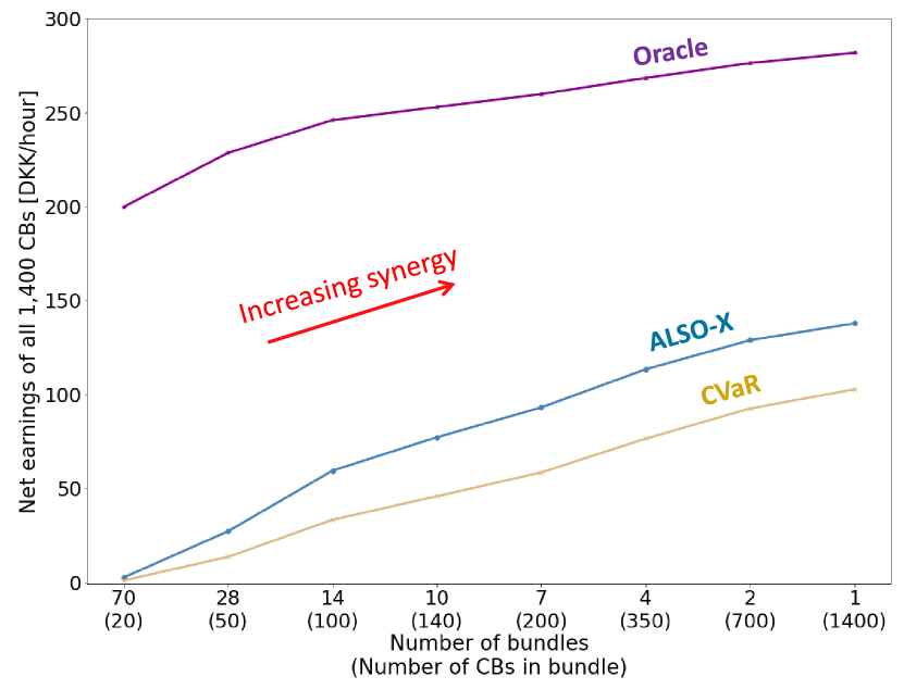
Figure 5: Mean hourly earnings for all 1,400 ev for different bundle configurations. The hourly mean is determined oos for all 363 days using three-fold cross-validation as described in Section III.

Table I underpins these findings as it shows how the Oracle model bids a significantly higher proportion of the available flexibility. Looking at the approximations, ALSO-X manages to bid more flexibility than cvar and thus outperforms cvar from a monetary point of view. The same is seen in Figure 5, where ALSO-X’s higher bids explicitly correspond to higher profits.

An average ev included in the portfolio of 1,400 ev would earn an annual profit of $857$ DKK using ALSO-X and $638$ DKK with cvar, respectively bidding 24.4% and 18.5% of the total flexibility. Hence, from an aggregator’s perspective, there is a significant monetary benefit of pooling all available ev and by using ALSO-X as opposed to cvar. However, cvar might prove better for new, unseen data in non-stationary environments. For example, as new ev join the portfolio or when grid tariffs change due to political decisions. In these cases, ALSO-X is fairly aggressive and is not guaranteed to adhere to the P90 rule while cvar is much more conservative.

	CVaR	ALSO-X	Oracle
Upwards flexibility	2.0%	4.7%	40.0%
Downwards flexibility	10.8%	16.0%	40.0%
Overall	9.5%	14.0%	40.0%

TABLE I: Average percentage of utilized bidding capacity bid across the 1,400 ev for all bundle sizes.

V-B Relaxation of ler regulation

Interestingly, all three models are far from bidding 100% of their total flexibility. In particular, it is noteworthy that the Oracle model only bid $40$% of its total available flexibility. This is due to two factors: (i) Bids are required to be uniform within hours, meaning some flexibility is simply lost and (ii) as illustrated in Figure 3, subsets of both upward and downward flexibility are inaccessible due to the ler requirements of reserving 20% of the downward bid in upward flexibility. Little upward flexibility is directly bid into the market, as it is reserved to facilitate the downward bid. The downwards bids are restrained by the discrepancy between downward and upward flexibility often being greater than a factor of five, as illustrated in Figures 4(a) and 4(b), which ultimately causes a lot of downwards capacities to be unavailable.

The impact of relaxing the ler constraints, is presented in Table II. Here, the portfolio of 1,400 ev is tested on two relaxed sets of ler requirements using the ALSO-X bidding scheme. In the testing case referred to as energy relaxation, the rule of reserving 20% of the downwards capacity bid in upwards flexibility is removed, while the 20 duration requirements are removed in the testing case referred to as energy relaxation. In the upwards relaxation case upwards flexibility is not required reserved for downwards bids, meaning a massive increase in upwards flexibility bid, while it also enables extra downwards capacity bid. For the energy relaxation case, the downward bids also increase, concluding the energy reservoir indeed is limiting the bids in the base case. However, the upward flexibility bid decreases, as a larger quantity of it is reserved to facilitate the extra enabled downward capacity. The general results signify the immense influence of the specific constraint. In particular, the upwards relaxation is binding, as the total amount of flexibility bid increases from 24.4% to 35.6%, with an annual revenue increase of $61$%. Consequently, the ler requirements are particularly constraining for an ev aggregator and perhaps of concern to the tso as less flexibility is being procured.

Figure 6 illustrates the case where the average downward bids are placed relative to the distribution of available flexibility for the three cases. It reveals that bids in the relaxed cases are generally placed closer to the 10% risk level allowed by the P90 rule. Further, it illustrates how each of the two LER requirements is the binding constraint for the base ler case at different timesteps. The base ler’s downward bids are bounded by its energy reservoir level between 22:00-03:00 and 10:00-14:00, as the energy relaxation produces larger bids, while the base case follows the bids in the upwards relaxation case in these hours. As illustrated in Figures 4(a) and 4(b) these are hours where the average discrepancy between upwards and downwards flexibility is lower than a factor of five, meaning there is enough upwards flexibility to facilitate the full downwards flexibility being bid. In the remaining hours, the discrepancy is larger than a factor of five, thus indicating that it is a shortage of upward flexibility that restrains the downward capacity bid. Accordingly, both requirements established to handle duration issues are restraining the bids, with the constraint on the upward flexibility especially being the most restraining.

From an aggregator’s perspective, the challenges of the ler regulations could be mitigated by increasing the heterogeneity of its portfolio. Here, it would be beneficial to include technologies with more upward flexibility, and a more diverse consumption pattern, allowing for a more consistent soc of its energy reservoir during the day. From a system perspective, the tso might be interested in carefully assessing the ler requirements as Figure 6 and Table II clearly shows how liquidity increases when relaxing them. Ultimately, it is a trade-off between the security of supply, liquidity, and costs, as more liquidity drives down tso expenditure per MW of fcrd, but decreases the security of supply. Further research is needed to determine the exact added security of supply of the ler requirements. However, they are in place to ensure the duration of the bid capacity, which might be insignificant to the security of supply, as longer activation periods hardly ever occur. Therefore, it would be of interest to analyze alternative approaches for preserving the security of supply.

	Annual profit	$\uparrow$ utilized bidding capacity	$\downarrow$ utilized bidding capacity
Base LER	1,200 kDKK	8.6%	27.3%
Upwards relaxation	1,934 kDKK	36.4%	35.4%
Energy relaxation	1,344 kDKK	3.1%	32.8%

TABLE II: Synergy metrics evaluated oos for a 1,400 ev portfolio using the ALSO-X approximation over all 363 days with three-folded cross-validation as described in Section III.

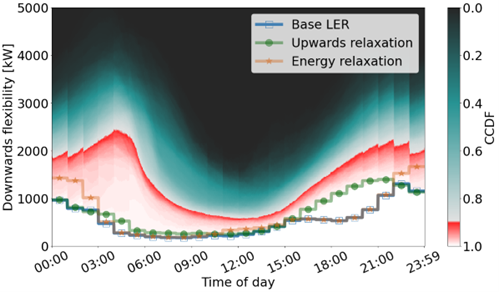
Figure 6: The average amount of downwards flexibility bid using ALSO-X and a portfolio size of 1,400 ev with and without the respective ler requirements of 20 minutes of continuous down-regulation (Energy) and 20% capacity reservation in the opposite direction (Upwards).

V-C Frequency of overbid

We now compare ALSO-X and cvar with respect to the compliance of the P90 rule. Figure 7 shows cvar and ALSO-X daily frequency of overbidding for the portfolio of 1,400 ev. ALSO-X hits the desired allowance rate of $10$% almost perfectly, as the frequency of overbid across all simulated days is $10.15$%. cvar is well below the threshold as only $3.89$% of all minutes are overbids. cvar has 190 days with no overbids altogether, and almost no days exceeding the exclusion rate of $15$%. The spread amongst the days is broader for ALSO-X, with a larger subset of days above the exclusion threshold. The individual days with very large overbids are not a problem according to Definition 2 of the P90 rule, as it refers to the average violation rate over the whole inspection period, which is required to be a minimum of three months. Hence, both bidding schemes adhere to the P90 rule.

Nonetheless, if the sample period was shorter, ALSO-X could potentially violate the P90 rule as there exist subsets that go above the $15$% excluding threshold, whereas cvar supplies more security in that regard. Hence, the methods present a trade-off between potential profits and security of supply, meaning even though ALSO-X seems preferable from a profit viewpoint, cvar could be preferable, as it is inherently conservative and offers a margin for error with respect to the P90 rule. From a system perspective, the tso gets less liquidity in the market if aggregators and other service providers use robust approaches like cvar, but more security of supply, and vice versa if methods like ALSO-X is used which fully exploit the rule set.

Having an adequate representation of the uncertain available flexibility $F=(F^{\uparrow}$, $F^{\downarrow}$, $F^{E})$ is thus especially important if applying ALSO-X, while cvar would be more likely to produce feasible results oos with an inaccurate representation.

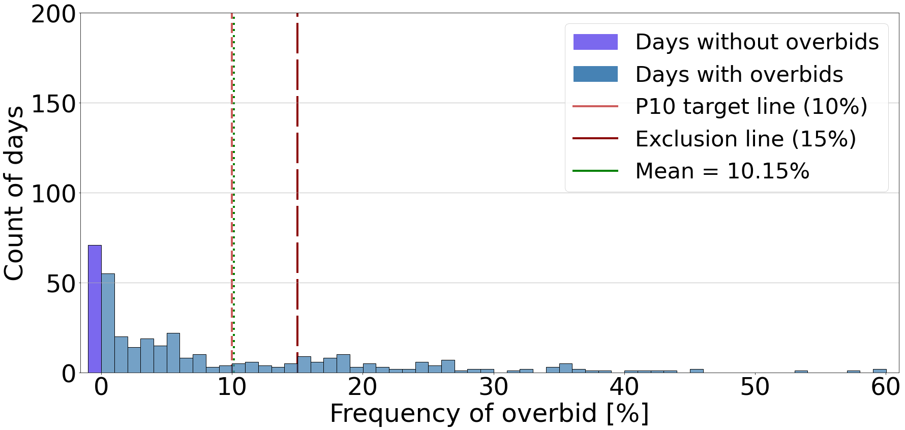
(a) ALSO-X

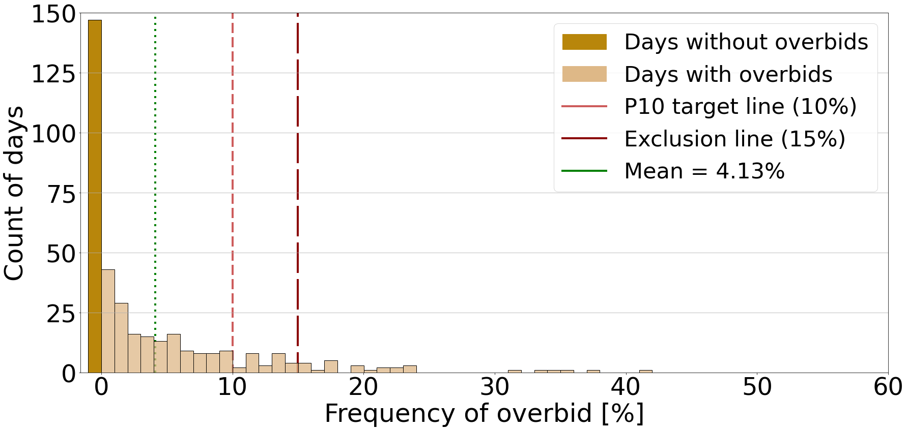
(b) cvar

Figure 7: Frequency of overbids tested for a portfolio of 500 ev for cvar and ALSO-X for 363 days.

VI Conclusion and future work

The stability of the future power grid is challenged by increased renewable and less stable fossil-fuel-based generation. Demand flexibility contains significant, untapped potential in this regard. We investigated how a portfolio of grid-connected ev can deliver fcrd in Denmark through an aggregator, thus earning money while balancing large frequency disturbances in the power grid. We showed how an aggregator can model the newly invented P90 from the Danish tso while adhering to ler requirements using a jccp with two approximations: (i) ALSO-X and (ii) cvar.

A significant synergy was identified upon aggregation of ev, as the quantity of flexibility enabled for fcrd bidding increased for larger portfolios, yielding higher aggregator profits and less uncertainty of available flexibility. cvar appeared as a conservative approximation method compared to ALSO-X. ALSO-X fully explored the allowed frequency of overbids, i.e., the 10% threshold, while cvar’s rate of overbids was less than half of ALSO-X’s, thus not leveraging the full potential of the P90 rule.

In general, bids were especially limited by the ler constraint reserving 20% of the downward bid in upward flexibility. Hence, future work should investigate how these challenges could be mitigated, as it would be of interest for both the aggregator and the tso to leverage more of the portfolio flexibility into the market. From the aggregator perspective, we suggest introducing a more diverse technology portfolio, which could further reduce the uncertainty of available flexibility. From a tso’s perspective, it would be of interest to further compare the added security of supply versus exposed liquidity and procurement costs when modifying the ler constraints. Here the requirement of reserving 20% flexibility in the opposite direction to control the SoC was found significantly more constraining than the 20-minute full response requirement.

Other avenues of future research should explore the influence of the simplifications and assumptions inherent in this study. Moreover, our rather simplistic approach to the probabilistic representation of the underlying flexibility of the ev portfolio is an element with potential for improvement, highlighted by the large discrepancy between the stochastic and Oracle models. We recommend aggregators develop a more advanced forecasting method such as generalized linear models. Furthermore, distributionally robust optimization can help in cases where the empirical distribution of the underlying flexibility is misspecified.

Appendix A: Number of samples

Various approaches exist for selecting the number of samples for stochastic optimization as seen in [36, 24, 25] where an empirical approach is used and numerical results are tested subject to different sample sizes, while [38, 39] uses analytical approaches. In this study, we have opted to use a theoretical number of samples as seen in (7) [33]:

$$N\geq\frac{2}{\epsilon}\log\left(\frac{1}{\delta}\right)+2n+\frac{2n}{\epsilon}\log\left(\frac{2}{\epsilon}\right)\rightarrow N\geq 216$$ (7)

Here, multiple parameters are selected according to the given problem. First, $\epsilon\in(0,1)$ is the argument denoting the acceptable failure rate of the jcc, which is set to 0.1 based on Energinet’s P90 requirement. Second, $n$ denotes the dimensionality of the model, which translates to the number of decision variables (i.e., two). Third, $\delta\in(0,1)$ denotes the confidence level of the probabilistic constraint holding. Accordingly, $\delta$ is selected such that there is $1-\delta$ probability that the model’s decisions ($c^{\uparrow},c^{\downarrow}$) are a feasible solution in the $\epsilon$-level problem formulation. We set $\delta$ to $0.01$, allowing a 1% risk a given hour to violate the P90 rule. The relative high-risk rate is chosen, as the P90 allows for 5% room for error, while the evaluation is on the average violation frequency, allowing more risk on individual bids.

We note the (7) only holds when the underlying data-generating process is stationary which might not be the case in reality. However, it works well within a cross-validation framework to showcase the synergy effect of aggregating ev, and to demonstrate the efficacy of the jccp representing the P90 rule.

References

- [1] F. The Nordic TSOs (Svenska kraftnät, Energinet and Statnett), “Nordic grid development perspective 2023,” 2023. [Online]. Available: https://www.statnett.no/globalassets/for-aktorer-i-kraftsystemet/planer-og-analyser/ngpd2023.pdf
- [2] Energinet, “Outlook for ancillary services 2023-2040,” Online, 2023, accessed: 04-03-2024. [Online]. Available: https://energinet.dk/media/gieparrh/outlook-for-ancillary-services-2023-2040.pdf
- [3] N. E. M. Group, “Distributed flexibility – lessons learned in the nordics,” 2022. [Online]. Available: https://www.nordicenergy.org/publications/distributed-flexibility-lessons-learned-in-the-nordics/
- [4] I. R. E. Agency. (2019) Demand-side flexibility for power sector transformation. Online.
- [5] C. Ziras, C. Heinrich, and H. W. Bindner, “Why baselines are not suited for local flexibility markets?” Renewable and Sustainable Energy Reviews, vol. 135, p. 110357, 2021.
- [6] P. A. Gade, T. Skjøtskift, H. W. Bindner, and J. Kazempour, “Ecosystem for demand-side flexibility revisited: The Danish solution,” The Electricity Journal, vol. 35, no. 9, p. 107206, 2022.
- [7] Energinet (Danish TSO), “Prequalification of units and aggregated portfolios,” 2023. [Online]. Available: https://en.energinet.dk/Electricity/Ancillary-Services/Prequalification-and-test
- [8] B. Biegel, M. Westenholz, L. H. Hansen, J. Stoustrup, P. Andersen, and S. Harbo, “Integration of flexible consumers in the ancillary service markets,” Energy, vol. 67, pp. 479–489, 2014.
- [9] Energinet, “Scenarierapport 2022-2032,” Online, 2022, accessed: 05-03-2024. [Online]. Available: https://energinet.dk/media/k4kb5i3x/scenarierapport-2022-2032.pdf
- [10] D. E. M. Bondy, G. T. Costanzo, K. Heussen, and H. W. Bindner, “Performance assessment of aggregation control services for demand response,” pp. 1–6, 2014.
- [11] B. Biegel, L. H. Hansen, J. Stoustrup, P. Andersen, and S. Harbo, “Value of flexible consumption in the electricity markets,” Energy, vol. 66, pp. 354–362, 2014.
- [12] I. M. Casla, A. Khodadadi, and L. Söder, “Optimal day ahead planning and bidding strategy of battery storage unit participating in nordic frequency markets,” IEEE Access, vol. 10, pp. 76 870–76 883, 2022.
- [13] M. Seo, Y. Jin, M. Kim, H. Son, and S. Han, “Strategies for electric vehicle bidding in the german frequency containment and restoration reserves market,” Electric Power Systems Research, vol. 228, p. 110040, 2024.
- [14] P. Ponnaganti, R. Sinha, J. R. Pillai, and B. Bak-Jensen, “Flexibility provisions through local energy communities: A review,” Next Energy, vol. 1, no. 2, p. 100022, 2023.
- [15] M. Gržanić, T. Capuder, N. Zhang, and W. Huang, “Prosumers as active market participants: A systematic review of evolution of opportunities, models and challenges,” Renewable and Sustainable Energy Reviews, vol. 154, p. 111859, 2022.
- [16] A. Dogan, “Analyzing flexibility options for microgrid management from economical operational and environmental perspectives,” International Journal of Electrical Power and Energy Systems, vol. 158, p. 109914, 2024.
- [17] T. Baroche, F. Moret, and P. Pinson, “Prosumer markets: A unified formulation,” pp. 1–6, 2019.
- [18] S. de la Torre, J. Aguado, and E. Sauma, “Optimal scheduling of ancillary services provided by an electric vehicle aggregator,” Energy, vol. 265, p. 126147, 2023.
- [19] P. Astero and C. Evens, “Optimum day-ahead bidding profiles of electrical vehicle charging stations in fcr markets,” Electric Power Systems Research, vol. 190, p. 106667, 2021.
- [20] A. Thingvad, C. Ziras, G. L. Ray, J. Engelhardt, R. R. Mosbæk, and M. Marinelli, “Economic value of multi-market bidding in nordic frequency markets,” in 2022 International Conference on Renewable Energies and Smart Technologies (REST), vol. I, 2022, pp. 1–5.
- [21] “Aggregated demand-side energy flexibility: A comprehensive review on characterization, forecasting and market prospects,” Energy Reports, vol. 8, pp. 9344–9362, 2022.
- [22] P. A. V. Gade, T. Skjøtskift, H. W. Bindner, and J. Kazempour, “Synergy among flexible demands: Forming a coalition to earn more from reserve market,” in Proceedings of IEEE International Conference on Communications, Control, and Computing Technologies for Smart Grids (IEEE SmartGridComm). United States: IEEE, 2023.
- [23] A. Porras Cabrera, C. Dominguez, J. Morales, and S. Pineda, “Tight and compact sample average approximation for joint chance constrained optimal power flow,” 05 2022.
- [24] A. Esteban-Pérez and J. M. Morales, “Distributionally robust optimal power flow with contextual information,” European Journal of Operational Research, vol. 306, no. 3, pp. 1047–1058, 2023.
- [25] C. Ordoudis, V. A. Nguyen, D. Kuhn, and P. Pinson, “Energy and reserve dispatch with distributionally robust joint chance constraints,” Operations Research Letters, vol. 49, no. 3, pp. 291–299, 2021.
- [26] N. Jiang and W. Xie, “Also-x and also-x+: Better convex approximations for chance constrained programs,” Operations Research, vol. 70, no. 6, pp. 3581–3600, 2022.
- [27] M. Kuivaniemi, “Frequency - historical data,” Accessed Month 2023, fingrid Oyj dataset on the frequency of the Nordic synchronous system. [Online]. Available: https://data.fingrid.fi/en/dataset/frequency-historical-data
- [28] Energi Data Service, “Fcr-n d-2,” https://www.energidataservice.dk/tso-electricity/FcrNdDK2, accessed: 2024-02-28.
- [29] Energinet (Danish TSO), “Prequalification of units and aggregated portfolios,” 2023, version 2.0. [Online]. Available: https://energinet.dk/media/r0rbaoqb/prequalification-of-units-and-aggregated-portfolios.pdf
- [30] B. M. Car and Driver, “Electric car battery life: Everything you need to know,” Online, 2022, accessed: 02-03-2024. [Online]. Available: https://www.caranddriver.com/research/a31875141/electric-car-battery-life/
- [31] (2024) Github codebase. [Online]. Available: https://github.com/lunde77/Thesis
- [32] J. Luedtke and S. Ahmed, “A sample approximation approach for optimization with probabilistic constraints,” SIAM Journal on Optimization, vol. 19, no. 2, pp. 674–699, 2008.
- [33] S. Ahmed, J. Luedtke, Y. Song, and W. Xie, “Nonanticipative duality, relaxations, and formulations for chance-constrained stochastic programs,” Mathematical Programming, 2017.
- [34] R. T. Rockafellar, S. Uryasev et al., “Optimization of conditional value-at-risk,” Journal of risk, vol. 2, pp. 21–42, 2000.
- [35] R. DING, G.-X. LI, and Q.-Q. LI, “Robust approximations to joint chance-constrained problems,” Acta Automatica Sinica, vol. 41, no. 10, pp. 1772–1777, 2015.
- [36] K. Baker and A. Bernstein, “Joint chance constraints in ac optimal power flow: Improving bounds through learning,” IEEE Transactions on Smart Grid, vol. 10, no. 6, pp. 6376–6385, 2019.
- [37] S. Sarykalin, G. Serraino, and S. Uryasev, Value-at-Risk vs. Conditional Value-at-Risk in Risk Management and Optimization, ch. Chapter 13, pp. 270–294.
- [38] K. Margellos, P. Goulart, and J. Lygeros, “On the road between robust optimization and the scenario approach for chance constrained optimization problems,” IEEE Transactions on Automatic Control, vol. 59, no. 8, pp. 2258–2263, 2014.
- [39] L. A. Roald, “Optimization methods to manage uncertainty and risk in power systems operation,” 2016.