Generative Modelling with High-Order Langevin Dynamics

Abstract

Diffusion generative modelling (DGM) based on stochastic differential equations (SDEs) with score matching has achieved unprecedented results in data generation. In this paper, we propose a novel fast high-quality generative modelling method based on high-order Langevin dynamics (HOLD) with score matching. This motive is proved by third-order Langevin dynamics. By augmenting the previous SDEs, e.g. variance exploding or variance preserving SDEs for single-data variable processes, HOLD can simultaneously model position, velocity, and acceleration, thereby improving the quality and speed of the data generation at the same time. HOLD is composed of one Ornstein-Uhlenbeck process and two Hamiltonians, which reduce the mixing time by two orders of magnitude. Empirical experiments for unconditional image generation on the public data set CIFAR-10 and CelebA-HQ show that the effect is significant in both Frechet inception distance (FID) and negative log-likelihood, and achieves the state-of-the-art FID of 1.85 on CIFAR-10.

1 Introduction

Diffusion generative model (DGM) is characterized by gradually adding noise to the target data until it becomes the data conforming to some simple prior distribution. The earliest such model is proposed by [Sohl-Dickstein et al.(2015)Sohl-Dickstein, Weiss, Maheswaranathan, and Ganguli] in the field of image generation, and then generalized by [Ho et al.(2020)Ho, Jain, and Abbeel] and [Song et al.(2020b)Song, Sohl-Dickstein, Kingma, Kumar, Ermon, and Poole], which proposed DGM based on denoising score matching with Langevin dynamics to achieve the quality that surpasses generative adversarial network (GAN) [Goodfellow et al.(2014)Goodfellow, Pouget-Abadie, Mirza, Xu, Warde-Farley, Ozair, Courville, and Bengio] or variational autoencoder (VAE) [Kingma and Welling(2014)]-based generation methods in the field of high-resolution high-quality image generation. Then, in just two years, DGM made unprecedented progress and has achieved success in many fields such as image editing [Meng et al.(2021)Meng, Song, Song, Wu, Zhu, and Ermon], natural language processing [Li et al.(2022)Li, Thickstun, Gulrajani, Liang, and Hashimoto], text-to-image [Rombach et al.(2022)Rombach, Blattmann, Lorenz, Esser, and Ommer], and so on.

In addition to applying DGM to different fields, another aspect of research is how to improve the existing DGM itself, so that the quality of the generated data is higher and the speed of generation is faster. There are two types of DGM, one is discrete [Ho et al.(2020)Ho, Jain, and Abbeel, Bao et al.(2022)Bao, Li, Sun, Zhu, and Zhang] and the other is continuous [Song et al.(2020b)Song, Sohl-Dickstein, Kingma, Kumar, Ermon, and Poole, Dockhorn et al.(2021)Dockhorn, Vahdat, and Kreis]. For an efficient discrete DGM, we need to design an ingenious noise scheduling with a finite length Markov chain to gradually realize the mutual conversion between data and white noise. While for continuous DGM, the main task is to design a good stochastic differential equation (SDE) and a corresponding integrator. This paper mainly explores new possibilities in continuous DGM.

Recently there has been a lot of research work on continuous DGM, such as designing different integrators, or fast solvers for revserse-time SDEs with trained scoring models [Dockhorn et al.(2022)Dockhorn, Vahdat, and Kreis, Liu et al.(2022)Liu, Ren, Lin, and Zhao, Bao et al.(2022)Bao, Li, Sun, Zhu, and Zhang, Lu et al.(2022)Lu, Zhou, Bao, Chen, Li, and Zhu]. This paper focuses on another direction, which is to improve the SDE itself in the forward diffusion process [Dockhorn et al.(2021)Dockhorn, Vahdat, and Kreis, Wang et al.(2021)Wang, Jiao, Xu, Wang, and Yang]. Inspired by critically-damped Langevin diffusion (CLD) [Dockhorn et al.(2021)Dockhorn, Vahdat, and Kreis] and the work of [Mou et al.(2021)Mou, Ma, Wainwright, Bartlett, and Jordan], we propose high-order Langevin dynamics (HOLD) to further decouple the position variables from the Brownian motion by introducing new intermediate variables. Most of the SDEs used for generate modelling are first-order for data variables (such as images or 3D models, etc.), but theoretically, we can formally introduce any number of intermediate variables into these SDEs, such as

$$\begin{cases}&d{\mathbf{x}}_{1}={\mathbf{x}}_{2}dt,\\ &d{\mathbf{x}}_{2}=-L^{-1}\nabla V({\mathbf{x}}_{1})dt+\gamma{\mathbf{x}}_{3}dt,\\ &\quad\cdots\\ &d{\mathbf{x}}_{n-1}=-L^{-1}\nabla V({\mathbf{x}}_{n-2})dt+\gamma{\mathbf{x}}_{n}dt,\\ &d{\mathbf{x}}_{n}=-\gamma{\mathbf{x}}_{n-1}dt-\xi{\mathbf{x}}_{n}dt+\sqrt{2\xi L^{-1}}d{\mathbf{w}}_{t},\end{cases}$$ (1)

so that the Brownian motion $\sqrt{2\xi L^{-1}}d{\mathbf{w}}_{t}$ can only affect the position (data) variable ${\mathbf{x}}_{1}$ after $n-1$ times of conduction through the intermediate variables ${\mathbf{x}}_{2},\cdots,{\mathbf{x}}_{n}$, then the final path of the position variable will be much smoother. Eq. (1) is called high-order Langevin dynamics (HOLD), which will be used as the forward diffusion dynamics for our newly proposed DGM. In HOLD, two adjacent variables can form a Hamiltonian dynamics

$$\vspace{0.2cm}\begin{cases}&d{\mathbf{x}}_{i-1}=\gamma{\mathbf{x}}_{i}dt,\\ &d{\mathbf{x}}_{i}=-L^{-1}\nabla V({\mathbf{x}}_{i-1})dt\end{cases}\vspace{-0.2cm}$$ (2)

and the Brownian motion only directly affects the last variable ${\mathbf{x}}_{n}$. That is to say, HOLD consists of $n-1$ Hamiltonian components and one Ornstein-Uhlenbeck (OU) process. And each of these Hamiltonian dynamics can quickly traverse the data space and reduce the mixing time of the system [Neal(2011)]. To verify our idea, we use a third-order Langevin dynamics [Mou et al.(2021)Mou, Ma, Wainwright, Bartlett, and Jordan] (refer to Eq. (6) and for convenience it is also referred to as HOLD hereinafter ) to implement the forward diffusion process. This HOLD can simulate position, velocity, and acceleration simultaneously, where the position variable does not directly depend on the energy gradient and Brownian component, which are separated by velocity and acceleration. Only the acceleration depends explicitly on the random component. Figure 1 gives a one-dimensional example, and it can be seen that the solution path of DGM based on HOLD is gentler and smoother than that of CLD and variance preservering (VP) SDE. This results in fewer steps to generate high-quality data, which means faster generation.

Our HOLD has been extensively testified on sevaral public benchmarks. It is shown that HOLD-based DGM admits easy-to-tune hyperparameters, better synthesis quality, shorter mixing times, and faster sampling. Our tailor-made solver for HOLD-DGM far surpasses other methods. On the CIFAR-10 and CelebA real-world image modelling task, HOLD-based DGM outperforms various state-of-the-art methods in synthesis quality under similar computation resources. Last but not least, we find an excellent computationally efficient instance for HOLD-DGM in the vast ocean of third-order stochastic Langevin dynamics.

2 Background

Itô linear SDE is an excellent and tractable model for converting between data of different probability distributions [Song et al.(2020b)Song, Sohl-Dickstein, Kingma, Kumar, Ermon, and Poole]. The general form of Itô linear SDE is as follows

$$d{\mathbf{q}}_{t} ={\bm{f}}(t){\mathbf{q}}_{t}\,dt+{\bm{G}}(t)\,d{\mathbf{w}}_{t},\quad t\in[0,T],$$ (3)

where ${\mathbf{q}}_{t}\in\mathbb{R}^{d}$ is the position vector of a particle (represents the data that needs to be generated in DGM, such as images or 3D models, etc.), ${\bm{f}}(t),{\bm{G}}(t)\in\mathbb{R}^{d\times d}$, ${\bm{f}}(t){\mathbf{q}}_{t}$ is the drift coefficient, ${\bm{G}}(t)$ is the diffusion coefficient, and ${\mathbf{w}}_{t}$ is the standard Wiener process. First-order continuous-time Langevin dynamics are a special case of stochastic process represented by the SDE (3) [Mou et al.(2021)Mou, Ma, Wainwright, Bartlett, and Jordan]. Let $p({\mathbf{q}}_{t},t)$ be the probability density of the stochastic process ${\mathbf{q}}_{t}$ at time $t$. This SDE (3) transforms the beginning data distribution $p({\mathbf{q}}_{0},0)$ into a final simple tractable latent distribution $p({\mathbf{q}}_{T},T)$ by gradually adding the noise from ${\mathbf{w}}_{t}$.

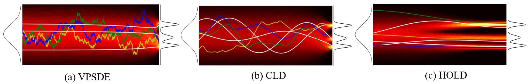
Figure 1: Comparison of solution paths between HOLD-based DGM and other methods on 1D data. The paths in white are obtained by integrating the corresponding ODE flows. The coloured paths are obtained by solving the corresponding backward generative SDE with Euler-Maruyama method.

If the solution process ${\mathbf{q}}_{t}$ can be reversed in time, the target image or 3D data can be generated from a simple latent distribution. Indeed the time-reverse process is the solution of the corresponding backward SDE [Anderson(1982)]

$$d{\mathbf{q}}_{t}=\left[{\bm{f}}(t){\mathbf{q}}_{t}-{\bm{G}}(t){\bm{G}}(t)^{\top}\nabla_{{\mathbf{q}}_{t}}\log p({\mathbf{q}}_{t},t)\right]dt+{\bm{G}}(t)d\overline{{\mathbf{w}}}_{t}$$ (4)

for $0\leq t\leq T$, where $\overline{{\mathbf{w}}}_{t}$ is the standard Wiener process in reverse time. Therefore, it can be seen that the key to generative modelling with SDE lies in the calculations of $\nabla_{{\mathbf{q}}_{t}}\log p({\mathbf{q}}_{t},t)$, $(0\leq t\leq T)$, which is always called score function [Hyvärinen and Dayan(2005), Song et al.(2020b)Song, Sohl-Dickstein, Kingma, Kumar, Ermon, and Poole]. And the score function can be obtained by optimizing the denoising score matching (DSM) loss [Hyvärinen and Dayan(2005), Vincent(2011)]

$$\text{DSM loss}=\mathbb{E}_{t\sim[0,T]}\mathbb{E}_{{\mathbf{q}}_{0}\sim p_{data}({\mathbf{q}}_{0},0)}\mathbb{E}_{{\mathbf{q}}_{t}\sim p({\mathbf{q}}_{t}|{\mathbf{q}}_{0})}\left[\frac{1}{2}\parallel\mathfrak{S}_{\theta}({\mathbf{q}}_{t},t)-\nabla_{{\mathbf{q}}_{t}}\log p({\mathbf{q}}_{t}|{\mathbf{q}}_{0})\parallel^{2}\right].$$ (5)

After the score function $\mathfrak{S}_{\theta}({\mathbf{q}}_{t},t)$ is learned, then the Langevin Markov chain Monte Carlo (MCMC) or the discretized time-reverse SDE (4) can be used to generate large-scale data in target distribution.

3 Generative Modelling with High-Order Langevin Dynamics

First-order continuous-time Langevin dynamics and score matching are key to the success of SDE-based DGM [Song et al.(2020b)Song, Sohl-Dickstein, Kingma, Kumar, Ermon, and Poole] and its following work [Song et al.(2021)Song, Durkan, Murray, and Ermon]. Although the continuous-time Langevin dynamics converges to the target distribution at an exponential rate, the error caused by discretization in practice makes the mixing time only $O(d/\epsilon^{2})$ [Mou et al.(2021)Mou, Ma, Wainwright, Bartlett, and Jordan], where $\epsilon>0$ is the Wasserstein distance from the target distribution. We propose to use high-order lifting to generalize and move this idea to higher-order continuous dynamics, such that momentum (also referred to as velocity) and acceleration are introduced to accelerate the convergence and enhance the sampling quality of position vectors.

3.1 Third-Order Langevin Dynamics

We model the forward diffusion process as the solution of the following third-order Itô SDE

$$\begin{cases}d{\mathbf{q}}_{t}&={\mathbf{p}}_{t}dt,\\ d{\mathbf{p}}_{t}&=-L^{-1}\nabla U({\mathbf{q}}_{t})dt+\gamma{\mathbf{s}}_{t}dt,\\ d{\mathbf{s}}_{t}&=-\gamma{\mathbf{p}}_{t}dt-\xi{\mathbf{s}}_{t}dt+\sqrt{2\xi L^{-1}}d{\mathbf{w}}_{t}\end{cases}$$ (6)

where ${\mathbf{q}}_{t},{\mathbf{p}}_{t},{\mathbf{s}}_{t}\in\mathbb{R}^{d}$ are the position, momentum (first row in Eq. (6) implies that ${\mathbf{p}}_{t}$ is the time derivative of position ${\mathbf{q}}_{t}$), and acceleration processes respectively, $L$ is the Lipschitz constant of $U$, $\gamma>0$ is the friction coefficient, and $\xi>0$ is an algorithmic parameter. In the modelling equation of momentum, $U({\mathbf{q}}_{t}):\mathbb{R}^{d}\to\mathbb{R}$ is the potential function related to the position vector. In this paper, we employ $U({\mathbf{q}}_{t})=\frac{L}{2}\norm{{\mathbf{q}}_{t}}$ which is strongly convex and Lipschitz smooth. Let ${\mathbf{x}}_{t}=({\mathbf{q}}_{t},{\mathbf{p}}_{t},{\mathbf{s}}_{t})^{\top}\in\mathbb{R}^{3d}$, the SDE (6) can be written in matrix form $d{\mathbf{x}}_{t}={\bm{f}}(t){\mathbf{x}}_{t}\,dt+{\bm{G}}(t)\,d{\mathbf{w}}_{t}$, where ${\bm{f}}(t)$ and ${\bm{G}}(t)$ are

$$\begin{pmatrix}0&1&0\\ -1&0&\gamma\\ 0&-\gamma&-\xi\end{pmatrix}\otimes{\bm{I}}_{d},\begin{pmatrix}0&0&0\\ 0&0&0\\ 0&0&\sqrt{2\xi L^{-1}}\end{pmatrix}\otimes{\bm{I}}_{d},$$ (7)

respectively, here $\otimes$ denotes the Kronecker product. Considering the computability, especially the complexity and the expressiveness, after trial and error, we let $\gamma^{2}=1+\frac{\xi^{2}}{4}$ in this paper. Since then ${\bm{f}}(t)$ has three different real eigenvalues in elegant and simple closed form, which are $-\frac{\xi}{2}$ and $-\frac{\xi\pm\sqrt{\xi^{2}-32}}{4}$. This will make the mean and variance of the transition densities

$$p({\mathbf{x}}_{t}|{\mathbf{x}}_{0},t)={\mathcal{N}}({\mathbf{x}}_{t};{\bm{\mu}}_{t},{\bm{\Sigma}}_{t}),\quad{\bm{\Sigma}}_{t}=\Sigma_{t}\otimes{\bm{I}}_{d},$$ (8)

$$\Sigma_{t}=\begin{pmatrix}\Sigma_{t}^{qq}&\Sigma_{t}^{qp}&\Sigma_{t}^{qs}\\ \Sigma_{t}^{qp}&\Sigma_{t}^{pp}&\Sigma_{t}^{ps}\\ \Sigma_{t}^{qs}&\Sigma_{t}^{ps}&\Sigma_{t}^{ss}\end{pmatrix}$$ (9)

of the solution process ${\mathbf{x}}_{t}$ feasible to calculate. It can be shown that the prior distribution (or equilibrium distribution) of this diffusion is $p_{\infty}({\mathbf{x}})=\mathcal{N}({\mathbf{q}};\bm{0}_{d},\frac{\xi L^{-1}}{6}{\bm{I}}_{d})\,\mathcal{N}({\mathbf{p}};\bm{0}_{d},\frac{\xi L^{-1}}{6}{\bm{I}}_{d})\,\mathcal{N}({\mathbf{s}};\bm{0}_{d},\frac{\xi L^{-1}}{6}{\bm{I}}_{d})$. As introduced in Section 1, the dynamics of Eq. (6) is referred to as HOLD hereinafter.

There are two Hamiltonian components $({\mathbf{p}}_{t}dt,-{\mathbf{q}}_{t}dt)^{\top}$ and $(\gamma{\mathbf{s}}_{t}dt,-\gamma{\mathbf{p}}_{t}dt)^{\top}$, and one Ornstein-Uhlenbeck (OU) process $(-\xi{\mathbf{s}}_{t}dt+\sqrt{2\xi L^{-1}}d{\mathbf{w}}_{t})$ in HOLD (6) with coefficients (7). Hamiltonian components can make two successive sampling points in the Markov chain far apart, so that a representative sampling of a canonical distribution can be obtained with fewer iterations. Hamiltonian dynamics allows the Markov chain to explore target distribution much more efficiently [Neal(2011)]. Two Hamiltonian can lead to twice the convergence speedup. The OU process has a bounded variance and admits a stationary probability distribution. It has a tendency to move back towards a central location, with a greater attraction when the process is further away from the center [Särkkä and Solin(2019)]. That is to say, all three components that make up HOLD contribute to the fast traversal of the solution space.

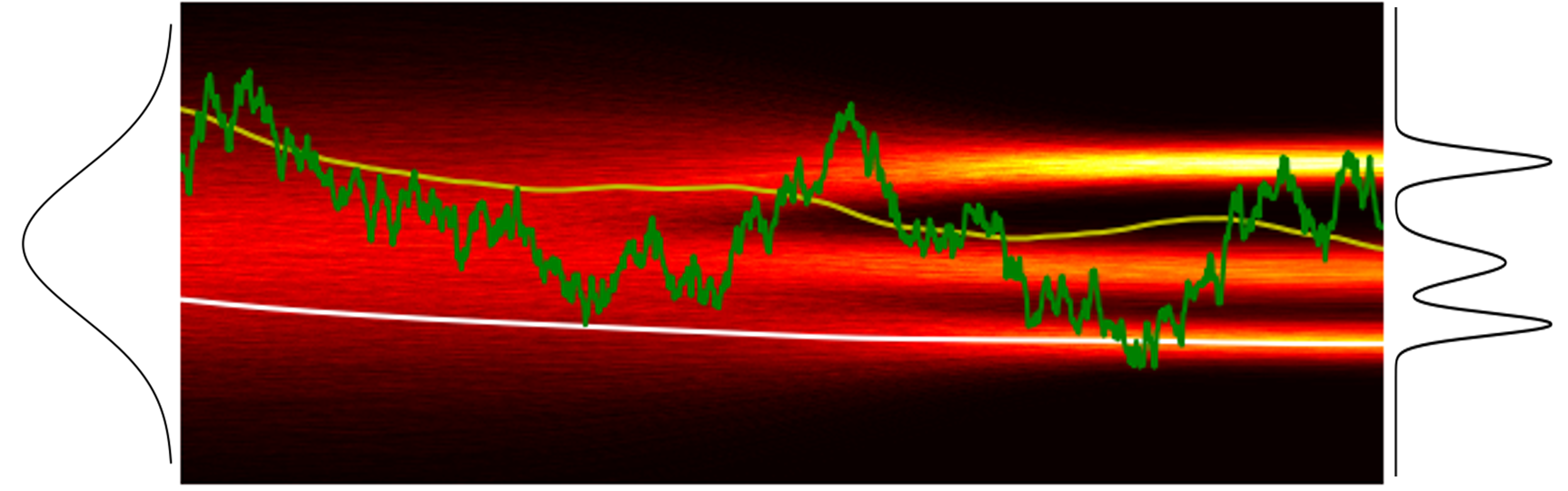
Figure 2: In 1D case, the solution (data generation) paths of the position (white), velocity (yellow), and acceleration (green) variables in HOLD.

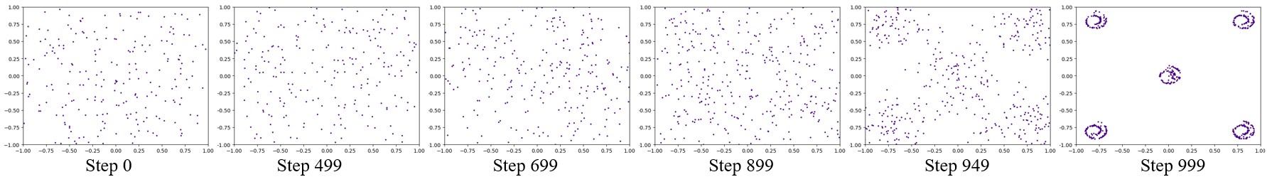
(a) 2D multi-Swiss rolls generated by CLD-based DGM at 6 moments along the solution path.

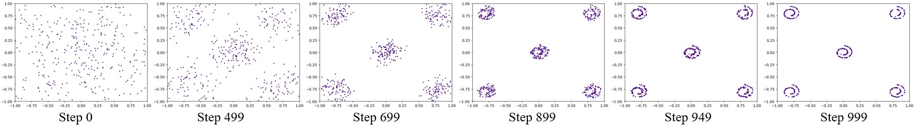
(b) 2D multi-Swiss rolls generated by HOLD-based DGM at 6 moments along the solution path.

Figure 3: Comparison of different moments (number of steps) on the solution path generated by CLD and HOLD-based DGM on 2D multi-Swiss rolls.

Looking at Eq. (6) from an intuitive point of view, random noise can directly affect ${\mathbf{s}}_{t}$, while ${\mathbf{s}}_{t}$ can only affect ${\mathbf{q}}_{t}$ indirectly through ${\mathbf{p}}_{t}$, so it can be expected that ${\mathbf{q}}_{t}$ is relatively smooth. The trajectory ${\mathbf{q}}_{t}$ under these third-order dynamics have two additional orders of smoothness compared to the Wiener process ${\mathbf{w}}_{t}$. They are smoother than the corresponding trajectories under underdamped or critically damped Langevin dynamics [Mou et al.(2021)Mou, Ma, Wainwright, Bartlett, and Jordan, Dockhorn et al.(2021)Dockhorn, Vahdat, and Kreis]. This higher smoothness degree can better control the discretization error. Figure 2 shows a one-dimensional example of HOLD. It can be seen that ${\mathbf{q}}$ can converge faster than ${\mathbf{p}}$ and ${\mathbf{s}}$. It has been proved by [Mou et al.(2021)Mou, Ma, Wainwright, Bartlett, and Jordan] that certain discretization schemes of Eq. (6) can generate data from the canonical distribution in $O(d^{1/4}/\epsilon^{1/2})$ steps, which is (smoother and) exponentially faster than all the sampling scheme based on Eq. (3), e.g. variance exploding (VE) or variance preserving (VP) SDEs [Song et al.(2020b)Song, Sohl-Dickstein, Kingma, Kumar, Ermon, and Poole]. Figures 3 and 4 show the generation of a complex multiple 2-dimensional Swiss rolls. Under the same conditions, it can be seen that HOLD has a better synthesis effect and a more stable generation speed than CLD. For example, Figure 3 shows that at step 699, it has been able to see that the sampling points have been gathered around the five cluster centers in HOLD, while the sampling points in CLD still look completely noisy.

3.2 Block Coordinate Score Matching

The key to using SDE for generation is the estimation of the score function, and the current best estimation method is based on DSM loss (5). In the derivation of DSM loss for HOLD-based DGM, most of the elements in the matrix $G(t)G(t)^{\top}\otimes{\bm{I}}_{d}$ are 0, except for the sub-matrix $2\xi L^{-1}\otimes{\bm{I}}_{d}$ in the lower right corner. So in $\nabla_{{\mathbf{x}}_{t}}$ only the derivatives with respect to the entries in ${\mathbf{s}}_{t}$ are not zero.

Since the numerical value of the score function $\nabla_{{\mathbf{s}}_{t}}\log p({\mathbf{x}}_{t}\mid{\mathbf{x}}_{0},t)$ in the DSM loss is not within a bounded domain, and its estimation is often unstable, especially as the time $t$ tends to zero. By Eq. (8) we have $\nabla_{{\mathbf{x}}_{t}}\log p({\mathbf{x}}_{t}\mid{\mathbf{x}}_{0},t)=-{\bm{L}}_{t}^{-\top}{\mathbf{\epsilon}}_{3d}$, where ${\mathbf{\epsilon}}_{3d}\sim{\mathcal{N}}(\bm{0},{\bm{I}}_{3d})$ and ${\bm{\Sigma}}_{t}={\bm{L}}_{t}{\bm{L}}_{t}^{\top}$ is the Cholesky factorization of the covariance matrix ${\bm{\Sigma}}_{t}$. The noise ${\mathbf{\epsilon}}_{3d}$ is confined to a small bounded cubic almost all the time. Therefore it is better to predict the noise than the score itself, which has also been proved in the experiments by [Kim et al.(2021)Kim, Shin, Song, Kang, and Moon] and [Song and Ermon(2020)]. Methods based on noise prediction always lead to better Frechet inception distance (FID) [Ho et al.(2020)Ho, Jain, and Abbeel, Rombach et al.(2022)Rombach, Blattmann, Lorenz, Esser, and Ommer]. In experiments and applications, it is assumed ${\bm{\mu}}_{0}=({\mathbf{q}}_{0},\bm{0}_{d},\bm{0}_{d})$, and $\Sigma_{0}^{qq}=0,\Sigma_{0}^{pp}=\alpha L^{-1},\Sigma_{0}^{ss}=\alpha L^{-1}$ ( ${\bm{\Sigma}}_{0}=\mathrm{diag}(\Sigma_{0}^{qq},\Sigma_{0}^{pp},\Sigma_{0}^{ss})\otimes{\bm{I}}_{d}$ ), where $\alpha\ll 1$. Then $p({\mathbf{x}}_{t}\mid{\mathbf{x}}_{0},t)=p({\mathbf{x}}_{t}\mid{\mathbf{q}}_{0},t)$. By reparameterization of $\nabla_{{\mathbf{s}}_{t}}\log p_{t}({\mathbf{x}}_{t}\mid\cdot)=-\ell_{t}{\mathbf{\epsilon}}_{2d:3d}$, the DSM loss (5) is reformulated as

$$\mathbb{E}_{{\mathbf{x}}_{0}\sim p({\mathbf{x}}_{0}),{\mathbf{\epsilon}}_{3d}\sim{\mathcal{N}}(\bm{0},{\bm{I}}_{3d})}\left[\ell_{t}^{2}\norm{{\mathbf{\epsilon}}_{2d:3d}+\mathfrak{E}_{\theta}({\bm{\mu}}_{t}+{\bm{L}}_{t}{\mathbf{\epsilon}}_{3d},t)}_{2}^{2}\right].$$

where $\mathfrak{E}_{\theta}({\bm{\mu}}_{t}+{\bm{L}}_{t}{\mathbf{\epsilon}}_{3d},t)=\mathfrak{S}_{\theta}({\bm{\mu}}_{t}+{\bm{L}}_{t}{\mathbf{\epsilon}}_{3d},t)/\ell_{t}$, and $1/\ell_{t}$ is

$$\sqrt{\Sigma^{ss}_{t}-\frac{(\Sigma^{sq}_{t})^{2}}{\Sigma^{qq}_{t}}-\left(\Sigma^{pp}_{t}-\frac{\left(\Sigma^{pq}_{t}\right)^{2}}{\Sigma^{qq}_{t}}\right)^{-1}\left(\Sigma^{sp}_{t}-\frac{\Sigma^{sq}_{t}\Sigma^{pq}_{t}}{\Sigma^{qq}_{t}}\right)^{2}}.$$

It is obvious that ${\bm{\mu}}_{t}$, ${\bm{L}}_{t}$, and $\Sigma_{t}$s all have ${\mathbf{x}}_{0}$ in their argument.

For general high-order dynamics, there are multiple variables (several blocks of coordinates), e.g. for third-order Langevin dynamic system in Eq. (6), only one block ${\mathbf{q}}$ to represent the variables of interest and other two blocks ${\mathbf{p}}$ and ${\mathbf{s}}$ are introduced just to allow the two Hamiltonian dynamics to operate. There is no obvious reason that we need to denoise all blocks [Dockhorn et al.(2021)Dockhorn, Vahdat, and Kreis]. Thus in this paper we propose block coordinate score matching (BCSM) to denoise only initial distribution ${\mathbf{b}}_{0}$ for part of all blocks ${\mathbf{x}}_{0}$, and marginalize over the distribution $p({\mathbf{x}}_{0}\backslash{\mathbf{b}}_{0})$ of remaining variables, which result in

$${\mathcal{L}}_{\mathrm{BCSM}}\coloneqq\mathbb{E}_{t\sim{\mathcal{U}}[0,T]}\lambda(t)\mathbb{E}_{{\mathbf{b}}_{0}\sim p({\mathbf{b}}_{0}),{\mathbf{x}}_{t}\sim p({\mathbf{x}}_{t}\mid{\mathbf{b}}_{0},t)}\left[\norm{\nabla_{{\mathbf{s}}_{t}}\log p({\mathbf{x}}_{t}\mid{\mathbf{b}}_{0},t)-\mathfrak{S}_{\theta}({\mathbf{x}}_{t},t)}_{2}^{2}\right].$$ (10)

BCSM is a flexible objective, and the only requirement for ${\mathbf{b}}_{0}$ is that it must contain block ${\mathbf{q}}_{0}$, which is the variable we are interested in. BCSM is also equivalent to SM, which is proved in the App. 9.4. After re-parameterization, the BCSM is

$$\mathbb{E}_{t\sim{\mathcal{U}}[0,T]}\lambda(t)\mathbb{E}_{{\mathbf{b}}_{0}\sim p({\mathbf{b}}_{0}),{\mathbf{x}}_{t}\sim p({\mathbf{x}}_{t}\mid{\mathbf{b}}_{0},t)}\left[\norm{-\ell^{BCSM}_{t}{\mathbf{\epsilon}}_{2d:3d}-\mathfrak{S}_{\bm{\theta}}({\mathbf{x}}_{t},t)}_{2}^{2}\right],$$ (11)

which is the format used in our implementation. The intuition behind BCSM is that the distribution of $q_{0}$ is complex and unknown, and the distribution of $s_{0}$ is known, easy and fixed. That is to say, BCSM is easier to optimize, and ablation experiments also show that BCSM is better than the original DSM.

4 Lie-Trotter Sampler (for HOLD-DGM)

Methods of sampling from a continuous diffusion generation model defined by an SDE are generally divided into two categories, one is based on the corresponding time-reverse SDE, e.g. Euler-Maruyama (EM) [Song et al.(2020b)Song, Sohl-Dickstein, Kingma, Kumar, Ermon, and Poole], GGF [Jolicoeur-Martineau et al.(2021)Jolicoeur-Martineau, Li, Piché-Taillefer, Kachman, and Mitliagkas], the other is based on the ODE flow corresponding to the reverse SDE, e.g. RK45 [Dormand and Prince(1980)], DEIS [Zhang and Chen(2022)], DPM-Solver [Lu et al.(2022)Lu, Zhou, Bao, Chen, Li, and Zhu], GENIE [Dockhorn et al.(2022)Dockhorn, Vahdat, and Kreis], etc. Among them, there are many acceleration algorithms based on ODE flow, because there is no random item, the direction of the path can be more accurately predicted.

This paper proposes a new sampling method inspired by molecular dynamics and thermodynamics [Tuckerman(2010), Leimkuhler and Matthews(2015)]. The sampling problem is solved by the Lie-Trotter method, also known as the split operator method [Trotter(1959)]. The principle of the Lie-Trotter method is to decompose a complex operator into two or more operators that are easy to calculate and iterate repeatedly. Below we introduce how this principle is applied to the sampling of DGM based on HOLD.

After we obtain the optimal predictor $\mathfrak{S}_{\bm{\theta}}({\mathbf{x}}_{t},t)$ for score $\nabla_{{\mathbf{s}}_{t}}\log p({\mathbf{x}}_{t},t)$, which can be plugged into the backward HOLD for denoising the prior distribution into the target data. The backward or the generative HOLD is approximated with

$$d{\mathbf{q}}_{t} =-{\mathbf{p}}_{t}dt,$$

$$d{\mathbf{p}}_{t} ={\mathbf{q}}_{t}dt-\gamma{\mathbf{s}}_{t}dt,$$ (12)

$$d{\mathbf{s}}_{t} =\gamma{\mathbf{p}}_{t}dt+\xi{\mathbf{s}}_{t}dt+2\xi L^{-1}\mathfrak{S}_{\bm{\theta}}({\mathbf{x}}_{t},t)dt+\sqrt{2\xi L^{-1}}d\bar{\mathbf{w}}_{t}.$$

We regard the right side of the backward HOLD (12) as the superposition of multiple different vector fields, and the principle of decomposition is that the SDE or differential equation (DE) corresponding to individual vector field has an exact solution. The exact solution here means that it is possible to sample from the distribution corresponding to this component. Assume $p({\mathbf{x}}_{0},0)$ is an initial distribution in the phase space, then the propagation is determined $p({\mathbf{x}}_{t},t)=e^{t\mathcal{L}_{H}^{\dagger}}p({\mathbf{x}}_{0},0)$ where $\mathcal{L}_{H}^{\dagger}$ is the Fokker-Planck operator for time reverse HOLD (12) and $p({\mathbf{x}}_{t},t)$ is the evolved distribution at time $t$. From experience in solving higher-order SDE equations (1), in particular the previous estimates of transition probability kernels for third-order Langevin dynamical systems (6), we have exact closed-form solutions for the superimposition of Ornstein-Uhlenbeck process and the sum of the two Hamiltonian components. So we first isolate the following SDE from the right side of the backward Eq. (12)

$$\begin{pmatrix}d{\mathbf{q}}_{t}\\ d{\mathbf{p}}_{t}\\ d{\mathbf{s}}_{t}\end{pmatrix}=\begin{pmatrix}-{\mathbf{p}}_{t}\\ {\mathbf{q}}_{t}-\gamma{\mathbf{s}}_{t}\\ \gamma{\mathbf{p}}_{t}-\xi{\mathbf{s}}_{t}\end{pmatrix}dt+\begin{pmatrix}\bm{0}_{d}\\ \bm{0}_{d}\\ \sqrt{2\xi L^{-1}}d\bar{\mathbf{w}}_{t}\end{pmatrix}.$$ (13)

It is different from Eq. (6), but very similar, so many calculations related to Eq. (6) can be extended to Eq. (13). And the remaining vector field is

$$\begin{pmatrix}d{\mathbf{q}}_{t}\\ d{\mathbf{p}}_{t}\\ d{\mathbf{s}}_{t}\end{pmatrix}=\begin{pmatrix}\bm{0}_{d}\\ \bm{0}_{d}\\ 2\xi\left[L^{-1}\mathfrak{S}_{\bm{\theta}}({\mathbf{x}}_{t},t)+{\mathbf{s}}_{t}\right]\end{pmatrix}dt.$$ (14)

Let $\mathcal{L}_{A}^{\dagger}$ and $\mathcal{L}_{B}^{\dagger}$ be the Fokker-Planck operators of SDE (13) and DE (14) respectively. Thus we have $\mathcal{L}_{H}^{\dagger}=\mathcal{L}_{A}^{\dagger}+\mathcal{L}_{B}^{\dagger}$ and $e^{t\mathcal{L}_{H}^{\dagger}}=e^{t\left(\mathcal{L}_{A}^{\dagger}+\mathcal{L}_{B}^{\dagger}\right)}$. It is easy to verify that $\mathcal{L}_{A}^{\dagger}$ and $\mathcal{L}_{B}^{\dagger}$ cannot be exchanged (commute). Fix a constant valued function $p$ and we can see that $\mathcal{L}_{A}^{\dagger}\mathcal{L}_{B}^{\dagger}(p)\neq 0$, while $\mathcal{L}_{B}^{\dagger}\mathcal{L}_{A}^{\dagger}(p)=0$. Thus the classical propagator $e^{t\left(\mathcal{L}_{A}^{\dagger}+\mathcal{L}_{B}^{\dagger}\right)}$ cannot be separated into a simple product $e^{t\mathcal{L}_{A}^{\dagger}}e^{t\mathcal{L}_{B}^{\dagger}}$. This is unfortunate because in many cases the effect of the individual operators $e^{t\mathcal{L}_{A}^{\dagger}}$ and $e^{t\mathcal{L}_{B}^{\dagger}}$ on the phase space vector can be precisely evaluated. So it would be useful if the commutator could be represented by these two factors. In fact, there is a way to do this using an important theorem called Trotter’s theorem [Trotter(1959)]. The theorem states that for two operators $\mathcal{L}_{A}^{\dagger}$ and $\mathcal{L}_{B}^{\dagger}$

$$e^{t\mathcal{L}_{A}^{\dagger}+t\mathcal{L}_{B}^{\dagger}}=\lim_{P\to\infty}\left[e^{\frac{t\mathcal{L}_{A}^{\dagger}}{2P}}e^{\frac{t\mathcal{L}_{B}^{\dagger}}{P}}e^{\frac{t\mathcal{L}_{A}^{\dagger}}{2P}}\right]^{P}$$ (15)

where $P$ is a positive integer. Thus in a word, we apply symmetric Trotter theorem to classical propagator generation. Eq. (15) is commonly referred to as the symmetric Trotter theorem or Strang splitting formula [Strang(1968)], which states that we can propagate a classical system using the separate factor $e^{\frac{t\mathcal{L}_{A}^{\dagger}}{2P}}$ and $e^{\frac{t\mathcal{L}_{B}^{\dagger}}{P}}$ exactly for a finite time $t$ in the limit that $P\to\infty$. The propagation is determined by each of the two operators applied successively to ${\mathbf{x}}$ and ${\mathbf{s}}$. The above analysis demonstrates how we can obtain the acceleration Verlet algorithm via the powerful formalism provided by the Trotter factorization scheme.

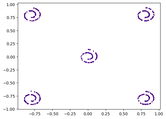
(a) Data

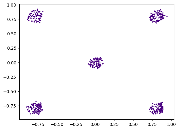
(b) VP

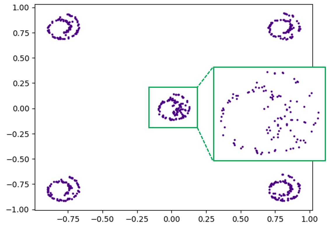
(c) CLD

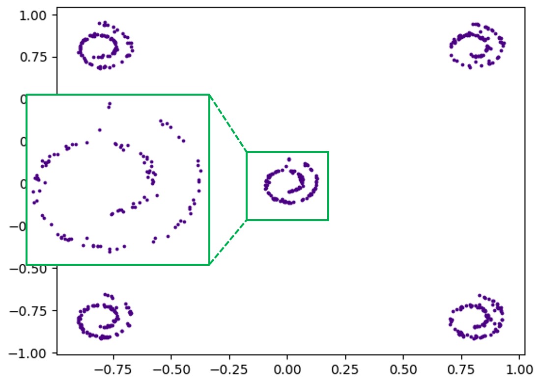
(d) HOLD

Figure 4: Comparison of 2D multi-Swiss rolls generated by three DGMs based on VP SDE, CLD and HOLD.

In the calculation process of $e^{\frac{t\mathcal{L}_{A}^{\dagger}}{2P}}$, the mean and variance after $\frac{t}{2P}$ time need to be calculated. By solving the generative HOLD (12), $e^{\mathcal{L}_{A}^{\dagger}\frac{t}{2P}}{\mathbf{x}}_{t}$ is a Gaussian distribution with mean ${\bm{\mu}}_{t}$ and variance ${\bm{\Sigma}}_{t}$ by integrating

$$\frac{d{\bm{\mu}}_{t}}{dt} ={\bm{l}}(t){\bm{\mu}}_{t},$$ (16)

$$\frac{d{\bm{\Sigma}}_{t}}{dt} ={\bm{l}}(t){\bm{\Sigma}}_{t}+\left[{\bm{l}}(t){\bm{\Sigma}}_{t}\right]^{\top}+{\bm{M}}(t){\bm{M}}(t)^{\top}.$$ (17)

over $[t,t+\frac{t}{2P}]$, where ${\bm{l}}(t)$ and ${\bm{M}}(t)$ are

$$\begin{pmatrix}0&-1&0\\ 1&0&-\sqrt{10}\\ 0&\sqrt{10}&-6\end{pmatrix}\otimes{\bm{I}}_{d},\quad\begin{pmatrix}0&0&0\\ 0&0&0\\ 0&0&\sqrt{12L^{-1}}\end{pmatrix}\otimes{\bm{I}}_{d},$$

respectively. Please refer to the App. 10.2 for the details of calculation process and results.

For the second operator $e^{\mathcal{L}_{B}^{\dagger}\frac{t}{P}}$, which involves a derivative with respect to acceleration variable acts on the ${\mathbf{x}}_{t}$ appearing in both components of the vector appearing on the right side of Eq. (14). We use one step Euler method to do the updating (solving) of Eq. (14). Whether it is step (13) or step (14), each iteration of the Lie-Trotter algorithm is accurate sampling, and the mixing speed of HOLD is also very fast, so the sampling algorithm can converge quickly, thus sampling at a fast speed. Experimental results in Section 6.2 also show the effectiveness of the Lie-Trotter method.

5 Image Restoration with HOLD

6 Experiments

Table 1: Unconditional CIFAR-10 generative performance.

Model	NLL$\downarrow$	FID$\downarrow$
HOLD-DGM (Prob. Flow) (ours)	$\leq$2.94	1.88
HOLD-DGM (SDE) (ours)	-	1.85
PFGM++ [Xu et al.(2023)Xu, Liu, Tian, Tong, Tegmark, and Jaakkola]	-	1.91
EDM [Karras et al.(2022)Karras, Aittala, Aila, and Laine]	-	1.97
CLD-SGM (Prob. Flow)	$\leq$3.31	2.25
CLD-SGM (SDE)	-	2.23
DDPM++, VPSDE (SDE) [Song et al.(2020b)Song, Sohl-Dickstein, Kingma, Kumar, Ermon, and Poole]	-	2.41
DDPM [Ho et al.(2020)Ho, Jain, and Abbeel]	$\leq$3.75	3.17
Likelihood SDE [Song et al.(2021)Song, Durkan, Murray, and Ermon]	2.84	2.87
DDIM (100 steps) [Song et al.(2020a)Song, Meng, and Ermon]	-	4.16
FastDDPM (100 steps) [Kong and Ping(2021)]	-	2.86
Improved DDPM [Nichol and Dhariwal(2021)]	3.37	2.90
UDM [Kim et al.(2021)Kim, Shin, Song, Kang, and Moon]	3.04	2.33
StyleGAN2 w/ ADA [Karras et al.(2020)Karras, Aittala, Hellsten, Laine, Lehtinen, and Aila]	-	2.92
Glow [Kingma and Dhariwal(2018)]	3.35	48.9
Residual Flow [Chen et al.(2019)Chen, Behrmann, Duvenaud, and Jacobsen]	3.28	46.37
DC-VAE [Parmar et al.(2021)Parmar, Li, Lee, and Tu]	-	17.90
VAEBM [Xiao et al.(2020)Xiao, Kreis, Kautz, and Vahdat]	-	12.2
Recovery EBM [Gao et al.(2020)Gao, Song, Poole, Wu, and Kingma]	3.18	9.58

HOLD-DGM is a general data generation model that can synthesize data of arbitrary modality. In order to verify its effectiveness, in this paper we use HOLD-DGM to generate a variety of image data. Similar to many generative models based on score and SDE, only one neural network $\mathfrak{S}_{\bm{\theta}}({\mathbf{x}}_{t},t)$ is needed in the whole system to predict the score. In this paper, we consistently use NCSN++ [Song and Ermon(2020), Song et al.(2021)Song, Durkan, Murray, and Ermon] with 9 input channels (for data, velocity, and acceleration) instead of 3 for $\mathfrak{S}_{\bm{\theta}}({\mathbf{x}}_{t},t)$.

From Section 3.1, it can be seen that HOLD-DGM does not have many hyperparameters, and in order to make the base of the mean and variance of the transition probability simple and elegant, several hyperparameters are fixed in all experiments, such as $\gamma{=}\sqrt{10}$ and $\xi{=}6$. In this way, the adjustable hyperparameters in the entire HOLD-DGM are only $\alpha$ (the variance scaling of the initial velocity and acceleration distribution) and $L$, except for the parameters in the neural network. All HOLD-DGM are trained under the proposed BCSM objective, and we found that as long as ${\mathbf{b}}_{0}$ is not equal to {${\mathbf{q}}_{0}$, ${\mathbf{p}}_{0}$, ${\mathbf{s}}_{0}$}, the basic performance is similar. We use ${\mathbf{b}}_{0}=\{{\mathbf{q}}_{0}\}$ in all experiments. The BCSM objective is used with the weighting $\lambda(t){=}(\ell^{BCSM}_{t})^{-2}$, which promotes image quality.

For the sampling algorithm, to highlight our proposed (Lie-Trotter) LT algorithm, we tried two other types of sampling algorithms, including (i) Probability flow using a Runge–Kutta method; reverse-time generative HOLD sampling using (ii) EM. For EM and LT, we use evaluation times chosen according to a quadratic function, like previous work [Kong and Ping(2021), Watson et al.(2021)Watson, Ho, Norouzi, and Chan].

In order to evaluate the quality of the images generated by the model trained on CIFAR-10, two metrics are used in this paper, one is FID with 50,000 samples [Heusel et al.(2017)Heusel, Ramsauer, Unterthiner, Nessler, and Hochreiter] and the other is negative log-likelihood (NLL). Similar to most SDE-based generative models, HOLD-DGM has no way to accurately calculate NLL, so this paper uses an upper bound to approximate. This upper bound is obtained by ${-}\log p({\mathbf{q}}_{0}){\leq}{-}\mathbb{E}_{{\mathbf{p}}_{0},{\mathbf{s}}_{0}\sim p({\mathbf{p}}_{0},{\mathbf{s}}_{0})}\log p_{\varepsilon}({\mathbf{q}}_{0},{\mathbf{p}}_{0},{\mathbf{s}}_{0}){-}H$ (refer App. 10.4 for derivation details), where $H$ is the entropy of $p({\mathbf{p}}_{0},{\mathbf{s}}_{0})$ and $\log p_{\varepsilon}({\mathbf{q}}_{0},{\mathbf{p}}_{0},{\mathbf{s}}_{0})$ is an unbiased estimate of $\log p({\mathbf{q}}_{0},{\mathbf{p}}_{0},{\mathbf{s}}_{0})$ from the probability flow ODE [Grathwohl et al.(2018)Grathwohl, Chen, Bettencourt, Sutskever, and Duvenaud, Song et al.(2020b)Song, Sohl-Dickstein, Kingma, Kumar, Ermon, and Poole] of HOLD. And since HOLD-DGM is not trained with the goal of minimizing NLL, its performance on NLL is not the best. This is a future work where we will try to train HOLD-DGM using maximum likelihood as the objective.

In order to compare the generation efficiency of different models, we also counted the number of function evaluations (NFEs, mainly score calculations), which is the most computationally resource-intensive part of the generation process.

We have done 1D data, 2D data, and high-dimensional data (image) generation experiments, and all experimental setting details are in App. 12. To save space, here we only introduce the effect for image generation.

6.1 2D multi-swiss roll generation

6.2 Image Generation

Similar to [Song and Ermon(2020)] and [Dockhorn et al.(2021)Dockhorn, Vahdat, and Kreis], we also conduct experiments on the widely used CIFAR-10 unconditional image generation benchmark for verification.

First of all, if the computing resource limitation during sampling is not considered, that is, there is no upper limit for NFE, we can achieve state-of-the-art performance. As shown in Table 1, when using HOLD ODE stream sampling, FID is 2.22, and when using reverse HOLD sampling, FID is 2.20. Although our NLL is not optimal, it is also in a very competitive position from the perspective of the upper bound [Dockhorn et al.(2021)Dockhorn, Vahdat, and Kreis, Vahdat et al.(2021)Vahdat, Kreis, and Kautz]. This shows that our HOLD-DGM generates data with no fewer modes than other best generative models. In the case of considering computation cost, i.e. under the same NFE budget and capacity of the model, our HOLD-DGM has a better performance than other models, as shown in Table 2. Due to the special form of HOLD, our proposed LT sampling algorithm has customized excellent performance. It can be seen that LT is much better than EM, and LT is also much better than SSCS algorithm proposed by [Dockhorn et al.(2021)Dockhorn, Vahdat, and Kreis]. Figure 5 shows some generated CIFAR-10 samples.

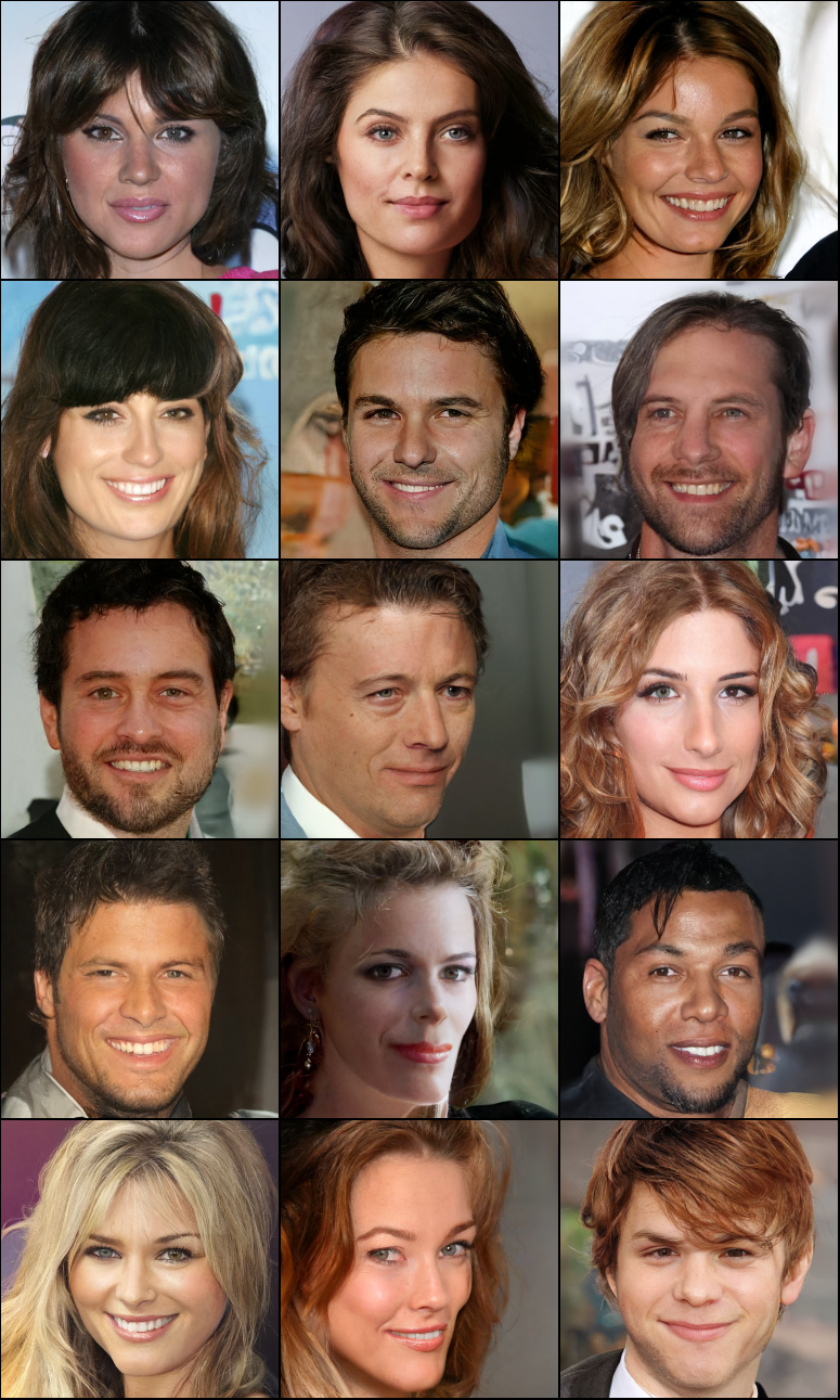
Figure 6: Generated CelebA-HQ-256 samples.

HOLD-DGM not only has very good performance on low-resolution CIFAR-10, but it can also synthesize high-resolution images. Figure 6 shows the images generated by HOLD-DGM after training on CelebA-HQ [Karras et al.(2018)Karras, Aila, Laine, and Lehtinen] with a resolution of $256\times 256$. It can be seen that our model is very good in terms of the authenticity and diversity (that is, coverage) of the faces. There are also more sample images in App. 12.3.

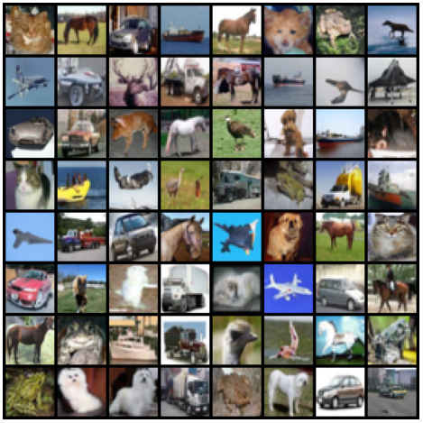
Figure 5: Generated CIFAR-10 samples without cherry-picking.

Table 2: Performance comparison under the same NFEs (Results other than HOLD come from [Dockhorn et al.(2021)Dockhorn, Vahdat, and Kreis]).

		FID at $n$ function evaluations $\downarrow$
Model	Sampler	$n{=}50$	$n{=}150$	$n{=}500$	$n{=}1000$	$n{=}2000$
HOLD	LT	15.1	2.67	2.07	1.96	1.85
HOLD	EM	38.2	5.60	2.24	2.18	2.12
CLD	SSCS	20.5	3.07	2.25	2.30	2.29
VPSDE	EM	28.2	4.06	2.47	2.66	2.60
VESDE	PC	460	216	3.75	2.43	2.23

6.3 Ablation Studies

We conducted ablation studies to prove that HOLD is very effective in DGM, and it is not sensitive to hyperparameters. The network configuration used here is the same as that used above. We did this research on three aspects in HOLD-DGM, namely the hyperparameters $L$ and $\alpha$ sampling algorithm. $L$ is mainly in the sub-equation of acceleration in HOLD (6), which is used to control the influence of Wiener process on acceleration. The smaller $L$ is, the greater the influence of Wiener process on acceleration, so that the inflow acceleration and speed will be faster. $\alpha$ is the initial velocity and acceleration variance scalings. Table 3 shows the performance of HOLD-DGM under different $L$ and $\alpha$. Intuitively, the results are not much different. But when $L$ is relatively small, the performance of FID will be better. The situation is very similar for $\alpha$, a small $\alpha$ will have slightly better performance. That is to say, at the beginning of data diffusion, the speed and acceleration should be set smaller, so that a better FID can be obtained

The experimental results also show that the performance of HOLD-DGM is not sensitive to hyperparameters $L$ and $\alpha$ , which is a good property and is easy to transplant to other generation tasks, such as 3D data.

Table 3: FID performance for different $L$ and $\alpha$.

FID$\downarrow$	$L=1.0$	$L=2.0$	$L=4.0$
$\alpha=0.02$	1.89	1.85	1.95
$\alpha=0.04$	1.92	1.90	1.93
$\alpha=0.08$	1.96	1.91	2.00

7 Conclusion

We introduce a new framework for score-based generative modeling with high-order Langevin dynamics. Our work enables a deep understanding of SDE-based approaches, decoupling of data and Wiener processes, smoother sampling path, flexible objective, sampling with higher expressiveness, and brings new possibilities to the family of generative models based on SDE and score matching.

Supplementary Material

8 A Lemma

We first introduce a lemma that will be used in some fact derivations in the following sections.

Lemma 1.

(Exponential of Kronecker product) Let ${\bm{A}}\in\mathbb{R}^{d\times d}$ and ${\bm{I}}$ is identity matrix, then $\exp({\bm{A}}\otimes{\bm{I}})=\exp({\bm{A}})\otimes{\bm{I}}$.

Proof.

First we have

$$\left({\bm{A}}\otimes{\bm{I}}\right)\left({\bm{A}}\otimes{\bm{I}}\right)=\begin{pmatrix}a_{11}{\bm{I}}&a_{12}{\bm{I}}&\dots&a_{1d}{\bm{I}}\\ a_{21}{\bm{I}}&a_{22}{\bm{I}}&\dots&x_{2n}{\bm{I}}\\ \vdots&\vdots&\vdots&\vdots\\ a_{d1}{\bm{I}}&a_{d2}{\bm{I}}&\dots&a_{dd}{\bm{I}}\end{pmatrix}\begin{pmatrix}a_{11}{\bm{I}}&a_{12}{\bm{I}}&\dots&a_{1d}{\bm{I}}\\ a_{21}{\bm{I}}&a_{22}{\bm{I}}&\dots&x_{2n}{\bm{I}}\\ \vdots&\vdots&\vdots&\vdots\\ a_{d1}{\bm{I}}&a_{d2}{\bm{I}}&\dots&a_{dd}{\bm{I}}\end{pmatrix}={\bm{A}}^{2}\otimes{\bm{I}}.$$

Then by induction on $n$, we obtain

$$\left({\bm{A}}\otimes{\bm{I}}\right)^{n}={\bm{A}}^{n}\otimes{\bm{I}}.$$

Therefore

$$\exp\left({\bm{A}}\otimes{\bm{I}}\right)=1+\sum_{n=1}^{\infty}\frac{\left({\bm{A}}\otimes{\bm{I}}\right)^{n}}{n!}=1+\sum_{n=1}^{\infty}\frac{{\bm{A}}^{n}\otimes{\bm{I}}}{n!}=1+\sum_{n=1}^{\infty}\frac{{\bm{A}}^{n}}{n!}\otimes{\bm{I}}=\exp({\bm{A}})\otimes{\bm{I}}.$$

∎

9 High-Order Langevin Dynamics

A pair of general linear forward diffusion and backward SDE is

$$d{\mathbf{x}}_{t} ={\bm{f}}(t){\mathbf{x}}_{t}\,dt+{\bm{G}}(t)\,d{\mathbf{w}}_{t},\quad t\in[0,T]$$ (18)

and

$$d{\mathbf{x}}_{t} =\left[-{\bm{f}}(t){\mathbf{x}}_{t}+{\bm{G}}(t){\bm{G}}(t)^{\top}\nabla_{{\mathbf{x}}_{t}}\log p_{t}({\mathbf{x}}_{t})\right]\,dt+{\bm{G}}(t)d\bar{\mathbf{w}}_{t},$$ (19)

where ${\bm{f}}(t),{\bm{G}}(t)\in\mathbb{R}^{3d\times 3d}$, ${\mathbf{w}}_{t}$ is the standard Wiener process, and $\bar{\mathbf{w}}_{t}$ is time-reverse Wiener process. Recall that the High-order (third-order) Langevin dynamics (HOLD) in the main paper is

$$\begin{split}d{\mathbf{q}}_{t}&={\mathbf{p}}_{t}dt,\\ d{\mathbf{p}}_{t}&=-mL^{-1}{\mathbf{q}}_{t}dt+\gamma{\mathbf{s}}_{t}dt,\\ d{\mathbf{s}}_{t}&=-\gamma{\mathbf{p}}_{t}dt-\xi{\mathbf{s}}_{t}dt+\sqrt{2\xi L^{-1}}d{\mathbf{w}}_{t}.\end{split}$$ (20)

We can write it in matrix form as Eq. (18), and it is

$$\begin{pmatrix}d{\mathbf{q}}_{t}\\ d{\mathbf{p}}_{t}\\ d{\mathbf{s}}_{t}\end{pmatrix}=\begin{pmatrix}{\mathbf{p}}_{t}\\ -mL^{-1}{\mathbf{q}}_{t}\\ \bm{0}_{d}\end{pmatrix}dt+\begin{pmatrix}\bm{0}_{d}\\ \gamma{\mathbf{s}}_{t}\\ -\gamma{\mathbf{p}}_{t}\end{pmatrix}dt+\begin{pmatrix}\bm{0}_{d}\\ \bm{0}_{d}\\ -\xi{\mathbf{s}}_{t}\end{pmatrix}dt+\begin{pmatrix}\bm{0}_{d}\\ \bm{0}_{d}\\ \sqrt{2\xi L^{-1}}d{\mathbf{w}}_{t}\end{pmatrix}.$$ (21)

Let ${\mathbf{x}}_{t}=({\mathbf{q}}_{t},{\mathbf{p}}_{t},{\mathbf{s}}_{t})^{\top}\in\mathbb{R}^{3d}$, then we have

$${\bm{f}}(t)\coloneqq\begin{pmatrix}0&1&0\\ -mL^{-1}&0&\gamma\\ 0&-\gamma&-\xi\end{pmatrix}\otimes{\bm{I}}_{d},\qquad{\bm{G}}(t)\coloneqq\begin{pmatrix}0&0&0\\ 0&0&0\\ 0&0&\sqrt{2\xi L^{-1}}\end{pmatrix}\otimes{\bm{I}}_{d},$$ (22)

where $\otimes$ denotes the Kronecker product. For the simplicity and elegance of the calculation, in this paper we set $m=L$, $\xi=6$, and $\gamma=\sqrt{10}$ then the HOLD (20) is simplified into Eq. (18) with

$${\bm{f}}(t)\coloneqq\begin{pmatrix}0&1&0\\ -1&0&\sqrt{10}\\ 0&-\sqrt{10}&-6\end{pmatrix}\otimes{\bm{I}}_{d},\qquad{\bm{G}}(t)\coloneqq\begin{pmatrix}0&0&0\\ 0&0&0\\ 0&0&\sqrt{12L^{-1}}\end{pmatrix}\otimes{\bm{I}}_{d}.$$ (23)

9.1 Perturbation Kernel

For linear SDE, we can get the score by solving an associated deterministic ordinary differential equation. The transition densities $p({\mathbf{x}}_{t}|{\mathbf{x}}_{0})$ of the solution process ${\mathbf{x}}_{t}$ for the SDE (20) is the solution to the Fokker-Planck-Kolmogorov (FPK) equation [Särkkä and Solin(2019)]

$$\frac{\partial p({\mathbf{x}}_{t},t)}{\partial t}=-\sum_{i=1}^{d}\frac{\partial\left[({\bm{f}}(t){\mathbf{x}}_{t})_{i}p({\mathbf{x}}_{t},t)\right]}{\partial x_{i}}+\sum_{i=1}^{d}\sum_{j=1}^{d}\frac{\partial^{2}}{\partial x_{i}\partial x_{j}}[({\bm{G}}(t){\bm{G}}(t)^{\top})_{i,j}p({\mathbf{x}}_{t},t)],$$ (24)

where $({\bm{f}}(t){\mathbf{x}}_{t})_{i}$ is the $i$-th element of the vector ${\bm{f}}(t){\mathbf{x}}_{t}$, and $({\bm{G}}(t){\bm{G}}(t)^{\top})_{i,j}$ is the element in the $i$-th row and $j$-th column of the matrix ${\bm{G}}(t){\bm{G}}(t)^{\top}$. Thus in this case we can derive that $p(\mathbf{x}(t)|\mathbf{x}(0))$ is Gaussian with mean ${\bm{\mu}}_{t}$ and variance ${\bm{\Sigma}}_{t}$ satisfy the following ordinary differential equations (ODEs) [Särkkä and Solin(2019)]

$$\frac{d{\bm{\mu}}_{t}}{dt} ={\bm{f}}(t){\bm{\mu}}_{t},$$ (25)

$$\frac{d{\bm{\Sigma}}_{t}}{dt} ={\bm{f}}(t){\bm{\Sigma}}_{t}+\left[{\bm{f}}(t){\bm{\Sigma}}_{t}\right]^{\top}+{\bm{G}}(t){\bm{G}}(t)^{\top}.$$ (26)

This array of ODE is easy to solve, and we have

$${\bm{\mu}}_{t} =\exp\left[\int_{0}^{t}{\bm{f}}(\tau)d\tau\right]{\bm{\mu}}_{0},$$ (27)

$${\bm{\Sigma}}_{t} =\exp\left[\int_{0}^{t}{\bm{f}}(\tau)d\tau\right]{\bm{\Sigma}}_{0}\exp\left[\int_{0}^{t}{\bm{f}}(\tau)d\tau\right]^{\top}+\int_{0}^{t}\exp\left[\int_{s}^{t}{\bm{f}}(\tau)d\tau\right]{\bm{G}}(s){\bm{G}}(s)^{\top}\exp\left[\int_{s}^{t}{\bm{f}}(\tau)d\tau\right]^{\top}ds$$ (28)

where

$$\int_{0}^{t}{\bm{f}}(\tau)d\tau=t\begin{pmatrix}0&1&0\\ -1&0&\sqrt{10}\\ 0&-\sqrt{10}&-6\end{pmatrix}\otimes{\bm{I}}_{d}.$$ (29)

Let ${\bm{F}}=\begin{pmatrix}0&1&0\\ -1&0&\sqrt{10}\\ 0&-\sqrt{10}&-6\end{pmatrix}$, then the eigenvalues of ${\bm{F}}$ are $-3$, $-2$, and $-1$. By the Putzer’s spectral formula [Putzer(1966)] and Lemma 1 we have

$$\exp\left[\int_{0}^{t}{\bm{f}}(\tau)d\tau\right]=\exp(t{\bm{F}}\otimes{\bm{I}}_{d})=\left[r_{1}(t){\bm{P}}_{1}+r_{2}(t){\bm{P}}_{2}+r_{3}(t){\bm{P}}_{3}\right]\otimes{\bm{I}}_{d},$$ (30)

where

$${\bm{P}}_{1}={\bm{I}},\quad{\bm{P}}_{2}=({\bm{F}}+3{\bm{I}}){\bm{P}}_{1},\quad{\bm{P}}_{3}=({\bm{F}}+2{\bm{I}}){\bm{P}}_{2},$$ (31)

and

$$r^{\prime}_{1}(t)=-3r_{1}(t),\quad r_{1}(0)=1,$$ (32)

$$r^{\prime}_{2}(t)=-2r_{2}(t)+r_{1}(t),\quad r_{2}(0)=0,$$ (33)

$$r^{\prime}_{3}(t)=-r_{3}(t)+r_{2}(t),\quad r_{3}(0)=0.$$ (34)

By integration of these ODEs, therefore

$$\begin{split}&{\bm{P}}_{1}={\bm{I}},\quad{\bm{P}}_{2}=\begin{pmatrix}3&1&0\\ -1&3&\sqrt{10}\\ 0&-\sqrt{10}&-3\end{pmatrix},\quad{\bm{P}}_{3}=\begin{pmatrix}5&5&\sqrt{10}\\ -5&-5&-\sqrt{10}\\ \sqrt{10}&\sqrt{10}&2\end{pmatrix},\end{split}$$ (35)

and

$$\begin{split}&r_{1}(t)=\exp\left(-3t\right),\quad r_{2}(t)=\exp\left(-2t\right)-\exp\left(-3t\right),\\ &r_{3}(t)=\frac{1}{2}\exp\left(-t\right)+\frac{1}{2}\exp\left(-3t\right)-\exp\left(-2t\right).\end{split}$$ (36)

Plugging (35) and (36) into (30), and by direct calculation we obtain the elements of $\exp(t{\bm{F}})$ are

$$f_{11}(t)=\frac{5}{2}\exp(-t)-2\exp(-2t)+\frac{1}{2}\exp(-3t),$$ (37)

$$f_{12}(t)=\frac{5}{2}\exp(-t)-4\exp(-2t)+\frac{3}{2}\exp(-3t),$$ (38)

$$f_{13}(t)=\sqrt{10}\left[\frac{1}{2}\exp\left(-t\right)-\exp\left(-2t\right)+\frac{1}{2}\exp\left(-3t\right)\right],$$ (39)

$$f_{21}(t)=-\frac{5}{2}\exp(-t)+4\exp(-2t)-\frac{3}{2}\exp(-3t),$$ (40)

$$f_{22}(t)=-\frac{5}{2}\exp(-t)+8\exp(-2t)-\frac{9}{2}\exp(-3t),$$ (41)

$$f_{23}(t)=\sqrt{10}\left[-\frac{1}{2}\exp\left(-t\right)+2\exp\left(-2t\right)-\frac{3}{2}\exp\left(-3t\right)\right],$$ (42)

$$f_{31}(t)=\sqrt{10}\left[\frac{1}{2}\exp\left(-t\right)-\exp\left(-2t\right)+\frac{1}{2}\exp\left(-3t\right)\right],$$ (43)

$$f_{32}(t)=\sqrt{10}\left[\frac{1}{2}\exp\left(-t\right)-2\exp\left(-2t\right)+\frac{3}{2}\exp\left(-3t\right)\right],$$ (44)

$$f_{33}(t)=\exp(-t)-5\exp(-2t)+5\exp(-3t).$$ (45)

Let ${\bm{\mu}}_{0}=({\mathbf{q}}_{0},{\mathbf{p}}_{0},{\mathbf{s}}_{0})^{\top}$, thus the mean is

$${\bm{\mu}}_{t}=\begin{pmatrix}f_{11}(t){\mathbf{q}}_{0}+f_{12}(t){\mathbf{p}}_{0}+f_{13}(t){\mathbf{s}}_{0}\\ f_{21}(t){\mathbf{q}}_{0}+f_{22}(t){\mathbf{p}}_{0}+f_{23}(t){\mathbf{s}}_{0}\\ f_{31}(t){\mathbf{q}}_{0}+f_{32}(t){\mathbf{p}}_{0}+f_{33}(t){\mathbf{s}}_{0}\end{pmatrix}.$$ (46)

For the variance, let ${\bm{\Sigma}}_{0}=\mathrm{diag}(\Sigma_{0}^{qq},\Sigma_{0}^{pp},\Sigma_{0}^{ss})\otimes{\bm{I}}_{d}$, plugging the formula of $\exp(t{\bm{F}})$ (Eq. (30)) into ${\bm{\Sigma}}_{t}$ (Eq. (28)), implies that ${\bm{\Sigma}}_{t}$ equals

$$\exp\left[\int_{0}^{t}{\bm{f}}(\tau)d\tau\right]{\bm{\Sigma}}_{0}\exp\left[\int_{0}^{t}{\bm{f}}(\tau)d\tau\right]^{\top}+\int_{0}^{t}\exp\left[\int_{s}^{t}{\bm{f}}(\tau)d\tau\right]{\bm{G}}(s){\bm{G}}(s)^{\top}\exp\left[\int_{s}^{t}{\bm{f}}(\tau)d\tau\right]^{\top}ds$$ (47)

$$=\left[\begin{pmatrix}f_{11}(t)&f_{12}(t)&f_{13}(t)\\ f_{21}(t)&f_{22}(t)&f_{23}(t)\\ f_{31}(t)&f_{32}(t)&f_{33}(t)\end{pmatrix}\begin{pmatrix}\Sigma_{0}^{qq}&0&0\\ 0&\Sigma_{0}^{pp}&0\\ 0&0&\Sigma_{0}^{ss}\end{pmatrix}\begin{pmatrix}f_{11}(t)&f_{12}(t)&f_{13}(t)\\ f_{21}(t)&f_{22}(t)&f_{23}(t)\\ f_{31}(t)&f_{32}(t)&f_{33}(t)\end{pmatrix}^{\top}\right]\otimes{\bm{I}}_{d}$$ (48)

$$+\int_{0}^{t}\left[\begin{pmatrix}f_{11}(t-s)&f_{12}(t-s)&f_{13}(t-s)\\ f_{21}(t-s)&f_{22}(t-s)&f_{23}(t-s)\\ f_{31}(t-s)&f_{32}(t-s)&f_{33}(t-s)\end{pmatrix}\begin{pmatrix}0&0&0\\ 0&0&0\\ 0&0&12L^{-1}\end{pmatrix}\begin{pmatrix}f_{11}(t-s)&f_{12}(t-s)&f_{13}(t-s)\\ f_{21}(t-s)&f_{22}(t-s)&f_{23}(t-s)\\ f_{31}(t-s)&f_{32}(t-s)&f_{33}(t-s)\end{pmatrix}^{\top}\right]\otimes{\bm{I}}_{d}ds$$ (49)

$$=\begin{pmatrix}\sum_{j=1}^{3}f_{1j}^{2}(t)\Sigma_{0}^{jj}&\sum_{j=1}^{3}f_{1j}(t)f_{2j}(t)\Sigma_{0}^{jj}&\sum_{j=1}^{3}f_{1j}(t)f_{3j}(t)\Sigma_{0}^{jj}\\ \sum_{j=1}^{3}f_{2j}(t)f_{1j}(t)\Sigma_{0}^{jj}&\sum_{j=1}^{3}f_{2j}^{2}(t)\Sigma_{0}^{jj}&\sum_{j=1}^{3}f_{2j}(t)f_{3j}(t)\Sigma_{0}^{jj}\\ \sum_{j=1}^{3}f_{3j}(t)f_{1j}(t)\Sigma_{0}^{jj}&\sum_{j=1}^{3}f_{3j}(t)f_{2j}(t)\Sigma_{0}^{jj}&\sum_{j=1}^{3}f_{3j}^{2}(t)\Sigma_{0}^{jj}\end{pmatrix}\otimes{\bm{I}}_{d}$$ (50)

$$+12L^{-1}\int_{0}^{t}\begin{pmatrix}f_{13}^{2}(t-s)&f_{13}(t-s)f_{23}(t-s)&f_{13}(t-s)f_{33}(t-s)\\ f_{23}(t-s)f_{13}(t-s)&f_{23}^{2}(t-s)&f_{23}(t-s)f_{33}(t-s)\\ f_{33}(t-s)f_{13}(t-s)&f_{33}(t-s)f_{23}(t-s)&f_{33}^{2}(t-s)\end{pmatrix}ds\otimes{\bm{I}}_{d}$$ (51)

where we let $1\leftrightarrow q,2\leftrightarrow p,3\leftrightarrow s$ in $\Sigma_{0}^{jj}$ to simplify notation. On the other hand we have

$${\bm{\Sigma}}_{t}=\Sigma_{t}\otimes{\bm{I}}_{d},\quad\Sigma_{t}=\begin{pmatrix}\Sigma_{t}^{qq}&\Sigma_{t}^{qp}&\Sigma_{t}^{qs}\\ \Sigma_{t}^{qp}&\Sigma_{t}^{pp}&\Sigma_{t}^{ps}\\ \Sigma_{t}^{qs}&\Sigma_{t}^{ps}&\Sigma_{t}^{ss}\end{pmatrix},$$ (52)

which clearly implies that

$$\Sigma_{t}^{qq}=\sum_{j=1}^{3}f_{1j}^{2}(t)\Sigma_{0}^{jj}+12L^{-1}\int_{0}^{t}f_{13}^{2}(t-s)ds,$$ (53)

$$\Sigma_{t}^{qp}=\sum_{j=1}^{3}f_{1j}(t)f_{2j}(t)\Sigma_{0}^{jj}+12L^{-1}\int_{0}^{t}f_{13}(t-s)f_{23}(t-s)ds,$$ (54)

$$\Sigma_{t}^{qs}=\sum_{j=1}^{3}f_{1j}(t)f_{3j}(t)\Sigma_{0}^{jj}+12L^{-1}\int_{0}^{t}f_{13}(t-s)f_{33}(t-s)ds,$$ (55)

$$\Sigma_{t}^{pp}=\sum_{j=1}^{3}f_{2j}^{2}(t)\Sigma_{0}^{jj}+12L^{-1}\int_{0}^{t}f_{23}^{2}(t-s)ds,$$ (56)

$$\Sigma_{t}^{ps}=\sum_{j=1}^{3}f_{2j}(t)f_{3j}(t)\Sigma_{0}^{jj}+12L^{-1}\int_{0}^{t}f_{23}(t-s)f_{33}(t-s)ds,$$ (57)

$$\Sigma_{t}^{ss}=\sum_{j=1}^{3}f_{3j}^{2}(t)\Sigma_{0}^{jj}+12L^{-1}\int_{0}^{t}f_{33}^{2}(t-s)ds,$$ (58)

where

$$f_{13}^{2}(t)=f_{31}^{2}(t)=\frac{5}{2}\exp(-2t)-10\exp(-3t)+15\exp(-4t)-10\exp(-5t)+\frac{5}{2}\exp(-6t),$$ (59)

$$f_{23}^{2}(t)=f_{32}^{2}(t)=\frac{5}{2}\exp(-2t)-20\exp(-3t)+55\exp(-4t)-60\exp(-5t)+\frac{45}{2}\exp(-6t),$$ (60)

$$f_{33}^{2}(t)=\exp(-2t)-10\exp(-3t)+35\exp(-4t)-50\exp(-5t)+25\exp(-6t),$$ (61)

$$f_{13}(t)f_{23}(t)=-\frac{5}{2}\exp(-2t)+15\exp(-3t)-30\exp(-4t)+25\exp(-5t)-\frac{15}{2}\exp(-6t),$$ (62)

$$f_{13}(t)f_{33}(t)=\frac{\sqrt{10}}{2}\exp(-2t)-\frac{7\sqrt{10}}{2}\exp(-3t)+8\sqrt{10}\exp(-4t)-\frac{15\sqrt{10}}{2}\exp(-5t)+\frac{5\sqrt{10}}{2}\exp(-6t),$$ (63)

$$f_{23}(t)f_{33}(t)=\sqrt{10}\left[-\frac{1}{2}\exp(-2t)+\frac{9}{2}\exp(-3t)-14\exp(-4t)+\frac{35}{2}\exp(-5t)-\frac{15}{2}\exp(-6t)\right],$$ (64)

$$f_{11}^{2}(t)=\frac{25}{4}\exp(-2t)-10\exp(-3t)+\frac{13}{2}\exp(-4t)-2\exp(-5t)+\frac{1}{4}\exp(-6t),$$ (65)

$$f_{12}^{2}(t)=f_{21}^{2}(t)=\frac{25}{4}\exp(-2t)-20\exp(-3t)+\frac{47}{2}\exp(-4t)-12\exp(-5t)+\frac{9}{4}\exp(-6t),$$ (66)

$$f_{22}^{2}(t)=\frac{25}{4}\exp(-2t)-40\exp(-3t)+86.5\exp(-4t)-72\exp(-5t)+\frac{81}{4}\exp(-6t),$$ (67)

$$f_{21}(t)f_{31}(t)=-\frac{5\sqrt{10}}{4}\exp(-2t)+\frac{9\sqrt{10}}{2}\exp(-3t)-6\sqrt{10}\exp(-4t)+\frac{7\sqrt{10}}{2}\exp(-5t)-\frac{3\sqrt{10}}{4}\exp(-6t),$$ (68)

$$f_{22}(t)f_{32}(t)=\sqrt{10}\left[-\frac{5}{4}\exp(-2t)+9\exp(-3t)-22\exp(-4t)+21\exp(-5t)-\frac{27}{4}\exp(-6t)\right],$$ (69)

$$f_{11}(t)f_{31}(t)=\frac{5\sqrt{10}}{4}\exp(-2t)-\frac{7\sqrt{10}}{2}\exp(-3t)+\frac{7\sqrt{10}}{2}\exp(-4t)-\frac{3\sqrt{10}}{2}\exp(-5t)+\frac{\sqrt{10}}{4}\exp(-6t),$$ (70)

$$f_{12}(t)f_{32}(t)=\frac{5\sqrt{10}}{4}\exp(-2t)-7\sqrt{10}\exp(-3t)+\frac{25\sqrt{10}}{2}\exp(-4t)-9\sqrt{10}\exp(-5t)+\frac{9\sqrt{10}}{4}\exp(-6t),$$ (71)

$$f_{11}(t)f_{21}(t)=-\frac{25}{4}\exp(-2t)+15\exp(-3t)-13\exp(-4t)+5\exp(-5t)-\frac{3}{4}\exp(-6t),$$ (72)

$$f_{12}(t)f_{22}(t)=-\frac{25}{4}\exp(-2t)+30\exp(-3t)-47\exp(-4t)+30\exp(-5t)-\frac{27}{4}\exp(-6t).$$ (73)

Due to the fact $\int_{0}^{t}\exp(-a(t-s))ds=\frac{1-\exp(-at)}{a}$, so we can deduce that $\lim_{t\rightarrow\infty}\int_{0}^{t}\exp(-a(t-s))ds=\frac{1}{a}$. Then by direct computation we have

$$\lim_{t\rightarrow\infty}\Sigma^{qq}_{t} =2\xi L^{-1}\frac{1}{12}=L^{-1},$$ (74)

$$\lim_{t\rightarrow\infty}\Sigma^{pp}_{t} =2\xi L^{-1}\frac{1}{12}=L^{-1},$$ (75)

$$\lim_{t\rightarrow\infty}\Sigma^{ss}_{t} =2\xi L^{-1}\frac{1}{12}=L^{-1},$$ (76)

$$\lim_{t\rightarrow\infty}\Sigma^{qp}_{t} =0,$$ (77)

$$\lim_{t\rightarrow\infty}\Sigma^{qs}_{t} =0,$$ (78)

$$\lim_{t\rightarrow\infty}\Sigma^{ps}_{t} =0,$$ (79)

$$\lim_{t\rightarrow\infty}{\bm{\mu}}_{t} =\bm{0}_{3d},$$ (80)

which establishes the prior probability $p_{\infty}({\mathbf{x}})=\mathcal{N}({\mathbf{q}};\bm{0}_{d},L^{-1}{\bm{I}}_{d})\,\mathcal{N}({\mathbf{p}};\bm{0}_{d},L^{-1}{\bm{I}}_{d})\,\mathcal{N}({\mathbf{s}};\bm{0}_{d},L^{-1}{\bm{I}}_{d})$.

9.2 The Objective

Let $p({\mathbf{x}}_{0},0)$ denotes the distribution of target data (image, video, or audio etc. with initial velocity and acceleration) that we want to generate, and $p({\mathbf{x}}_{0},0)$ can be diffused through $p({\mathbf{x}}_{t},t)$ (sometimes it is abbreviated as $p_{t}$ for brevity) into $p({\mathbf{x}}_{T},T)$ by HOLD (Eq. (20)). The target of generation is to build a model to reverse this process, that is use time-reverse HOLD with Eq. (22) to sample from $q({\mathbf{x}}_{T},T)$ (approximation of the prior probability) and denoise it through $q({\mathbf{x}}_{t},t)$ into $q({\mathbf{x}}_{0},0)$. Thus our goal (or objective) is to make the difference between $q({\mathbf{x}}_{0},0)$ and $p({\mathbf{x}}_{0},0)$ as small as possible. Kullback–Leibler (KL) divergence is an effective measure to fulfil by

$$\begin{split}D_{\mathrm{KL}}(p_{0}\;\|\;q_{0})&=D_{\mathrm{KL}}(p_{0}\;\|\;q_{0})-D_{\mathrm{KL}}(p_{T}\;\|\;q_{T})+D_{\mathrm{KL}}(p_{T}\;\|\;q_{T})\\ &=-\int_{0}^{T}\frac{\partial D_{\mathrm{KL}}(p_{t}\;\|\;q_{t})}{\partial t}dt+D_{\mathrm{KL}}(p_{T}\;\|\;q_{T}).\end{split}$$ (81)

If $T$ is large, $D_{\mathrm{KL}}(p_{T}\;\|\;q_{T})$ is small enough to be ignored, so the most important thing to calculate an objective is to know the value of $\int_{0}^{T}\frac{\partial D_{\mathrm{KL}}(p_{t}\;\|\;q_{t})}{\partial t}dt$, whose deduction needs $\frac{\partial p({\mathbf{x}}_{t},t)}{\partial t}$, which can be obtained by the Fokker–Planck equation associated with our diffusion HOLD

$$\begin{split}\frac{\partial p({\mathbf{x}}_{t},t)}{\partial t}&=\nabla_{{\mathbf{x}}}\cdot\left[\tfrac{1}{2}\left({\bm{G}}(t){\bm{G}}(t)^{\top}\otimes{\bm{I}}_{d}\right)\nabla_{{\mathbf{x}}}p({\mathbf{x}}_{t},t)-p({\mathbf{x}}_{t},t)({\bm{f}}(t)\otimes{\bm{I}}_{d}){\mathbf{x}}_{t}\right]\\ &=\nabla_{{\mathbf{x}}_{t}}\cdot\left[{\bm{h}}_{p}({\mathbf{x}}_{t},t)p({\mathbf{x}}_{t},t)\right],\quad{\bm{h}}_{p}({\mathbf{x}}_{t},t)\coloneqq\tfrac{1}{2}\left({\bm{G}}(t){\bm{G}}(t)^{\top}\otimes{\bm{I}}_{d}\right)\nabla_{{\mathbf{x}}}\log p({\mathbf{x}}_{t},t)-({\bm{f}}(t)\otimes{\bm{I}}_{d}){\mathbf{x}}_{t},\end{split}$$ (82)

where $\nabla_{{\mathbf{x}}_{t}}\cdot$ is divergence, and $\nabla_{{\mathbf{x}}_{t}}$ is gradient. Then with Gauss’s theorem, we have

$$\begin{split}&\quad\frac{\partial D_{\mathrm{KL}}(p_{t}\;\|\;q_{t})}{\partial t}=\frac{\partial}{\partial t}\int p({\mathbf{x}}_{t},t)\log\frac{p({\mathbf{x}}_{t},t)}{q({\mathbf{x}}_{t},t)}\,d{\mathbf{x}}_{t}\\ &=\int\frac{\partial p({\mathbf{x}}_{t},t)}{\partial t}\log\frac{p({\mathbf{x}}_{t},t)}{q({\mathbf{x}}_{t},t)}+p({\mathbf{x}}_{t},t)\frac{\partial\log\frac{p({\mathbf{x}}_{t},t)}{q({\mathbf{x}}_{t},t)}}{\partial t}\,d{\mathbf{x}}_{t}\\ &=\int\nabla_{{\mathbf{x}}_{t}}\cdot\left[{\bm{h}}_{p}({\mathbf{x}}_{t},t)p({\mathbf{x}}_{t},t)\right]\left[\log{p({\mathbf{x}}_{t},t)}-\log{q({\mathbf{x}}_{t},t)}\right]+\frac{\partial p({\mathbf{x}}_{t},t)}{\partial t}-\frac{p({\mathbf{x}}_{t},t)}{q({\mathbf{x}}_{t},t)}\frac{\partial q({\mathbf{x}}_{t},t)}{\partial t}\,d{\mathbf{x}}_{t}\\ &=\int\left[{\bm{h}}_{p}({\mathbf{x}}_{t},t)p({\mathbf{x}}_{t},t)\right]\nabla\left[\log{p({\mathbf{x}}_{t},t)}-\log{q({\mathbf{x}}_{t},t)}\right]+\nabla_{{\mathbf{x}}_{t}}\cdot\left[{\bm{h}}_{p}({\mathbf{x}}_{t},t)p({\mathbf{x}}_{t},t)\right]-\frac{p({\mathbf{x}}_{t},t)}{q({\mathbf{x}}_{t},t)}\nabla_{{\mathbf{x}}_{t}}\cdot\left[{\bm{h}}_{q}({\mathbf{x}}_{t},t)q({\mathbf{x}}_{t},t)\right]\,d{\mathbf{x}}_{t}\\ &=\int-\left[{\bm{h}}_{p}({\mathbf{x}}_{t},t)p({\mathbf{x}}_{t},t)\right]^{\top}\nabla\left[\log{p({\mathbf{x}}_{t},t)}-\log{q({\mathbf{x}}_{t},t)}\right]+\left[{\bm{h}}_{q}({\mathbf{x}}_{t},t)q({\mathbf{x}}_{t},t)\right]^{\top}\nabla_{{\mathbf{x}}_{t}}\frac{p({\mathbf{x}}_{t},t)}{q({\mathbf{x}}_{t},t)}\,d{\mathbf{x}}_{t}\\ &=\int-\left[{\bm{h}}_{p}({\mathbf{x}}_{t},t)p({\mathbf{x}}_{t},t)\right]^{\top}\nabla\left[\log{p({\mathbf{x}}_{t},t)}-\log{q({\mathbf{x}}_{t},t)}\right]+\left[{\bm{h}}_{q}({\mathbf{x}}_{t},t)q({\mathbf{x}}_{t},t)\right]^{\top}\frac{q({\mathbf{x}}_{t},t)\nabla_{{\mathbf{x}}_{t}}p({\mathbf{x}}_{t},t)-p({\mathbf{x}}_{t},t)\nabla_{{\mathbf{x}}_{t}}q({\mathbf{x}}_{t},t)}{q^{2}({\mathbf{x}}_{t},t)}\,d{\mathbf{x}}_{t}\\ &=-\int p({\mathbf{x}}_{t},t)\left[{\bm{h}}_{p}({\mathbf{x}}_{t},t)-{\bm{h}}_{q}({\mathbf{x}}_{t},t)\right]^{\top}\left[\nabla_{{\mathbf{x}}_{t}}\log p({\mathbf{x}}_{t},t)-\nabla_{{\mathbf{x}}_{t}}\log q({\mathbf{x}}_{t},t)\right]\,d{\mathbf{x}}_{t}\\ &=-\frac{1}{2}\int p({\mathbf{x}}_{t},t)\left[\nabla_{{\mathbf{x}}_{t}}\log p({\mathbf{x}}_{t},t)-\nabla_{{\mathbf{x}}_{t}}\log q({\mathbf{x}}_{t},t)\right]^{\top}\left(G(t)G(t)^{\top}\otimes{\bm{I}}_{d}\right)[\nabla_{{\mathbf{x}}_{t}}\log p({\mathbf{x}}_{t},t)-\nabla_{{\mathbf{x}}_{t}}\log q({\mathbf{x}}_{t},t)]\,d{\mathbf{x}}_{t}\\ &=-6L^{-1}\int p({\mathbf{x}}_{t},t)\norm{\nabla_{{\mathbf{s}}_{t}}\log p({\mathbf{x}}_{t},t)-\nabla_{{\mathbf{s}}_{t}}\log q({\mathbf{x}}_{t},t)}_{2}^{2}\,d{\mathbf{x}}_{t}.\end{split}$$ (83)

Thus the objective is

$$\begin{split}D_{\mathrm{KL}}(p_{0}\;\|\;q_{0})&=\mathbb{E}_{t\sim{\mathcal{U}}[0,T],{\mathbf{x}}_{t}\sim p({\mathbf{x}},t)}\left[6L^{-1}\norm{\nabla_{{\mathbf{s}}_{t}}\log p({\mathbf{x}}_{t},t)-\nabla_{{\mathbf{s}}_{t}}\log q({\mathbf{x}}_{t},t)}_{2}^{2}\right]+D_{\mathrm{KL}}(p_{T}\;\|\;q_{T})\\ &\approx\mathbb{E}_{t\sim{\mathcal{U}}[0,T],{\mathbf{x}}_{t}\sim p({\mathbf{x}},t)}\left[6L^{-1}\norm{\nabla_{{\mathbf{s}}_{t}}\log p({\mathbf{x}}_{t},t)-\nabla_{{\mathbf{s}}_{t}}\log q({\mathbf{x}}_{t},t)}_{2}^{2}\right]\\ &=\mathbb{E}_{t\sim{\mathcal{U}}[0,T],{\mathbf{x}}_{t}\sim p({\mathbf{x}},t)}\left[\lambda(t)\norm{\nabla_{{\mathbf{s}}_{t}}\log p({\mathbf{x}}_{t},t)-\nabla_{{\mathbf{s}}_{t}}\log q({\mathbf{x}}_{t},t)}_{2}^{2}\right],\end{split}$$ (84)

where a more general objective function can be obtained by replacing $6L^{-1}$ with an arbitrary function $\lambda(t)$.

9.3 Denoising Score Matching and Hybrid Score Matching

In this work, a neural network is used to estimate the score $\nabla_{{\mathbf{s}}_{t}}\log p({\mathbf{x}}_{t},t)$. Let $\mathfrak{S}_{\bm{\theta}}({\mathbf{x}}_{t},t)$ denotes this score model. Substituting $\mathfrak{S}_{\bm{\theta}}({\mathbf{x}}_{t},t)$ for $\nabla_{{\mathbf{s}}_{t}}\log q({\mathbf{x}}_{t},t)$ in Eq. (84) gives the score matching (SM) loss

$${\mathcal{L}}_{\mathrm{SM}}\coloneqq\mathbb{E}_{t\sim{\mathcal{U}}[0,T]}\left[\lambda(t)\mathbb{E}_{{\mathbf{x}}_{t}\sim p({\mathbf{x}},t)}[\norm{\nabla_{{\mathbf{s}}_{t}}\log p({\mathbf{x}}_{t},t)-\mathfrak{S}_{\bm{\theta}}({\mathbf{x}}_{t},t)}_{2}^{2}]\right].$$ (85)

In order to achieve high-precision score estimation on a low-dimensional data manifold, the equivalent denoising score matching (DSM) loss [Vincent(2011), Song and Ermon(2019)]

$${\mathcal{L}}_{\mathrm{DSM}}\coloneqq\mathbb{E}_{t\sim{\mathcal{U}}[0,T]}\left[\lambda(t)\mathbb{E}_{{\mathbf{x}}_{0}\sim p({\mathbf{x}}_{0},0),{\mathbf{x}}_{t}\sim p({\mathbf{x}}_{t}\mid{\mathbf{x}}_{0},t)}\norm{\nabla_{{\mathbf{s}}_{t}}\log p({\mathbf{x}}_{t}\mid{\mathbf{x}}_{0},t)-\mathfrak{S}_{\bm{\theta}}({\mathbf{x}}_{t},t)}_{2}^{2}\right]$$ (86)

apply a strategy by contaminating the data with a very small-scale noise to make the signal spread throughout the entire ambient Euclidean space instead of being limited to a low-dimensional manifold. By marginalizing over the entire initial auxiliary signal, Tim [Dockhorn et al.(2021)Dockhorn, Vahdat, and Kreis] propose the hybrid score matching (HSM)

$${\mathcal{L}}_{\mathrm{HSM}}\coloneqq\mathbb{E}_{t\sim{\mathcal{U}}[0,T]}\left[\lambda(t)\mathbb{E}_{{\mathbf{q}}_{0}\sim p({\mathbf{q}}_{0}),{\mathbf{x}}_{t}\sim p({\mathbf{x}}_{t}\mid{\mathbf{q}}_{0},t)}\norm{\nabla_{{\mathbf{s}}_{t}}\log p({\mathbf{x}}_{t}\mid{\mathbf{q}}_{0},t)-\mathfrak{S}_{\bm{\theta}}({\mathbf{x}}_{t},t)}_{2}^{2}\right].$$ (87)

In fact, SM (Eq. (85)), DSM (Eq. (86)) and HSM (Eq. (87)) are equivalent. The equivalence between SM and DSM can be derived as following

$$\begin{split}&{\mathcal{L}}_{\mathrm{SM}}=\mathbb{E}_{t\sim{\mathcal{U}}[0,T]}\lambda(t)\left[\mathbb{E}_{{\mathbf{x}}_{t}\sim p({\mathbf{x}}_{t},t)}\norm{\mathfrak{S}_{\bm{\theta}}({\mathbf{x}}_{t},t)}_{2}^{2}-2\mathbb{E}_{{\mathbf{x}}_{t}\sim p({\mathbf{x}}_{t},t)}\left\langle\nabla_{{\mathbf{s}}_{t}}\log p({\mathbf{x}}_{t},t),\mathfrak{S}_{\bm{\theta}}({\mathbf{x}}_{t},t)\right\rangle+C\right]\\ &=\mathbb{E}_{t\sim{\mathcal{U}}[0,T]}\lambda(t)\left[\mathbb{E}_{{\mathbf{x}}_{t}\sim p({\mathbf{x}}_{t},t)}\norm{\mathfrak{S}_{\bm{\theta}}({\mathbf{x}}_{t},t)}_{2}^{2}-\int_{{\mathbf{x}}_{t}}p({\mathbf{x}}_{t},t)\left\langle\nabla_{{\mathbf{s}}_{t}}\log p({\mathbf{x}}_{t},t),\mathfrak{S}_{\bm{\theta}}({\mathbf{x}}_{t},t)\right\rangle\,d{\mathbf{x}}_{t}+C\right]\\ &=\mathbb{E}_{t\sim{\mathcal{U}}[0,T]}\lambda(t)\left[\mathbb{E}_{{\mathbf{x}}_{t}\sim p({\mathbf{x}}_{t},t)}\norm{\mathfrak{S}_{\bm{\theta}}({\mathbf{x}}_{t},t)}_{2}^{2}-\int_{{\mathbf{x}}_{t}}\left\langle\nabla_{{\mathbf{s}}_{t}}p({\mathbf{x}}_{t},t),\mathfrak{S}_{\bm{\theta}}({\mathbf{x}}_{t},t)\right\rangle\,d{\mathbf{x}}_{t}+C\right]\\ &=\mathbb{E}_{t\sim{\mathcal{U}}[0,T]}\lambda(t)\left[\mathbb{E}_{{\mathbf{x}}_{t}\sim p({\mathbf{x}}_{t},t)}\norm{\mathfrak{S}_{\bm{\theta}}({\mathbf{x}}_{t},t)}_{2}^{2}-\int_{{\mathbf{x}}_{t}}\left\langle\nabla_{{\mathbf{s}}_{t}}\int_{{\mathbf{x}}_{0}}p({\mathbf{x}}_{t}\mid{\mathbf{x}}_{0},t)p({\mathbf{x}}_{0},0)\,d{\mathbf{x}}_{0},\mathfrak{S}_{\bm{\theta}}({\mathbf{x}}_{t},t)\right\rangle\,d{\mathbf{x}}_{t}+C\right]\\ &=\mathbb{E}_{t\sim{\mathcal{U}}[0,T]}\lambda(t)\left[\mathbb{E}_{{\mathbf{x}}_{t}\sim p({\mathbf{x}}_{t},t)}\norm{\mathfrak{S}_{\bm{\theta}}({\mathbf{x}}_{t},t)}_{2}^{2}-\int_{{\mathbf{x}}_{t}}\left\langle\int_{{\mathbf{x}}_{0}}p({\mathbf{x}}_{t}\mid{\mathbf{x}}_{0},t)p({\mathbf{x}}_{0},0)\nabla_{{\mathbf{s}}_{t}}\log p({\mathbf{x}}_{t}\mid{\mathbf{x}}_{0},t)\,d{\mathbf{x}}_{0},\mathfrak{S}_{\bm{\theta}}({\mathbf{x}}_{t},t)\right\rangle\,d{\mathbf{x}}_{t}+C\right]\\ &=\mathbb{E}_{t\sim{\mathcal{U}}[0,T]}\lambda(t)\left[\mathbb{E}_{{\mathbf{x}}_{t}\sim p({\mathbf{x}}_{t},t)}\norm{\mathfrak{S}_{\bm{\theta}}({\mathbf{x}}_{t},t)}_{2}^{2}-\int_{{\mathbf{x}}_{t}}\int_{{\mathbf{x}}_{0}}p({\mathbf{x}}_{t}\mid{\mathbf{x}}_{0},t)p({\mathbf{x}}_{0},0)\left\langle\nabla_{{\mathbf{s}}_{t}}\log p({\mathbf{x}}_{t}\mid{\mathbf{x}}_{0},t),\mathfrak{S}_{\bm{\theta}}({\mathbf{x}}_{t},t)\right\rangle\,d{\mathbf{x}}_{0}\,d{\mathbf{x}}_{t}+C\right]\\ &=\mathbb{E}_{t\sim{\mathcal{U}}[0,T]}\lambda(t)\left[\mathbb{E}_{{\mathbf{x}}_{t}\sim p({\mathbf{x}}_{t},t)}\norm{\mathfrak{S}_{\bm{\theta}}({\mathbf{x}}_{t},t)}_{2}^{2}-\mathbb{E}_{{\mathbf{x}}_{0}\sim p({\mathbf{x}}_{0},0),{\mathbf{x}}_{t}\sim p({\mathbf{x}}_{t}\mid{\mathbf{x}}_{0})}\left[\left\langle\nabla_{{\mathbf{s}}_{t}}\log p({\mathbf{x}}_{t}\mid{\mathbf{x}}_{0},t),\mathfrak{S}_{\bm{\theta}}({\mathbf{x}}_{t},t)\right\rangle\right]+C\right]\\ &=\mathbb{E}_{t\sim{\mathcal{U}}[0,T]}\left[\lambda(t)\mathbb{E}_{{\mathbf{x}}_{0}\sim p({\mathbf{x}}_{0}),{\mathbf{x}}_{t}\sim p_{t}({\mathbf{x}}_{t}\mid{\mathbf{x}}_{0})}\norm{\nabla_{{\mathbf{s}}_{t}}\log p_{t}({\mathbf{x}}_{t}\mid{\mathbf{x}}_{0})-\mathfrak{S}_{\bm{\theta}}({\mathbf{x}}_{t},t)}_{2}^{2}\right]+C={\mathcal{L}}_{\mathrm{DSM}}+C,\end{split}$$

where in the formulas corresponding to different “$=$”s, $C$ may be different, but represents a term that does not depend on ${\bm{\theta}}$.

The equivalence between SM and HSM can be deducted as

$$\begin{split}&{\mathcal{L}}_{\mathrm{SM}}=\mathbb{E}_{t\sim{\mathcal{U}}[0,T]}\lambda(t)\left[\mathbb{E}_{{\mathbf{x}}_{t}\sim p({\mathbf{x}}_{t},t)}\norm{\mathfrak{S}_{\bm{\theta}}({\mathbf{x}}_{t},t)}_{2}^{2}-2\mathbb{E}_{{\mathbf{x}}_{t}\sim p({\mathbf{x}}_{t},t)}\left\langle\nabla_{{\mathbf{s}}_{t}}\log p({\mathbf{x}}_{t},t),\mathfrak{S}_{\bm{\theta}}({\mathbf{x}}_{t},t)\right\rangle+C\right]\\ &=\mathbb{E}_{t\sim{\mathcal{U}}[0,T]}\lambda(t)\left[\mathbb{E}_{{\mathbf{x}}_{t}\sim p({\mathbf{x}}_{t},t)}\norm{\mathfrak{S}_{\bm{\theta}}({\mathbf{x}}_{t},t)}_{2}^{2}-\int_{{\mathbf{x}}_{t}}p({\mathbf{x}}_{t},t)\left\langle\nabla_{{\mathbf{s}}_{t}}\log p({\mathbf{x}}_{t},t),\mathfrak{S}_{\bm{\theta}}({\mathbf{x}}_{t},t)\right\rangle\,d{\mathbf{x}}_{t}+C\right]\\ &=\mathbb{E}_{t\sim{\mathcal{U}}[0,T]}\lambda(t)\left[\mathbb{E}_{{\mathbf{x}}_{t}\sim p({\mathbf{x}}_{t},t)}\norm{\mathfrak{S}_{\bm{\theta}}({\mathbf{x}}_{t},t)}_{2}^{2}-\int_{{\mathbf{x}}_{t}}\left\langle\nabla_{{\mathbf{s}}_{t}}p({\mathbf{x}}_{t},t),\mathfrak{S}_{\bm{\theta}}({\mathbf{x}}_{t},t)\right\rangle\,d{\mathbf{x}}_{t}+C\right]\\ &=\mathbb{E}_{t\sim{\mathcal{U}}[0,T]}\lambda(t)\left[\mathbb{E}_{{\mathbf{x}}_{t}\sim p({\mathbf{x}}_{t},t)}\norm{\mathfrak{S}_{\bm{\theta}}({\mathbf{x}}_{t},t)}_{2}^{2}-\int_{{\mathbf{x}}_{t}}\left\langle\nabla_{{\mathbf{s}}_{t}}\int_{{\mathbf{q}}_{0}}p({\mathbf{x}}_{t}\mid{\mathbf{q}}_{0},t)p({\mathbf{q}}_{0},0)\,d{\mathbf{q}}_{0},\mathfrak{S}_{\bm{\theta}}({\mathbf{x}}_{t},t)\right\rangle\,d{\mathbf{x}}_{t}+C\right]\\ &=\mathbb{E}_{t\sim{\mathcal{U}}[0,T]}\lambda(t)\left[\mathbb{E}_{{\mathbf{x}}_{t}\sim p({\mathbf{x}}_{t},t)}\norm{\mathfrak{S}_{\bm{\theta}}({\mathbf{x}}_{t},t)}_{2}^{2}-\int_{{\mathbf{x}}_{t}}\left\langle\int_{{\mathbf{q}}_{0}}p({\mathbf{x}}_{t}\mid{\mathbf{q}}_{0},t)p({\mathbf{q}}_{0},0)\nabla_{{\mathbf{s}}_{t}}\log p({\mathbf{x}}_{t}\mid{\mathbf{q}}_{0},t)\,d{\mathbf{q}}_{0},\mathfrak{S}_{\bm{\theta}}({\mathbf{x}}_{t},t)\right\rangle\,d{\mathbf{x}}_{t}+C\right]\\ &=\mathbb{E}_{t\sim{\mathcal{U}}[0,T]}\lambda(t)\left[\mathbb{E}_{{\mathbf{x}}_{t}\sim p({\mathbf{x}}_{t},t)}\norm{\mathfrak{S}_{\bm{\theta}}({\mathbf{x}}_{t},t)}_{2}^{2}-\int_{{\mathbf{x}}_{t}}\int_{{\mathbf{q}}_{0}}p({\mathbf{x}}_{t}\mid{\mathbf{q}}_{0},t)p({\mathbf{q}}_{0},0)\left\langle\nabla_{{\mathbf{s}}_{t}}\log p({\mathbf{x}}_{t}\mid{\mathbf{q}}_{0},t),\mathfrak{S}_{\bm{\theta}}({\mathbf{x}}_{t},t)\right\rangle\,d{\mathbf{q}}_{0}\,d{\mathbf{x}}_{t}+C\right]\\ &=\mathbb{E}_{t\sim{\mathcal{U}}[0,T]}\lambda(t)\left[\mathbb{E}_{{\mathbf{x}}_{t}\sim p({\mathbf{x}}_{t},t)}\norm{\mathfrak{S}_{\bm{\theta}}({\mathbf{x}}_{t},t)}_{2}^{2}-\mathbb{E}_{{\mathbf{q}}_{0}\sim p({\mathbf{q}}_{0},0),{\mathbf{x}}_{t}\sim p({\mathbf{x}}_{t}\mid{\mathbf{q}}_{0})}\left[\left\langle\nabla_{{\mathbf{s}}_{t}}\log p({\mathbf{x}}_{t}\mid{\mathbf{q}}_{0},t),\mathfrak{S}_{\bm{\theta}}({\mathbf{x}}_{t},t)\right\rangle\right]+C\right]\\ &=\mathbb{E}_{t\sim{\mathcal{U}}[0,T]}\lambda(t)\left[\mathbb{E}_{{\mathbf{q}}_{0}\sim p({\mathbf{q}}_{0}),{\mathbf{x}}_{t}\sim p({\mathbf{x}}_{t}\mid{\mathbf{q}}_{0},t)}\norm{\nabla_{{\mathbf{s}}_{t}}\log p({\mathbf{x}}_{t}\mid{\mathbf{q}}_{0},t)-\mathfrak{S}_{\bm{\theta}}({\mathbf{x}}_{t},t)}_{2}^{2}\right]+C={\mathcal{L}}_{\mathrm{HSM}}+C.\end{split}$$

9.4 Block Coordinate Score Matching

For general high-order dynamics HOLD, there are multiple variables (several blocks of coordinates), e.g. for third-order Langevin dynamic system only one block ${\mathbf{q}}$ to represent the variables of interest and other two blocks ${\mathbf{p}}$ and ${\mathbf{s}}$ are introduced just to allow the two Hamiltonian dynamics to operate. There is no obvious reason that we need to denoise all blocks. So in this paper we propose block coordinate score matching (BCSM) to denoise only initial distribution for part ${\mathbf{b}}_{0}$ of all blocks ${\mathbf{x}}_{0}$, and marginalize over the distribution $p({\mathbf{x}}_{0}\backslash{\mathbf{b}}_{0})$ of remaining variables, which results in

$${\mathcal{L}}_{\mathrm{BCSM}}\coloneqq\mathbb{E}_{t\sim{\mathcal{U}}[0,T]}\left[\lambda(t)\mathbb{E}_{{\mathbf{b}}_{0}\sim p({\mathbf{b}}_{0}),{\mathbf{x}}_{t}\sim p({\mathbf{x}}_{t}\mid{\mathbf{b}}_{0},t)}\norm{\nabla_{{\mathbf{s}}_{t}}\log p({\mathbf{x}}_{t}\mid{\mathbf{b}}_{0},t)-\mathfrak{S}_{\bm{\theta}}({\mathbf{x}}_{t},t)}_{2}^{2}\right].$$ (88)

BCSM is a flexible objective, and the only requirement for ${\mathbf{b}}_{0}$ is that it must contain block ${\mathbf{q}}_{0}$, which is the variable we are interested in. BCSM is also equivalent to SM. Indeed we have

$$\begin{split}&{\mathcal{L}}_{\mathrm{SM}}=\mathbb{E}_{t\sim{\mathcal{U}}[0,T]}\lambda(t)\left[\mathbb{E}_{{\mathbf{x}}_{t}\sim p({\mathbf{x}}_{t},t)}\norm{\mathfrak{S}_{\bm{\theta}}({\mathbf{x}}_{t},t)}_{2}^{2}-2\mathbb{E}_{{\mathbf{x}}_{t}\sim p({\mathbf{x}}_{t},t)}\left\langle\nabla_{{\mathbf{s}}_{t}}\log p({\mathbf{x}}_{t},t),\mathfrak{S}_{\bm{\theta}}({\mathbf{x}}_{t},t)\right\rangle+C\right]\\ &=\mathbb{E}_{t\sim{\mathcal{U}}[0,T]}\lambda(t)\left[\mathbb{E}_{{\mathbf{x}}_{t}\sim p({\mathbf{x}}_{t},t)}\norm{\mathfrak{S}_{\bm{\theta}}({\mathbf{x}}_{t},t)}_{2}^{2}-\int_{{\mathbf{x}}_{t}}p({\mathbf{x}}_{t},t)\left\langle\nabla_{{\mathbf{s}}_{t}}\log p({\mathbf{x}}_{t},t),\mathfrak{S}_{\bm{\theta}}({\mathbf{x}}_{t},t)\right\rangle\,d{\mathbf{x}}_{t}+C\right]\\ &=\mathbb{E}_{t\sim{\mathcal{U}}[0,T]}\lambda(t)\left[\mathbb{E}_{{\mathbf{x}}_{t}\sim p({\mathbf{x}}_{t},t)}\norm{\mathfrak{S}_{\bm{\theta}}({\mathbf{x}}_{t},t)}_{2}^{2}-\int_{{\mathbf{x}}_{t}}\left\langle\nabla_{{\mathbf{s}}_{t}}p({\mathbf{x}}_{t},t),\mathfrak{S}_{\bm{\theta}}({\mathbf{x}}_{t},t)\right\rangle\,d{\mathbf{x}}_{t}+C\right]\\ &=\mathbb{E}_{t\sim{\mathcal{U}}[0,T]}\lambda(t)\left[\mathbb{E}_{{\mathbf{x}}_{t}\sim p({\mathbf{x}}_{t},t)}\norm{\mathfrak{S}_{\bm{\theta}}({\mathbf{x}}_{t},t)}_{2}^{2}-\int_{{\mathbf{x}}_{t}}\left\langle\nabla_{{\mathbf{s}}_{t}}\int_{{\mathbf{b}}_{0}}p({\mathbf{x}}_{t}\mid{\mathbf{b}}_{0},t)p({\mathbf{b}}_{0},0)\,d{\mathbf{b}}_{0},\mathfrak{S}_{\bm{\theta}}({\mathbf{x}}_{t},t)\right\rangle\,d{\mathbf{x}}_{t}+C\right]\\ &=\mathbb{E}_{t\sim{\mathcal{U}}[0,T]}\lambda(t)\left[\mathbb{E}_{{\mathbf{x}}_{t}\sim p({\mathbf{x}}_{t},t)}\norm{\mathfrak{S}_{\bm{\theta}}({\mathbf{x}}_{t},t)}_{2}^{2}-\int_{{\mathbf{x}}_{t}}\left\langle\int_{{\mathbf{b}}_{0}}p({\mathbf{x}}_{t}\mid{\mathbf{b}}_{0},t)p({\mathbf{b}}_{0},0)\nabla_{{\mathbf{s}}_{t}}\log p({\mathbf{x}}_{t}\mid{\mathbf{b}}_{0},t)\,d{\mathbf{b}}_{0},\mathfrak{S}_{\bm{\theta}}({\mathbf{x}}_{t},t)\right\rangle\,d{\mathbf{x}}_{t}+C\right]\\ &=\mathbb{E}_{t\sim{\mathcal{U}}[0,T]}\lambda(t)\left[\mathbb{E}_{{\mathbf{x}}_{t}\sim p({\mathbf{x}}_{t},t)}\norm{\mathfrak{S}_{\bm{\theta}}({\mathbf{x}}_{t},t)}_{2}^{2}-\int_{{\mathbf{x}}_{t}}\int_{{\mathbf{b}}_{0}}p({\mathbf{x}}_{t}\mid{\mathbf{b}}_{0},t)p({\mathbf{b}}_{0},0)\left\langle\nabla_{{\mathbf{s}}_{t}}\log p({\mathbf{x}}_{t}\mid{\mathbf{b}}_{0},t),\mathfrak{S}_{\bm{\theta}}({\mathbf{x}}_{t},t)\right\rangle\,d{\mathbf{b}}_{0}\,d{\mathbf{x}}_{t}+C\right]\\ &=\mathbb{E}_{t\sim{\mathcal{U}}[0,T]}\lambda(t)\left[\mathbb{E}_{{\mathbf{x}}_{t}\sim p({\mathbf{x}}_{t},t)}\norm{\mathfrak{S}_{\bm{\theta}}({\mathbf{x}}_{t},t)}_{2}^{2}-\mathbb{E}_{{\mathbf{b}}_{0}\sim p({\mathbf{b}}_{0},0),{\mathbf{x}}_{t}\sim p({\mathbf{x}}_{t}\mid{\mathbf{b}}_{0})}\left[\left\langle\nabla_{{\mathbf{s}}_{t}}\log p({\mathbf{x}}_{t}\mid{\mathbf{b}}_{0},t),\mathfrak{S}_{\bm{\theta}}({\mathbf{x}}_{t},t)\right\rangle\right]+C\right]={\mathcal{L}}_{\mathrm{BCSM}}+C.\end{split}$$ (89)

This fact and Eq. (25), Eq. (26) can be used to compute the gradient $\nabla_{{\mathbf{x}}_{t}}\log p({\mathbf{x}}_{t}\mid\cdot,t)$

$$\begin{split}\nabla_{{\mathbf{x}}_{t}}\log p({\mathbf{x}}_{t}\mid\cdot,t)=-\nabla_{{\mathbf{x}}_{t}}\tfrac{1}{2}({\mathbf{x}}_{t}-{\bm{\mu}}_{t}){\bm{\Sigma}}_{t}^{-1}({\mathbf{x}}_{t}-{\bm{\mu}}_{t})=-{\bm{\Sigma}}_{t}^{-1}({\mathbf{x}}_{t}-{\bm{\mu}}_{t})=-{\bm{L}}_{t}^{-\top}{\bm{L}}_{t}^{-1}({\mathbf{x}}_{t}-{\bm{\mu}}_{t})=-{\bm{L}}_{t}^{-\top}{\mathbf{\epsilon}}_{3d},\end{split}$$ (90)

and

$$\begin{split}\nabla_{{\mathbf{s}}_{t}}\log p_{t}({\mathbf{x}}_{t}\mid\cdot)=\left[\nabla_{{\mathbf{x}}_{t}}\log p_{t}({\mathbf{x}}_{t}\mid\cdot)\right]_{2d:3d}=\left[-{\bm{L}}_{t}^{-\top}{\mathbf{\epsilon}}_{3d}\right]_{2d:3d}=-\ell_{t}{\mathbf{\epsilon}}_{2d:3d},\end{split}$$ (91)

where ${\mathbf{\epsilon}}_{3d}\sim{\mathcal{N}}(\bm{0},{\bm{I}}_{3d})$ and ${\bm{\Sigma}}_{t}={\bm{L}}_{t}{\bm{L}}_{t}^{\top}$ is the Cholesky factorization of the covariance matrix ${\bm{\Sigma}}_{t}$, and

$$\ell_{t}\coloneqq\left[\Sigma^{ss}_{t}-\frac{(\Sigma^{sq}_{t})^{2}}{\Sigma^{qq}_{t}}-\left(\Sigma^{pp}_{t}-\frac{\left(\Sigma^{pq}_{t}\right)^{2}}{\Sigma^{qq}_{t}}\right)^{-1}\left(\Sigma^{sp}_{t}-\frac{\Sigma^{sq}_{t}\Sigma^{pq}_{t}}{\Sigma^{qq}_{t}}\right)^{2}\right]^{-0.5}.$$ (92)

Here ${\mathbf{x}}_{t}$ is sampled via reparameterization

$${\mathbf{x}}_{t}={\bm{\mu}}_{t}+{\bm{L}}_{t}{\mathbf{\epsilon}}={\bm{\mu}}_{t}+\begin{pmatrix}L^{qq}_{t}{\mathbf{\epsilon}}_{0:d}\\ L^{pq}_{t}{\mathbf{\epsilon}}_{0:d}+L^{pp}_{t}{\mathbf{\epsilon}}_{d:2d}\\ L^{sq}_{t}{\mathbf{\epsilon}}_{0:d}+L^{sp}_{t}{\mathbf{\epsilon}}_{d:2d}+L^{ss}_{t}{\mathbf{\epsilon}}_{2d:3d}\end{pmatrix}.$$ (93)

Note that the structure of ${\bm{\Sigma}}_{t}$ implies that ${\bm{L}}_{t}=L_{t}\otimes{\bm{I}}_{d}$, where $L_{t}L_{t}^{\top}$ is the Cholesky factorization of $\Sigma_{t}$, i.e, ${\bm{\Sigma}}_{t}={\bm{L}}_{t}{\bm{L}}_{t}^{\top}$. It is not difficult to obtain that

$$L_{t}=\begin{pmatrix}L_{t}^{qq}&0&0\\ L_{t}^{pq}&L_{t}^{pp}&0\\ L_{t}^{sq}&L_{t}^{sp}&L_{t}^{ss}\end{pmatrix}=$$ (94)

$$\begin{pmatrix}\sqrt{\Sigma^{qq}_{t}}&0&0\\ \frac{\Sigma^{pq}_{t}}{\sqrt{\Sigma^{qq}_{t}}}&\sqrt{\Sigma^{pp}_{t}-\frac{\left(\Sigma^{pq}_{t}\right)^{2}}{\Sigma^{qq}_{t}}}&0\\ \frac{\Sigma^{sq}_{t}}{\sqrt{\Sigma^{qq}_{t}}}&\left(\sqrt{\Sigma^{pp}_{t}-\frac{\left(\Sigma^{pq}_{t}\right)^{2}}{\Sigma^{qq}_{t}}}\right)^{-1}\left(\Sigma^{sp}_{t}-\frac{\Sigma^{sq}_{t}\Sigma^{pq}_{t}}{\Sigma^{qq}_{t}}\right)&\sqrt{\Sigma^{ss}_{t}-\frac{(\Sigma^{sq}_{t})^{2}}{\Sigma^{qq}_{t}}-\left(\Sigma^{pp}_{t}-\frac{\left(\Sigma^{pq}_{t}\right)^{2}}{\Sigma^{qq}_{t}}\right)^{-1}\left(\Sigma^{sp}_{t}-\frac{\Sigma^{sq}_{t}\Sigma^{pq}_{t}}{\Sigma^{qq}_{t}}\right)^{2}}\end{pmatrix}.$$ (95)

Thus we have

$${\mathcal{L}}_{\mathrm{DSM}}\coloneqq\mathbb{E}_{t\sim{\mathcal{U}}[0,T]}\left[\lambda(t)\mathbb{E}_{{\mathbf{x}}_{0}\sim p({\mathbf{x}}_{0}),{\mathbf{x}}_{t}\sim p_{t}({\mathbf{x}}_{t}\mid{\mathbf{x}}_{0})}\norm{-\ell^{DSM}_{t}{\mathbf{\epsilon}}_{2d:3d}-\mathfrak{S}_{\bm{\theta}}({\mathbf{x}}_{t},t)}_{2}^{2}\right]$$ (96)

and the BCSM is

$${\mathcal{L}}_{\mathrm{BCSM}}\coloneqq\mathbb{E}_{t\sim{\mathcal{U}}[0,T]}\left[\lambda(t)\mathbb{E}_{{\mathbf{b}}_{0}\sim p({\mathbf{b}}_{0}),{\mathbf{x}}_{t}\sim p({\mathbf{x}}_{t}\mid{\mathbf{b}}_{0},t)}\norm{-\ell^{BCSM}_{t}{\mathbf{\epsilon}}_{2d:3d}-\mathfrak{S}_{\bm{\theta}}({\mathbf{x}}_{t},t)}_{2}^{2}\right].$$ (97)

The intuition behind BCSM is that the distribution of $q_{0}$ is complex and unknown, and the distribution of $s_{0}$ is known, easy and fixed.

10 Sampling with HOLD

10.1 Lie-Trotter HOLD Sampler

After we obtain the optimal predictor $\mathfrak{S}_{\bm{\theta}}({\mathbf{x}}_{t},t)$ for score $\nabla_{{\mathbf{s}}_{t}}\log p({\mathbf{x}}_{t},t)$, which can be plugged into the backward HOLD for denoising the prior distribution into the target data. The backward or the generative HOLD is approximated as

$$d{\mathbf{q}}_{t} =-{\mathbf{p}}_{t}dt,$$ (98)

$$d{\mathbf{p}}_{t} ={\mathbf{q}}_{t}dt-\gamma{\mathbf{s}}_{t}dt,$$ (99)

$$d{\mathbf{s}}_{t} =\gamma{\mathbf{p}}_{t}dt+\xi{\mathbf{s}}_{t}dt+2\xi L^{-1}\mathfrak{S}_{\bm{\theta}}({\mathbf{x}}_{t},t)dt+\sqrt{2\xi L^{-1}}d\bar{\mathbf{w}}_{t}.$$ (100)

or the matrix form

$$\begin{pmatrix}d{\mathbf{q}}_{t}\\ d{\mathbf{p}}_{t}\\ d{\mathbf{s}}_{t}\end{pmatrix}=\begin{pmatrix}\bm{0}_{d}\\ {\mathbf{q}}_{t}\\ \bm{0}_{d}\end{pmatrix}dt+\begin{pmatrix}-{\mathbf{p}}_{t}\\ \bm{0}_{d}\\ \gamma{\mathbf{p}}_{t}\end{pmatrix}dt+\begin{pmatrix}\bm{0}_{d}\\ -\gamma{\mathbf{s}}_{t}\\ \xi{\mathbf{s}}_{t}\end{pmatrix}dt+\begin{pmatrix}\bm{0}_{d}\\ \bm{0}_{d}\\ 2\xi L^{-1}\mathfrak{S}_{\bm{\theta}}({\mathbf{x}}_{t},t)\end{pmatrix}dt+\begin{pmatrix}\bm{0}_{d}\\ \bm{0}_{d}\\ \sqrt{2\xi L^{-1}}d\bar{\mathbf{w}}_{t}\end{pmatrix}$$ (101)

or

$$\begin{pmatrix}d{\mathbf{q}}_{t}\\ d{\mathbf{p}}_{t}\\ d{\mathbf{s}}_{t}\end{pmatrix}=\begin{pmatrix}\bm{0}_{d}\\ {\mathbf{q}}_{t}\\ \bm{0}_{d}\end{pmatrix}dt+\begin{pmatrix}-{\mathbf{p}}_{t}\\ \bm{0}_{d}\\ \gamma{\mathbf{p}}_{t}\end{pmatrix}dt+\begin{pmatrix}\bm{0}_{d}\\ -\gamma{\mathbf{s}}_{t}\\ -\xi{\mathbf{s}}_{t}\end{pmatrix}dt+\begin{pmatrix}\bm{0}_{d}\\ \bm{0}_{d}\\ \sqrt{2\xi L^{-1}}d\bar{\mathbf{w}}_{t}\end{pmatrix}+\begin{pmatrix}\bm{0}_{d}\\ \bm{0}_{d}\\ 2\xi\left[L^{-1}\mathfrak{S}_{\bm{\theta}}({\mathbf{x}}_{t},t)+{\mathbf{s}}_{t}\right]\end{pmatrix}dt.$$ (102)

In this paper, the sampling problem is solved by the Lie-Trotter method, also known as the split operator method. The basic idea in a nutshell, that is, the complex operator is divided into several parts, and then the corresponding flow map of each part is determined, and then these maps are composed to obtain the numerical algorithm of the original complex operator. It can be seen that this method is particularly suitable for complex scenarios without exact closed-form solution

We divide the time reverse HOLD into two parts, where the first part (A) can be sampled accurately, and the second part (B) can be obtained with high precision approximate solution by numerical algorithm. Of course there are two arrangements, ABA or BAB. We choose to put the part of solving B in the middle, so that there is no need to solve it multiple times, and there is less error than putting it on both sides. After taking n iterations, we get the form of ABABABABA$\cdots$.

The evolution of the probability distribution $p({\mathbf{x}}_{t},t)$ for this backward HOLD is described by the general Fokker–Planck equation [Särkkä and Solin(2019)]:

$$\frac{\partial p({\mathbf{x}}_{t},t)}{\partial t}=-\sum_{i=1}^{3d}\frac{\partial\left[({\mathbf{a}}({\mathbf{x}}_{t},t))_{i}p({\mathbf{x}}_{t},t)\right]}{\partial x_{i}}+\sum_{i=1}^{3d}\sum_{j=1}^{3d}\frac{\partial^{2}}{\partial x_{i}\partial x_{j}}[({\bm{B}})_{i,j}p({\mathbf{x}}_{t},t)],$$ (103)

with

$$\begin{split}{\mathbf{a}}({\mathbf{x}}_{t},t)&=\begin{pmatrix}\bm{0}_{d}\\ {\mathbf{q}}_{t}\\ \bm{0}_{d}\end{pmatrix}+\begin{pmatrix}-{\mathbf{p}}_{t}\\ \bm{0}_{d}\\ \gamma{\mathbf{p}}_{t}\end{pmatrix}+\begin{pmatrix}\bm{0}_{d}\\ -\gamma{\mathbf{s}}_{t}\\ -\xi{\mathbf{s}}_{t}\end{pmatrix}+\begin{pmatrix}\bm{0}_{d}\\ \bm{0}_{d}\\ 2\xi\left[L^{-1}\mathfrak{S}_{\bm{\theta}}({\mathbf{x}}_{t},t)+{\mathbf{s}}_{t}\right]\end{pmatrix},\\ {\bm{B}}&=\begin{pmatrix}0&0&0\\ 0&0&0\\ 0&0&\xi L^{-1}\end{pmatrix}\otimes{\bm{I}}_{d}.\end{split}$$ (104)

Expanding and simplifying the above equation, we obtain

$$\frac{\partial p({\mathbf{x}}_{t},t)}{\partial t}$$ (105)

$$= -\sum_{i=1}^{d}\left[\frac{\partial\left[(-{\mathbf{p}}_{t})_{i}p({\mathbf{x}}_{t},t)\right]}{\partial q_{i}}+\frac{\partial\left[({\mathbf{q}}_{t}-\gamma{\mathbf{s}}_{t})_{i}p({\mathbf{x}}_{t},t)\right]}{\partial p_{i}}+\frac{\partial\left[(\gamma{\mathbf{p}}_{t}-\xi{\mathbf{s}}_{t}+2\xi\left[L^{-1}\mathfrak{S}_{\bm{\theta}}({\mathbf{x}}_{t},t)+{\mathbf{s}}_{t}\right])_{i}p({\mathbf{x}}_{t},t)\right]}{\partial s_{i}}\right]$$ (106)

$$+ \sum_{i=1}^{d}\xi L^{-1}\frac{\partial^{2}}{\partial s_{i}^{2}}p({\mathbf{x}}_{t},t).$$ (107)

So we can write the Fokker–Planck equation in short form as

$$\frac{\partial p({\mathbf{x}}_{t},t)}{\partial t}=(\mathcal{L}_{A}^{\dagger}{+}\mathcal{L}_{B}^{\dagger})p({\mathbf{x}}_{t},t),$$ (108)

where

$$\begin{split}\mathcal{L}_{A}^{\dagger}(p({\mathbf{x}}_{t},t))&=-\sum_{i=1}^{d}\left[(-{\mathbf{p}}_{t})_{i}\frac{\partial p({\mathbf{x}}_{t},t)}{\partial q_{i}}+({\mathbf{q}}_{t}-\gamma{\mathbf{s}}_{t})_{i}\frac{\partial p({\mathbf{x}}_{t},t)}{\partial p_{i}}+(\gamma{\mathbf{p}}_{t}-\xi{\mathbf{s}}_{t})_{i}\frac{\partial p({\mathbf{x}}_{t},t)}{\partial s_{i}}\right]+\sum_{i=1}^{d}\xi L^{-1}\frac{\partial^{2}}{\partial s_{i}^{2}}p({\mathbf{x}}_{t},t),\\ \mathcal{L}_{B}^{\dagger}(p({\mathbf{x}}_{t},t))&=-2\xi\nabla_{{\mathbf{s}}_{t}}\left[\left(L^{-1}\mathfrak{S}_{\bm{\theta}}({\mathbf{x}}_{t},t)+{\mathbf{s}}_{t}\right)p({\mathbf{x}}_{t},t)\right].\end{split}$$ (109)

Since $\mathcal{L}_{A}^{\dagger}$ and $\mathcal{L}_{B}^{\dagger}$ are linear operators, thus the solution of Eq. (108) is $p({\mathbf{x}}_{t},t)=e^{(\mathcal{L}_{A}^{\dagger}+\mathcal{L}_{B}^{\dagger})t}p({\mathbf{x}}_{0},0)$ [Strang(1968)]. If $\mathcal{L}_{A}^{\dagger}$ and $\mathcal{L}_{B}^{\dagger}$ commute, then by the exponential laws we have the equivalent form $p({\mathbf{x}}_{t},t)=e^{t\mathcal{L}_{A}^{\dagger}}e^{t\mathcal{L}_{B}^{\dagger}}p({\mathbf{x}}_{0},0)$. If they do not commute, then by the Baker-Campbell-Hausdorff formula [Campbell(1896), Hausdorff(1906), Baker(1901)] it is still possible to replace the exponential of the sum by a product of exponentials at the cost of a first-order error:

$$e^{(\mathcal{L}_{A}^{\dagger}+\mathcal{L}_{B}^{\dagger})t}{\mathbf{x}}_{0}{=}e^{t\mathcal{L}_{A}^{\dagger}}e^{t\mathcal{L}_{B}^{\dagger}}{\mathbf{x}}_{0}+O(t).$$

This gives rise to a numerical scheme where one, instead of solving the original initial problem, solves both subproblems alternating:

$$\begin{split}\tilde{p}({\mathbf{x}}_{\Delta t},\Delta t)=e^{\mathcal{L}_{A}^{\dagger}\Delta t}p({\mathbf{x}}_{0},0)\\ p({\mathbf{x}}_{\Delta t},\Delta t)=e^{\mathcal{L}_{B}^{\dagger}\Delta t}\tilde{p}({\mathbf{x}}_{\Delta t},\Delta t)\end{split}$$ (110)

Strang splitting [Strang(1968)] extends this approach to second order by choosing another order of operations. Instead of taking full time steps with each operator, instead, one performs time steps as follows:

$$\begin{split}\tilde{p}({\mathbf{x}}_{\Delta t},\Delta t)=e^{\mathcal{L}_{A}^{\dagger}\frac{\Delta t}{2}}p({\mathbf{x}}_{0},0),\\ \bar{p}({\mathbf{x}}_{\Delta t},\Delta t)=e^{\mathcal{L}_{B}^{\dagger}\Delta t}\tilde{p}({\mathbf{x}}_{\Delta t},\Delta t),\\ p({\mathbf{x}}_{\Delta t},\Delta t)=e^{\mathcal{L}_{A}^{\dagger}\frac{\Delta t}{2}}\bar{p}({\mathbf{x}}_{\Delta t},\Delta t).\end{split}$$ (111)

One can prove that Strang splitting is of second order by using either the Baker-Campbell-Hausdorff formula, rooted tree analysis or a direct comparison of the error terms using Taylor expansion. This paper adopts this algorithm for HOLD-DGM’s sampler.

Then we introduce how these two operators $e^{\mathcal{L}_{A}^{\dagger}\frac{\Delta t}{2}}$ and $e^{\mathcal{L}_{B}^{\dagger}\Delta t}$ are calculated.

10.2 Calculation of $e^{\mathcal{L}_{A}^{\dagger}\frac{\Delta t}{2}}$

$e^{\mathcal{L}_{A}^{\dagger}\frac{\Delta t}{2}}$ describes the evolution under

$$\begin{pmatrix}d{\mathbf{q}}_{t}\\ d{\mathbf{p}}_{t}\\ d{\mathbf{s}}_{t}\end{pmatrix}=\begin{pmatrix}\bm{0}_{d}\\ {\mathbf{q}}_{t}\\ \bm{0}_{d}\end{pmatrix}dt+\begin{pmatrix}-{\mathbf{p}}_{t}\\ \bm{0}_{d}\\ \gamma{\mathbf{p}}_{t}\end{pmatrix}dt+\begin{pmatrix}\bm{0}_{d}\\ -\gamma{\mathbf{s}}_{t}\\ -\xi{\mathbf{s}}_{t}\end{pmatrix}dt+\begin{pmatrix}\bm{0}_{d}\\ \bm{0}_{d}\\ \sqrt{2\xi L^{-1}}d\bar{\mathbf{w}}_{t}\end{pmatrix}.$$ (112)

This problem is very similar (but different) to the previous problem (22), thus we quickly go through it. Let

$${\bm{l}}(t)\coloneqq\begin{pmatrix}0&-1&0\\ 1&0&-\sqrt{10}\\ 0&\sqrt{10}&-6\end{pmatrix}\otimes{\bm{I}}_{d},\qquad{\bm{M}}(t)\coloneqq\begin{pmatrix}0&0&0\\ 0&0&0\\ 0&0&\sqrt{12L^{-1}}\end{pmatrix}\otimes{\bm{I}}_{d}.$$ (113)

The transition densities $p({\mathbf{x}}_{t}|{\mathbf{x}}_{0})$ of the solution process ${\mathbf{x}}_{t}$ for the SDE (112) is the solution to the Fokker-Planck-Kolmogorov (FPK) equation [Särkkä and Solin(2019)]

$$\frac{\partial p({\mathbf{x}}_{t},t)}{\partial t}=-\sum_{i=1}^{d}\frac{\partial\left[({\bm{l}}(t){\mathbf{x}}_{t})_{i}p({\mathbf{x}}_{t},t)\right]}{\partial x_{i}}+\sum_{i=1}^{d}\sum_{j=1}^{d}\frac{\partial^{2}}{\partial x_{i}\partial x_{j}}[({\bm{M}}(t){\bm{M}}(t)^{\top})_{i,j}p({\mathbf{x}}_{t},t)].$$ (114)

$p(\mathbf{x}(t)|\mathbf{x}(0))$ is Gaussian with mean ${\bm{\mu}}_{t}$ and variance ${\bm{\Sigma}}_{t}$ satisfy the following ODEs [Särkkä and Solin(2019)]

$$\frac{d{\bm{\mu}}_{t}}{dt} ={\bm{l}}(t){\bm{\mu}}_{t},$$ (115)

$$\frac{d{\bm{\Sigma}}_{t}}{dt} ={\bm{l}}(t){\bm{\Sigma}}_{t}+\left[{\bm{l}}(t){\bm{\Sigma}}_{t}\right]^{\top}+{\bm{M}}(t){\bm{M}}(t)^{\top}.$$ (116)

This array of ODE is easy to solve, and we have

$${\bm{\mu}}_{t+\frac{\Delta t}{2}} =\exp\left[\int_{t}^{t+\frac{\Delta t}{2}}{\bm{l}}(\tau)d\tau\right]{\bm{\mu}}_{t},$$ (117)

$${\bm{\Sigma}}_{t+\frac{\Delta t}{2}} =\exp\left[\int_{t}^{t+\frac{\Delta t}{2}}{\bm{l}}(\tau)d\tau\right]{\bm{\Sigma}}_{t}\exp\left[\int_{t}^{t+\frac{\Delta t}{2}}{\bm{l}}(\tau)d\tau\right]^{\top}$$ (118)

$$+\int_{t}^{t+\frac{\Delta t}{2}}\exp\left[\int_{s}^{t+\frac{\Delta t}{2}}{\bm{l}}(\tau)d\tau\right]{\bm{M}}(s){\bm{M}}(s)^{\top}\exp\left[\int_{s}^{t+\frac{\Delta t}{2}}{\bm{l}}(\tau)d\tau\right]^{\top}ds$$ (119)

where

$$\int_{t}^{t+\frac{\Delta t}{2}}{\bm{l}}(\tau)d\tau=\frac{\Delta t}{2}\begin{pmatrix}0&-1&0\\ 1&0&-\sqrt{10}\\ 0&\sqrt{10}&-6\end{pmatrix}\otimes{\bm{I}}_{d}.$$ (120)

Let ${\bm{L}}=\begin{pmatrix}0&-1&0\\ 1&0&-\sqrt{10}\\ 0&\sqrt{10}&-6\end{pmatrix}$, then the eigenvalues of ${\bm{L}}$ are $-3$, $-2$, and $-1$. By the Putzer’s spectral formula [Putzer(1966)] and Lemma 1 we have

$$\exp\left[\int_{t}^{t+\frac{\Delta t}{2}}{\bm{l}}(\tau)d\tau\right]=\exp(\frac{\Delta t}{2}{\bm{L}}\otimes{\bm{I}}_{d})=\left[r_{1}(\frac{\Delta t}{2}){\bm{P}}_{1}+r_{2}(\frac{\Delta t}{2}){\bm{P}}_{2}+r_{3}(\frac{\Delta t}{2}){\bm{P}}_{3}\right]\otimes{\bm{I}}_{d},$$ (121)

where

$${\bm{P}}_{1}={\bm{I}},\quad{\bm{P}}_{2}=({\bm{L}}+3{\bm{I}}){\bm{P}}_{1},\quad{\bm{P}}_{3}=({\bm{L}}+2{\bm{I}}){\bm{P}}_{2},$$ (122)

and

$$r^{\prime}_{1}(\frac{\Delta t}{2})=-3r_{1}(\frac{\Delta t}{2}),\quad r_{1}(0)=1,$$ (123)

$$r^{\prime}_{2}(\frac{\Delta t}{2})=-2r_{2}(\frac{\Delta t}{2})+r_{1}(t),\quad r_{2}(0)=0,$$ (124)

$$r^{\prime}_{3}(\frac{\Delta t}{2})=-r_{3}(\frac{\Delta t}{2})+r_{2}(\frac{\Delta t}{2}),\quad r_{3}(0)=0.$$ (125)

Therefore

$$\begin{split}&{\bm{P}}_{1}={\bm{I}},\quad{\bm{P}}_{2}=\begin{pmatrix}3&-1&0\\ 1&3&-\sqrt{10}\\ 0&\sqrt{10}&-3\end{pmatrix},\quad{\bm{P}}_{3}=\begin{pmatrix}5&-5&\sqrt{10}\\ 5&5&\sqrt{10}\\ \sqrt{10}&-\sqrt{10}&2\end{pmatrix},\end{split}$$ (126)

and

$$\begin{split}&r_{1}(\frac{\Delta t}{2})=\exp\left(-3\frac{\Delta t}{2}t\right),\quad r_{2}(\frac{\Delta t}{2})=\exp\left(-2\frac{\Delta t}{2}\right)-\exp\left(-3\frac{\Delta t}{2}\right),\\ &r_{3}(\frac{\Delta t}{2})=\frac{1}{2}\exp\left(-\frac{\Delta t}{2}\right)+\frac{1}{2}\exp\left(-3\frac{\Delta t}{2}\right)-\exp\left(-2\frac{\Delta t}{2}\right).\end{split}$$ (127)

Plugging (126) and (127) into (121), we obtain the elements of $\exp(\frac{\Delta t}{2}{\bm{L}})$ are

$$l_{11}(\frac{\Delta t}{2})=\frac{5}{2}\exp(-\frac{\Delta t}{2})-2\exp(-2\frac{\Delta t}{2})+\frac{1}{2}\exp(-3\frac{\Delta t}{2}),$$ (128)

$$l_{12}(\frac{\Delta t}{2})=-\frac{5}{2}\exp(-\frac{\Delta t}{2})+4\exp(-2\frac{\Delta t}{2})-\frac{3}{2}\exp(-3\frac{\Delta t}{2}),$$ (129)

$$l_{13}(\frac{\Delta t}{2})=\sqrt{10}\left[\frac{1}{2}\exp\left(-\frac{\Delta t}{2}\right)-\exp\left(-2t\right)+\frac{1}{2}\exp\left(-3\frac{\Delta t}{2}\right)\right],$$ (130)

$$l_{21}(\frac{\Delta t}{2})=\frac{5}{2}\exp(-\frac{\Delta t}{2})-4\exp(-2\frac{\Delta t}{2})+\frac{3}{2}\exp(-3\frac{\Delta t}{2}),$$ (131)

$$l_{22}(\frac{\Delta t}{2})=\frac{5}{2}\exp(-\frac{\Delta t}{2})-2\exp(-2\frac{\Delta t}{2})+\frac{1}{2}\exp(-3\frac{\Delta t}{2}),$$ (132)

$$l_{23}(\frac{\Delta t}{2})=\sqrt{10}\left[\frac{1}{2}\exp\left(-\frac{\Delta t}{2}\right)-2\exp\left(-2\frac{\Delta t}{2}\right)+\frac{3}{2}\exp\left(-3\frac{\Delta t}{2}\right)\right],$$ (133)

$$l_{31}(\frac{\Delta t}{2})=\sqrt{10}\left[\frac{1}{2}\exp\left(-\frac{\Delta t}{2}\right)-\exp\left(-2\frac{\Delta t}{2}\right)+\frac{1}{2}\exp\left(-3\frac{\Delta t}{2}\right)\right],$$ (134)

$$l_{32}(\frac{\Delta t}{2})=\sqrt{10}\left[-\frac{1}{2}\exp\left(-\frac{\Delta t}{2}\right)+2\exp\left(-2\frac{\Delta t}{2}\right)-\frac{3}{2}\exp\left(-3\frac{\Delta t}{2}\right)\right],$$ (135)

$$l_{33}(\frac{\Delta t}{2})=\exp(-\frac{\Delta t}{2})-5\exp(-2\frac{\Delta t}{2})+5\exp(-3\frac{\Delta}{2}).$$ (136)

Let ${\bm{\mu}}_{t}=({\mathbf{q}}_{t},{\mathbf{p}}_{t},{\mathbf{s}}_{t})^{\top}$, thus the mean ${\bm{\mu}}_{t}$ is

$${\bm{\mu}}_{t+\frac{\Delta t}{2}}=\begin{pmatrix}l_{11}(\frac{\Delta t}{2}){\mathbf{q}}_{t}+l_{12}(\frac{\Delta t}{2}){\mathbf{p}}_{t}+l_{13}(\frac{\Delta t}{2}){\mathbf{s}}_{t}\\ l_{21}(\frac{\Delta t}{2}){\mathbf{q}}_{t}+l_{22}(\frac{\Delta t}{2}){\mathbf{p}}_{t}+l_{23}(\frac{\Delta t}{2}){\mathbf{s}}_{t}\\ l_{31}(\frac{\Delta t}{2}){\mathbf{q}}_{t}+l_{32}(\frac{\Delta t}{2}){\mathbf{p}}_{t}+l_{33}(\frac{\Delta t}{2}){\mathbf{s}}_{t}\end{pmatrix}.$$ (137)

For the variance, let ${\bm{\Sigma}}_{t}=\mathrm{diag}(\Sigma_{t}^{qq},\Sigma_{t}^{pp},\Sigma_{t}^{ss})\otimes{\bm{I}}_{d}$, plugging the formula of $\exp(t{\bm{L}})$ (Eq. (121)) into ${\bm{\Sigma}}_{t+\frac{\Delta t}{2}}$ (Eq. (119)), implies that ${\bm{\Sigma}}_{t+\frac{\Delta t}{2}}$ equals

$$\exp\left[\int_{t}^{t+\frac{\Delta t}{2}}{\bm{l}}(\tau)d\tau\right]{\bm{\Sigma}}_{t}\exp\left[\int_{t}^{t+\frac{\Delta t}{2}}{\bm{l}}(\tau)d\tau\right]^{\top}+\int_{t}^{t+\frac{\Delta t}{2}}\exp\left[\int_{s}^{t+\frac{\Delta t}{2}}{\bm{l}}(\tau)d\tau\right]{\bm{M}}(s){\bm{M}}(s)^{\top}\exp\left[\int_{s}^{t+\frac{\Delta t}{2}}{\bm{f}}(\tau)d\tau\right]^{\top}ds$$ (138)

$$=\left[\begin{pmatrix}l_{11}(\frac{\Delta t}{2})&l_{12}(\frac{\Delta t}{2})&l_{13}(\frac{\Delta t}{2})\\ l_{21}(\frac{\Delta t}{2})&l_{22}(\frac{\Delta t}{2})&l_{23}(\frac{\Delta t}{2})\\ l_{31}(\frac{\Delta t}{2})&l_{32}(\frac{\Delta t}{2})&l_{33}(\frac{\Delta t}{2})\end{pmatrix}\begin{pmatrix}\Sigma_{t}^{qq}&0&0\\ 0&\Sigma_{t}^{pp}&0\\ 0&0&\Sigma_{t}^{ss}\end{pmatrix}\begin{pmatrix}l_{11}(\frac{\Delta t}{2})&l_{12}(\frac{\Delta t}{2})&l_{13}(\frac{\Delta t}{2})\\ l_{21}(\frac{\Delta t}{2})&l_{22}(\frac{\Delta t}{2})&l_{23}(\frac{\Delta t}{2})\\ l_{31}(\frac{\Delta t}{2})&l_{32}(\frac{\Delta t}{2})&l_{33}(\frac{\Delta t}{2})\end{pmatrix}^{\top}\right]\otimes{\bm{I}}_{d}$$ (139)

$$+\int_{t}^{t+\frac{\Delta t}{2}}\left[\begin{pmatrix}l_{11}(t\frac{\Delta t}{2}s)&l_{12}(t\frac{\Delta t}{2}s)&l_{13}(t\frac{\Delta t}{2}s)\\ l_{21}(t\frac{\Delta t}{2}s)&l_{22}(t\frac{\Delta t}{2}s)&l_{23}(t\frac{\Delta t}{2}s)\\ l_{31}(t\frac{\Delta t}{2}s)&l_{32}(t\frac{\Delta t}{2}s)&l_{33}(t\frac{\Delta t}{2}s)\end{pmatrix}\begin{pmatrix}0&0&0\\ 0&0&0\\ 0&0&12L^{-1}\end{pmatrix}\begin{pmatrix}l_{11}(t\frac{\Delta t}{2}s)&l_{12}(t\frac{\Delta t}{2}s)&l_{13}(t\frac{\Delta t}{2}s)\\ l_{21}(t\frac{\Delta t}{2}s)&l_{22}(t\frac{\Delta t}{2}s)&l_{23}(t\frac{\Delta t}{2}s)\\ l_{31}(t\frac{\Delta t}{2}s)&l_{32}(t\frac{\Delta t}{2}s)&l_{33}(t\frac{\Delta t}{2}s)\end{pmatrix}^{\top}\right]\otimes{\bm{I}}_{d}ds$$ (140)

$$=\begin{pmatrix}\sum_{j=1}^{3}l_{1j}^{2}(\frac{\Delta t}{2})\Sigma_{t}^{jj}&\sum_{j=1}^{3}l_{1j}(\frac{\Delta t}{2})l_{2j}(\frac{\Delta t}{2})\Sigma_{t}^{jj}&\sum_{j=1}^{3}l_{1j}(\frac{\Delta t}{2})l_{3j}(\frac{\Delta t}{2})\Sigma_{t}^{jj}\\ \sum_{j=1}^{3}l_{2j}(\frac{\Delta t}{2})l_{1j}(\frac{\Delta t}{2})\Sigma_{t}^{jj}&\sum_{j=1}^{3}l_{2j}^{2}(\frac{\Delta t}{2})\Sigma_{t}^{jj}&\sum_{j=1}^{3}l_{2j}(\frac{\Delta t}{2})l_{3j}(\frac{\Delta t}{2})\Sigma_{t}^{jj}\\ \sum_{j=1}^{3}l_{3j}(\frac{\Delta t}{2})l_{1j}(\frac{\Delta t}{2})\Sigma_{t}^{jj}&\sum_{j=1}^{3}l_{3j}(\frac{\Delta t}{2})l_{2j}(\frac{\Delta t}{2})\Sigma_{t}^{jj}&\sum_{j=1}^{3}l_{3j}^{2}(\frac{\Delta t}{2})\Sigma_{t}^{jj}\end{pmatrix}\otimes{\bm{I}}_{d}$$ (141)

$$+12L^{-1}\int_{t}^{t+\frac{\Delta t}{2}}\begin{pmatrix}l_{13}^{2}(t\frac{\Delta t}{2}s)&l_{13}(t\frac{\Delta t}{2}s)l_{23}(t\frac{\Delta t}{2}s)&l_{13}(t\frac{\Delta t}{2}s)l_{33}(t\frac{\Delta t}{2}s)\\ l_{23}(t\frac{\Delta t}{2}s)l_{13}(t\frac{\Delta t}{2}s)&l_{23}^{2}(t\frac{\Delta t}{2}s)&l_{23}(t\frac{\Delta t}{2}s)l_{33}(t\frac{\Delta t}{2}s)\\ l_{33}(t\frac{\Delta t}{2}s)l_{13}(t\frac{\Delta t}{2}s)&l_{33}(t\frac{\Delta t}{2}s)f_{23}(t\frac{\Delta t}{2}s)&l_{33}^{2}(t\frac{\Delta t}{2}s)\end{pmatrix}ds\otimes{\bm{I}}_{d}$$ (142)

where we let $1\leftrightarrow q,2\leftrightarrow p,3\leftrightarrow s$ in $\Sigma_{0}^{jj}$ to simplify notation , and $t\frac{\Delta t}{2}s=t+\frac{\Delta t}{2}-s$. On the other hand, we have

$${\bm{\Sigma}}_{t+\frac{\Delta t}{2}}=\Sigma_{t+\frac{\Delta t}{2}}\otimes{\bm{I}}_{d},\quad\Sigma_{t+\frac{\Delta t}{2}}=\begin{pmatrix}\Sigma_{t+\frac{\Delta t}{2}}^{qq}&\Sigma_{t+\frac{\Delta t}{2}}^{qp}&\Sigma_{t+\frac{\Delta t}{2}}^{qs}\\ \Sigma_{t+\frac{\Delta t}{2}}^{qp}&\Sigma_{t+\frac{\Delta t}{2}}^{pp}&\Sigma_{t+\frac{\Delta t}{2}}^{ps}\\ \Sigma_{t+\frac{\Delta t}{2}}^{qs}&\Sigma_{t+\frac{\Delta t}{2}}^{ps}&\Sigma_{t+\frac{\Delta t}{2}}^{ss}\end{pmatrix},$$ (143)

which clearly implies that

$$\Sigma_{t+\frac{\Delta t}{2}}^{qq}=\sum_{j=1}^{3}l_{1j}^{2}(\frac{\Delta t}{2})\Sigma_{t}^{jj}+12L^{-1}\int_{t}^{t+\frac{\Delta t}{2}}l_{13}^{2}(t+\frac{\Delta t}{2}-s)ds,$$ (144)

$$\Sigma_{t+\frac{\Delta t}{2}}^{qp}=\sum_{j=1}^{3}l_{1j}(\frac{\Delta t}{2})l_{2j}(\frac{\Delta t}{2})\Sigma_{t}^{jj}+12L^{-1}\int_{t}^{t+\frac{\Delta t}{2}}l_{13}(t+\frac{\Delta t}{2}-s)l_{23}(t+\frac{\Delta t}{2}-s)ds,$$ (145)

$$\Sigma_{t+\frac{\Delta t}{2}}^{qs}=\sum_{j=1}^{3}l_{1j}(\frac{\Delta t}{2})l_{3j}(\frac{\Delta t}{2})\Sigma_{t}^{jj}+12L^{-1}\int_{t}^{t+\frac{\Delta t}{2}}l_{13}(t+\frac{\Delta t}{2}-s)l_{33}(t+\frac{\Delta t}{2}-s)ds,$$ (146)

$$\Sigma_{t+\frac{\Delta t}{2}}^{pp}=\sum_{j=1}^{3}l_{2j}^{2}(\frac{\Delta t}{2})\Sigma_{t}^{jj}+12L^{-1}\int_{t}^{t+\frac{\Delta t}{2}}l_{23}^{2}(t+\frac{\Delta t}{2}-s)ds,$$ (147)

$$\Sigma_{t+\frac{\Delta t}{2}}^{ps}=\sum_{j=1}^{3}l_{2j}(\frac{\Delta t}{2})l_{3j}(\frac{\Delta t}{2})\Sigma_{t}^{jj}+12L^{-1}\int_{t}^{t+\frac{\Delta t}{2}}l_{23}(t+\frac{\Delta t}{2}-s)l_{33}(t+\frac{\Delta t}{2}-s)ds,$$ (148)

$$\Sigma_{t+\frac{\Delta t}{2}}^{ss}=\sum_{j=1}^{3}l_{3j}^{2}(\frac{\Delta t}{2})\Sigma_{t}^{jj}+12L^{-1}\int_{t}^{t+\frac{\Delta t}{2}}l_{33}^{2}(t+\frac{\Delta t}{2}-s)ds,$$ (149)

where

$$l_{13}^{2}(t)=l_{31}^{2}(t)=\frac{5}{2}\exp(-2t)-10\exp(-3t)+15\exp(-4t)-10\exp(-5t)+\frac{5}{2}\exp(-6t),$$ (150)

$$l_{23}^{2}(t)=l_{32}^{2}(t)=\frac{5}{2}\exp(-2t)-20\exp(-3t)+55\exp(-4t)-60\exp(-5t)+\frac{45}{2}\exp(-6t),$$ (151)

$$l_{33}^{2}(t)=\exp(-2t)-10\exp(-3t)+35\exp(-4t)-50\exp(-5t)+25\exp(-6t),$$ (152)

$$l_{13}(t)l_{23}(t)=\frac{5}{2}\exp(-2t)-15\exp(-3t)+30\exp(-4t)-25\exp(-5t)+\frac{15}{2}\exp(-6t),$$ (153)

$$l_{13}(t)l_{33}(t)=\frac{\sqrt{10}}{2}\exp(-2t)-\frac{7\sqrt{10}}{2}\exp(-3t)+8\sqrt{10}\exp(-4t)-\frac{15\sqrt{10}}{2}\exp(-5t)+\frac{5\sqrt{10}}{2}\exp(-6t),$$ (154)

$$l_{23}(t)l_{33}(t)=\frac{\sqrt{10}}{2}\exp(-2t)-\frac{9\sqrt{10}}{2}\exp(-3t)+14\sqrt{10}\exp(-4t)-\frac{35\sqrt{10}}{2}\exp(-5t)+\frac{15\sqrt{10}}{2}\exp(-6t),$$ (155)

$$l_{11}^{2}(t)=\frac{25}{4}\exp(-2t)-10\exp(-3t)+\frac{13}{2}\exp(-4t)-2\exp(-5t)+\frac{1}{4}\exp(-6t),$$ (156)

$$l_{12}^{2}(t)=l_{21}^{2}(t)=\frac{25}{4}\exp(-2t)-20\exp(-3t)+\frac{47}{2}\exp(-4t)-12\exp(-5t)+\frac{9}{4}\exp(-6t),$$ (157)

$$l_{22}^{2}(t)=\frac{25}{4}\exp(-2t)-10\exp(-3t)+\frac{13}{2}\exp(-4t)-2\exp(-5t)+\frac{1}{4}\exp(-6t),$$ (158)

$$l_{21}(t)l_{31}(t)=\frac{5\sqrt{10}}{4}\exp(-2t)-\frac{9\sqrt{10}}{2}\exp(-3t)+6\sqrt{10}\exp(-4t)-\frac{7\sqrt{10}}{2}\exp(-5t)+\frac{3\sqrt{10}}{4}\exp(-6t),$$ (160)

$$l_{22}(t)l_{32}(t)=\sqrt{10}\left[-\frac{5}{4}\exp(-2t)+6\exp(-3t)-8\exp(-4t)+4\exp(-5t)-\frac{3}{4}\exp(-6t)\right],$$ (161)

$$l_{11}(t)l_{31}(t)=\frac{5\sqrt{10}}{4}\exp(-2t)-\frac{7\sqrt{10}}{2}\exp(-3t)+\frac{7\sqrt{10}}{2}\exp(-4t)-\frac{3\sqrt{10}}{2}\exp(-5t)+\frac{\sqrt{10}}{4}\exp(-6t),$$ (162)

$$l_{12}(t)l_{32}(t)=\frac{5\sqrt{10}}{4}\exp(-2t)-7\sqrt{10}\exp(-3t)+\frac{25\sqrt{10}}{2}\exp(-4t)-9\sqrt{10}\exp(-5t)+\frac{9\sqrt{10}}{4}\exp(-6t),$$ (163)

$$l_{11}(t)l_{21}(t)=\frac{25}{4}\exp(-2t)-15\exp(-3t)+13\exp(-4t)-5\exp(-5t)+\frac{3}{4}\exp(-6t),$$ (164)

$$l_{12}(t)l_{22}(t)=-\frac{25}{4}\exp(-2t)+15\exp(-3t)-13\exp(-4t)+5\exp(-5t)-\frac{3}{4}\exp(-6t).$$ (165)

10.3 Calculation of $e^{\mathcal{L}_{B}^{\dagger}\Delta t}$

$\mathcal{L}_{B}^{\dagger}$ is represented by

$$\begin{pmatrix}d{\mathbf{q}}_{t}\\ d{\mathbf{p}}_{t}\\ d{\mathbf{s}}_{t}\end{pmatrix}=\begin{pmatrix}\bm{0}_{d}\\ \bm{0}_{d}\\ 2\xi\left[L^{-1}\mathfrak{S}_{\bm{\theta}}({\mathbf{x}}_{t},t)+{\mathbf{s}}_{t}\right]\end{pmatrix}dt.$$ (166)

This is an ODE, which can be solved by one-step Euler method

$$e^{\mathcal{L}_{B}^{\dagger}\Delta t}\begin{pmatrix}{\mathbf{q}}_{t}\\ {\mathbf{p}}_{t}\\ {\mathbf{s}}_{t}\end{pmatrix}=\begin{pmatrix}{\mathbf{q}}_{t}\\ {\mathbf{p}}_{t}\\ {\mathbf{s}}_{t}\end{pmatrix}+\begin{pmatrix}\bm{0}_{d}\\ \bm{0}_{d}\\ 2\xi\left[L^{-1}\mathfrak{S}_{\bm{\theta}}({\mathbf{x}}_{t},t)+{\mathbf{s}}_{t}\right]\end{pmatrix}\Delta t.$$ (167)

10.4 Probability Fow ODE and Likelihood Computation

Usually a linear SDE always has a corresponding ODE which has the same intermediate marginal distribution solution [Särkkä and Solin(2019), Song et al.(2020b)Song, Sohl-Dickstein, Kingma, Kumar, Ermon, and Poole]. We can approximate the log-likelihood of the given test data under this ODE formulation, which defines a Normalizing flow [Song et al.(2020b)Song, Sohl-Dickstein, Kingma, Kumar, Ermon, and Poole].

$$d{\mathbf{x}}_{t}=K({\mathbf{x}}_{t},t)dt$$ (168)

where

$$K({\mathbf{x}}_{t},t)=\begin{pmatrix}0&1&0\\ -1&0&\gamma\\ 0&-\gamma&-\xi\end{pmatrix}{\mathbf{x}}_{t}+\begin{pmatrix}\bm{0}_{d}\\ \bm{0}_{d}\\ -\xi L^{-1}\nabla_{{\mathbf{s}}_{t}}\log p({\mathbf{x}}_{t},t)\end{pmatrix}$$ (169)

or

$$d{\mathbf{x}}_{t}=K_{\theta}({\mathbf{x}}_{t},t)dt$$ (170)

where

$$K_{\theta}({\mathbf{x}}_{t},t)=\begin{pmatrix}0&1&0\\ -1&0&\gamma\\ 0&-\gamma&-\xi\end{pmatrix}{\mathbf{x}}_{t}+\begin{pmatrix}\bm{0}_{d}\\ \bm{0}_{d}\\ -\xi L^{-1}\mathfrak{S}_{\bm{\theta}}({\mathbf{x}}_{t},t)\end{pmatrix}$$ (171)

In HOLD-DGM, we can compute a lower bound on the log-likelihood with

$$\begin{split}\log p({\mathbf{q}}_{0})&=\log\left(\int p({\mathbf{q}}_{0},{\mathbf{p}}_{0},{\mathbf{s}}_{0})d{\mathbf{p}}_{0}d{\mathbf{s}}_{0}\right)\\ &=\log\left(\int p({\mathbf{p}}_{0},{\mathbf{s}}_{0})\frac{p({\mathbf{q}}_{0},{\mathbf{p}}_{0},{\mathbf{s}}_{0})}{p({\mathbf{p}}_{0},{\mathbf{s}}_{0})}d{\mathbf{p}}_{0}d{\mathbf{s}}_{0}\right)\\ &\geq\mathbb{E}_{{\mathbf{p}}_{0},{\mathbf{s}}_{0}\sim p({\mathbf{p}}_{0},{\mathbf{s}}_{0})}\left[\log p({\mathbf{q}}_{0},{\mathbf{p}}_{0},{\mathbf{s}}_{0})-\log p({\mathbf{p}}_{0},{\mathbf{s}}_{0})\right]\\ &=\mathbb{E}_{{\mathbf{p}}_{0},{\mathbf{s}}_{0}\sim p({\mathbf{p}}_{0},{\mathbf{s}}_{0})}\left[\log p({\mathbf{q}}_{0},{\mathbf{p}}_{0},{\mathbf{s}}_{0})\right]+H(p({\mathbf{p}}_{0},{\mathbf{s}}_{0}))\\ &=\mathbb{E}_{{\mathbf{p}}_{0},{\mathbf{s}}_{0}\sim p({\mathbf{p}}_{0},{\mathbf{s}}_{0})}\left[\log p({\mathbf{q}}_{0},{\mathbf{p}}_{0},{\mathbf{s}}_{0})\right]+H(p({\mathbf{p}}_{0}))+H(p({\mathbf{s}}_{0}))\end{split}$$ (172)

where $H(p({\mathbf{p}}_{0}))$ and $H(p({\mathbf{s}}_{0}))$ denotes the entropy of $p({\mathbf{p}}_{0})$ and $p({\mathbf{s}}_{0})$, and in the derivation of the last ‘$=$’, the Chain rule ($H(p({\mathbf{p}}_{0},{\mathbf{s}}_{0}))=H(p({\mathbf{p}}_{0}|{\mathbf{s}}_{0}))+H(p({\mathbf{s}}_{0}))$) of joint entropy and the fact that ${\mathbf{p}}_{0}$ and ${\mathbf{s}}_{0}$ are independent are used. Since $p({\mathbf{p}}_{0})\sim\mathcal{N}(\bm{0}_{d},\alpha L^{-1}{\bm{I}}_{d})$ and $p({\mathbf{s}}_{0})\sim\mathcal{N}(\bm{0}_{d},\alpha L^{-1}{\bm{I}}_{d})$, it is not hard to obtain $H(p({\mathbf{p}}_{0}))=H(p({\mathbf{s}}_{0}))=\frac{1}{2}+\log{\sqrt{2\pi\alpha L^{-1}}}$. For $\log p({\mathbf{q}}_{0},{\mathbf{p}}_{0},{\mathbf{s}}_{0})$, by [Chen et al.(2018)Chen, Rubanova, Bettencourt, and Duvenaud] and [Song et al.(2020b)Song, Sohl-Dickstein, Kingma, Kumar, Ermon, and Poole] we use the following stochastic, but unbiased estimate [Chen et al.(2018)Chen, Rubanova, Bettencourt, and Duvenaud, Grathwohl et al.(2018)Grathwohl, Chen, Bettencourt, Sutskever, and Duvenaud]

$$\begin{split}\log p({\mathbf{q}}_{0},{\mathbf{p}}_{0},{\mathbf{s}}_{0})&=\log p({\mathbf{q}}_{T},{\mathbf{p}}_{T},{\mathbf{s}}_{T})+\int_{0}^{T}\nabla\cdot K_{\theta}({\mathbf{x}}_{t},t)dt\\ &=\log p({\mathbf{q}}_{T})+\log p({\mathbf{p}}_{T})+\log p({\mathbf{s}}_{T})+\int_{0}^{T}\nabla\cdot K_{\theta}({\mathbf{x}}_{t},t)dt\\ &\approx\log p({\mathbf{q}}_{T})+\log p({\mathbf{p}}_{T})+\log p({\mathbf{s}}_{T})+\int_{0}^{T}{\mathbf{\epsilon}}^{\top}\nabla{\bm{J}}_{K_{\theta}}({\mathbf{x}}_{t},t){\mathbf{\epsilon}}dt\end{split}$$ (173)

where ${\mathbf{\epsilon}}\sim{\mathcal{N}}(\bm{0},{\bm{I}}_{d})$ and ${\bm{J}}_{K_{\theta}}({\mathbf{x}}_{t},t)$ is the Jacobian of $K_{\theta}({\mathbf{x}}_{t},t)$. Due to $p({\mathbf{q}}_{T})\sim\mathcal{N}(\bm{0}_{d},L^{-1}{\bm{I}}_{d})$, $p({\mathbf{q}}_{T})\sim\mathcal{N}(\bm{0}_{d},L^{-1}{\bm{I}}_{d})$, and $p({\mathbf{s}}_{T})\sim\mathcal{N}(\bm{0}_{d},L^{-1}{\bm{I}}_{d})$, we have $\log p({\mathbf{q}}_{T})=\log p({\mathbf{p}}_{T})=\log p({\mathbf{s}}_{T})=-\frac{d}{2}\log{2\pi}-\frac{d}{2}\log{L^{-1}}-\frac{L}{2}\parallel\cdot\parallel$. We use Runge-Kutta ODE solver of order 5(4) (Dormand & Prince, 1980) in torchdiffeq.odeint with atol=1e-5 and rtol=1e-5 in all situations to solve the probability flow ODE. We report the negative of Eq. (172) as our upper bound on the negative log-likelihood (NLL).

11 Related Work

Many effective works in continuous DGM adopt VP and VE SDEs [Song et al.(2020b)Song, Sohl-Dickstein, Kingma, Kumar, Ermon, and Poole] as the underlying forward diffusion process [Song et al.(2020b)Song, Sohl-Dickstein, Kingma, Kumar, Ermon, and Poole, Meng et al.(2021)Meng, Song, Song, Wu, Zhu, and Ermon, Jolicoeur-Martineau et al.(2021)Jolicoeur-Martineau, Li, Piché-Taillefer, Kachman, and Mitliagkas, Song et al.(2021)Song, Durkan, Murray, and Ermon, Popov et al.(2021)Popov, Vovk, Gogoryan, Sadekova, Kudinov, and Wei, Shi and Wu(2022), Kim et al.(2021)Kim, Shin, Song, Kang, and Moon]. These two SDEs are very classic, and they respectively represent two typical changes in the variance of the solution process of SDE over time, one tends to a fixed value, and the other tends to infinity. In theory, it is not possible to see which of the two SDEs is better, while some experiments show that VE is better than VP in the FID measurement for image generation [Song et al.(2020b)Song, Sohl-Dickstein, Kingma, Kumar, Ermon, and Poole]. Many applications use these two SDEs directly or with minor changes, such as speech synthesis [Popov et al.(2021)Popov, Vovk, Gogoryan, Sadekova, Kudinov, and Wei, Shi and Wu(2022)], image editing [Meng et al.(2021)Meng, Song, Song, Wu, Zhu, and Ermon], etc. There are also some works trying to improve some defects of DGMs based on these two SDEs, such as increasing the speed of sampling [Jolicoeur-Martineau et al.(2021)Jolicoeur-Martineau, Li, Piché-Taillefer, Kachman, and Mitliagkas], problem of score divergence as $t$ goes to zero [Kim et al.(2021)Kim, Shin, Song, Kang, and Moon].

Our HOLD-based DGM is different from these prior approaches, which are just tinkering with DGMs based on the VP and VE SDEs. HOLD is a brand new SDE that separates position from Brownian motion with additional variables, overcoming the problems of slow sampling and unbounded scores while improving image quality.

The work most related to ours is CLD-SGM [Dockhorn et al.(2021)Dockhorn, Vahdat, and Kreis], which applies score matching with second-order Langevin dynamics to DGM. Our method HOLD is inspired by CLD-SGM, which is a special case of ours. HOLD lifts the original $2d$-dimensional space to an $nd$-dimensional space consisting of $n$ vectors of the form, and considers an $nd$-dimensional collection of SDEs in these variables. Our approach extends CLD-SGM over three aspects: 1) HOLD generalizes the theoretical framework of CLD-SGM to make it more flexible, and any number of auxiliary variables can be added to control the smoothness of position variable sampling. It can save a lot of computing resources without lowering the synthetic performance. 2) In order to better utilize the capabilities of high-order dynamical and reduce the amount of computation, we generalize HSM to become a more flexible BCSM, which can flexibly select variables that need to be marginalized, and only denoise specific variables of interest. 3) Generalize the Symmetric Splitting CLD Sampler (SSCS) so that it can face and handle the combination of multiple Hamiltonians and one OU process. 4) Finally from the perspective of computational complexity, it increases by an order of magnitude, especially the calculation of transition probability is quite complicated. Even for the third-order HOLD, we spent quite a long time calculating a particular solution of the special HOLD, and the calculation of the general third-order HOLD, the fourth-order and higher-order HOLD will be our future work.

12 More Experimental Details

12.1 Generate Data from 1D Gaussian Mixtures

In this section, we give details on how to depict Figure 1 and Figure 2 in the main body, that is, how to achieve the mutual conversion between a single Gaussian distribution and a Gaussian mixture distribution based on HOLD in the 1D case. The target distribution is

$$p_{\mathrm{data}}({\mathbf{x}})=0.34{\mathcal{N}}({\mathbf{x}};-0.6575,0.01^{2}{\bm{I}}_{2})+0.33{\mathcal{N}}({\mathbf{x}};0.2474,0.02^{2}{\bm{I}}_{2})+0.33{\mathcal{N}}({\mathbf{x}};0.8002,0.01^{2}{\bm{I}}_{2}).$$ (174)

The principle of choosing the mean and standard deviation here is to make the individual Gaussian components separated far enough apart to have different shapes so that they can be easily distinguished. This is a relatively easy generation task, and in the VP, CLD, and HOLD experiments, we all use a simple model to predict scores. The model is a 5-layer, fully connected network (also called multilayer perceptron, MLP) with 128 neurons in the hidden layers, and uses nn.SiLU as the activation function.

In order to draw the background in Figure 1 and Figure 2, for reverse VP, CLD, HOLD, torchdiffeq.odeint is used to calculate 40960 solution paths respectively, and there are 1000 moments on each solution path, so that a histogram of 40960 data can be drawn at each moment to obtain a plot of marginal distribution over time. The purpose of these plots is to visualize and compare the different representations of the distributions under different SDEs. All models were trained for 600K iterations with a batch size of 1024. $L$ in HOLD is set to 2.0, $\xi$ is 6.0, and $\alpha$ is 0.04

12.2 Generate Data from 2D Multi-Swiss Rolls

For experiments with 2D data, we use sklearn.datasets.make_swiss_roll with noise of 0.02 and multiplier fo 0.01 to generate the training data. We assume that the target data has five swiss rolls, one is located at the origin, and the centers of the other four are at (0.8, 0.8), (0.8, -0.8), (-0.8, -0.8), (-0.8, 0.8) respectively. Use the same 5-layer MLP to predict scores, and train for 1600K iterations, with a batch size of 512.

12.3 Generate High-Dimensional Data (Images)

We conducted experiments on two widely used image dataset benchmarks, CIFAR-10 and CelebA-HQ. The resolution of CIFAR-10 is 32$\times$32, with a total of 60,000 natural pictures, 50,000 as training and 10,000 as verification data. The original CelebA-HQ has 30,000 high-definition 1024$\times$1024 celebrity face images. Considering our computing resources, this paper uses a 256$\times$256 version (CelebA-HQ-256).

The generative model on CIFAR-10 is trained on a 4-GPU server with 48G of memory per GPU. Figure 7 shows 256 images generated by this model. It can be seen that the objects in these generated images have various types, such as various animals, birds, natural scenery, cars, airplanes, ships, etc., and the image quality is also very high.

When training the generative model on CelebA-HQ-256 face data, we trained it on an 8-GPU machine, each GPU has a memory of 24G. The batch size is 32 and the number of iterations is 2,400,000. Adam optimizer [Kingma and Ba(2014)] is employed without weight decay. The initial learning rate is 2e-4 and the warmup is of 5000 iterations. For the neural network used for score prediction, we use the popular NCSP++ [Song and Ermon(2020)]. There are 4 BigGAN [Brock et al.(2019)Brock, Donahue, and Simonyan] type residue blocks with DDPM attention module [Ho et al.(2020)Ho, Jain, and Abbeel], whose resolution is 16. There are several generated faces in Figure 8 and Figure 9. It can be seen that the clarity of the faces is very high, and the coverage pattern is very complete. The generated faces have different genders, ages, skin colors, head postures, hair colors, expressions, different face action units and so on.

Figure 10 and Figure 11 show the images, velocities, and accelerations along the denoising path at different moments in the process of generating high-resolution faces. It can be seen how the speed and acceleration are evolved from the random state at the beginning, to the customized state formed according to the denoising of the generated faces in the middle, and to the final state with initial diffusion setting.

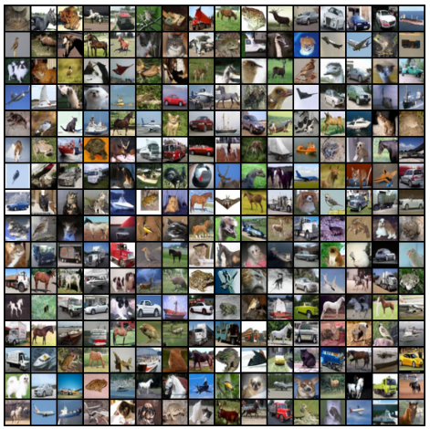
Figure 7: Generated CIFAR-10 samples without cherry-picking.

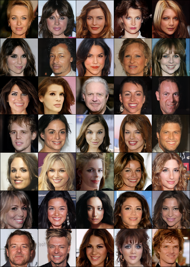
Figure 8: Generated CelebA-HQ-256 samples.

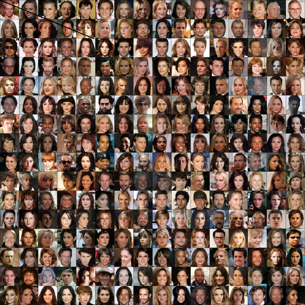
Figure 9: Generated CelebA-HQ-256 samples without cherry-picking.

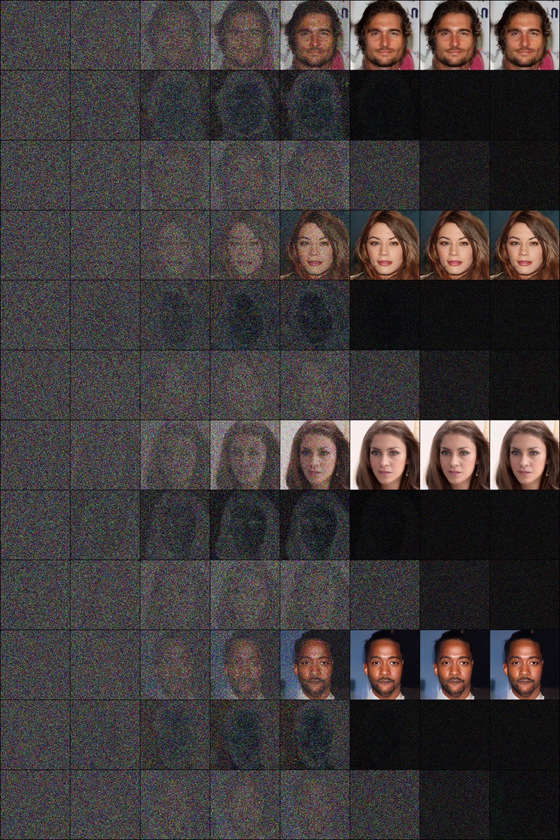
Figure 10: When sampling by integration of time-reverse HOLD’s ODE, CelebA-HQ-256 images, velocities, and accelerations are generated at different instants (as a percentage of total steps are 0., 0.5, 0.7, 0.8, 0.9, 0.99, 0.999, 0.99999) along the solution path.

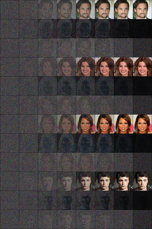
Figure 11: When sampling with LT sampler, CelebA-HQ-256 images, velocities, and accelerations are generated at different instants (as a percentage of total steps are 0., 0.5, 0.7, 0.8, 0.9, 0.93, 0.97, 0.99) along the solution path.

References

• [Anderson(1982)] B. D. Anderson. Reverse-time diffusion equation models. Stochastic Processes and their Applications, 12(3):313–326, 1982.
• [Baker(1901)] H. F. Baker. Further applications of metrix notation to integration problems. Proceedings of the London Mathematical Society, 1(1):347–360, 1901.
• [Bao et al.(2022)Bao, Li, Sun, Zhu, and Zhang] F. Bao, C. Li, J. Sun, J. Zhu, and B. Zhang. Estimating the optimal covariance with imperfect mean in diffusion probabilistic models. arXiv preprint arXiv:2206.07309, 2022.
• [Brock et al.(2019)Brock, Donahue, and Simonyan] A. Brock, J. Donahue, and K. Simonyan. Large scale GAN training for high fidelity natural image synthesis. In International Conference on Learning Representations, 2019. URL https://openreview.net/forum?id=B1xsqj09Fm.
• [Campbell(1896)] J. Campbell. On a law of combination of operators bearing on the theory of continuous transformation groups. Proceedings of the London Mathematical Society, 1(1):381–390, 1896.
• [Chen et al.(2018)Chen, Rubanova, Bettencourt, and Duvenaud] R. T. Chen, Y. Rubanova, J. Bettencourt, and D. K. Duvenaud. Neural ordinary differential equations. Advances in neural information processing systems, 31, 2018.
• [Chen et al.(2019)Chen, Behrmann, Duvenaud, and Jacobsen] R. T. Chen, J. Behrmann, D. K. Duvenaud, and J.-H. Jacobsen. Residual flows for invertible generative modeling. Advances in Neural Information Processing Systems, 32, 2019.
• [Dockhorn et al.(2021)Dockhorn, Vahdat, and Kreis] T. Dockhorn, A. Vahdat, and K. Kreis. Score-based generative modeling with critically-damped langevin diffusion. arXiv preprint arXiv:2112.07068, 2021.
• [Dockhorn et al.(2022)Dockhorn, Vahdat, and Kreis] T. Dockhorn, A. Vahdat, and K. Kreis. Genie: Higher-order denoising diffusion solvers. arXiv preprint arXiv:2210.05475, 2022.
• [Dormand and Prince(1980)] J. R. Dormand and P. J. Prince. A family of embedded runge-kutta formulae. Journal of computational and applied mathematics, 6(1):19–26, 1980.
• [Gao et al.(2020)Gao, Song, Poole, Wu, and Kingma] R. Gao, Y. Song, B. Poole, Y. N. Wu, and D. P. Kingma. Learning energy-based models by diffusion recovery likelihood. In International Conference on Learning Representations, 2020.
• [Goodfellow et al.(2014)Goodfellow, Pouget-Abadie, Mirza, Xu, Warde-Farley, Ozair, Courville, and Bengio] I. Goodfellow, J. Pouget-Abadie, M. Mirza, B. Xu, D. Warde-Farley, S. Ozair, A. Courville, and Y. Bengio. Generative adversarial nets. In Advances in Neural Information Processing Systems 27, volume 27, pages 2672–2680, 2014.
• [Grathwohl et al.(2018)Grathwohl, Chen, Bettencourt, Sutskever, and Duvenaud] W. Grathwohl, R. T. Chen, J. Bettencourt, I. Sutskever, and D. Duvenaud. Ffjord: Free-form continuous dynamics for scalable reversible generative models. arXiv preprint arXiv:1810.01367, 2018.
• [Hausdorff(1906)] F. Hausdorff. Die symbolische exponentialformel in der gruppentheorie. Ber. Verh. Kgl. SÃ chs. Ges. Wiss. Leipzig., Math.-phys. Kl., 58:19–48, 1906.
• [Heusel et al.(2017)Heusel, Ramsauer, Unterthiner, Nessler, and Hochreiter] M. Heusel, H. Ramsauer, T. Unterthiner, B. Nessler, and S. Hochreiter. Gans trained by a two time-scale update rule converge to a local nash equilibrium. Advances in neural information processing systems, 30, 2017.
• [Ho et al.(2020)Ho, Jain, and Abbeel] J. Ho, A. Jain, and P. Abbeel. Denoising diffusion probabilistic models. arXiv preprint arXiv:2006.11239, 2020.
• [Hyvärinen and Dayan(2005)] A. Hyvärinen and P. Dayan. Estimation of non-normalized statistical models by score matching. Journal of Machine Learning Research, 6(4), 2005.
• [Jolicoeur-Martineau et al.(2021)Jolicoeur-Martineau, Li, Piché-Taillefer, Kachman, and Mitliagkas] A. Jolicoeur-Martineau, K. Li, R. Piché-Taillefer, T. Kachman, and I. Mitliagkas. Gotta go fast with score-based generative models. In The Symbiosis of Deep Learning and Differential Equations, 2021.
• [Karras et al.(2018)Karras, Aila, Laine, and Lehtinen] T. Karras, T. Aila, S. Laine, and J. Lehtinen. Progressive growing of gans for improved quality, stability, and variation. In International Conference on Learning Representations, 2018.
• [Karras et al.(2020)Karras, Aittala, Hellsten, Laine, Lehtinen, and Aila] T. Karras, M. Aittala, J. Hellsten, S. Laine, J. Lehtinen, and T. Aila. Training generative adversarial networks with limited data. Advances in Neural Information Processing Systems, 33:12104–12114, 2020.
• [Karras et al.(2022)Karras, Aittala, Aila, and Laine] T. Karras, M. Aittala, T. Aila, and S. Laine. Elucidating the design space of diffusion-based generative models. In Advances in Neural Information Processing Systems, 2022.
• [Kim et al.(2021)Kim, Shin, Song, Kang, and Moon] D. Kim, S. Shin, K. Song, W. Kang, and I.-C. Moon. Score matching model for unbounded data score. arXiv preprint arXiv:2106.05527, 2021.
• [Kingma and Ba(2014)] D. P. Kingma and J. Ba. Adam: A method for stochastic optimization. arXiv preprint arXiv:1412.6980, 2014.
• [Kingma and Dhariwal(2018)] D. P. Kingma and P. Dhariwal. Glow: Generative flow with invertible 1x1 convolutions. Advances in neural information processing systems, 31, 2018.
• [Kingma and Welling(2014)] D. P. Kingma and M. Welling. Auto-encoding variational bayes. In ICLR 2014 : International Conference on Learning Representations (ICLR) 2014, 2014.
• [Kong and Ping(2021)] Z. Kong and W. Ping. On fast sampling of diffusion probabilistic models. arXiv preprint arXiv:2106.00132, 2021.
• [Leimkuhler and Matthews(2015)] B. Leimkuhler and C. Matthews. Molecular Dynamics: With Deterministic and Stochastic Numerical Methods, volume 39. Springer, 2015.
• [Li et al.(2022)Li, Thickstun, Gulrajani, Liang, and Hashimoto] X. L. Li, J. Thickstun, I. Gulrajani, P. Liang, and T. B. Hashimoto. Diffusion-lm improves controllable text generation. arXiv preprint arXiv:2205.14217, 2022.
• [Liu et al.(2022)Liu, Ren, Lin, and Zhao] L. Liu, Y. Ren, Z. Lin, and Z. Zhao. Pseudo numerical methods for diffusion models on manifolds. arXiv preprint arXiv:2202.09778, 2022.
• [Lu et al.(2022)Lu, Zhou, Bao, Chen, Li, and Zhu] C. Lu, Y. Zhou, F. Bao, J. Chen, C. Li, and J. Zhu. Dpm-solver: A fast ode solver for diffusion probabilistic model sampling in around 10 steps. arXiv preprint arXiv:2206.00927, 2022.
• [Meng et al.(2021)Meng, Song, Song, Wu, Zhu, and Ermon] C. Meng, Y. Song, J. Song, J. Wu, J.-Y. Zhu, and S. Ermon. Sdedit: Image synthesis and editing with stochastic differential equations. arXiv preprint arXiv:2108.01073, 2021.
• [Mou et al.(2021)Mou, Ma, Wainwright, Bartlett, and Jordan] W. Mou, Y.-A. Ma, M. J. Wainwright, P. L. Bartlett, and M. I. Jordan. High-order langevin diffusion yields an accelerated mcmc algorithm. J. Mach. Learn. Res., 22:42–1, 2021.
• [Neal(2011)] R. M. Neal. Mcmc using hamiltonian dynamics. Handbook of markov chain monte carlo, 2(11):2, 2011.
• [Nichol and Dhariwal(2021)] A. Q. Nichol and P. Dhariwal. Improved denoising diffusion probabilistic models. In International Conference on Machine Learning, pages 8162–8171. PMLR, 2021.
• [Parmar et al.(2021)Parmar, Li, Lee, and Tu] G. Parmar, D. Li, K. Lee, and Z. Tu. Dual contradistinctive generative autoencoder. In Proceedings of the IEEE/CVF Conference on Computer Vision and Pattern Recognition, pages 823–832, 2021.
• [Popov et al.(2021)Popov, Vovk, Gogoryan, Sadekova, Kudinov, and Wei] V. Popov, I. Vovk, V. Gogoryan, T. Sadekova, M. Kudinov, and J. Wei. Diffusion-based voice conversion with fast maximum likelihood sampling scheme. arXiv preprint arXiv:2109.13821, 2021.
• [Putzer(1966)] E. J. Putzer. Avoiding the jordan canonical form in the discussion of linear systems with constant coefficients. The American Mathematical Monthly, 73(1):2–7, 1966.
• [Rombach et al.(2022)Rombach, Blattmann, Lorenz, Esser, and Ommer] R. Rombach, A. Blattmann, D. Lorenz, P. Esser, and B. Ommer. High-resolution image synthesis with latent diffusion models. In Proceedings of the IEEE/CVF Conference on Computer Vision and Pattern Recognition, pages 10684–10695, 2022.
• [Särkkä and Solin(2019)] S. Särkkä and A. Solin. Applied stochastic differential equations, volume 10. Cambridge University Press, 2019.
• [Shi and Wu(2022)] Z. Shi and S. Wu. Itôn: End-to-end audio generation with itô stochastic differential equations. Digital Signal Processing, page 103781, 2022.
• [Sohl-Dickstein et al.(2015)Sohl-Dickstein, Weiss, Maheswaranathan, and Ganguli] J. Sohl-Dickstein, E. Weiss, N. Maheswaranathan, and S. Ganguli. Deep unsupervised learning using nonequilibrium thermodynamics. In International Conference on Machine Learning, pages 2256–2265. PMLR, 2015.
• [Song et al.(2020a)Song, Meng, and Ermon] J. Song, C. Meng, and S. Ermon. Denoising diffusion implicit models. In International Conference on Learning Representations, 2020a.
• [Song and Ermon(2019)] Y. Song and S. Ermon. Generative modeling by estimating gradients of the data distribution. arXiv preprint arXiv:1907.05600, 2019.
• [Song and Ermon(2020)] Y. Song and S. Ermon. Improved techniques for training score-based generative models. Advances in neural information processing systems, 33:12438–12448, 2020.
• [Song et al.(2020b)Song, Sohl-Dickstein, Kingma, Kumar, Ermon, and Poole] Y. Song, J. Sohl-Dickstein, D. P. Kingma, A. Kumar, S. Ermon, and B. Poole. Score-based generative modeling through stochastic differential equations. arXiv preprint arXiv:2011.13456, 2020b.
• [Song et al.(2021)Song, Durkan, Murray, and Ermon] Y. Song, C. Durkan, I. Murray, and S. Ermon. Maximum likelihood training of score-based diffusion models. Advances in Neural Information Processing Systems, 34:1415–1428, 2021.
• [Strang(1968)] G. Strang. On the construction and comparison of difference schemes. SIAM journal on numerical analysis, 5(3):506–517, 1968.
• [Trotter(1959)] H. F. Trotter. On the product of semi-groups of operators. Proceedings of the American Mathematical Society, 10(4):545–551, 1959.
• [Tuckerman(2010)] M. Tuckerman. Statistical mechanics: theory and molecular simulation. Oxford university press, 2010.
• [Vahdat et al.(2021)Vahdat, Kreis, and Kautz] A. Vahdat, K. Kreis, and J. Kautz. Score-based generative modeling in latent space. Advances in Neural Information Processing Systems, 34:11287–11302, 2021.
• [Vincent(2011)] P. Vincent. A connection between score matching and denoising autoencoders. Neural computation, 23(7):1661–1674, 2011.
• [Wang et al.(2021)Wang, Jiao, Xu, Wang, and Yang] G. Wang, Y. Jiao, Q. Xu, Y. Wang, and C. Yang. Deep generative learning via schrödinger bridge. In International Conference on Machine Learning, pages 10794–10804. PMLR, 2021.
• [Watson et al.(2021)Watson, Ho, Norouzi, and Chan] D. Watson, J. Ho, M. Norouzi, and W. Chan. Learning to efficiently sample from diffusion probabilistic models. arXiv preprint arXiv:2106.03802, 2021.
• [Xiao et al.(2020)Xiao, Kreis, Kautz, and Vahdat] Z. Xiao, K. Kreis, J. Kautz, and A. Vahdat. Vaebm: A symbiosis between variational autoencoders and energy-based models. In International Conference on Learning Representations, 2020.
• [Xu et al.(2023)Xu, Liu, Tian, Tong, Tegmark, and Jaakkola] Y. Xu, Z. Liu, Y. Tian, S. Tong, M. Tegmark, and T. Jaakkola. Pfgm++: Unlocking the potential of physics-inspired generative models. arXiv preprint arXiv:2302.04265, 2023.
• [Zhang and Chen(2022)] Q. Zhang and Y. Chen. Fast sampling of diffusion models with exponential integrator. arXiv preprint arXiv:2204.13902, 2022.