Black Hole shadows of $\alpha^{\prime}$-corrected black holes

Abstract

In this paper we study the qualitative features induces by corrections to GR coming from String Theory, on the shadows of rotating black holes. We deal with the slowly rotating black hole solutions up to order $\mathcal{O}(a^{3})$, to first order in $\alpha^{\prime}$, including also the dilaton. We provide a detailed characterization of the geometry, as well as the ISCO and photon ring, and then we proceed to obtain the black hole images within the relativistic thin-disk model. We characterize the images by computing the diameter, displacement and asymmetry. A comparison with the Kerr case, indicates that all these quantities grow due to the $\alpha^{\prime}$ correction, and that the departure from GR for different observable is enhanced depending on the angle of view, namely for the diameter the maximum departure is obtained when the system is face-on, while for the displacement and asymmetry the departure from GR is maximized for edge-on point of view.

I Introduction

Over the last decades, the detection of compact objects such as black holes has increased significantly, especially with new generations of instrumentation for the observation and detection of black holes. These go from interferometers that detect gravitational waves from black hole binaries such as the LIGO-VIRGO collaboration [1], to the direct observation of these objects with the Event Horizon Telescope (EHT). The latter has obtained the first images of supermassive black holes (SMBH) at the center of the M87 galaxy [2], as well as at the center of our own galaxy with the image of the Sgr A* SMBH [3]. These results define historical and crucial achievements in testing the theory of General Relativity (GR) and serve as laboratories for testing it in the strong field regime. More recent results include the study of the relativistic jets of these systems, as well as the observation of polarization emission due to the magnetized environment [4, 5, 6].

While GR has been able to describe the current observations to a high precision, it is well-known that there are both theoretical and experimental reasons that indicate the need of an extension of such framework, including the failure to predict the accelerating expansion of the Universe, to incorporate dark matter, as well as the incompatibility with quantum field theory.

In this context, the inclusion of direct observation of SMBHs creates a great opportunity to test and constrain the effects of modified gravity theories in environments close them, which will even further improve with future facilities like the ngEHT (Next Generation Event Horizon Telescope) project, which aims at increasing the baseline by incorporating satellites, thereby improving on the resolution within the images, allowing for instance for very precise measurements of the black hole spin [8].

It is currently accepted that GR has to be interpreted as an effective field theory (EFT), emerging from a UV-complete framework, in the low energy limit. Within such setup, corrections to GR are expected, which come suppressed by a perturbative parameter. In the context of String Theory, such corrections come multiplied by $\alpha^{\prime}$, namely by one over the string tension, and are in general hard to compute. Even more, since String Theory is consistently formulated in dimension ten, a compactification scheme is necessary to connect the theory with four-dimensional physics. Generically, the four-dimensional Einstein-Hilbert term, is supplemented by higher dimensional operators, which perturbativelly modify the dynamics and the structure of the solutions.

The aim of this work is to establish the qualitative features that such terms may imprint on the shadows of rotating black holes.

It is important to mention that the order of magnitude of $\alpha^{\prime}$ is expected to be much lower than the values here considered, notwithstanding this paper is devoted to study in a qualitative manner the signals induced by the $\alpha^{\prime}$-corrections on the black hole images. This paper is organized as follows: Section II introduces the theory containing both the metric and the dilaton field, on the string frame, together with the correction up to first order in $\alpha^{\prime}$. It also contains the field equations that a perturbative solution may fulfill, by expanding around a constant dilaton background and an Einstein geometry. Section III reviews the construction of the $\alpha^{\prime}$-corrected, slowly rotating black hole up to $\mathcal{O}(a^{3},a^{2}\alpha,\alpha^{2})$, presenting the expressions for the temperature, entropy, angular velocity of the horizon and the first law of black hole thermodynamics. Section IV contains the computation of the Petrov type, the location of the event horizon and ergosphere, and an upper bound on $\alpha$ that ensures the spacetime interpretation of the perturbative, rotating solution. It also provides a detailed characterization of the geodesics with particular emphasis on the expression for the Innermost Stable Circular Orbits (ISCO) and the photon ring, that are of uttermost importance for the computation of the shadows. Section V, introduces the numerical model where the emission of the relativistic accretion disk is treated along the thin-disk, Novikov-Thorne model. The section also contains a review of the Ray-tracing code. Section VI presents the results of the simulations for the black hole shadows, for different values of $\alpha^{\prime}$, focusing on the signals induced on the diameter, displacement and asymmetry of the images, induced by the stringy corrections. Section VII contains conclusion and further comments.

II The theory

The theory we will consider emerges from the low-energy effective action of String Theory including $\alpha^{\prime}$ corrections to the dilaton-graviton sector. Neglecting order $\mathcal{O}(\alpha^{\prime 2})$ terms, we are able to perform a suitable field redefinition such that the field equations are of second order for both the metric and the dilaton, leading to the action principle [9], [10] (see also [11] and [12])

$$I[g_{\mu\nu},\phi] =\int\mathrm{d}^{4}x\sqrt{-g}e^{-2\phi}[R+4(\partial\phi)^{2}$$

$$+\alpha(\mathcal{X}_{4}-16(\partial_{\mu}\phi\partial^{\mu}\phi)^{2}+\mathcal{O}(\alpha^{2})]\ ,$$ (1)

where the Euler density is defined as

$$\mathcal{X}_{4} =R_{\mu\nu\rho\sigma}R^{\mu\nu\rho\sigma}-4R_{\mu\nu}R^{\mu\nu}+R^{2}$$ (2)

providing second order equations in an explicit manner. Here the constant $\alpha=\alpha^{\prime}/8$. See [13] for the precise dimensional reduction and consistent truncation of String Theory leading to the action principle (1) and [12] for the field redefinition that allows connecting both scenarios. The field equations derived from (1) are

$$R_{\mu\nu}+2\phi_{;\nu;\mu}+\alpha\mathcal{H}_{\mu\nu} =0\,,$$ (3)

$$R-4(\partial\phi)^{2}+\alpha\mathcal{P} =0\,,$$ (4)

where semi-colon denotes covariant derivative and

$$\mathcal{H}_{\mu\nu} =-4\phi_{;\nu;\mu}(\partial\phi)^{2}+8\phi^{;\sigma}{}_{;\mu}\phi_{;\nu;\sigma}$$ (5)

$$-16\phi_{(;\mu}\phi_{;\nu);\sigma}\phi^{;\sigma}+2(\phi^{;\sigma;\lambda}-2\phi^{;\sigma}\phi^{;\lambda})R_{\mu\sigma\lambda\nu}$$

$$+g_{\mu\nu}[-56(\partial\phi)^{4}-12\phi_{;\lambda;\sigma}\phi^{;\lambda;\sigma}$$

$$-24\phi_{;\rho;\sigma}\phi^{;\rho}\phi^{;\sigma}+\frac{1}{2}R_{\lambda\delta\rho\sigma}R^{\lambda\delta\rho\sigma}]\,,$$

$$\mathcal{P} =R_{\lambda\delta\rho\sigma}R^{\lambda\delta\rho\sigma}-16\phi_{;\mu;\nu}\phi^{;\mu;\nu}+$$ (6)

$$-64\phi^{;\rho;\sigma}\phi_{;\rho}\phi_{;\sigma}-96(\partial\phi)^{4}\,.$$

Provided the fact that the action (1) is consistent neglecting $\mathcal{O}(\alpha^{2})$, we are interested in studying consistent $\alpha^{\prime}$–corrections of configurations $\overline{g}_{\mu\nu}$ and $\overline{\phi}$ satisfying the equations (3) and (4) with $\alpha=0$. Therefore, the general correction should be of the form

$$g_{\mu\nu} =\overline{g}_{\mu\nu}+\alpha\gamma_{\mu\nu}+\mathcal{O}(\alpha^{2})\,,$$ (7)

$$\phi =\overline{\phi}+\alpha\tau+\mathcal{O}(\alpha^{2})\,.$$ (8)

where $\gamma_{\mu\nu}$ is a symmetric perturbative tensor and $\tau$ is a scalar function of the spacetime coordinates. The situation in which $\overline{\phi}=\phi_{0}$ is a constant is particularly interesting since the equations for $\overline{g}_{\mu\nu}$ consistently reduce to the vacuum Einstein equations, and we will focus in such case through out this work. It is interesting to notice that due to the fact that the dilaton appears linearly in the equation (3), then a consistent correction at order $\alpha$ to the metric is allowed. Consider the leading term of the dilaton being a constant and the leading term of the metric a solution of the vacuum Einstein equations, then a huge simplification of the equations (3) and (4) takes place leading to

$$\alpha\Pi_{\mu\nu}+2\alpha\overline{\nabla}_{\mu}\partial_{\nu}\tau+\frac{1}{2}\alpha\overline{g}_{\mu\nu}\overline{\mathcal{K}} =0\,,$$ (9)

$$\alpha\overline{\Pi}_{\mu}{}^{\mu}+4\alpha\overline{\nabla}^{\mu}\partial_{\mu}\tau+\alpha\overline{\mathcal{K}} =0\,.$$ (10)

where

$$\Pi_{\mu\nu} =\overline{\nabla}^{\lambda}\overline{\nabla}_{(\mu}\gamma_{\nu)\lambda}-\frac{1}{2}\overline{\nabla}^{\lambda}\overline{\nabla}_{\lambda}\gamma_{\mu\nu}-\frac{1}{2}\overline{\nabla}_{\mu}\partial_{\nu}\gamma_{\lambda}{}^{\lambda}\,,$$

$$\overline{\mathcal{K}} =R_{\lambda\delta\rho\sigma}R^{\lambda\delta\rho\sigma}|_{\overline{g}_{\mu\nu}}\,.$$

The barred covariant derivatives are computed with the Levi-Civita connection associated to the metric $\overline{g}_{\mu\nu}$. This equation can be integrated in a variety of situations as was shown in [12] for accelerating black holes and slowly rotating black holes. We will analyze in detail the later situation in which the seed metric is the Kerr spacetime expanded up to second order on the rotation parameter $a=GJ/M$.

III Slowly rotating $\alpha^{\prime}-$ corrected BH

The slowly rotating black hole solution found in [12] corresponds to a consistent solution of the equations (9) and (10) for $\overline{g}_{\mu\nu}$ being the slowly rotating Kerr metric with rotation parameter $a$, expanded up to $a^{2}$ neglecting terms $\mathcal{O}(a^{3})$. We find that it is possible to integrate the equation even considering the logarithmic branch, controlled by an integration constant $b$, in the $\alpha$-corrected static configuration. An analytic solution of (9)-(10) at non-linear level in the rotation parameter is still not known in the literature, nevertheless higher order correction in $a$ could be obtained along the lines of [13]. The slowly rotating spacetime, neglecting orders $\mathcal{O}(a^{2}\alpha,a^{3},\alpha^{2})$, including the logarithmic branch is given by

$$g_{tt} =-1+\frac{2M}{r}+\frac{2Ma^{2}\cos^{2}\theta}{r^{3}}-\alpha f_{1}(r)\,,$$ (11)

$$g_{t\phi} =-\frac{2Ma\sin^{2}\theta}{r}+a\alpha h_{1}(r,\theta)\,,$$ (12)

$$g_{rr} =\frac{1}{1-\frac{2M}{r}+\alpha g_{1}(r)}-a^{2}\frac{(2M-r)\cos^{2}\theta+r}{(2M-r)^{2}r}\,,$$ (13)

$$g_{\theta\theta} =r^{2}+a^{2}\cos\theta\,,$$ (14)

$$g_{\phi\phi} =(r^{2}+a^{2}+\frac{2Ma^{2}\sin^{2}\theta}{r})\sin^{2}\theta\,,$$ (15)

where

$$f_{1}(r) =\frac{8M^{2}}{r^{4}}+\frac{10M}{3r^{3}}+\frac{4}{r^{2}}-\frac{4}{Mr}-\frac{4bM}{r}+$$ (16)

$$+\frac{b(r-3M)}{r}\log\left[\left(1-\frac{2M}{r}\right)^{2}\right]$$

$$g_{1}(r) =-\frac{40M^{2}}{3r^{4}}+\frac{2M}{r^{3}}+\frac{2}{r^{2}}+$$ (17)

$$-\frac{bM}{r}\log\left[\left(1-\frac{2M}{r}\right)^{2}\right]\,,$$

$$h_{1}(r,\theta) =\left(\frac{8M^{2}}{r^{4}}+\frac{6M}{r^{3}}+\frac{6}{r^{2}}+\right.$$ (18)

$$\left.-\frac{3bM}{r}\log\left[\left(1-\frac{2M}{r}\right)^{2}\right]\right)\sin^{2}\theta\,.$$ (19)

While the dilaton field is given by

$$\phi =\phi_{0}+\alpha\left(-\frac{4M}{3r^{3}}-\frac{1}{r^{2}}-\frac{1}{Mr}+\frac{b}{2}\log\left[\left(1-\frac{2M}{r}\right)^{2}\right]\right)$$

In spite of the generalization including the logarithmic branch to the slowly rotating solution, we will concentrate through out this article in the $b=0$ case. Using the Iyer-Wald method to compute conserved charges for the theory (1) as was explained in [12] the mass and the angular momentum neglecting $\mathcal{O}(a^{3},a^{2}\alpha)$ are respectively

$$\mathcal{M} =\frac{M}{G}+\frac{\alpha}{GM}\,,$$ (20)

$$\mathcal{J} =\frac{aM}{G}\,.$$ (21)

The deviation tensor $\gamma_{\mu\nu}$ is present in the components $g_{tt},g_{t\phi}$ and $g_{rr}$. Note also that the $\gamma_{\mu\nu}$ goes to zero fast enough as $r\to\infty$ thus the spacetime is asymptotically flat, and the Iyer-Wald charges converge. The Hawking temperature and entropy, computed from the Wald formula [14], of the slowly rotating black hole (11) with $b=0$ do not receive an $a\alpha$ correction and are given by

$$T =\frac{1}{8\pi M}-\frac{\alpha}{8\pi M^{3}}-\frac{a^{2}}{32\pi M^{3}}\,,$$ (22)

$$\mathcal{S} =\frac{4M^{2}\pi}{G}+\frac{12\pi\alpha}{G}-\frac{\pi a^{2}}{G}\,,$$ (23)

where consistently with the scenario we are dealing with, we have neglected terms $\mathcal{O}(a^{3},a^{2}\alpha)$. The angular velocity of the horizon of the slowly rotating black hole is

$$\Omega_{\mathrm{bh}} =\frac{a}{4M^{2}}-\frac{3a\alpha}{4M^{4}}+\mathcal{O}(a^{3},a\alpha)\,.$$ (24)

The first law of thermodynamics holds by considering the variation with respect to the integration constants $M$ and $a$ and considering the variation of the perturbative parameter $\delta a$ being of order $a$

$$\delta\mathcal{M} =T\delta\mathcal{S}+\Omega_{\mathrm{bh}}\delta\mathcal{J}\,,$$ (25)

again neglecting $\mathcal{O}(a^{3},a^{2}\alpha,\alpha^{2})$.

IV Spacetime properties

In this section we will describe further properties of the slowly rotating $\alpha^{\prime}$-corrected geometry, comparing them with the Kerr slowly rotating case. These properties will be important for the simulations of the black hole shadows.

IV.1 Petrov clasification

To determine the Petrov type of the slowly rotating spacetime we compute the Weyl tensor in null tetrad basis. For that, we define the following orthonormal basis in terms of the metric component (11)

$$e^{0} =\sqrt{-g_{tt}}\mathrm{d}t-\frac{g_{t\phi}}{\sqrt{-g_{tt}}}\mathrm{d}\phi\,,$$ (26)

$$e^{1} =\sqrt{g_{rr}}\mathrm{d}r\,,\quad e^{2}=\sqrt{g_{\theta\theta}}\mathrm{d}\theta\,,$$

$$e^{3} =\sqrt{g_{\phi\phi}-\frac{g_{t\phi}^{2}}{g_{tt}}}\mathrm{d}\phi\,,$$

which must be expanded in $a$ and $\alpha$ neglecting $\mathcal{O}(a^{3},\alpha^{2},a^{2}\alpha)$. In such frame the null tetrad is defined by

$$k_{\mu} =\frac{1}{\sqrt{2}}(e^{0}{}_{\mu}+e^{3}{}_{\mu})\,,\,l_{\mu}=\frac{1}{\sqrt{2}}(e^{0}{}_{\mu}-e^{3}{}_{\mu})\,,$$ (27)

$$m_{\mu} =\frac{1}{\sqrt{2}}(e^{1}{}_{\mu}-ie^{2}{}_{\mu})\,,\,\overline{m}_{\mu}=\frac{1}{\sqrt{2}}(e^{1}{}_{\mu}+ie^{2}{}_{\mu})\,.$$

The components of the Weyl tensor in the null basis are given by the projections

$$\Psi_{0}=C_{\mu\nu\rho\sigma}k^{\mu}m^{\nu}k^{\rho}m^{\sigma}\,,\,\Psi_{1}=C_{\mu\nu\rho\sigma}k^{\mu}l^{\nu}k^{\rho}m^{\sigma}\,,$$

$$\Psi_{2}=C_{\mu\nu\rho\sigma}k^{\mu}m^{\nu}\overline{m}^{\rho}l^{\sigma}\,,\,\Psi_{3}=C_{\mu\nu\rho\sigma}l^{\mu}k^{\nu}l^{\rho}\overline{m}^{\sigma}\,,$$

$$\Psi_{4}=C_{\mu\nu\rho\sigma}l^{\mu}\overline{m}^{\nu}l^{\rho}\overline{m}^{\sigma}\,.$$ (28)

For the spacetime (11) the following expressions hold

$$\Psi_{0} =\mathcal{O}(a^{3},\alpha^{2},a^{2}\alpha)\,,$$

$$\Psi_{3} =\mathcal{O}(a^{3},\alpha^{2},a^{2}\alpha)\,,$$

$$\Psi_{0}\Psi_{4}-9(\Psi_{2})^{2} =\mathcal{O}(a^{3},\alpha^{2},a^{2}\alpha)\,.$$

Indicating that the corrected spacetime is Petrov type D, as the seed spacetime.

IV.2 Event horizon and ergosphere

In [12] the location of the event horizon for a non-rotating black hole was calculated from the conditions $g^{rr}(r_{+})=g_{tt}(r_{+})=0$, assuming that $r_{+}=2M+\alpha\mu_{1}$. Solving for $\mu_{1}$, the location of the horizon was found at

$$r_{+}=2M+\dfrac{\alpha}{6M}.$$ (29)

Furthermore, the rotating case possesses a curvature singularity at $r=0$, this can be inferred by analyzing the Kretschmann scalar

$$R_{\mu\nu\rho\sigma}R^{\mu\nu\rho\sigma} = \frac{48M^{2}}{r^{6}}-\frac{1008\cos^{2}\theta M^{2}a^{2}}{r^{8}}$$

$$+ \frac{\left(-128M^{3}-96M^{2}r-96M\,r^{2}+96r^{3}\right)\alpha}{r^{9}},$$

which diverges as $r\rightarrow 0$. The rotating spacetime also possesses an event horizon, located at $r=r_{+}$ such that $g^{rr}\left(r_{+}\right)=0$ , which turns out to be equivalent to the condition

$$g_{tt}g_{\phi\phi}-g_{t\phi}^{2}=0,$$ (31)

Solving this equation using the location of the horizon in the Kerr metric and with the ansatz $r_{+}^{\alpha^{\prime}}=r_{+}^{SK}+\alpha\mu_{1}$, we found that the location of the event horizon for this spacetime is

$$r_{+}=2M-\frac{a^{2}}{2M}+\frac{\alpha}{6M}+\mathcal{O}(a^{2}\alpha,\alpha^{2}).$$ (32)

Using the condition $g_{tt}(r)=0$ to find the location of the ergosphere, one finds

$$r_{erg}^{\alpha^{\prime}}=2M-\frac{a^{2}}{2M}\cos^{2}\theta-\dfrac{\alpha}{12M^{2}}+\mathcal{O}(a^{2}\alpha,\alpha^{2}).$$ (33)

Note that the $\alpha^{\prime}$-corrected ergosphere is smaller than the ergosphere of Kerr, namely $r^{\alpha^{\prime}}_{\mathrm{erg}}<r_{\mathrm{erg}}^{SK}$, while the location of the event horizon of the $\alpha^{\prime}$-corrected geometry is larger than the location of the Kerr event horizon.

IV.3 Lorentz signature

We will be exploring the geodesic orbits on this geometry, therefore, we impose the preservation of the Lorentzian signature as a consistency constraint on the perturbative construction. Since, the determinant of the Slowly rotating Kerr metric is given by

$$g^{SK}=-r^{2}\sin^{2}\theta\left(2a^{2}\cos^{2}\theta+r^{2}\right)\ ,$$ (34)

the determinant of the spacetime defined by the metric functions (11) is

$$g^{\alpha^{\prime}}=g^{SK}+\frac{\alpha\left(32M^{2}r+18Mr^{2}+12r^{3}\right)\sin^{2}\theta}{3M}.$$ (35)

As we remark, the $\alpha^{\prime}$-correction in the metric tensor goes to zero at spatial infinity, thus the signature of the metric can change only in the interior of the spacetime. In particular we are interested in the signature of the metric in the near horizon region. Computing the quotient between the slowly rotating Kerr determinant and the corrected metric determinant we can find some restrictions for the possible values of the $\alpha^{\prime}$ parameter

$$\frac{g^{\alpha^{\prime}}}{g^{SK}}=1-\alpha\left(\frac{32M}{3r^{3}}+\frac{6}{r^{2}}+\frac{4}{Mr}\right)\,.$$ (36)

To preserve the signature of the spacetime outside the horizon, namely $r\geq r_{+}$, it is a necessary condition that the second term of (36) to be smaller than 1. In particular, close to the horizon $r=r_{+}^{\alpha^{\prime}}$, the signature should be preserved as well

$$\frac{g^{\alpha^{\prime}}}{g^{SK}}(r_{+})=1-\frac{29\alpha}{6M^{2}}+\mathcal{O}(a^{2}\alpha,\alpha^{2}),$$ (37)

where we have expanded around the rotation parameter and the coupling term. This equation leads to the bound

$$\alpha<\frac{6M^{2}}{29}+\mathcal{O}(a^{2}\alpha,\alpha^{2}),$$ (38)

which is a consistent upper limit for the $\alpha$ coupling.

IV.4 Circular geodesic motion

The circular geodesic motion around compact objects for a stationary axisymmetric space-time can be described with the equatorial approximation, $|\theta-\frac{\pi}{2}|\ll 1$. Therefore, under this condition, the components of the metric $g_{\mu\nu}$ depends only on the radial coordinate $r$. The geodesic equation reads

$$\frac{d^{2}x^{\alpha}}{d\tau^{2}}=-\Gamma^{\alpha}_{\beta}{}_{\gamma}\frac{dx^{\beta}}{d\tau}\frac{dx^{\gamma}}{d\tau},$$ (39)

where $\Gamma^{\alpha}_{\beta}{}_{\gamma}$ are the Christoffel symbols and $\tau$ is the affine parameter. Since the metric presents axi- and reflection symmetry, for particles on circular orbits, the geodesic equation in the radial direction, $\alpha=r$ in (39), reduces to

$$\frac{1}{2}\partial_{r}g_{tt}\left(\frac{dt}{d\tau}\right)^{2}+\partial_{r}g_{t\phi}\frac{dt}{d\tau}\frac{d\phi}{d\tau}+\frac{1}{2}\partial_{r}g_{\phi\phi}\left(\frac{d\phi}{d\tau}\right)^{2}=0,$$ (40)

where $\partial_{r}=\partial/\partial r$. From this equation, the Keplerian frequency in the equatorial plane can be expressed as

$$\Omega_{\phi} = \frac{p^{\phi}}{p^{t}}=\frac{-\partial_{r}g_{t\phi}\pm\sqrt{(\partial_{r}g_{t\phi})^{2}-\partial_{r}g_{tt}\partial_{r}g_{\phi\phi}}}{\partial_{r}g_{\phi\phi}},$$ (41)

$$p^{\phi} \equiv \dot{\phi}\,,\quad p^{t}\equiv\dot{t}\,,$$ (42)

where the upper sign refers to prograde orbits and the lower sign to retrograde orbits, depending on the value of the spin parameter $a$.

Since the metric $g_{\mu\nu}$ is stationary and axisymmetric (i.e independent of the $t$ and $\phi$ coordinates), it has a timelike and an azimuthal Killing vector, leading to the existence of two conseved quantities, the specific energy $\tilde{E}$ and the specific angular momentum $\tilde{L}$. Those correspond to the $p_{t}=-\tilde{E}$ and $p_{\phi}=\tilde{L}$ components of the four-momentum, from which the following geodesic equations can be derived,

$$\dot{t}=\frac{\tilde{E}g_{\phi\phi}+\tilde{L}g_{t\phi}}{g_{t\phi}^{2}-g_{tt}g_{\phi\phi}},\\$$ (43)

$$\dot{\phi}=-\frac{\tilde{E}g_{t\phi}+\tilde{L}g_{tt}}{g_{t\phi}^{2}-g_{tt}g_{\phi\phi}},$$ (44)

where $\dot{t}=dt/d\tau$ and $\dot{\phi}=d\phi/d\tau$.

The four momentum is normalized as

$$g_{\mu\nu}p^{\mu}p^{\nu}=p^{\mu}p_{\mu}=-\epsilon^{2},$$ (45)

where $\epsilon^{2}=+1,-1,$ for time-like and space-like geodesics, respectively. As usual, it is possible to obtain the expression for the effective potential in the equatorial plane as follows

$$g_{rr}\dot{r}^{2}=V_{eff}(r)\ ,$$ (46)

where the effective potential is given by

$$V_{eff}(r)=-\epsilon^{2}+\frac{\tilde{E}^{2}g_{\phi\phi}+2\tilde{E}\tilde{L}g_{t\phi}+\tilde{L}^{2}g_{tt}}{g_{t\phi}^{2}-g_{tt}g_{\phi\phi}}\ .$$ (47)

Our primary focus is on circular orbits confined to the equatorial plane for massive, timelike particles ($\epsilon^{2}=1$), for which the orbits are governed by

$$V_{eff}(r)=0,$$ (48)

$$\frac{\partial}{\partial r}V_{eff}(r)=0.$$ (49)

Using these conditions it is possible to obtain the expression for the specific energy $\tilde{E}$ and angular momentum $\tilde{L}$ in a circular orbit

$$\tilde{E}=\frac{-g_{tt}-g_{t\phi}\Omega_{\phi}}{\sqrt{-g_{tt}-2g_{t\phi}\Omega-g_{\phi\phi}\Omega^{2}}},$$ (50)

$$\tilde{L}=\frac{g_{t\phi}+g_{\phi\phi}\Omega_{\phi}}{\sqrt{-g_{tt}-2g_{t\phi}\Omega-g_{\phi\phi}\Omega^{2}}}.$$ (51)

On the other hand, since one of our goals is to obtain simulations of a thin accretion disk around a black hole described by this solution, we must determine the location of ISCO. It is possible to find it from the condition $\partial^{2}V_{eff}(r)/\partial r^{2}=0$, which leaves us with the following expression

$$\tilde{E}^{2}\partial_{r}^{2}g_{\phi\phi}+2\tilde{E}\tilde{L}\partial_{r}^{2}g_{t\phi}+\tilde{L}^{2}\partial_{r}^{2}g_{tt}-\partial_{r}^{2}(g_{t\phi}^{2}-g_{tt}g_{\phi\phi})=0.$$ (52)

Since the metric given by Eq. (11) satisfies all the characteristics previously mentioned, it is possible to obtain the Keplerian frequency from Eq. (53) in $\mathcal{O}(\alpha)$, leading to

$$\Omega_{\phi} = -\frac{Ma}{r^{3}}\pm\sqrt{\frac{M}{r}}\frac{\left(M^{3}a^{2}+M^{2}r^{3}\right)}{r^{4}M^{2}}$$ (53)

$$\pm \frac{\alpha\left(-8M^{3}-\frac{5}{2}r\,M^{2}-2M\,r^{2}+r^{3}\right)}{r^{\frac{9}{2}}M^{\frac{3}{2}}}$$

$$+ \frac{a\alpha\left(32M^{2}+18Mr+12r^{2}\right)}{2r^{6}}\ .$$

The expressions for the specific energy and angular momentum, from Eqs. (50-51) at $\mathcal{O}(\alpha)$ are

$$\tilde{E}= \frac{r-2M}{r^{1/2}(r-3M)^{1/2}}+\frac{a^{2}M^{2}}{2\sqrt{r}(r-3M)^{5/2}}$$ (54)

$$\mp\frac{aM^{3/2}}{r(r-3M)^{3/2}}$$

$$-\alpha\frac{(34M^{3}+29M^{2}r-36Mr^{2}+6r^{3})}{6Mr^{5/2}(r-3M)^{3/2}}$$

$$\mp\frac{\alpha a}{6\sqrt{M}r^{4}(r-3M)^{5/2}}(120M^{4}-16M^{3}r+$$

$$+15M^{2}r^{2}-12Mr^{3}+6r^{4})$$

and

$$\tilde{L}= \pm\frac{rM^{1/2}}{(r-3M)^{1/2}}-a\frac{3M(r-2M)}{\sqrt{r}(r-3M)^{3/2}}+$$ (55)

$$\pm\frac{a^{2}M^{1/2}}{2r(r-3M)^{5/2}}(6M^{2}-5Mr+2r^{2})+$$

$$+\frac{\alpha a}{2r^{5/2}(r-3M)^{5/2}}(18M^{3}+25M^{2}r$$

$$-6Mr^{2}-6r^{3})+$$

$$\pm\frac{\alpha}{6r^{2}M^{3/2}(r-3M)^{3/2}}(72M^{4}-28M^{3}r$$

$$-3M^{2}r^{2}-12Mr^{3}+6r^{4})$$

where the upper and lower sign correspond to prograde and retrograde orbits, respectively.

And the effective potential, according to Eq. (47) is

$$V_{eff}(r)= \left(r^{3}+\left(2M+r\right)a^{2}\right)E^{2}$$ (56)

$$+ \left(\frac{\left(32M^{2}r^{3}+18r^{4}M+12r^{5}\right)\alpha}{3M\,r^{3}}\right)E^{2}$$

$$+ \left(-\frac{4\left(20M^{2}+9Mr+3r^{2}\right)a\alpha}{3r^{3}}-4Ma\right)LE$$

$$+ \left(-r+2M+\frac{\left(40M^{3}-6r\,M^{2}-6r^{2}M\right)\alpha}{3M\,r^{3}}\right)L^{2}$$

$$- r^{3}+2r^{2}M-a^{2}r+\frac{\left(40M^{3}r^{2}-6M^{2}r^{3}-6r^{4}M\right)\alpha}{3M\,r^{3}}.$$

Consequently, from Eq. (52) the expression for the ISCO is

$$r_{isco}^{\alpha^{\prime}}=r_{isco}^{SK}+\alpha\,\frac{163}{54M}-a\alpha\frac{362\,\sqrt{6}}{243M^{2}}+\mathcal{O}(a^{2}\alpha,\alpha^{2})\,,$$ (57)

where

$$r_{isco}^{SK}=M\left(6-\frac{4\sqrt{6}a}{3M}-\frac{7a^{2}}{18M^{2}}\right)+\mathcal{O}(a^{3}).$$ (58)

We use the Kretschmann scalar to define an upper limit for the rotation parameter $a$ to study the motion of test particles and the accretion disks around slowly rotating space-times. Figure 1 shows the ratio between the Kretschmann scalar for the slowly rotating approximation,

$$\mathcal{K}_{SK}=\frac{48M^{2}}{r^{6}}-\frac{1008\cos^{2}\theta M^{2}a^{2}}{r^{8}}+\mathcal{O}(a^{3}),$$ (59)

and the Kretschmann scalar for the regular Kerr solution,

$$\mathcal{K} = \frac{-48M^{2}}{\left(r^{2}+a^{2}\cos^{2}\theta\right)^{6}}\Big{(}a^{6}\cos^{6}\theta-15\cos^{4}\theta a^{4}r^{2}$$ (60)

$$+ 15\cos^{2}\theta a^{2}r^{4}-r^{6}\Big{)}.$$

In Figure 1, the ratio of Kretchmann scalars near the ISCO radius starts departing significantly from one for values around $a\approx 0.3M$, in consequence we restrict our attention to values of the spin parameter $a\lesssim 0.3M$.

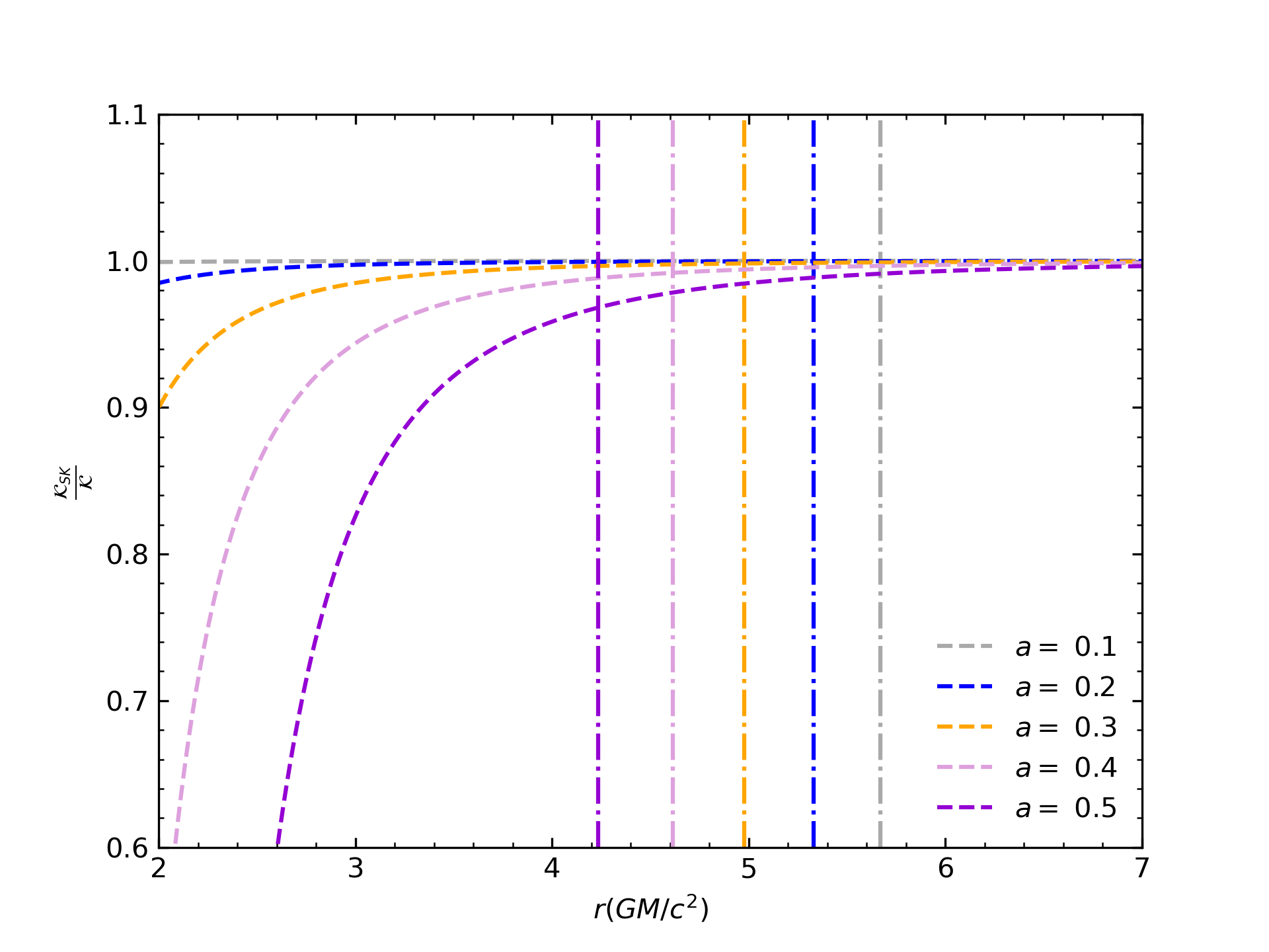
Figure 1: Ratio between the Kretschmann scalar in the slowly rotating Kerr metric and the standard Kerr metric, for different values of the spin parameter $a$, where vertical lines are the location of the ISCO for each $a$.

In Figure 2 we show the specific energy, angular momentum, Keplerian frequency and the effective potential from equations (53)-(56) for different values of the coupling $\alpha$. It can be noticed that as the value of $\alpha$ increases and approaches its upper limit, clearer differences appear in the Keplerian frequency, energy and specific angular momentum. As a test particle approaches the event horizon, when looking at the plots of the energy and specific angular momentum for values of $\alpha$ larger than $0.05$ it seems that an unstable circular orbit emerges near the horizon within the ISCO, as well as a more intricate behaviour in the Keplerian frequency.

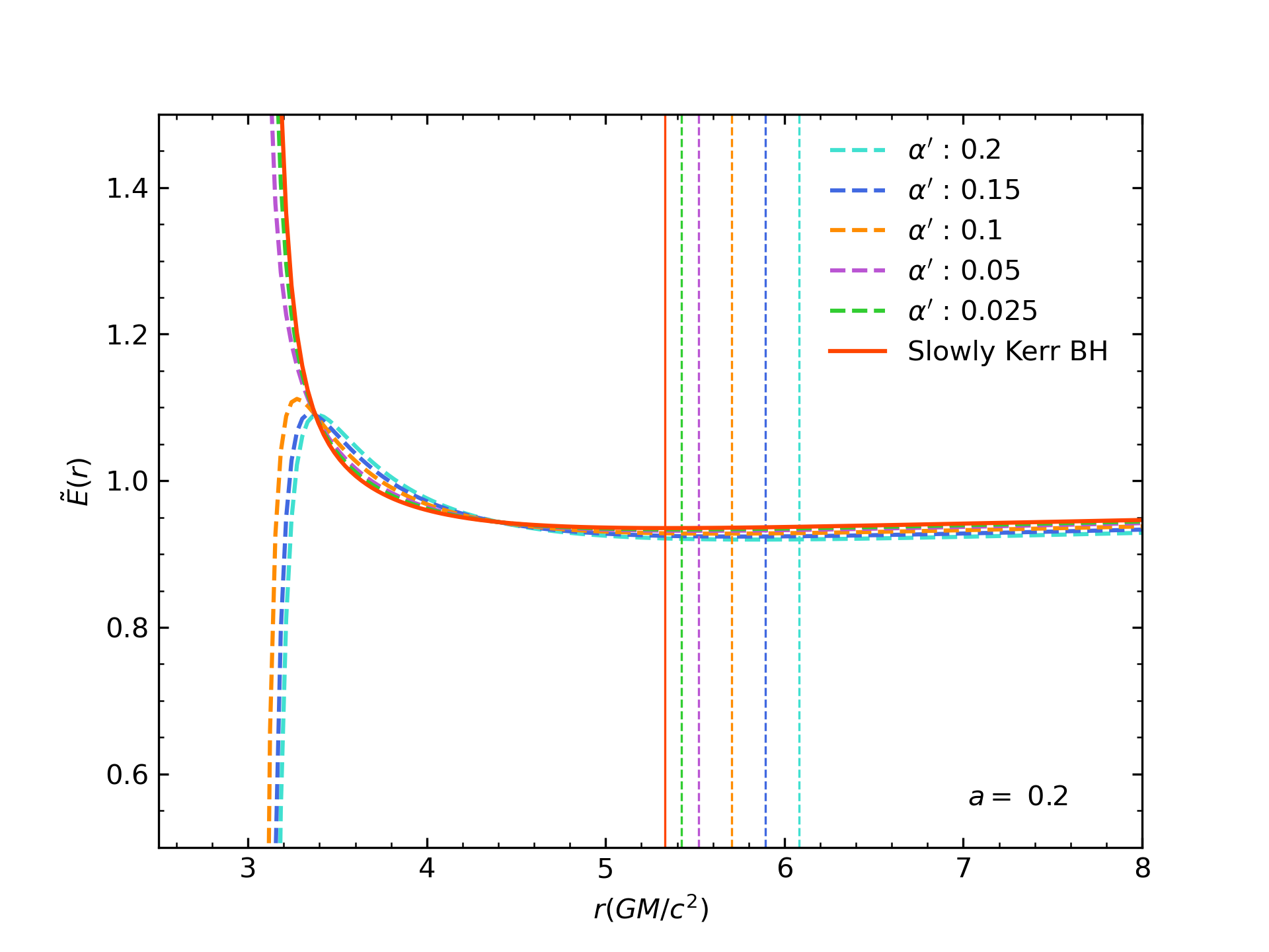
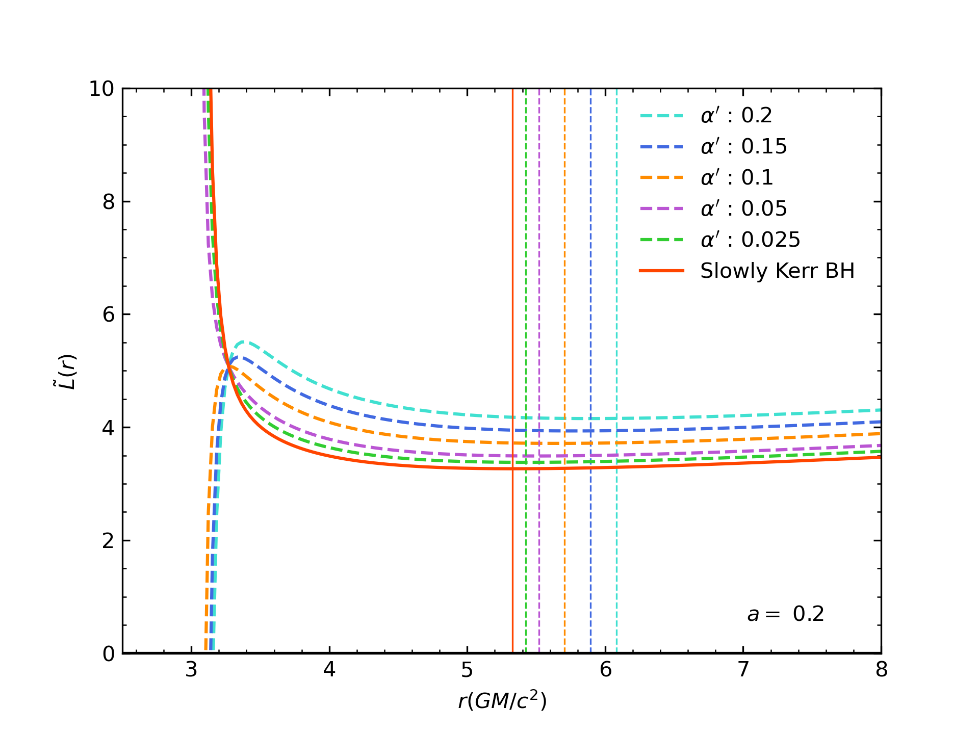
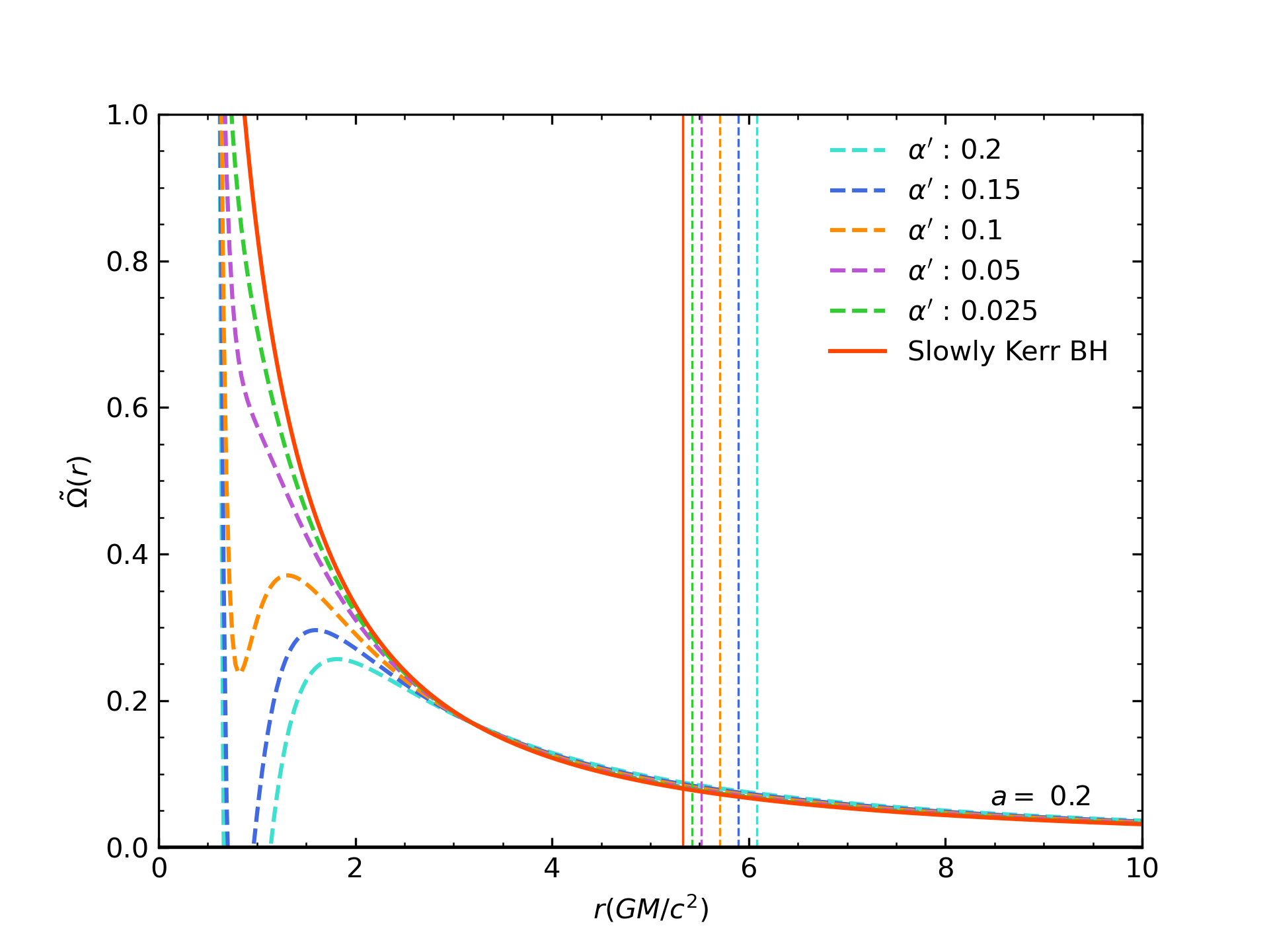
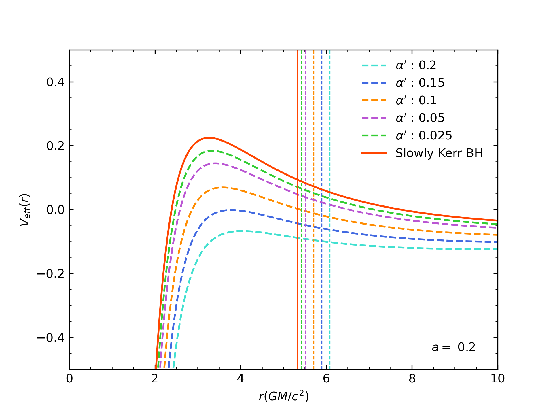
Figure 2: The upper-left panel shows the specific energy $\tilde{E}(r)$, the upper-right panel the specific angular momentum, the bottom-left panel the Keplerian frequency and the bottom-right panel shows the effective potential for the values of $E=1$ and $L=4.5$, for the $\alpha^{\prime}$-corrected BH with a mass of $M=6.2\times 10^{9}M_{\odot}$ and different values of $\alpha$ from $0$ to the upper limit $\sim 2$ in equation (38).

IV.5 Photon rings of slowly rotating $\alpha^{\prime}$-corrected black hole

We address now the problem of the separability of the Hamilton-Jacobi equation for null geodesics, namely

$$g^{\mu\nu}\frac{\partial S}{\partial x^{\mu}}\frac{\partial S}{\partial x^{\nu}} =0\,.$$ (61)

We assume a separable ansatz for the Jacobi characteristic function

$$S =-Et+L\phi+W(r)+P(\theta)\ .$$ (62)

Interestingly, equation (61) is compatible with the separable ansatz, leading to the following two equations

$$\left(\frac{\mathrm{d}P}{\mathrm{d}\theta}\right)^{2} +\frac{\xi^{2}}{\sin^{2}\theta}-a^{2}\cos^{2}\theta-\xi^{2}-\eta=0\,,$$ (63)

and

$$-\tilde{\Delta}\left(\frac{\mathrm{d}W(r)}{\mathrm{d}r}\right)^{2}+\frac{(\xi^{2}-4M^{2})r-2M\xi^{2}}{r(2M-r)^{2}}a^{2}+$$

$$+\left(\frac{4\xi(4M^{2}+3Mr-3r^{2})}{3r^{2}(2M-r)^{2}}\alpha-\frac{4M\xi}{2M-r}\right)a+$$

$$-\frac{2(12M^{3}+5M^{2}r+6r^{2}M-6r^{3})}{3(2M-r)^{2}M}\alpha+$$

$$+\frac{(r-2M)\xi^{2}-r^{3}}{2M-r}-\eta =0$$ (64)

where $\eta$ is the separation constant and we have defined $\xi\equiv\tilde{E}/L$ normalizing all the quantities respect to $\tilde{E}$. Without loss of generality, we fix $\tilde{E}=1$, and define

$$\tilde{\Delta} \equiv r^{2}-2Mr+a^{2}+\frac{-40M^{2}+6Mr+6r^{2}}{3r^{2}}\alpha\,.$$ (65)

From here we define the functions

$$R(r) \equiv\frac{\tilde{\Delta}^{2}}{\tilde{E}^{2}}\left(\frac{\mathrm{d}W(r)}{\mathrm{d}r}\right)^{2}\,,$$ (66)

$$\Theta(\theta) \equiv\frac{1}{\tilde{E}^{2}}\left(\frac{\mathrm{d}P(\theta)}{\mathrm{d}\theta}\right)^{2}\,.$$ (67)

Following these definitions the Jacobi characteristic functions is written as

$$S =-t+\xi\phi+\int_{r_{0}}^{r}\mathrm{d}r\frac{\sqrt{R(r)}}{\tilde{\Delta}}+\int_{\theta_{0}}^{\theta}\mathrm{d}\theta\sqrt{\Theta(\theta)}$$ (68)

and the first order equations for the non-trivial coordinates reduce to

$$g_{rr}^{2}\dot{r}^{2} =\frac{R(r)}{\tilde{\Delta}^{2}}\,,$$ (69)

$$g_{\theta\theta}^{2}\dot{\theta}^{2} =\Theta(\theta)$$ (70)

Then it is possible to find conditions for the existence of circular orbits without restricting to the equatorial plane, by imposing the following two conditions for all $r$

$$R(r) =0\,,$$ (71)

$$\frac{\mathrm{d}R(r)}{\mathrm{d}r} =0\,.$$ (72)

These equations can be solved in terms of the constants $\xi$ and $\eta$ giving two families of solutions. Considering the branch that connects with the Kerr solution perturbatively, we have

$$\xi =a\frac{M+r}{M-r}+\frac{r^{3}-3r^{2}}{a(M-r)}+$$ (73)

$$+\frac{a\alpha}{6r^{4}(2M-r)^{2}(M-r)M}(-240M^{7}+592M^{6}r+$$

$$+62M^{5}r^{2}-347M^{4}r^{3}+44M^{3}r^{4}+25M^{2}r^{5}+24Mr^{6}-12r^{7})+$$

$$+\frac{\alpha}{a}\frac{1}{3r(M-r)^{2}(2M-r)M}(-336M^{5}+327M^{4}r+$$

$$-66M^{3}r^{2}+16M^{2}r^{3}-18r^{4}M+3r^{5})$$

and

$$\eta =\frac{4Mr^{3}}{(M-r)^{2}}-\frac{(3M-r)^{2}r^{4}}{(M-r)^{2}a^{2}}+\frac{\alpha}{3r^{2}(M-r)^{3}(2M-r)^{2}}\times$$

$$\times(-720M^{7}+2016M^{6}r-118M^{5}r^{2}-1619M^{4}r^{3}$$

$$+781M^{3}r^{4}-47M^{2}r^{5}+21Mr^{6}-18r^{7})+$$

$$-\frac{\alpha}{a^{2}}\frac{2r(r-3M)}{(r-2M)(r-M)^{3}}(r^{5}-6r^{4}M+\frac{16}{3}M^{2}r^{3}+$$

$$-22M^{3}r^{2}+109M^{4}r-112M^{5}).$$ (74)

The impact parameters $x^{\prime}$ and $y^{\prime}$ defined as in Bardeen [15], are the usual Cartesian coordinates of the image plane for a observer located at $r=r_{0}$ coordinate distance and with inclination angle of view $\theta=i$. In the case of $r_{0}\rightarrow\infty$, the expression for the impact parameters are

$$x^{\prime} = -\frac{\xi}{\sin i},$$ (75)

$$y^{\prime} = \pm\sqrt{\Theta(i)},$$ (76)

where $\Theta(i)=a^{2}\cos^{2}i-\xi^{2}\cot i+\eta$.

The shape of the photon rings in the usual Kerr metric has been already studied previously by several authors Bardeen [15], Luminet [16], Takahashi [17], Beckwith and Done [18], Amarilla et al. [19], Johannsen [20], Giribet et al. [21]. Using the previous equations it is possible to obtain images of the photon rings in the slowly rotating $\alpha^{\prime}$-corrected metric (see Figure 3) in order to observe the effects of $\alpha$ in the shape of the photon ring and to compare it with the Kerr case.

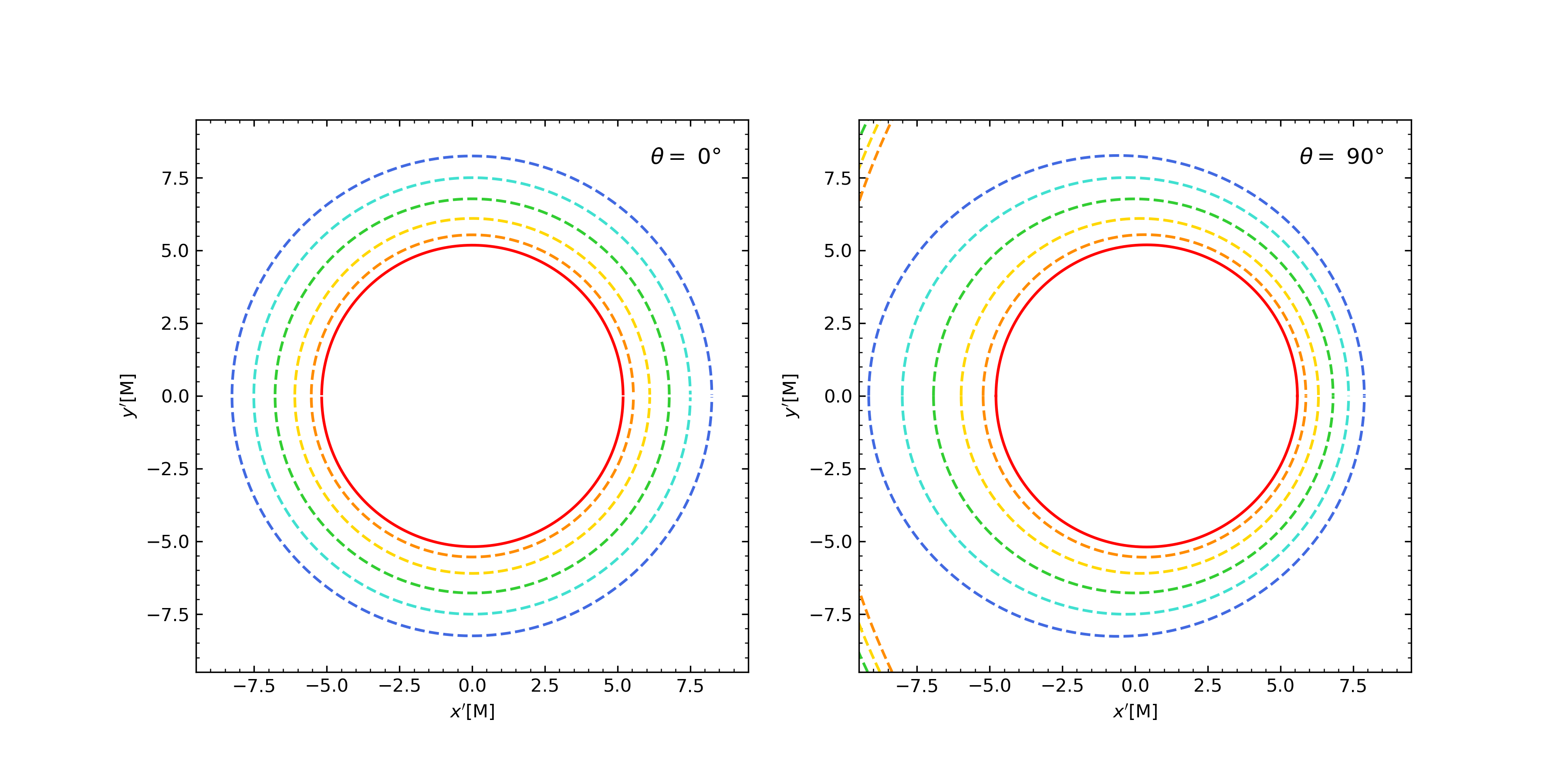
Figure 3: Photon rings around the $\alpha^{\prime}$-corrected black holes at an inclination angle of $\theta=i=0^{o}$ (left panel) and $i=90^{o}$ (right panel), where the (red line) represents a black hole with spin parameter $a=0.2M$ in the Kerr approximation. The (orange dashed line to blue dashed line) correspond to black holes with the coupling $\alpha=[0.04,0.08,0.12,0.16,0.2]$, respectively, in units of the gravitational radius squared $r_{g}^{2}$.

V Numerical model

In this section, we describe our numerical model, including the assumptions for the structure of the thin disk as well as the ray-tracing code RAPTOR I [22].

V.1 Thin-disk model

To analyze and obtain the shadow of the black hole, we assume a thin accretion disk, using the standard relativistic thin-disk model from Novikov and Thorne [23]. This model describes a geometrically thin disk with steady and axially symmetric states of the matter around the black hole. The distribution of the matter starts at the location of the ISCO radius and extends to some very large radius $r_{out}$, forcing the particles to move in nearly circular geodesics in the equatorial plane along the disk.

From the equations of conservation of energy, rest mass, and angular momentum in the disk paticles [23], the radiation flux emitted by the surface of the disk follows as

$$F(r)=\frac{\dot{M}}{4\pi M^{2}}f_{disk}(r),$$ (77)

where $\dot{M}$ is the mass accretion rate and

$$f_{disk}(r)=-\dfrac{d\Omega}{dr}\dfrac{M^{2}}{\sqrt{-g}(\tilde{E}-\Omega\tilde{L})^{2}}\int_{r_{in}}^{r}(\tilde{E}-\Omega\tilde{L})\dfrac{d\tilde{L}}{d\overline{r}}d\overline{r}$$ (78)

is a dimensionless function of the radius, $\Omega$ is the Keplerian frequency, $\tilde{E}$ and $\tilde{L}$ are the specific energy and angular momentum, $r_{in}$ is the location of the ISCO radius and $g$ is the determinant of the metric in cylindrical coordinates $(t,r,z,\phi)$. In the case of SK we have $\sqrt{-g}=r$ and for the metric defined in Eq. (11), one has

$$\sqrt{-g}=\sqrt{r^{2}-\alpha\left(\frac{32M^{2}+18Mr+12r^{2}}{3Mr}\right)}.$$ (79)

Figure 4 shows the flux for this space-time compared to the slowly rotating Kerr case, where it can be seen that as $\alpha$ grows the flux moves slightly outwards from the black hole.

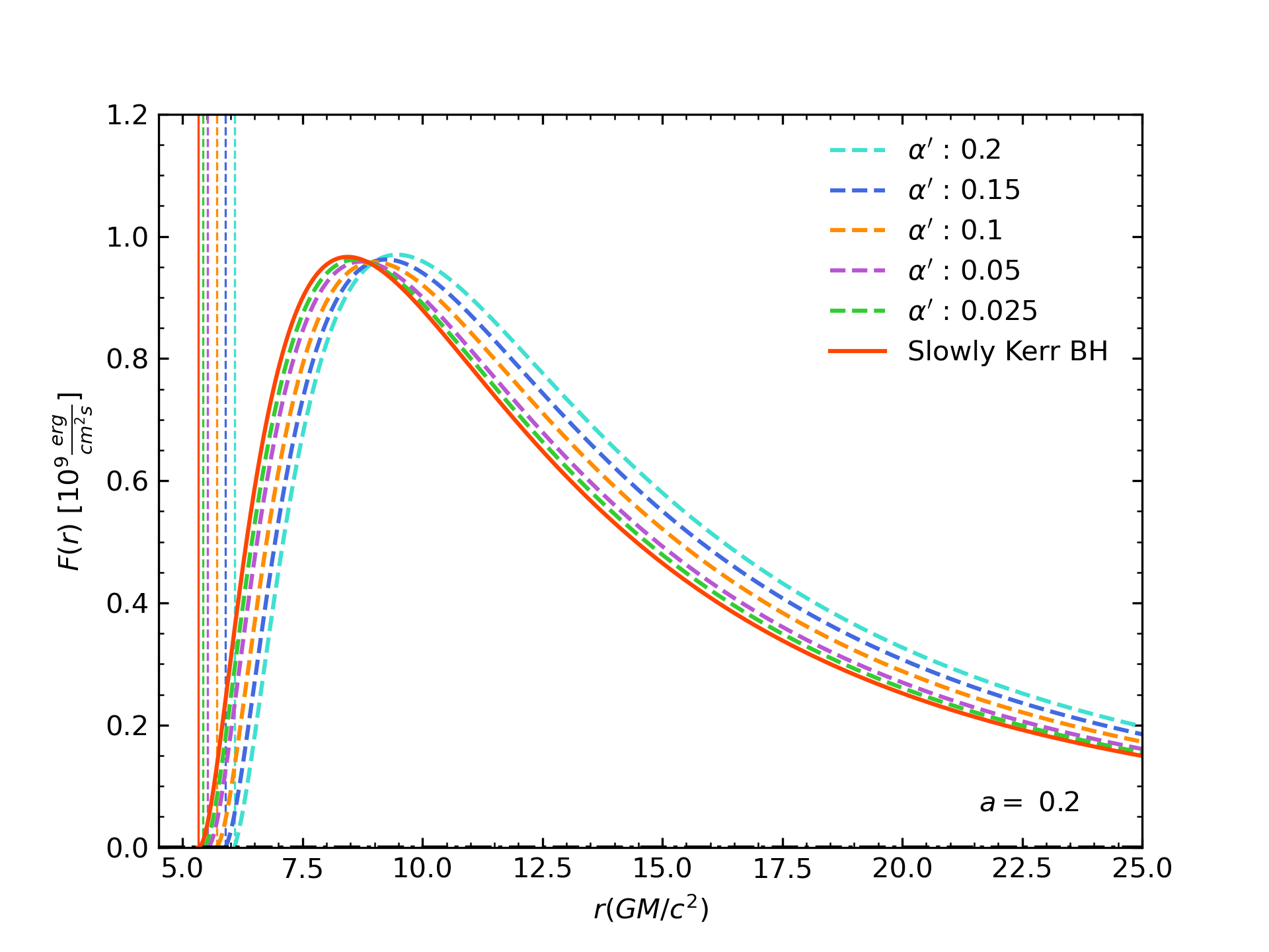
Figure 4: The energy flux of a BH with a rotation parameter $a=0.2M$, mass of $M_{BH}=6.2\times 10^{9}M_{\odot}$ and mass accretion rate $\dot{M}=1.172\times 10^{23}[g/s]$ [24] for different values of $\alpha$, where vertical lines represents the ISCO value for each $\alpha$.

Since the radiative description of this model is defined by thermal equilibrium black-body emission due to its simplicity and effectiveness, the flux is related to the disk temperature according to the standard Stefan-Boltzmann law as

$$F(r)=\sigma T_{eff}(r)^{4},$$ (80)

where $\sigma$ is the Stefan-Blotzmann constant and $T_{eff}(r)=f_{col}^{-1}T_{col}(r)$. Here the specific intensity can be defined as

$$I_{\nu}=\frac{1}{f_{col}^{4}}B_{\nu}(\nu,T_{col}),$$ (81)

where $f_{col}$ is the spectral hardening factor and

$$B_{\nu}(\nu,T_{col})=\dfrac{2h\nu^{3}}{c^{2}}\dfrac{1}{\exp(h\nu/k_{B}T_{col})-1}$$ (82)

is the Planck distribution for a blackbody spectrum. Here $\nu$ is the frequency of emission and $h$ and $k_{B}$ are the Planck and Boltzmann constants, respectively.

V.2 Ray-tracing code RAPTOR I

To obtain images of the BH shadow in the slowly rotating $\alpha^{\prime}$ space-time, we employ a modified version of the open-source ray tracing code RAPTOR I [22], which is capable to work in arbitrary space-times. The code calculates the null geodesic around the BH and solves the relativistic radiative transfer equation along the geodesics. To use it for obtaining images of BHs in this specific space-time, we modified the metric of the code, the connection and also included the thin accretion disk model [23] with the specific changes of the different physical quantities such as the location of the ISCO, the velocity of the disk and the flux emitted according to this model as we discussed in section V.1 for this space-time.

The code starts creating a virtual camera at a distant observer position to define the initial conditions for the light rays; this is performed following the general approach from Bambi [25].

Therefore, RAPTOR I integrates the geodesics along the path of the rays which interacts with the structure of the disk that extends from the ISCO radius (57) to $r_{out}=1000r_{g}$. In a final step the code employs the calculation of the radiative transfer equation at the observer’s location as

$$I_{\nu,obs}=\overline{g}^{3}I_{\nu},$$ (83)

where $I_{\nu}$ is the intensity emitted from Eq. (81) and $\overline{g}$ is the redshift factor

$$\overline{g}=\frac{\nu_{obs}}{\nu},$$ (84)

where $\nu_{obs}$ is the frequency at observer frame and

$$\nu=k^{\mu}u_{\mu}$$ (85)

is the frequency in the plasma frame, $k^{\mu}$ is the contravariant wave vector and $u_{\mu}$ is the covariant four-velocity.

VI Black hole simulations and shadow characterization

In the following, we present our simulation results with an analysis of the diameter, displacement and asymmetry of the obtained images.

VI.1 Diameter, displacement and asymmetry

To characterize the shadow of the different black holes in order to compare them, we employ the method used by [20, 26] that consists in the study of the peaks of the intensity profile in each image of the black hole to calculate the displacement, diameter and asymmetry through the following expressions. The displacement is defined as

$$D\equiv\frac{|x_{max}+x_{min}|}{2},$$ (86)

where $x_{max}$ and $x_{min}$ are the locations of the two peaks in the horizontal intensity profile. Analogously, it is possible to define the displacement in the vertical direction. Then the average radius is defined by

$$\langle\overline{R}\rangle\equiv\dfrac{1}{2\pi}\int_{0}^{2\pi}\overline{R}d\alpha,$$ (87)

where $\overline{R}\equiv\sqrt{(x^{\prime}-D_{x})^{2}+(y^{\prime}-D_{y})^{2}}$. Thus the diameter is $L=2\langle\overline{R}\rangle$.

Consequently, we get the following expression for the asymmetry:

$$A\equiv 2\sqrt{\dfrac{\int_{0}^{2\pi}\left(\overline{R}-\langle\overline{R}\rangle\right)^{2}d\alpha}{2\pi}}.$$ (88)

VI.2 Simulations

We performed simulations with RAPTOR I of an $\alpha^{\prime}$-corrected BH that are shown in Figure 5, with mass similar to M87*, for a thin accretion disk model. The settings of the simulations are shown in Table 1.

Table 1: Setup for the simulation, values extracted from Akiyama et al. [24]

Variable	​​​​ Value
Mass	$6.2\times 10^{9}$ $\mathrm{M_{\odot}}$
Distance	$16.9$ $\mathrm{Mpc}$
$a$	$0.2\ M$
$r_{\text{camera}}$	$10^{4}\ \mathrm{r_{g}}$
Range for $(x^{\prime}$, $y^{\prime})$	$[-20,20]\ \mathrm{r_{g}}$
Resolution $(x,y)$	$200$ $\mathrm{px}$
Frequency	$230$ $\mathrm{GHz}$
Inclination (°)	$[0,30,60,90]$
$\dot{M}$	$1.71\times 10^{23}\mathrm{g/s}$
$\alpha^{\prime}$	$[0,0.1,0.15,0.2]$

To compare the shadow and disk structure of this BH with the usual Kerr BH in the same physical conditions, we performed a similar analysis as Agurto-Sepulveda et al. [26], calculating the intensity profile of each image, for different viewing angles from face-on to edge-on and then we obtained the values of the diameter, displacement and asymmetry of the shadow from equations (86-88) for each simulation.

A comparison is shown in Figure 6, where one can see that an increasing value of $\alpha^{\prime}$ leads to an increase of the diameter of the image compared to Kerr while it decreases when going from a face-on to an edge-on viewing angle. Here, it is also important to notice that the Kerr case and the slowly rotating Kerr case also differ in the diameter for a few values of inclination. In the case of the displacement, we can see a similar situation, where the displacement of the shadow increases with the value of $\alpha^{\prime}$, and decreases abruptly for an edge-on viewing angle. Here, the difference between the Kerr case and the $\alpha^{\prime}$-corrected case is also clearly visible. Finally, the asymmetry values do not differ as much as their predecessors and are quite close to the Kerr case, yet for increasing $\alpha^{\prime}$ differences can be noticed for the first lower half of the viewing angles and stay close to Kerr’s case for the top half.

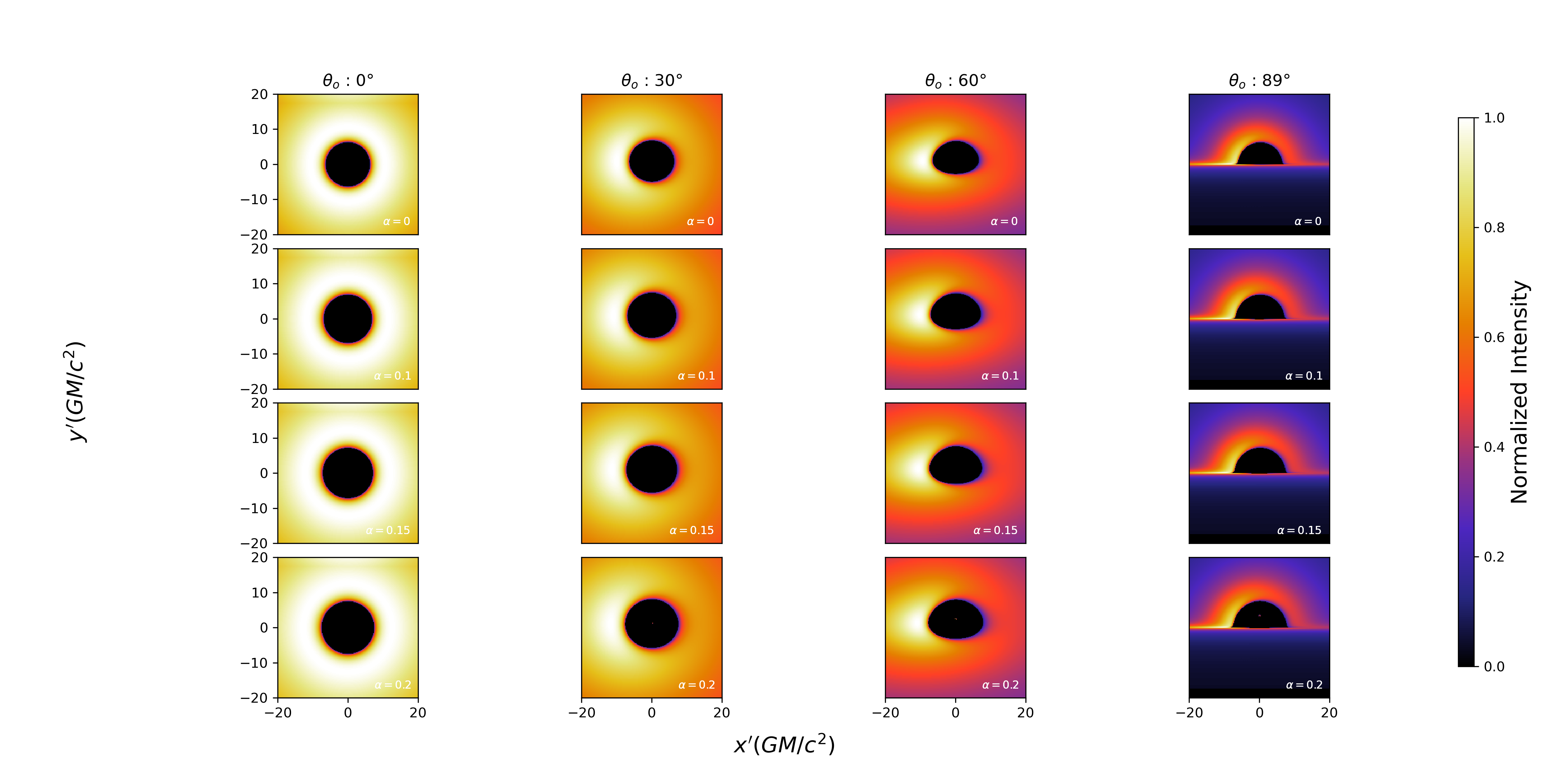
Figure 5: Simulation performed by Raptor I code of the Novikov-Thorne thin accretion disk model for a slowly rotating $\alpha^{\prime}$-corrected SMBH with a mass of $M=6.2\times 10^{9}M_{\odot}$, a mass accretion rate of $\dot{M}=1.172\times 10^{23}[g/s]$, a spin parameter $a=0.2M$ and couplings $\alpha=[0.1,0.15,0.2]$, in units of the $r_{g}^{2}$.

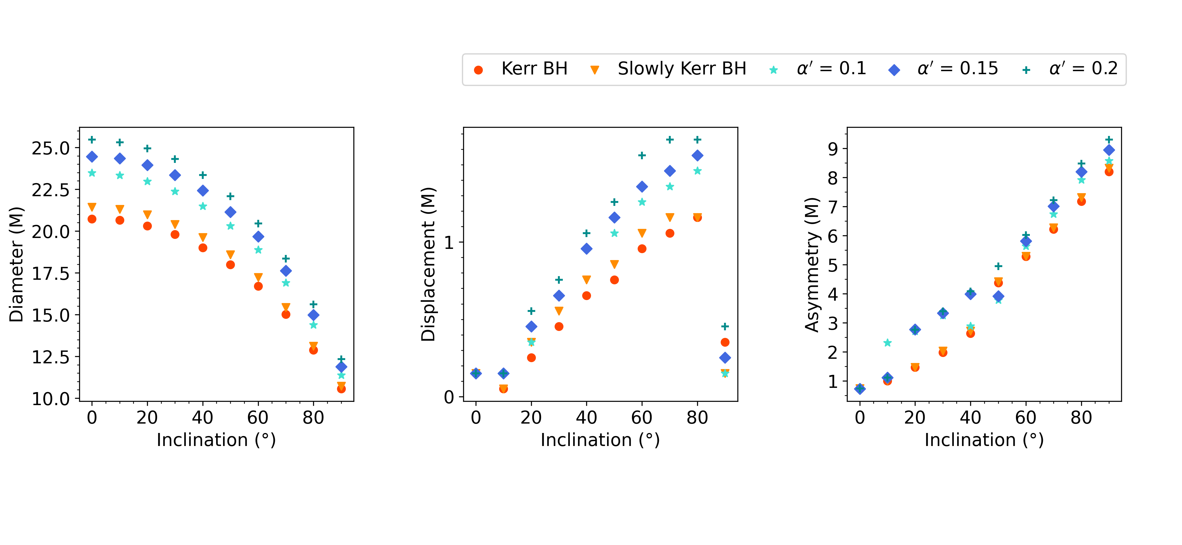
Figure 6: Comparison of the diameter, displacement and asymmetry values, for simulations of Kerr space-time (red dots), slowly rotating Kerr approximation (orange triangles) and $\alpha^{\prime}$-corrected BH with different values of the coupling term $\alpha=[0.1,0.15,0.2]\ r_{g}^{2}$ (cyan stars, blue diamonds and darkcyan plus sign, respectively).

VI.3 Effects of $\alpha^{\prime}$-corrected terms in the shadow

One way to observe possible signals of the deviations from the Kerr shadow due to the $\alpha^{\prime}$-corrected terms, is setting the structure of the disk from a given value of ISCO radius $r_{isco}$ to a big outer radius $r_{out}$ for the two different space-times in the simulations.

As we have seen before, increasing the value of $\alpha^{\prime}$ correspond to an increase in the diameter and displacement of the BH shadow. Since $\alpha^{\prime}$ stands for the inverse of the tension of the string, it must be positive. Therefore, to have a same value for the ISCO radius with different values of $\alpha^{\prime}$ and spin parameter $a$ we proceed as follows: we fix the ISCO radius as $r_{isco}=7.31r_{g}$, which in Kerr metric yields a value of spin parameter $a=-0.42M$, while in the slowly rotating $\alpha^{\prime}$ metric yields a spin parameter $a=-0.3M$ and the coupling value of $\alpha=0.189\ r_{g}^{2}$.

Figure 7 shows the difference between the two images of a Kerr black hole (left panel) and the slowly rotating $\alpha^{\prime}$-corrected black hole (right panel) with the same location of the ISCO corresponding to the previously described setting. A careful look at the images shows a slight difference in the shadow size, being larger in the case of $\alpha^{\prime}-$corrected space-time, as well as a slight difference in the intensity of the images.

In Figure 8 we show the differences in the diameter, displacement and asymmetry values for different angles of view for the same configuration, including also a comparison with the slowly rotating Kerr spacetime. There, it is possible to notice a greater difference between the images. The $\alpha^{\prime}$-corrected BH shows a bigger diameter compared to the Kerr BH, for an angle of view near face-on, while the diameters get closer as one approaches the edge angle. In the case of the displacement, it is clearly seen that for increasing angle of view the displacement also increase for the $\alpha^{\prime}$-corrected BH, when compared to the Kerr BH. In the case of asymmetry, the difference between the two images seems to be less clear, a slight difference may be visible for an angle of view closer to the edge-on, but still the values seem to be close to each other.

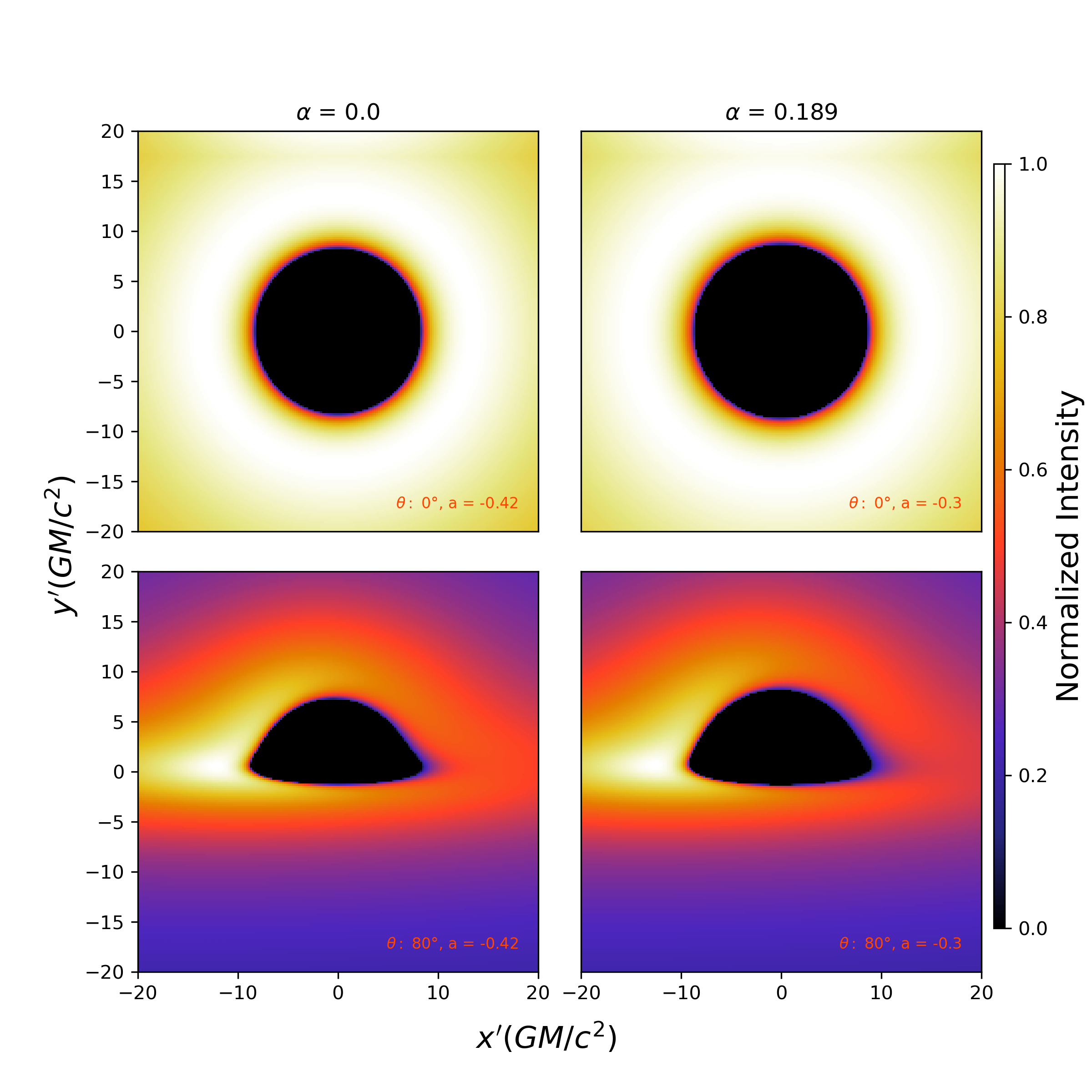
Figure 7: Comparison between two simulations with the similar configuration of Table 1 for a BH in a Kerr space-time (left panel) with a spin parameter $a=-0.42M$ and inclination angle of view $\theta=[0,80]$ degrees and a slowly rotating $\alpha^{\prime}$-corrected BH (right panel) with different values of the coupling term $\alpha=0.189\ r_{g}^{2}$ and spin parameter $a=-0.3M$.

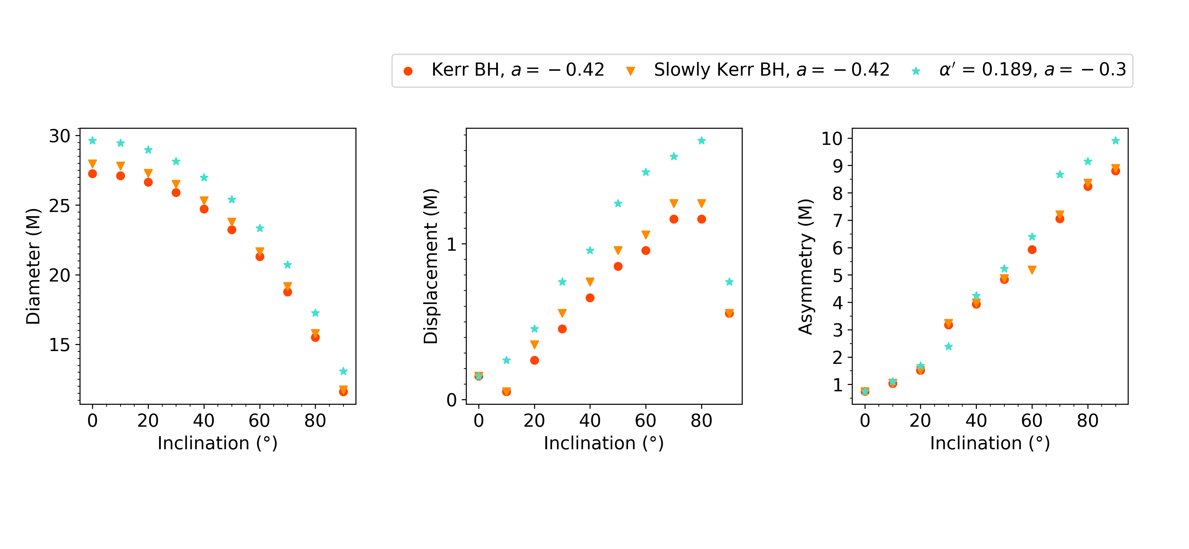
Figure 8: Comparison of the diameter, displacement and asymmetry values, for simulations of BHs with the same ISCO radius in the Kerr space-time (red dots) and slowly rotating Kerr approximation (orange triangles) with a retrograde spin parameter $a=-0.42M$ and $\alpha^{\prime}$-corrected BH with a spin parameter $a=-0.3M$ and $\alpha^{\prime}=0.189$.

Table 2 shows several simulations with the same approach, fixing the ISCO radius, which were performed to observe the effect of $\alpha^{\prime}$ for different values of spin $a$ and the same angle of view of $75^{o}$.

Table 2: Comparison between the diameter, displacement and asymmetry for a set of simulations with the same ISCO radius and different values of the spin parameter $a$ and the coupling $\alpha^{\prime}$.

​​$r_{isco}\ [\mathrm{r_{g}}]$	​​ $a\ [\mathrm{M}]$	​​$\alpha^{\prime}[\mathrm{r_{g}^{2}}]$	​​ $L\ [\mathrm{r_{g}}]$	​​ $D\ [\mathrm{r_{g}}]$	​​ $A\ [-]$	​​ $\theta\ [{}^{o}$]
	$-0.05$	$0$	$15.389$	$1.158$	$7.121$
$6.162$	$0.05$	$0.102$	$16.481$	$1.461$	$7.555$	$75$
	$0.1$	$0.145$	$16.816$	$1.561$	$7.753$
	$0.15$	$0.185$	$17.105$	$1.561$	$7.857$
	$-0.1$	$0$	$15.642$	$1.057$	$7.167$
$6.322$	$-0.05$	$0.056$	$16.375$	$1.360$	$7.472$	$75$
	$0.05$	$0.152$	$17.146$	$1.561$	$7.814$
	$0.1$	$0.193$	$16.415$	$1.662$	$8.581$
	$-0.15$	$0$	$15.883$	$1.158$	$7.258$
$6.481$	$-0.1$	$0.059$	$16.705$	$1.360$	$7.583$	$75$
	$-0.05$	$0.112$	$17.151$	$1.461$	$7.774$
	$0.05$	$0.201$	$17.647$	$5.088$	$9.524$
	$-0.2$	$0$	$16.143$	$1.158$	$7.358$
$6.639$	$-0.15$	$0.063$	$17.031$	$1.360$	$7.680$	$75$
	$-0.1$	$0.119$	$17.419$	$1.461$	$7.855$
	$-0.05$	$0.168$	$17.733$	$1.662$	$8.035$
	$-0.3$	$0$	$16.659$	$1.158$	$7.502$
$6.949$	$-0.25$	$0.074$	$17.590$	$1.360$	$7.849$	$75$
	$-0.2$	$0.136$	$18.039$	$1.662$	$8.054$
	$-0.15$	$0.189$	$18.459$	$1.662$	$8.268$
	$-0.4$	$0$	$17.153$	$1.158$	$7.639$
$7.254$	$-0.3$	$0.160$	$18.773$	$1.561$	$8.268$	$75$

Our results indicate that there are particular observable quantities, for which the differences on the BH image, for a given ISCO, are enhanced and therefore one could look for such observables to obtain a greater difference, when looking for qualitative signals beyond GR, in the context of the $\alpha^{\prime}$-corrected black holes.

VII Conclusions and discussions

Summarizing, the solution that we presented in this paper is a extension of our slowly rotating solution described in [12], including the logarithmic branch from the static solution. We presented the conserved charges, the Hawking temperature and the entropy for this space-time in the particular case of $b=0$. Then, we studied several properties of the metric, first we assign a Petrov D type to the solution, we found a curvature singularity inside the event horizon, the location of the event horizon and ergosphere, as well as an upper limit for $\alpha$, all the quantities related to the Kerr metric. We then move on to the study of circular geodesics motion of test particles where we find that the circular orbits around this black hole are different from the Kerr orbit, presenting an unstable circular orbit close to the horizon. We also find that our solution is separable under the Hamilton-Jacobi equations, allowing us to find expressions for the photon rings where it is possible to see that as $\alpha$ grows, the ring diameter grows as well. Finally, we move on to the study of black hole shadowing by means of numerical ray tracing simulations for a thin accretion disc, and then a post-analysis is carried out. Determining that increasing values of $\alpha$ increase the diameter of the shadow and subtly affect the shadow offset and asymmetry. This is evident from simulations where the accretion disc has the same starting point, i.e. the same ISCO radius.

References

• Abbott et al. [2016] B. P. Abbott, R. Abbott, T. Abbott, M. Abernathy, F. Acernese, K. Ackley, C. Adams, T. Adams, P. Addesso, R. X. Adhikari, et al., Observation of gravitational waves from a binary black hole merger, Physical review letters 116, 061102 (2016).
• Collaboration et al. [2019] E. H. T. Collaboration, K. Akiyama, A. Alberdi, W. Alef, K. Asada, R. Azuly, et al., First m87 event horizon telescope results. i. the shadow of the supermassive black hole, Astrophys. J. Lett 875, L1 (2019).
• Akiyama et al. [2022] K. Akiyama, A. Alberdi, W. Alef, J. C. Algaba, R. Anantua, K. Asada, R. Azulay, U. Bach, A.-K. Baczko, D. Ball, et al., First sagittarius a* event horizon telescope results. i. the shadow of the supermassive black hole in the center of the milky way, The Astrophysical Journal Letters 930, L12 (2022).
• Collaboration et al. [2021] E. H. T. Collaboration et al., First m87 event horizon telescope results. viii. magnetic field structure near the event horizon, arXiv preprint arXiv:2105.01173  (2021).
• Akiyama et al. [2023] K. Akiyama et al. (EHT), First M87 Event Horizon Telescope Results. IX. Detection of Near-horizon Circular Polarization, Astrophys. J. Lett. 957, L20 (2023)arXiv:2311.10976 [astro-ph.HE] .
• Akiyama et al. [2024] K. Akiyama, A. Alberdi, W. Alef, J. C. Algaba, R. Anantua, K. Asada, R. Azulay, U. Bach, A.-K. Baczko, D. Ball, et al., First sagittarius a* event horizon telescope results. vii. polarization of the ring, The Astrophysical Journal Letters 964, L25 (2024).
• Note [1] The ngEHT web: https://www.ngeht.org/.
• Ricarte et al. [2022] A. Ricarte, P. Tiede, R. Emami, A. Tamar, and P. Natarajan, The ngeht’s role in measuring supermassive black hole spins, Galaxies 11, 6 (2022).
• Metsaev and Tseytlin [1987a] R. R. Metsaev and A. A. Tseytlin, Order alpha-prime (Two Loop) Equivalence of the String Equations of Motion and the Sigma Model Weyl Invariance Conditions: Dependence on the Dilaton and the Antisymmetric Tensor, Nucl. Phys. B 293, 385 (1987a).
• Metsaev and Tseytlin [1987b] R. R. Metsaev and A. A. Tseytlin, Two loop beta function for the generalized bosonic sigma model, Phys. Lett. B 191, 354 (1987b).
• Maeda et al. [2012] K.-i. Maeda, N. Ohta, and R. Wakebe, Accelerating Universes in String Theory via Field Redefinition, Eur. Phys. J. C 72, 1949 (2012)arXiv:1111.3251 [hep-th] .
• Agurto-Sepúlveda et al. [2023] F. Agurto-Sepúlveda, M. Chernicoff, G. Giribet, J. Oliva, and M. Oyarzo, Slowly rotating and accelerating $\alpha$’-corrected black holes in four and higher dimensions, Phys. Rev. D 107, 084014 (2023)arXiv:2207.13214 [hep-th] .
• Cano and Ruipérez [2022] P. A. Cano and A. Ruipérez, String gravity in D=4, Phys. Rev. D 105, 044022 (2022)arXiv:2111.04750 [hep-th] .
• Wald [1993] R. M. Wald, Black hole entropy is the Noether charge, Phys. Rev. D 48, R3427 (1993)arXiv:gr-qc/9307038 .
• Bardeen [1973] J. Bardeen, Black holes ed c. dewitt and bs dewitt (1973).
• Luminet [1979] J.-P. Luminet, Image of a spherical black hole with thin accretion disk, Astronomy and Astrophysics, vol. 75, no. 1-2, May 1979, p. 228-235. 75, 228 (1979).
• Takahashi [2004] R. Takahashi, Shapes and positions of black hole shadows in accretion disks and spin parameters of black holes, The Astrophysical Journal 611, 996 (2004).
• Beckwith and Done [2005] K. Beckwith and C. Done, Extreme gravitational lensing near rotating black holes, Monthly Notices of the Royal Astronomical Society 359, 1217 (2005).
• Amarilla et al. [2010] L. Amarilla, E. F. Eiroa, and G. Giribet, Null geodesics and shadow of a rotating black hole in extended chern-simons modified gravity, Physical Review D 81, 124045 (2010).
• Johannsen [2013a] T. Johannsen, Photon rings around kerr and kerr-like black holes, The Astrophysical Journal 777, 170 (2013a).
• Giribet et al. [2023] G. Giribet, E. R. de Celis, and P. Schmied, Sub-annular structure in black hole image from gravitational refraction, arXiv preprint arXiv:2311.06388  (2023).
• Bronzwaer et al. [2018] T. Bronzwaer, J. Davelaar, Z. Younsi, M. Mościbrodzka, H. Falcke, M. Kramer, and L. Rezzolla, Raptor-i. time-dependent radiative transfer in arbitrary spacetimes, Astronomy & Astrophysics 613, A2 (2018).
• Novikov and Thorne [1973] I. D. Novikov and K. S. Thorne, Astrophysics of black holes, Black holes (Les astres occlus) 1, 343 (1973).
• Akiyama et al. [2019] K. Akiyama, A. Alberdi, W. Alef, K. Asada, R. Azulay, A.-K. Baczko, D. Ball, M. Baloković, J. Barrett, D. Bintley, et al., First m87 event horizon telescope results. v. physical origin of the asymmetric ring, The Astrophysical Journal Letters 875, L5 (2019).
• Bambi [2017] C. Bambi, Black holes: a laboratory for testing strong gravity, Vol. 10 (Springer, 2017).
• Agurto-Sepulveda et al. [2023] F. Agurto-Sepulveda, J. H. Lagunas, J. Pedreros, B. Bandyopadhyay, and D. R. G. Schleicher, Exploring how deviations from the Kerr metric can affect SMBH images,   (2023), arXiv:2309.11280 [gr-qc] .
• Johannsen [2013b] T. Johannsen, Systematic study of event horizons and pathologies of parametrically deformed kerr spacetimes, Physical Review D 87, 124017 (2013b).
• Thornburg [2007] J. Thornburg, Event and apparent horizon finders for 3+ 1 numerical relativity, Living Reviews in Relativity 10, 1 (2007).