Mapping the SMEFT at High-Energy Colliders:
from LEP and the (HL-)LHC to the FCC-ee

Abstract

We present SMEFiT3.0, an updated global SMEFT analysis of Higgs, top quark, and diboson production data from the LHC complemented by electroweak precision observables (EWPOs) from LEP and SLD. We consider recent inclusive and differential measurements from the LHC Run II, alongside with a novel implementation of the EWPOs based on independent calculations of the relevant EFT contributions. We estimate the impact of HL-LHC measurements on the SMEFT parameter space when added on top of SMEFiT3.0, through dedicated projections extrapolating from Run II data. We quantify the significant constraints that measurements from two proposed high-energy circular $e^{+}e^{-}$ colliders, the FCC-ee and the CEPC, would impose on both the SMEFT parameter space and on representative UV-complete models. Our analysis considers projections for the FCC-ee and the CEPC based on the latest running scenarios and includes $Z$-pole EWPOs, fermion-pair, Higgs, diboson, and top quark production, using optimal observables for both the $W^{+}W^{-}$ and the $t\bar{t}$ channels. The framework presented in this work may be extended to other future colliders and running scenarios, providing timely input to ongoing studies towards future high-energy particle physics facilities.

1 Introduction

The vast amount of data collected by the LHC during Run II has significantly increased our knowledge of fundamental particle physics. A global interpretation of these measurements is required to understand how well our best current theory, the Standard Model (SM), describes nature at the TeV scale and how much room (and where) is left for its extensions. The magnitude of this task, as well as our knowledge, keeps increasing thanks to the ongoing LHC Run III, which will provide exciting new insights.

Following Run III of the LHC, its High-Luminosity upgrade (HL-LHC) Cepeda:2019klc ; Azzi:2019yne is scheduled to start in 2029 and operate for the next decade, accumulating a total integrated luminosity of up to 3 ab^-1 per experiment. Beyond the HL-LHC program, several proposals for future particle colliders have been put forward and are being actively discussed by the global community. These proposals include electron-positron colliders, either circular such as the FCC-ee FCC:2018byv ; FCC:2018evy and the CEPC CEPCPhysicsStudyGroup:2022uwl , or linear such as the ILC Behnke:2013xla ; ILC:2013jhg , the C3 Vernieri:2022fae , and CLIC Linssen:2012hp , high-energy proton-proton colliders such as the FCC-hh FCC:2018byv ; FCC:2018vvp and the SppC Tang:2015qga , muon colliders Accettura:2023ked ; Aime:2022flm , and high-energy electron-proton/ion colliders such as the LHeC and the FCC-eh LHeC:2020van ; FCC:2018byv . Furthermore, with a focus on QCD and hadronic physics but also with a rich program of electroweak measurements and BSM searches, the Electron Ion Collider (EIC) AbdulKhalek:2021gbh has already been approved and is expected to see its first collisions in the early 2030s.

These proposed facilities envisage a significant expansion of our knowledge of nature at the smallest accessible scales. Novel insights would be provided via unprecedented sensitivity to subtle quantum effects, distorting the properties of known particles, and via the direct production of new particles, for instance, heavy (TeV-scale) particles or lighter ones but feebly interacting. While opening unique opportunities, the theoretical interpretation of future collider measurements also poses several challenges that must be tackled beforehand. In the specific case of leptonic colliders, significant theoretical progress both within the SM and beyond would be required to match the expected precision of the experimental measurements. This is illustrated with the Tera-$Z$ running program TLEPDesignStudyWorkingGroup:2013myl of circular $e^{+}e^{-}$ colliders, which would lead to up to $10^{12}$ $Z$-bosons at the FCC-ee, with hence extremely small statistical uncertainties.

Making an informed decision about which of these future particle colliders should be built demands, in addition to feasibility and cost/effectiveness studies, the quantitative assessment of their scientific reach. Several dedicated studies comparing the reach of future colliders have been presented in the last years, in particular in the context of the European Strategy for Particle Physics Update (ESPPU) EuropeanStrategyforParticlePhysicsPreparatoryGroup:2019qin and of the Snowmass US-based community process Narain:2022qud . The latter has recently culminated in the P5 report, one of whose main recommendations is endorsing an off-shore Higgs factory located in either Europe or Japan. As the European community ramps up its activities towards the next update of its long-term strategy, continuing, diversifying, and deepening these quantitative assessments of the reach of future colliders is more timely than ever.

The Standard Model Effective Field Theory (SMEFT) framework Grzadkowski:2010es ; Brivio:2017vri ; Isidori:2023pyp is particularly well suited to perform global interpretations of current data and study the physics potential of future colliders. This feature follows from its ability to parametrize simultaneously the effects of a vast family of models of New Physics (NP) and to correlate effects in several observables. The models that are covered by the SMEFT are those where all new particles are heavier than the electroweak scale and that decouple from the SM  Falkowski:2019tft ; Cohen:2020xca . Hence, projected global SMEFT fits allow us to compare the proposed future colliders in generic NP scenarios. The development of flexible and user-friendly frameworks for such global interpretations is thus a timely priority Ellis:2020unq ; Brivio:2021alv ; Giani:2023gfq . Furthermore, the predictions computed within the SMEFT framework can then be reused to repeat the comparison within specific UV models by imposing the constraints dictated by the UV matching onto the SMEFT deBlas:2017xtg ; DasBakshi:2018vni ; Ellis:2020unq ; Brivio:2021alv ; Carmona:2021xtq ; Fuentes-Martin:2022jrf ; terHoeve:2023pvs .

The advantages of using SMEFT (and EFTs in general) for the assessment of future colliders have been leveraged by several groups in the past. First, in studies that considered a limited set of measurements and then in fits to a much larger data set, see e.g. Ellis:2015sca ; deBlas:2016nqo ; Ellis:2017kfi ; Durieux:2017rsg ; Barklow:2017suo ; Barklow:2017awn ; DiVita:2017vrr ; Chiu:2017yrx ; Durieux:2018tev ; deBlas:2019rxi ; DeBlas:2019qco ; LCCPhysicsWorkingGroup:2019fvj ; Jung:2020uzh ; deBlas:2021jlt ; MuonCollider:2022xlm ; deBlas:2022ofj ; Allwicher:2023shc . The latter group of studies has highlighted the need for the inclusion of LEP and SLD data and HL-LHC projections to avoid overestimating the benefits of future colliders deBlas:2019rxi ; DeBlas:2019qco ; deBlas:2022ofj . SMEFT studies at future lepton colliders could also probe some of the fundamental principles underlying Quantum Field Theory such as unitarity, locality and Lorentz invariance Gu:2020thj ; Gu:2020ldn .

A key component of the LEP and SLD legacy are the electroweak precision observables (EWPOs) ALEPH:2005ab from electron-positron collisions at the $Z$-pole and beyond. The high precision achieved by the measurements of EWPOs imposes stringent stress tests of the Standard Model (SM) Altarelli:1991fk ; Baak:2012kk and indirectly constrains a wide range of models beyond the Standard Model (BSM). Indeed, as compared to measurements at the LHC, these EWPOs provide complementary, and in many cases dominant, sensitivity to a wealth of BSM scenarios. In this respect, the EWPOs supplement uniquely the direct information on the properties of the Higgs and electroweak sectors obtained at the LHC Dawson:2018dcd ; Butter:2016cvz ; Azatov:2019xxn . In the language of the SMEFT, EWPOs provide information on several directions in the EFT parameter space Brivio:2017bnu , some of them of great relevance when matching onto compelling UV-completions terHoeve:2023pvs . However, the implementation of EWPOs within a SMEFT fit must deal with several theoretical subtleties, and ensure that the underlying settings such as the choice of electroweak input scheme, flavour assumptions, and operator basis are consistent with those adopted in the associated interpretation of LHC measurements.

The goal of this paper is two-fold. First, we present SMEFiT3.0, an updated global SMEFT analysis of Higgs, top quark, and diboson data from the LHC complemented by EWPOs from LEP and SLD. This analysis, carried out within the SMEFiT framework Hartland:2019bjb ; Ethier:2021ydt ; Ethier:2021bye ; vanBeek:2019evb ; Giani:2023gfq ; terHoeve:2023pvs , considers recent inclusive and differential measurements from the LHC Run II, in several cases based on its full integrated luminosity, alongside with a new implementation of the EWPOs. The latter is based on independent calculations of the relevant EFT contributions, ensures consistent theory settings between the $e^{+}e^{-}$ and hadron collider processes, and is benchmarked with previous studies in the literature. Constraining 45 (50) independent directions in the parameter space within linear (quadratic) SMEFT fits, this analysis provides a state-of-the-art set of EFT bounds enabled by available LEP and LHC data.

Second, starting from this SMEFiT3.0 baseline, we quantify the constraints on the EFT operators of projected measurements, first from the HL-LHC and subsequently from two of the proposed high-energy electron-positron colliders, namely the circular variants FCC-ee and the CEPC. This result is achieved by extending the SMEFiT framework with novel functionalities streamlining the inclusion of projections for future experimental facilities into the global fit. Beyond its specific application to FCC-ee and CEPC projections, this proof-of-concept study illustrates the relevance of SMEFiT for ongoing studies assessing the physics reach of new particle colliders. As such, we expect that it will represent a useful tool for the particle physics community in the ongoing discussions towards charting its long-term future. Our framework is open-source, extensively documented, and user-friendly. We provide all the inputs needed to reproduce our results, such that the community can easily reuse and expand them towards other future experiments.

Our analysis emphasises the profound interplay between measurements at leptonic and hadronic colliders to constrain complementary directions in the EFT parameter space. It illustrates the potential of future colliders, first the HL-LHC and then the FCC-ee and CEPC, to inform indirect BSM searches via high-precision measurements extending the sensitivity provided by existing data. This unprecedented reach is quantified both at the level of Wilson coefficients as well as in terms of the parameters (masses and couplings) of representative UV-complete models, in the latter case benefiting from progress in the interfacing with automated matching tools Carmona:2021xtq ; Fuentes-Martin:2022jrf , as presented in terHoeve:2023pvs .

The outline of this paper is as follows. First, in Sect. 2 we describe the new implementation of EWPOs in SMEFiT and benchmark our results with related studies in the literature. Sect. 3 presents the SMEFiT3.0 global analysis, including the LHC Run II measurements alongside the new EWPO implementation. By extrapolating from Run II data, this fit is used as a baseline to estimate the constraints on the SMEFT coefficients which may be achieved at the HL-LHC. In Sect. 4, projections for FCC-ee and CEPC measurements are added to the HL-LHC baseline to determine the ultimate sensitivity of future circular $e^{+}e^{-}$ colliders to the SMEFT parameter space. Sect. 5 presents the results of our global analyses of LHC Run II, HL-LHC and FCC-ee measurements at the level of the couplings and masses of UV-complete models matched onto the SMEFT. Finally, we summarise and outline possible developments in Sect. 6.

Technical information is collected in the appendices. App. A collects the input settings adopted for the SMEFT fits presented in this work. App. B describes the EFT operator basis adopted, whilst App. C describes the benchmarking and validation of the EWPO implementation. App. D describes the procedure to extrapolate Run II datasets to the HL-LHC data-taking period. App. E summarises the FCC-ee and CEPC observables considered in this study and compiles their projected uncertainties. App. F reviews our treatment of optimal observables within the global SMEFT fit and their application to $W^{+}W^{-}$ and $t\bar{t}$ production from $e^{+}e^{-}$ collisions. Finally, App. G describes the approach adopted to include SMEFT effects in electroweak gauge boson decays.

2 Electroweak precision observables in SMEFiT

Here we describe the new implementation and validation of EWPOs in the SMEFiT analysis framework. In the next section we compare our results with those obtained with the previous approximation.

2.1 EWPOs in the SMEFT

For completeness and to set up the notation, we provide a concise overview of how SMEFT operators affect the EWPOs measured at electron-positron colliders operating at the $Z$-pole and beyond such as LEP and SLD. We work in the $\{\hat{m}_{W},\hat{m}_{Z},\hat{G}_{F}\}$ input electroweak scheme. In the following, physical quantities which are either measured or derived from measurements are indicated with a hat, while canonically normalized Lagrangian parameters are denoted with a bar. Through this paper, Wilson coefficients follow the definitions and conventions of the Warsaw basis Grzadkowski:2010es and we use a U$(2)_{q}\times$U$(3)_{d}\times$U$(2)_{u}\times(\text{U}(1)_{\ell}\times\text{U}(1)_{e})^{3}$ flavour assumption. The operators are defined in App. B following the same conventions as Ethier:2021bye .

In the presence of dimension-six SMEFT operators and adapting  Brivio:2017bnu to our conventions, the SM values of Fermi’s constant and the electroweak boson masses are shifted as follows:

$$\delta G_{F} =\frac{1}{2\hat{G}_{F}}\Bigg{(}c_{\varphi\ell_{1}}^{(3)}+c_{\varphi\ell_{2}}^{(3)}-c_{\ell\ell}\Bigg{)}\,,$$

$$\frac{\delta m_{Z}^{2}}{\hat{m}_{Z}^{2}} =\frac{1}{2\sqrt{2}\hat{G}_{F}}c_{\varphi D}+\frac{\sqrt{2}}{\hat{G}_{F}}\frac{\hat{m}_{W}}{\hat{m}_{Z}}\sqrt{1-\frac{\hat{m}_{W}^{2}}{\hat{m}_{Z}^{2}}}c_{\varphi WB}\,,$$ (2.1)

$$\frac{\delta m_{W}^{2}}{\hat{m}_{W}^{2}} =0\,.$$

In the following, we adopt a notation in which the new physics cutoff scale $\Lambda$ has been reabsorbed into the Wilson coefficients in Eq. (2.1), which therefore here and in the rest of the section should be understood to be dimensionful and with mass-energy units of $\left[c\right]=-2$. We note that in this notation $\delta G_{F}$ is dimensionless, and hence indicates a relative shift.

These SMEFT-induced shifts in the electroweak input parameters defining the $\{\hat{m}_{W},\hat{m}_{Z},\hat{G}_{F}\}$ scheme modify the interactions of the electroweak gauge bosons. Specifically, the vector (V) and axial (A) couplings $g_{V,A}$ of the $Z$-boson are shifted in comparison to the SM reference $\bar{g}_{V,A}$ (recall that the bar indicates renormalised Lagrangian parameters) according to the following relation:

$$g_{V,A}^{x}=\bar{g}_{V,A}^{x}+\delta g_{V,A}^{x}\,,\qquad x=\{\ell_{i},u_{i},d_{i},\nu_{i}\}\,,$$ (2.2)

where the superscript $x$ denotes the fermion to which the $Z$-boson couples: either a charged (neutral) lepton $\ell_{i}$ ($\nu_{i}$), an up-type quark $u_{i}$ or a down-type quark $d_{i}$, respectively. The flavour index $i=1,2,3$ runs over fermionic generations. The SM couplings in Eq. (2.2) are given in the adopted notation by

$$\bar{g}_{V}^{x}=T_{3}^{x}/2-Q^{x}s_{\hat{\theta}}^{2}\,,\qquad\bar{g}_{A}^{x}=T_{3}^{x}/2\,,$$ (2.3)

$$Q^{x}=\{-1,2/3,-1/3,0\}\,,\qquad T_{3}^{x}=\{-1/2,1/2,-1/2,1/2\}\,,\qquad s_{\hat{\theta}}^{2}=1-\hat{m}_{W}^{2}/\hat{m}_{Z}^{2}\,,$$ (2.4)

where $s_{\hat{\theta}}\equiv\sin\hat{\theta}$. This shift in the SM couplings of the $Z$-boson arising from the dimension-six operators in Eq. (2.2) can be further decomposed as

$$\delta g_{V}^{x}=\delta\bar{g}_{Z}\,\bar{g}_{V}^{x}+Q^{x}\delta s_{\theta}^{2}+\Delta_{V}^{x},\qquad\delta g_{A}^{x}=\delta\bar{g}_{Z}\,\bar{g}_{A}+\Delta_{A}^{x}\,,$$ (2.5)

for the vector and axial couplings respectively. In Eq. (2.5) we have defined the (dimensionless) shifts in terms of the Wilson coefficients in the Warsaw basis

$$\delta\bar{g}_{Z} =-\frac{1}{\sqrt{2}}\delta G_{F}-\frac{1}{2}\frac{\delta m_{Z}^{2}}{\hat{m}_{Z}^{2}}+\frac{s_{\hat{\theta}}c_{\hat{\theta}}}{\sqrt{2}\hat{G}_{F}}c_{\varphi WB}$$

$$=-\frac{1}{4\sqrt{2}\hat{G}_{F}}\left(c_{\varphi D}+2c_{\varphi\ell_{1}}^{(3)}+2c_{\varphi\ell_{2}}^{(3)}-2c_{\ell\ell}\right)\,,$$ (2.6)

$$\delta s_{\theta}^{2} =\frac{1}{2\sqrt{2}\hat{G}_{F}}\frac{\hat{m}_{W}^{2}}{\hat{m}_{Z}^{2}}c_{\varphi D}+\frac{1}{\sqrt{2}\hat{G}_{F}}\frac{\hat{m}_{W}}{\hat{m}_{Z}}\sqrt{1-\frac{\hat{m}_{W}^{2}}{\hat{m}_{Z}^{2}}}c_{\varphi WB}\,,$$ (2.7)

where the cosine of the weak mixing angle is given by $c_{\hat{\theta}}\equiv\cos\hat{\theta}=\hat{m}_{W}/\hat{m}_{Z}$.

In this notation, the contributions to the shifts $\delta g_{V}^{x}$ and $\delta g_{A}^{x}$ which are not proportional to either $\bar{g}_{V,A}^{x}$ or $Q^{x}$ are denoted as $\Delta^{x}_{V,A}$ and are given by

$$\Delta^{\ell_{i}}_{V} =-\frac{1}{4\sqrt{2}\hat{G}_{F}}\left(c_{\varphi\ell_{i}}+c_{\varphi\ell_{i}}^{(3)}+c_{\varphi e/\mu/\tau}\right)\,, \Delta^{\ell_{i}}_{A} =-\frac{1}{4\sqrt{2}\hat{G}_{F}}\left(c_{\varphi\ell_{i}}+c_{\varphi\ell_{i}}^{(3)}-c_{\varphi e/\mu/\tau}\right),$$

$$\Delta^{\nu_{i}}_{V} =-\frac{1}{4\sqrt{2}\hat{G}_{F}}\left(c_{\varphi\ell_{i}}-c_{\varphi\ell_{i}}^{(3)}\right)\,, \Delta^{\nu_{i}}_{A} =-\frac{1}{4\sqrt{2}\hat{G}_{F}}\left(c_{\varphi\ell_{i}}-c_{\varphi\ell_{i}}^{(3)}\right)\,,$$

$$\Delta^{u_{j}}_{V} =-\frac{1}{4\sqrt{2}\hat{G}_{F}}\left(c_{\varphi q}^{(1)}-c_{\varphi q}^{(3)}+c_{\varphi u}\right)\,, \Delta^{u_{j}}_{A} =-\frac{1}{4\sqrt{2}\hat{G}_{F}}\left(c_{\varphi q}^{(1)}-c_{\varphi q}^{(3)}-c_{\varphi u}\right),$$

$$\Delta^{d_{j}}_{V} =-\frac{1}{4\sqrt{2}\hat{G}_{F}}\left(c_{\varphi q}^{(1)}+c_{\varphi q}^{(3)}+c_{\varphi d}\right)\,, \Delta^{d_{j}}_{A} =-\frac{1}{4\sqrt{2}\hat{G}_{F}}\left(c_{\varphi q}^{(1)}+c_{\varphi q}^{(3)}-c_{\varphi d}\right)$$ (2.8)

where $i=1,2,3$ for the leptonic generations and $j=1,2$ runs over the two light quark generations. Note that in the above equations there is some ambiguity in the definition of $\ell_{i}$: $\Delta^{\ell_{i}}$ refers to the shift for the charged leptons, while $\ell_{i}$ in the coefficient names refers to the left-handed lepton doublet. For the heavy third-generation quarks ($j=3$) we have instead:

$$\Delta^{t}_{V} =-\frac{1}{4\sqrt{2}\hat{G}_{F}}\left(c_{\varphi Q}^{(1)}-c_{\varphi Q}^{(3)}+c_{\varphi t}\right)\,, \Delta^{t}_{A} =-\frac{1}{4\sqrt{2}\hat{G}_{F}}\left(c_{\varphi Q}^{(1)}-c_{\varphi Q}^{(3)}-c_{\varphi t}\right),$$

$$\Delta^{b}_{V} =-\frac{1}{4\sqrt{2}\hat{G}_{F}}\left(c_{\varphi Q}^{(1)}+c_{\varphi Q}^{(3)}+c_{\varphi d}\right)\,, \Delta^{b}_{A} =-\frac{1}{4\sqrt{2}\hat{G}_{F}}\left(c_{\varphi Q}^{(1)}+c_{\varphi Q}^{(3)}-c_{\varphi d}\right).$$ (2.9)

Concerning the SMEFT-induced shifts to the $W$-boson couplings, these are as follows:

$$g_{V,A}^{W_{\pm},\ell_{i}} =\bar{g}_{V,A}^{W_{\pm},\ell_{i}}+\delta\left(g_{V,A}^{W_{\pm},\ell_{i}}\right)\,,$$

$$g_{V,A}^{W_{\pm},q} =\bar{g}_{V,A}^{W_{\pm},q}+\delta\left(g_{V,A}^{W_{\pm},q}\right),$$ (2.10)

where the SM values are given by $\bar{g}_{V,A}^{W_{\pm},\ell_{i}}=\bar{g}_{V,A}^{W_{\pm},q}=1/2$ and $\ell_{i}$ refers again to the lepton doublet. The SMEFT-induced shifts are given by

$$\delta\left(g_{V,A}^{W_{\pm},\ell_{i}}\right) =\frac{1}{2\sqrt{2}\hat{G}_{F}}c_{\varphi\ell_{i}}^{(3)}-\frac{\delta G_{F}}{2\sqrt{2}}\,,$$ (2.11)

$$\delta\left(g_{V,A}^{W_{\pm},q}\right) =\frac{1}{2\sqrt{2}\hat{G}_{F}}c_{\varphi q}^{(3)}-\frac{\delta G_{F}}{2\sqrt{2}}\,.$$ (2.12)

where Eq. (2.12) applies only to the first two quark generations.

The corrections derived in this section for the couplings of leptons and quarks to the $Z$ ($g_{V,A}^{x}$) and to the $W$ $\left(g_{V,A}^{W_{\pm},x}\right)$ can be constrained by measurements of $Z$-pole observables at LEP and SLD together with additional electroweak measurements, as discussed below.

2.2 Approximate implementation

The previous implementation of the EWPOs in the SMEFiT analysis as presented in Ethier:2021bye relied on the assumption that measurements at LEP and SLD were precise enough (compared to LHC measurements), and in agreement with the SM, to constrain the SMEFT-induced shifts modifying the $W$- and $Z$-boson couplings to fermions to be exactly zero.

This assumption results in a series of linear combinations of EFT coefficients appearing in Eqns. (2.2) and (2.10) being set to zero, inducing a number of relations between the relevant coefficients. Accounting for the three leptonic generations, this corresponds to 14 constraints parameterised in terms of 16 independent Wilson coefficients such that $14$ of them can be expressed in terms of the remaining two. For instance, it was chosen in Ethier:2021bye to include $c_{\varphi WB}$ and $c_{\varphi D}$ as the two independent fit parameters and then to parameterise the other 14 coefficients entering in the EWPOs in terms of them as follows:

$$\left(\begin{array}[]{c}c_{\varphi\ell_{i}}^{(3)}\\ c_{\varphi\ell_{i}}\\ c_{\varphi e/\mu/\tau}\\ c_{\varphi q}^{(-)}\\ c_{\varphi q}^{(3)}\\ c_{\varphi u}\\ c_{\varphi d}\\ c_{\ell\ell}\\ \end{array}\right)=\left(\begin{array}[]{cc}-\frac{1}{t_{\hat{\theta}}}&-\frac{1}{4t_{\hat{\theta}}^{2}}\\ 0&-\frac{1}{4}\\ 0&-\frac{1}{2}\\ \frac{1}{t_{\hat{\theta}}}&\frac{1}{4s_{\hat{\theta}}^{2}}-\frac{1}{6}\\ -\frac{1}{t_{\hat{\theta}}}&-\frac{1}{4t_{\hat{\theta}}^{2}}\\ 0&\frac{1}{3}\\ 0&-\frac{1}{6}\\ 0&0\\ \end{array}\right)\left(\begin{array}[]{c}c_{\varphi WB}\\ c_{\varphi D}\end{array}\right)\,,$$ (2.31)

where $i=1,2,3$, and $t_{\hat{\theta}}=s_{\hat{\theta}}/c_{\hat{\theta}}$ indicates the tangent of the weak mixing angle.

We refer to the linear system of equations defined by Eq. (2.31) as the “approximate” implementation of the EWPOs used in previous SMEFiT analyses, meaning that only $c_{\varphi WB}$ and $c_{\varphi D}$ enter as independent degrees of freedom in the fit, while all other Wilson coefficients in the LHS of Eq. (2.31) are then determined from those two rather than being constrained separately from the data. Likewise, whenever theory predictions depend on some of these 14 dependent coefficients, for example in LHC processes, they can be reparameterised in terms of only $c_{\varphi WB}$ and $c_{\varphi D}$.

2.3 Exact implementation

The approximate implementation of EWPO constraints as described by Eq. (2.31) encodes a two-fold assumption. First, it assumes that EWPO measurements coincide with the SM expectations, which in general is not the case. Second, it also implies that the precision of LEP and SLD measurements is infinite compared to the LHC measurements, which is not necessarily true as demonstrated by LHC diboson production Grojean:2018dqj ; Banerjee:2018bio .

To bypass these two assumptions, which also prevent a robust use of matching results between SMEFT and UV-complete models terHoeve:2023pvs , here we implement an exact treatment of the EWPOs and include the LEP and SLD measurements in the global fit alongside with the LHC observables. That is, all 16 Wilson coefficients appearing in Eq. (2.31) become independent degrees of freedom, and are constrained by experimental data from LEP/SLD and LHC sensitive to the shifts in the weak boson couplings given by Eqns. (2.2)-(2.10). As a consequence, we had to also recompute the dependence of all the observables included in the global fit on these $16$ Wilson coefficients.

Here we present an overview of the EWPOs included in the fit and discuss the computation of the corresponding theory predictions. We consider the LEP and SLD legacy measurements specified in Table 2.1. They consist of 19 $Z$-pole observables from LEP-1, 21 bins in $\cos(\theta)$ for various center of mass energies of Bhabha scattering ($e^{+}e^{-}\to e^{+}e^{-}$) from LEP-2, the weak coupling $\alpha_{\mathrm{EW}}$ as measured at $m_{Z}$, the three $W$ branching ratios to all generations of leptons, and 40 bins in $\cos(\theta)$ for four center of mass energies of four-fermion production mediated by $W$-pairs at LEP-2. To facilitate comparison with previous results, we adopt the same bin choices as in Table 9 of Berthier:2015gja in the case of Bhabha scattering, which provides an independent constraint on $\alpha_{\mathrm{EW}}$ as this is not fixed by the inputs. The information provided by $\alpha_{\mathrm{EW}}$ and by Bhabha scattering is equivalent from the point of view of constraining the SMEFT parameter space, and here we include for completeness both datasets to increase the precision of the resulting fit.

Input	Observables	Central values	Covariance	SM predictions
$Z$-pole EWPOs	$\Gamma_{Z}$, $\sigma_{\text{had}}^{0}$, $R_{e}^{0}$, $R_{\mu}^{0}$, $R_{\tau}^{0}$, $A_{FB}^{0,e}$, $A_{FB}^{0,\mu}$, $A_{FB}^{0,\tau}$	ALEPH:2005ab (Table $2.13$)	ALEPH:2005ab (Table $2.13$)	Corbett:2021eux (Table $1$), Awramik:2003rn ; Freitas:2014hra
	$R_{b}^{0}$, $R_{c}^{0}$, $A_{FB}^{0,b}$, $A_{FB}^{0,c}$, $A_{b}$, $A_{c}$	ALEPH:2005ab (Table $5.10$)	ALEPH:2005ab (Table $5.11$)
	$A_{\tau}$ ($\mathcal{P}_{\tau}$), $A_{e}$ ($\mathcal{P}_{\tau}$)	ALEPH:2005ab (Table $4.3$)	n/a
	$A_{e}$ (SLD), $A_{\mu}$ (SLD), $A_{\tau}$ (SLD)	ALEPH:2005ab (Table $3.6$)	ALEPH:2005ab (Table $3.6$)
Bhabha scattering	$d\sigma/d\cos{\theta}$ ($n_{\rm dat}=21$)	LEP-2 (Tables 3.11-12)	LEP-2 (App. B.3)	LEP-2 (Tables 3.11-12)
	$\sqrt{s}=189,192,196,200,202,205,207\>\mathrm{GeV}$
$\alpha_{\mathrm{EW}}$	$\alpha^{-1}_{\mathrm{EW}}(m_{Z})$	PDG	PDG	Awramik:2003rn ; Corbett:2021eux ; PDG (See text)
$W$ branching ratios	Br($W\rightarrow e\nu_{e}$)	LEP-2 (Table 5.5)	LEP-2 (Table E.6)	Efrati:2015eaa (Table $2$)
	Br($W\rightarrow\mu\nu_{\mu}$)
	Br($W\rightarrow\tau\nu_{\tau}$)
$W^{+}W^{-}$ production	$d\sigma/d\cos{\theta}$ ($n_{\rm dat}=40$)	LEP-2	n/a	LEP-2 (Figure $5.4$)
	$\sqrt{s}=182,189,198,206\>\mathrm{GeV}$

Table 2.1: Overview of the EWPOs from LEP and SLD considered in this work. For completeness, we also indicate the differential $WW$ measurements from LEP entering the fit and which were already included in Ethier:2021bye . For each measurement, we indicate the observables considered and the corresponding references for the experimental central values and covariance matrix. In the absence of a covariance matrix, measurements are assumed to be uncorrelated.

Theoretical calculations.

We discuss now the corresponding theory implementation of the observables reported in Table 2.1, i.e. $Z$-pole data, $W$ branching ratios, Bhabha scattering, $\alpha_{\mathrm{EW}}$, and $WW$ production. As mentioned above, we adopt the $\{\hat{m}_{W},\hat{m}_{Z},\hat{G}_{F}\}$ input scheme, with the following numerical values of the input electroweak parameters:

$$G_{F}=1.1663787\cdot 10^{-5}\;\mathrm{GeV}^{-2}\,,\quad m_{Z}=91.1876\;\mathrm{GeV}\,,\quad m_{W}=80.387\;\mathrm{GeV}\,.$$ (2.32)

Concerning the flavour assumptions, we adopt the U(2)${}_{q}\times$ U(2)${}_{u}\times$U(3)${}_{d}\times[$U(1)${}_{\ell}\times$U(1)${}_{e}]^{3}$ flavour symmetry. Starting with the $Z$-pole observables, we adopt the following definitions:

$$\Gamma_{Z} =\sum_{i=1}^{3}\Gamma_{\ell_{i}}+\Gamma_{\mathrm{had}}+\Gamma_{\mathrm{inv}},\qquad \Gamma_{\mathrm{had}} =\sum_{i=1}^{2}\Gamma_{u_{i}}+\sum_{i=1}^{3}\Gamma_{d_{i}},\qquad \Gamma_{\mathrm{inv}} =\sum_{i=1}^{3}\Gamma_{\nu_{i}},\qquad\qquad$$ (2.33)

$$\sigma_{\mathrm{had}}^{0} =\frac{12\pi}{\hat{m}_{Z}^{2}}\frac{\Gamma_{e}\Gamma_{\mathrm{had}}}{\Gamma_{Z}^{2}},\qquad R_{\ell_{i}}^{0} =\frac{\Gamma_{\mathrm{had}}}{\Gamma_{\ell_{i}}}\,,\qquad R^{0}_{b,c} =\frac{\Gamma_{b,c}}{\Gamma_{\mathrm{had}}},$$ (2.34)

$$A_{f} =\frac{2g_{V}^{f}g_{A}^{f}}{\left(g_{V}^{f}\right)^{2}+\left(g_{A}^{f}\right)^{2}},\qquad A_{FB}^{0,\ell_{i}} =\frac{3}{4}A_{e}A_{\ell_{i}},\qquad A_{FB}^{0,b/c} =\frac{3}{4}A_{e}A_{b/c}\,$$ (2.35)

where $\ell_{i}=\{e,\mu,\tau\}$ and where the partial decay widths of the $Z$ boson to (massless) quarks and leptons are expressed in terms of their electroweak couplings as

$$\Gamma_{i}=\frac{\sqrt{2}\hat{G}_{F}\hat{m}_{Z}^{3}C}{3\pi}\left(\left|g_{V}^{i}\right|^{2}+\left|g_{A}^{i}\right|^{2}\right)$$ (2.36)

where $C=3\,(1)$ for quarks (leptons) is a colour normalisation factor. Substituting the SMEFT-induced shifts to the $Z$-boson couplings Eq. (2.2) into the $Z$-pole observables Eqs. (2.33)-(2.35) and expanding up to quadratic order in the EFT expansion, i.e. $\mathcal{O}\left(\Lambda^{-4}\right)$, one obtains the corresponding EFT theory predictions.

One can proceed in the same manner concerning the $W$-boson branching ratios. The starting point is

$$\Gamma_{W} =\sum_{i=1}^{3}\Gamma_{W,\ell_{i}}+\Gamma_{W,u}+\Gamma_{W,c}\,,$$ (2.37)

$$\Gamma_{W,i} =\frac{\sqrt{2}\hat{G}_{F}\hat{m}_{W}^{3}C}{3\pi}|g_{V,A}^{W,i}|^{2}\,,$$ (2.38)

We then expand $\Gamma_{W,i}/\Gamma_{W}$ up to quadratic order to end up with the EFT theory predictions for the $W$ branching ratios. Note that no exotic decays of the $W$-boson are allowed.

The tree-level theoretical expressions for Bhabha scattering in the SMEFT were obtained analytically. We generated all tree-level diagrams with up to one insertion of SMEFT operators for $e^{+}e^{-}\rightarrow e^{+}e^{-}$ using FeynArts Hahn:2000kx and then obtained the expressions for the cross-section $\sigma({e^{+}e^{-}\rightarrow e^{+}e^{-}})$ up to order $\mathcal{O}\left(\Lambda^{-4}\right)$ using Feyncalc Mertig:1990an ; Shtabovenko:2016sxi ; Shtabovenko:2020gxv . We cross-checked our SM expressions with Table $9$ of Ref. Berthier:2015gja and our SMEFT predictions with those obtained using the SMEFT@NLO Degrande:2020evl model in mg5_aMC@NLO Alwall:2014hca , finding agreement in both cases.

Concerning the EW coupling constant $\alpha_{\mathrm{EW}}$, this is a derived quantity in the $\{\hat{m}_{W},\hat{m}_{Z},\hat{G}_{F}\}$ input scheme, which can be expressed in terms of the input parameters as follows

$$\bar{\alpha}_{\mathrm{EW}}=\frac{\bar{e}^{2}}{4\pi}=\frac{\left(\hat{e}-\delta e\right)^{2}}{4\pi}=\frac{\hat{e}^{2}}{4\pi}\left(1-2\frac{\delta e}{\hat{e}}+\left(\frac{\delta e}{\hat{e}}\right)^{2}+\dots\right),$$ (2.39)

where the ellipsis indicates higher-order corrections. In Eq. (2.39), the SMEFT-induced shift in the electric charge is given by Brivio:2017bnu

$$\delta e=\hat{e}\left(-\frac{\delta G_{F}}{\sqrt{2}}+\frac{\delta m_{Z}^{2}}{2\hat{m}_{Z}^{2}}\frac{\hat{m}_{W}^{2}}{\hat{m}_{W}^{2}-\hat{m}_{Z}^{2}}-\frac{\hat{m}_{W}s_{\hat{\theta}}}{\sqrt{2}\hat{G}_{F}\hat{m}_{Z}}c_{\varphi WB}\right)\,,$$ (2.40)

with the measured value of the electric charge given in this electroweak scheme by $\hat{e}=2^{5/4}\hat{m}_{W}\sqrt{\hat{G}_{F}}s_{\hat{\theta}}$. We expand Eq. (2.39) up to quadratic order to obtain the sought-for EFT theory predictions for $a_{\mathrm{EW}}$. The SM prediction is obtained by solving the on-shell expression for $m_{W}$ from Awramik:2003rn for $\Delta\alpha$ and using

$$\alpha_{EW}(m_{Z})=\frac{\alpha_{EW}}{1-(\Delta\alpha+0.007127)}\,,$$ (2.41)

where $\alpha_{EW}$ is the fine-structure constant at zero energy, $0.007127$ represents the conversion factor between the on-shell and $\overline{\rm MS}$ renormalisation schemes PDG , and we substitute in the input parameters from (2.32) along with those from Corbett:2021eux .

Regarding the theory calculations for $WW$-production at LEP-2, we compute linear and quadratic SMEFT contributions to four-fermion production mediated by charged currents using the SMEFT@NLO model in mg5_aMC@NLO. Only semileptonic final states where a $W$-boson decays to either a $e\nu$ or $\mu\nu$ pair were considered. We computed the angular distribution in $\cos{\theta}$, where $\theta$ is the angle formed by the momentum of the $W^{-}$ and the incoming $e^{-}$, and we applied a kinematic cut on the charged lepton angle $\theta_{\ell}$, $|\cos(\theta_{\ell})|<0.94$, corresponding to the detector acceptance of $20^{\circ}$ around the beam. The four distributions, corresponding to four luminosity-weighted values of center of mass energy $\sqrt{s}=182.66,\,189.09,\,198.38,\,$ and $205.92\>\mathrm{GeV}$, were divided into 10 bins. SMEFT corrections to the $W$-boson decays were added a posteriori as discussed in App. G.

In addition to the LEP and SLD datasets listed in Table  2.1, new theory predictions were also computed for LHC processes sensitive to operators entering in the EWPOs and hence in the fit as new independent degrees of freedom. For this, we used mg5_aMC@NLO interfaced to SMEFT@NLO to evaluate linear and quadratic EFT corrections at NLO QCD whenever available. In these calculations, in order to avoid any possible overlap between datasets entering simultaneously PDF and EFT fits Carrazza:2019sec ; Kassabov:2023hbm ; Greljo:2021kvv , we used NNPDF4.0 NNLO no-top NNPDF:2021njg as input PDF set. We refer to Tables 3.1-3.7 in Ethier:2021bye for an overview of the datasets that we include on top of those already presented in Table 2.1. Furthermore, in comparison to the LHC datasets in Ethier:2021bye , we now include additional datasets from Run II, described in Sect. 3.1.

Benchmarking and validation

Our implementation of EWPOs described above has been cross-checked and validated with previous studies in the literature, in particular with the analysis of Brivio:2017bnu . First, we note that a complete interpretation of EWPOs depends on the 16 Wilson coefficients that enter in Eq. (2.31) together with $c_{\varphi Q}^{(-)}$ and $c_{\varphi Q}^{(3)}$, thus giving 18 directions to probe in total. However, only 15 of these can be probed in an EWPOs-only fit such as that of Brivio:2017bnu , which leaves three directions unconstrained. Hence, a valuable cross-check is to make sure we reproduce the same flat directions as those found in Brivio:2017bnu . Secondly, one must be aware of different flavour assumptions while doing this comparison: the SMEFiT flavour assumption singles out the top quark, while Brivio:2017bnu adopts a flavour universal scenario where all three generations are treated on the same footing and leading to a significantly smaller number of degrees of freedom.

In total, one expects to obtain three flat directions in an EWPO-only fit, two of them originating from the TGCs (as in the case of the flavour universal scenario) and a third from the left-handed $Zt\bar{t}$-coupling, as already alluded to in Sect. 2.2. Indeed, we find three unconstrained directions $\mathbf{v}_{i}$ in the SMEFT parameter space (or linear combinations thereof) in a fit to the data listed in Table 2.1. These three flat directions are given by:

$$\mathbf{v}_{1} =c_{\varphi Q}^{(1)}-c_{\varphi Q}^{(3)}\,,$$ (2.42)

$$\mathbf{v}_{2} =\bigg{(}1.60\,c_{\varphi WB}+\frac{1}{2}\bigg{(}c_{\varphi\ell_{1}}+c_{\varphi\ell_{2}}+c_{\varphi\ell_{3}}\bigg{)}-1.24\bigg{(}c_{\varphi\ell_{1}}^{(3)}+c_{\varphi\ell_{2}}^{(3)}+c_{\varphi\ell_{3}}^{(3)}+c_{\varphi q}^{(3)}+c_{\varphi Q}^{(3)}\bigg{)}$$

$$\hskip 113.81102pt-2\,c_{\varphi D}+c_{\varphi e}+c_{\varphi\mu}+c_{\varphi\tau}-\frac{2}{3}c_{\varphi u}+\frac{1}{3}c_{\varphi d}-0.167\bigg{(}c_{\varphi q}^{(1)}+c_{\varphi Q}^{(1)}\bigg{)}\bigg{)}\,,$$ (2.43)

$$\mathbf{v}_{3} =\bigg{(}-0.24\,c_{\varphi WB}+\frac{1}{2}\bigg{(}c_{\varphi\ell_{1}}+c_{\varphi\ell_{2}}+c_{\varphi\ell_{3}}\bigg{)}+2.20\bigg{(}c_{\varphi\ell_{1}}^{(3)}+c_{\varphi\ell_{2}}^{(3)}+c_{\varphi\ell_{3}}^{(3)}+c_{\varphi q}^{(3)}+c_{\varphi Q}^{(3)}\bigg{)}$$

$$\hskip 113.81102pt-2\,c_{\varphi D}+c_{\varphi e}+c_{\varphi\mu}+c_{\varphi\tau}-\frac{2}{3}c_{\varphi u}+\frac{1}{3}c_{\varphi d}-0.167\bigg{(}c_{\varphi q}^{(1)}+c_{\varphi Q}^{(1)}\bigg{)}\bigg{)}\,.$$ (2.44)

In the flavour universal scenario, one can verify that Eqs. (2.3)-(2.44) simplify to those given in Brivio:2017bnu .

It is relevant in this context to comment on the number of flat directions obtained under variations of the fitted datasets, in particular when considering subsets of the data listed in Table 2.1. Table 2.2 indicates the number of directions in the parameter space constrained by different choices of the input dataset entering the SMEFT fit in the absence of other experimental information. Even though the number of flat directions remains constant regardless of whether only $\alpha_{\mathrm{EW}}$, only Bhabha, or both are added on top of the $Z$-pole and the $W$ branching ratios, we decide to include all four datasets since we have no a priori reason to prefer one over the other.

Input dataset	Constrained directions
$Z-$pole EWPOs	12/18
$Z-$pole EWPOs + $\alpha_{\rm EW}$	13/18
$Z-$pole EWPOs + Bhabha	14/18
$Z-$pole EWPOs + Bhabha + $\alpha_{\rm EW}$	14/18
$Z-$pole EWPOs + Br($W$)	14/18
$Z-$pole EWPOs + Br($W$) + $\alpha_{\rm EW}$	15/18
$Z-$pole EWPOs + Br($W$) + Bhabha	15/18
$Z-$pole EWPOs + Br($W$) + Bhabha + $\alpha_{\rm EW}$	15/18

Table 2.2: The number of directions in the parameter space constrained by different choices of the input dataset entering the SMEFT fit, and consisting of subsets of the full dataset of Table 2.1, in the absence of other experimental information. Under the SMEFiT flavour assumptions, electroweak precision observables and related measurements are sensitive to up to 18 independent directions in the space of Wilson coefficients. The last three rows result in the same number of constrained directions, since $\alpha_{\rm EW}$ and Bhabha scattering provide equivalent information.

To demonstrate the consistency of our implementation with previous results, we present in App. C the results of a comparison of our implementation in the SMEFiT framework with Brivio:2017bnu , finding good agreement.

3 The SMEFiT3.0 global analysis and projections for the HL-LHC

Here we present SMEFiT3.0, an updated version of the global SMEFT analysis from Ethier:2021bye ; Giani:2023gfq . The major differences as compared with these previous analyses are two-fold. First, the improved treatment of EWPOs as described in Sect. 2. Second, the inclusion of recent measurements of Higgs, diboson, and top quark production data from the LHC Run II, several of them based on its full integrated luminosity of $\mathcal{L}=139$ fb^-1. In this section we start by describing the main features of the new LHC Run II datasets added to the global fit (Sect. 3.1); then we quantify the impact of the new LHC data and of the updated implementation of the EWPOs at the level of EFT coefficients (Sect. 3.2); and finally we extend the SMEFT analysis with dedicated projections for HL-LHC measurements (Sect. 3.3), see also App. D.

3.1 Experimental dataset

Firstly, we describe the new LHC datasets from Run II which enter the updated global SMEFT analysis and which complement those already included in Ethier:2021bye ; Giani:2023gfq . For consistency with previous studies, and to ensure that QCD calculations at the highest available accuracy can be deployed, for top quark and Higgs boson production we restrict ourselves to parton-level measurements. For diboson production, we consider instead particle-level distributions, for which NNLO QCD predictions are available for the SM Grazzini:2019jkl .

In the case of top quark production observables, we include the same datasets as in the recent EFT and PDF analysis of the top quark sector from the PBSP collaboration Kassabov:2023hbm . These top quark measurements are extended with additional datasets that have become available since the release of that study. Theoretical higher-order QCD calculations and EFT cross-sections for these top quark production datasets are also taken from Kassabov:2023hbm , extended when required to the wider operator basis considered here.

Category	Processes	$n_{\rm dat}$
		SMEFiT2.0	SMEFiT3.0
Top quark production	$t\bar{t}+X$	94	115
	$t\bar{t}Z$, $t\bar{t}W$	14	21
	$t\bar{t}\gamma$	-	2
	single top (inclusive)	27	28
	$tZ,tW$	9	13
	$t\bar{t}t\bar{t}$, $t\bar{t}b\bar{b}$	6	12
	Total	150	191
Higgs production	Run I signal strengths	22	22
and decay	Run II signal strengths	40	36 (*)
	Run II, differential distributions & STXS	35	71
	Total	97	129
Diboson production	LEP-2	40	40
	LHC	30	41
	Total	70	81
EWPOs	LEP-2	-	44
Baseline dataset	Total	317	445

Table 3.1: The number of data points $n_{\rm dat}$ in the baseline dataset for each of the categories of processes considered in this work. We compare the values in the current analysis (SMEFiT3.0) with those with its predecessor SMEFiT2.0 Ethier:2021bye ; Giani:2023gfq . Recall that, in SMEFiT2.0, the EWPOs were accounted for in an approximate manner. (*) 4 data points from the CMS Run II Higgs dataset were removed because they cannot be described by a multi-Gaussian distribution.

Table 3.1 indicates the number of data points $n_{\rm dat}$ in the baseline dataset for each of the categories of processes considered here. We compare these values in the current analysis (SMEFiT3.0) with those with its predecessor SMEFiT2.0 Ethier:2021bye ; Giani:2023gfq . From this overview, one observes that the current analysis has $n_{\rm dat}=445$, up from $n_{\rm dat}=317$ in the previous fit. The processes that dominate this increase in input cross-sections are top quark production ($n_{\rm dat}$ increasing by 39 points), Higgs production (by 32) and the EWPOs, which in SMEFiT2.0 were accounted for in an approximate manner.

We briefly describe the main features of the new Higgs boson, diboson and top quark datasets included here and the settings of the associated theory calculations. These are summarised in Table 3.2, where we indicate the naming convention, the center-of-mass energy and integrated luminosity, details on the production and decay channels involved, the fitted observables, the number of data points and the corresponding publication reference.

Dataset	$\sqrt{s}$ (TeV)	$\mathcal{L}$ $\left(\rm{fb}^{-1}\right)$	Info	Observables	$n_{\rm dat}$	ref.
ATLAS_STXS_RunII_13TeV_2022	13	139	$gg$F, VBF, $Vh$, $t\bar{t}h$, $th$	$d\sigma/dp_{T}^{h}$	36	ATLAS:2022vkf
				$d\sigma/dm_{jj}$
				$d\sigma/dp_{T}^{V}$
CMS_WZ_pTZ_13TeV_2022	13	137	$WZ$, fully leptonic	$1/\sigma d\sigma/dp_{T}^{Z}$	10	CMS:2021icx
CMS_tt_13TeV_ljets_inc	13	137	$\ell+\rm{jets}$	$\sigma(t\bar{t})$	1	CMS:2021vhb
CMS_tt_13TeV_Mtt	13	137	$\ell+\rm{jets}$	$1/\sigma d\sigma/dm_{t\bar{t}}$	14	CMS:2021vhb
CMS_tt_13TeV_asy	13	138	$\ell+\rm{jets}$	$A_{C}$	3	CMS:2022ged
ATLAS_tt_13TeV_asy_2022	13	139	$\ell+\rm{jets}$	$A_{C}$	5	ATLAS:2022waa
ATLAS_Whel_13TeV	13	139	$W$-helicity fraction	$F_{0},F_{L}$	2	ATLAS:2022rms
ATLAS_ttZ_13TeV_pTZ	13	139	$t\bar{t}Z$	$d\sigma/dp_{T}^{Z}$	7	ATLAS:2021fzm
ATLAS_tta_8TeV	8	20.2	Inclusive	$\sigma\left(t\bar{t}\gamma\right)$	1	ATLAS:2017yax
CMS_tta_8TeV	8	19.7	Inclusive	$\sigma\left(t\bar{t}\gamma\right)$	1	CMS:2017tzb
ATLAS_tttt_13TeV_slep_inc	13	139	single-lepton	$\sigma_{\rm tot}\left(t\bar{t}t\bar{t}\right)$	1	ATLAS:2021kqb
CMS_tttt_13TeV_slep_inc	13	35.8	single-lepton	$\sigma_{\rm tot}\left(t\bar{t}t\bar{t}\right)$	1	CMS:2019jsc
ATLAS_tttt_13TeV_2023	13	$139$	multi-lepton	$\sigma_{\rm tot}(t\bar{t}t\bar{t})$	1	ATLAS:2023ajo
CMS_tttt_13TeV_2023	13	$139$	same-sign or multi-lepton	$\sigma_{\rm tot}(t\bar{t}t\bar{t})$	1	CMS:2023ftu
CMS_ttbb_13TeV_dilepton_inc	13	35.9	dilepton	$\sigma_{\rm tot}\left(t\bar{t}b\bar{b}\right)$	1	CMS:2020grm
CMS_ttbb_13TeV_ljets_inc	13	35.9	$\ell+\rm{jets}$	$\sigma_{\rm tot}\left(t\bar{t}b\bar{b}\right)$	1	CMS:2020grm
ATLAS_t_sch_13TeV_inc	13	139	$s$-channel	$\sigma_{\rm tot}\left(t+\bar{t}\right)$	1	ATLAS:2022wfk
CMS_tZ_13TeV_pTt	13	138	dilepton	$d\sigma_{\rm fid}(tZj)/dp_{T}^{t}$	3	CMS:2021ugv
CMS_tW_13TeV_slep_inc	13	36	single-lepton	$\sigma_{\rm tot}(tW)$	1	CMS:2021vqm

Table 3.2: Description of the new Higgs boson production and decay, diboson and top-quark datasets added to the global SMEFT fit presented in this work. For each dataset, we indicate the naming convention, its center-of-mass energy and integrated luminosity, details on the production and decay channels involved, the fitted observables, the number of data points $n_{\rm dat}$, and the publication reference. See App. D for a discussion of which Run II datasets enter the projections for the HL-LHC.

Higgs production and decay.

We include the recent Simplified Template Cross Section (STXS) measurements from ATLAS ATLAS:2022vkf , based on the full Run II luminosity. All relevant production modes accessible at the LHC (Run II) are considered: $gg$F, VBF, $Vh$, $t\bar{t}h$, and $th$, each of them in all available decay modes. This Higgs production and decay dataset, which comes with the detailed breakdown of correlated systematic errors (both experimental and theoretical), adds $n_{\rm dat}=36$ data points to the global fit dataset. The SM cross-sections are taken from the same ATLAS publication ATLAS:2022vkf while we evaluate the linear and quadratic EFT cross-sections using mg5_aMC@NLO Alwall:2014hca interfaced to SMEFT@NLO Degrande:2020evl , with consistent settings with the rest of the observables considered in the fit. This Higgs dataset is one of the inputs for the most extensive EFT interpretation of their data carried out by ATLAS to date ATL-PHYS-PUB-2022-037 ; ATLAS:2024lyh .

Diboson production.

We include the CMS measurement of the $p_{T}^{Z}$ differential distribution in $WZ$ production at $\sqrt{s}=13$ TeV presented in CMS:2021icx and based on the full Run II luminosity of $\mathcal{L}=137$ fb^-1. The measurement is carried out in the fully leptonic final state ($\ell^{+}\ell^{-}\ell^{\prime}\bar{\nu}_{\ell^{\prime}}$) and consists of $n_{\rm dat}=11$ data points. The SM theory calculations include NNLO QCD and NLO electroweak corrections and are taken from CMS:2021icx , while the same settings as for Higgs production are employed for the EFT cross-sections.

Top quark production.

As mentioned above, here we consider the same top quark production datasets entering the analysis of Kassabov:2023hbm , in most cases corresponding to the full Run II integrated luminosity and extended when required to measurements that have become available after the release of that analysis. As listed in the dataset overview of Table 3.2, we include the normalised differential $m_{t\bar{t}}$ distribution from CMS in the lepton+jets final state CMS:2021vhb ; the charge asymmetries $A_{C}$ from ATLAS and CMS in the $\ell$+jets final state CMS:2022ged ; ATLAS:2022waa ; the $W$ helicity fractions from ATLAS ATLAS:2022rms ; the $p_{T}^{Z}$ distribution in $t\bar{t}Z$ associated production from ATLAS ATLAS:2021fzm ; the inclusive $t\bar{t}\gamma$ cross-sections from ATLAS and CMS ATLAS:2017yax ; CMS:2017tzb ; the four-top cross-sections from ATLAS and CMS in the single-lepton and multi-lepton final states ATLAS:2021kqb ; CMS:2019jsc ; ATLAS:2023ajo ; CMS:2023ftu ; the $t\bar{t}b\bar{b}$ cross-sections from CMS in the dilepton and $\ell$+jets channels CMS:2020grm ; CMS:2020grm ; the $s$-channel single-top cross-section from ATLAS ATLAS:2022wfk ; and finally the single-top associated production cross-sections for $tZ$ and $tW$ from CMS CMS:2021ugv ; CMS:2021vqm . In all cases, state-of-the-art SM and EFT cross-sections from Kassabov:2023hbm are used, extended whenever required to the additional directions in the EFT parameter space considered here.

3.2 The SMEFiT3.0 global analysis

We now present the results of SMEFiT3.0, which provides the baseline for the subsequent studies with HL-LHC and FCC-ee projections. We study its main properties, including the data versus theory agreement and its consistency with the SM expectations. We assess the stability of the results with respect to the order in the EFT expansion adopted (linear versus quadratic), compare individual (one parameter) versus global (marginalised) bounds on the EFT coefficients, map the correlation patterns, quantify the impact of the new data added in comparison with SMEFiT2.0, and investigate the fit stability with respect to the details of the EWPO implementation. All the presented results are based on the Bayesian inference module of SMEFiT implemented via the Nested Sampling algorithm, which provides our default fitting strategy Ethier:2021bye ; Giani:2023gfq . Table A.1 provides an overview of the input settings adopted for each of the fits discussed in this section and the next one.

Fit quality.

Fig. 3.1 indicates the values of the $\chi^{2}/n_{\rm dat}$ for all datasets entering SMEFiT3.0. We compare the values based on the SM predictions with the outcome of the EFT fits, both at linear and quadratic order. Whenever available, theoretical uncertainties are also included. The dashed vertical line corresponds to the $\chi^{2}/n_{\rm dat}=1$ reference. Note that most of the datasets included in Fig. 3.1 are composed by just one or a few cross-sections, explaining some of the large fluctuations shown. The results of Fig. 3.1 are then tabulated in Table 3.3 at the level of the groups of processes entering the fit.

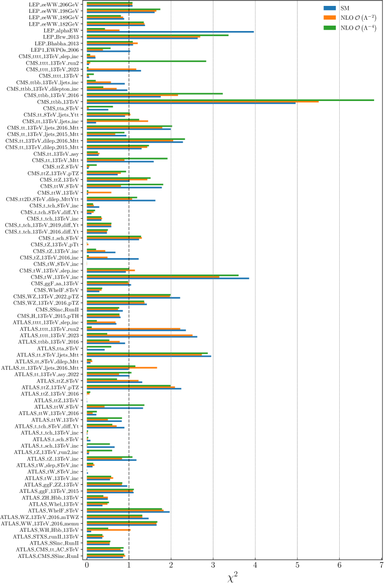
Figure 3.1: The values of the $\chi^{2}/n_{\rm dat}$ for the datasets entering the SMEFiT3.0 analysis. We compare the results based on the SM prediction with the outcome of the SMEFT fits, both at linear and quadratic order in the EFT expansion. See also Table 3.3 for the corresponding results grouped in terms of physical processes.

Dataset	$n_{\rm dat}$	$\chi^{2}_{\rm SM}/n_{\rm dat}$	$\chi^{2}_{\rm EFT}/n_{\rm dat}$	$\chi^{2}_{\rm EFT}/n_{\rm dat}$
			$\mathcal{O}\left(\Lambda^{-2}\right)$	$\mathcal{O}\left(\Lambda^{-4}\right)$
$t\bar{t}$ inclusive	115	1.365	1.193	1.386
$t\bar{t}+\gamma$	2	0.465	0.027	0.598
$t\bar{t}+V$	21	1.200	1.100	1.165
single-top inclusive	28	0.439	0.393	0.407
single-top $+V$	13	0.663	0.540	0.562
$t\bar{t}b\bar{b}$ & $t\bar{t}t\bar{t}$	12	1.396	1.386	1.261
Higgs production & decay	129	0.687	0.692	0.676
Diboson (LEP+LHC)	81	1.481	1.429	1.436
LEP + SLD	44	1.237	0.942	1.002
Total	445	1.087	0.992	1.048

Table 3.3: Summary of the $\chi^{2}/n_{\rm dat}$ results displayed in Fig. 3.1 in terms of the groups of processes entering the fit.

The $\chi^{2}$ values collected in Fig. 3.1 and Table 3.3 indicate that, for most of the datasets considered here, the SM predictions are in good agreement with the experimental data. This agreement remains the same, or it is further improved, at the level of the (linear or quadratic) EFT fits. However, for some datasets, the SM $\chi^{2}$ turns out to be poor. In most cases, this happens for datasets containing one or a few cross-section points. Datasets with a poor $\chi^{2}$ to the SM include CMS_ttbb_13TeV, CMS_tW_13TeV inc, ATLAS_tttt 13TeV_2023, ATLAS_tt_8TeV_ljets_Mtt, and ATLAS_ttZ_13TeV_pTZ. For these datasets, a counterpart from the complementary experiment is also part of the fit and agreement with the SM is found there, suggesting some tension between the ATLAS and CMS measurements. See also the discussions in Kassabov:2023hbm for the top quark datasets at the light of the covariance matrix decorrelation method Kassabov:2022pps . This interpretation is supported by the fact that, for these datasets with a poor $\chi^{2}$ to the SM prediction, accounting for EFT effects does not improve the agreement with the data. In such cases, the poor $\chi^{2}$ values may be explained by either internal inconsistencies Kassabov:2022pps or originates from tensions between different measurements of the same process.

Concerning the LEP measurements, good agreement with the SM is observed with the only exception of the electroweak coupling constant $\alpha_{\rm EW}$ and the $W$ branching ratios. While the $\chi^{2}$ to the former observable improves markedly once EFT corrections are accounted for, the opposite appears to be true for the LEP $W$-boson branching ratios. We recall here that, for the $W$ branching fractions in Eq. (2.37), possible invisible decay channels are not accounted for.

In Table 3.3, we present the $\chi^{2}$ values grouped by physical process, comparing the SM with the best fit parameters found in the SMEFT fits. Notably, the SM demonstrates a commendable per data point $\chi^{2}=1.087$, a value that further refines to 0.992 and 1.048 for the linear and quadratic EFT fits, respectively, with $n_{\text{eft}}=45$ and 50 parameters in each case. While the $\chi^{2}$ values of the Higgs production and decay dataset are similar in the SM and in the linear and quadratic EFT fits, and likewise for diboson production, more variation is found for the top-quark production datasets, specially for inclusive $t\bar{t}$ production. In the case of the EWPOs, there is a clear reduction of the $\chi^{2}$ per data point in the EFT fit as compared to the baseline SM predictions. It is worth emphasizing that these $\chi^{2}$ values do not imply that the EFT model offers a superior description to the data. Indeed, a thorough hypothesis test mandates normalizing the $\chi^{2}$ by the number of degrees of freedom $n_{\text{dof}}=n_{\text{dat}}-n_{\text{eft}}$. In this sense, the SM, having a good $\chi^{2}$ with less parametric freedom, remains the preferred model to describe the available data.

Constraints on the EFT operators.

Fig. 3.2 displays the results of SMEFiT3.0 at the level of the $n_{\rm eft}=45~{}(50)$ operators entering the analysis at the linear (quadratic) EFT level. The right panel shows the best-fit values and the 68% and 95% CL intervals, both for the linear and for the quadratic baseline fits. The reported bounds are extracted from a global fit with all coefficients being varied simultaneously, and then the resultant posterior distributions are marginalised down to individual coefficients. From top to bottom, we display the four-heavy quark, two-light-two-heavy quark, two-fermion, four-lepton, and purely bosonic coefficients. The corresponding information on the magnitude of the 95% confidence interval is provided in the left panel of Fig. 3.2.

The bounds displayed in Fig. 3.2 are also collected in Table 3.4, where for completeness we also include the individual bounds obtained from one parameter fits to the data (with all other coefficients set to zero). It is worth noting that for some operators at the quadratic EFT level the 95% CL bounds are disjoint, indicating the presence of degenerate solutions. For the four-heavy operators, in the linear fit one can only display the individual bounds, since in this sector the SMEFT displays flat directions (for the available data) unless quadratic corrections are included.

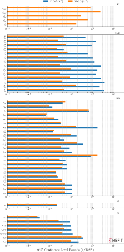
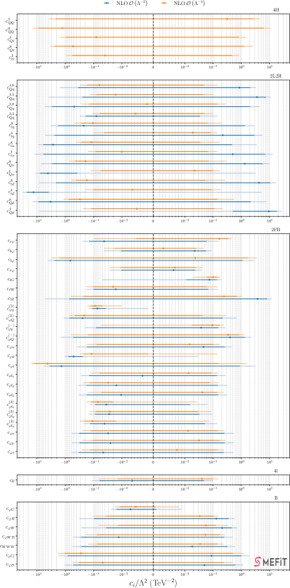
Figure 3.2: Left: The length of the 95% confidence bounds, expressed in units of 1/TeV^-2, for the $n_{\rm eft}=50$ coefficients entering the fit, both for linear and for quadratic (marginalised) analyses. From top to bottom we display the two-fermion, two-light-two-heavy quark, four-heavy quark (except for the linear fit), and the purely bosonic coefficients. Right: the coefficients $c_{i}/\Lambda^{-2}$ for the same fits, where the thicker (thinner) line indicates the 68% CL (95% CL) uncertainties. The vertical dashed line indicates the SM expectation for the values of these coefficients.

Class	DoF	95% CL bounds, $\mathcal{O}\left(\Lambda^{-2}\right)$		95% CL bounds, $\mathcal{O}\left(\Lambda^{-4}\right)$,
		Individual	Marginalised	Individual	Marginalised
4H	$c_{QQ}^{1}$	[1.648, 24.513]	—	[-2.403, 2.153]	[-3.765, 4.487]
	$c_{QQ}^{8}$	[3.343, 63.182]	—	[-7.196, 6.533]	[-13.586, 10.491]
	$c_{Qt}^{1}$	[-509.511, 211.968]	—	[-1.945, 1.958]	[-1.546, 1.455]
	$c_{Qt}^{8}$	[1.632, 21.393]	—	[-4.415, 3.607]	[-3.500, 2.549]
	$c_{tt}^{1}$	[0.768, 12.075]	—	[-1.201, 1.070]	[-0.919, 0.836]
2L2H	$c_{Qq}^{1,8}$	[-0.363, 0.201]	[-1.547, 3.207]	[-0.292, 0.141]	[-0.296, 0.144]
	$c_{Qq}^{1,1}$	[-1.154, 0.096]	[-3.820, 11.011]	[-0.150, 0.096]	[-0.136, 0.105]
	$c_{Qq}^{3,8}$	[-1.285, 0.417]	[-5.313, 4.288]	[-0.355, 0.229]	[-0.278, 0.282]
	$c_{Qq}^{3,1}$	[-0.128, 0.106]	[-0.301, 0.141]	[-0.092, 0.080]	[-0.112, 0.097]
	$c_{tq}^{8}$	[-0.639, 0.236]	[-3.270, 2.885]	[-0.459, 0.180]	[-0.467, 0.208]
	$c_{tq}^{1}$	[0.176, 1.188]	[-5.092, 5.481]	[-0.073, 0.160]	[-0.104, 0.139]
	$c_{tu}^{8}$	[-0.675, 0.247]	[-8.866, 3.490]	[-0.439, 0.179]	[-0.422, 0.175]
	$c_{tu}^{1}$	[-1.622, 0.214]	[-12.084, 12.836]	[-0.178, 0.126]	[-0.159, 0.139]
	$c_{Qu}^{8}$	[-1.567, 0.076]	[-7.200, 9.684]	[-0.702, 0.211]	[-0.715, 0.289]
	$c_{Qu}^{1}$	[0.210, 1.596]	[-11.379, 3.183]	[-0.101, 0.193]	[-0.129, 0.171]
	$c_{td}^{8}$	[-1.677, 0.206]	[-8.511, 16.583]	[-0.685, 0.244]	[-0.603, 0.266]
	$c_{td}^{1}$	[-3.955, -0.251]	[-31.597, 5.147]	[-0.234, 0.172]	[-0.198, 0.186]
	$c_{Qd}^{8}$	[-3.147, -0.091]	[-13.997, 7.530]	[-1.108, 0.326]	[-1.158, 0.549]
	$c_{Qd}^{1}$	[0.840, 3.755]	[-8.140, 26.827]	[-0.149, 0.242]	[-0.230, 0.216]
2FB	$c_{c\varphi}$	[-0.022, 0.120]	[-0.243, 0.154]	[-0.000, 0.373]	[-0.094, 0.442]
	$c_{b\varphi}$	[-0.007, 0.040]	[-0.043, 0.088]	[-0.008, 0.036]	[-0.043, 0.046]
	$c_{t\varphi}$	[-1.199, 0.327]	[-4.142, 2.831]	[-1.168, 0.333]	[-3.035, 3.527]
	$c_{\tau\varphi}$	[-0.027, 0.036]	[-0.027, 0.040]	[-0.024, 0.041]	[-0.027, 0.043]
	$c_{tG}$	[0.004, 0.084]	[-0.050, 0.199]	[0.003, 0.080]	[0.019, 0.180]
	$c_{tW}$	[-0.087, 0.029]	[-0.180, 0.147]	[-0.082, 0.029]	[-0.177, 0.141]
	$c_{tZ}$	[-0.034, 0.102]	[-4.999, 12.276]	[-0.038, 0.094]	[-0.645, 1.027]
	$c_{\varphi q}^{(3)}$	[-0.015, 0.012]	[-0.147, -0.002]	[-0.015, 0.012]	[-0.166, -0.010]
	$c_{\varphi Q}^{(3)}$	[-0.016, 0.023]	[-1.155, 0.665]	[-0.016, 0.023]	[-0.685, 0.271]
	$c_{\varphi q}^{(-)}$	[-0.121, 0.119]	[-0.193, 0.269]	[-0.118, 0.119]	[-0.056, 0.239]
	$c_{\varphi Q}^{(-)}$	[-0.031, 0.046]	[-1.427, 2.224]	[-0.031, 0.047]	[-0.620, 1.292]
	$c_{\varphi u}$	[-0.071, 0.081]	[-0.375, 0.461]	[-0.077, 0.079]	[-0.168, 0.177]
	$c_{\varphi d}$	[-0.140, 0.071]	[-1.038, 0.030]	[-0.137, 0.072]	[-0.303, 0.143]
	$c_{\varphi t}$	[-2.855, 1.036]	[-5.750, 3.084]	[-4.000, 0.872]	[-15.638, 1.532]
	$c_{\varphi l_{1}}$	[-0.009, 0.012]	[-0.276, 0.273]	[-0.008, 0.012]	[-0.133, 0.150]
	$c_{\varphi l_{2}}$	[-0.031, 0.017]	[-0.334, 0.302]	[-0.030, 0.017]	[-0.237, 0.166]
	$c_{\varphi l_{3}}$	[-0.035, 0.025]	[-0.329, 0.311]	[-0.034, 0.025]	[-0.150, 0.231]
	$c_{\varphi l_{1}}^{(3)}$	[-0.015, 0.009]	[-0.136, 0.064]	[-0.015, 0.009]	[-0.170, 0.027]
	$c_{\varphi l_{2}}^{(3)}$	[-0.031, 0.002]	[-0.146, 0.089]	[-0.031, 0.002]	[-0.137, 0.085]
	$c_{\varphi l_{3}}^{(3)}$	[-0.039, 0.017]	[-0.225, 0.141]	[-0.039, 0.017]	[-0.298, 0.073]
	$c_{\varphi e}$	[-0.025, 0.001]	[-0.583, 0.527]	[-0.025, 0.001]	[-0.254, 0.248]
	$c_{\varphi\mu}$	[-0.021, 0.039]	[-0.582, 0.533]	[-0.021, 0.038]	[-0.245, 0.277]
	$c_{\varphi\tau}$	[-0.045, 0.024]	[-0.597, 0.512]	[-0.045, 0.024]	[-0.261, 0.248]
4l	$c_{ll}$	[-0.008, 0.037]	[-0.112, 0.100]	[-0.008, 0.037]	[-0.066, 0.149]
B	$c_{\varphi G}$	[-0.001, 0.005]	[-0.024, 0.009]	[-0.002, 0.005]	[-0.018, 0.008]
	$c_{\varphi B}$	[-0.005, 0.002]	[-0.310, 0.573]	[-0.005, 0.002] $\cup$ [0.085, 0.092]	[-0.103, 0.152]
	$c_{\varphi W}$	[-0.018, 0.006]	[-0.273, 0.707]	[-0.017, 0.006] $\cup$ [0.282, 0.305]	[-0.067, 0.338]
	$c_{\varphi WB}$	[-0.007, 0.003]	[-0.525, 0.504]	[-0.007, 0.003]	[-0.190, 0.263]
	$c_{WWW}$	[-0.479, 0.607]	[-0.565, 0.609]	[-0.155, 0.197]	[-0.156, 0.230]
	$c_{\varphi\Box}$	[-0.416, 1.193]	[-1.715, 1.879]	[-0.429, 1.141]	[-1.856, 1.199]
	$c_{\varphi D}$	[-0.027, -0.003]	[-1.063, 1.149]	[-0.027, -0.003]	[-0.513, 0.483]

Table 3.4: The 95% CL bounds on the EFT coefficients considered in this analysis. The reported bounds correspond to $\Lambda=1$ TeV and can thus be rescaled for any other value of $\Lambda$. We present results both for linear EFT fits, $\mathcal{O}\left(\Lambda^{-2}\right)$, and for quadratic EFT fits, $\mathcal{O}\left(\Lambda^{-4}\right)$. In each case, we indicate both individual bounds (from one-parameter fits) and marginalised bounds (from a simultaneous determination of the full set of $n_{\rm eft}$ coefficients).

To further quantify the agreement between the SMEFT fit results and the corresponding SM expectations, Fig. 3.3 displays the fit residuals defined as

$$P_{i}\equiv\frac{\left\langle c_{i}\right\rangle-c_{i}^{(\rm SM)}}{\left[c_{i}^{\rm min},c_{i}^{\rm max}\right]^{68\%~{}{\rm CL}}}\,,\qquad i=1,\ldots,n_{\rm eft}\,,$$ (3.1)

in the same format as that of Fig. 3.2 for both linear and quadratic fits. Given that $c_{i}^{(\rm SM)}=0$ and that Eq. (3.1) is normalised to the 68% CL intervals (which in linear fits correspond to the standard deviation $\sigma$), a residual larger than 2 (in absolute value) indicates a coefficient that does not agree with the SM at the 95% CL.

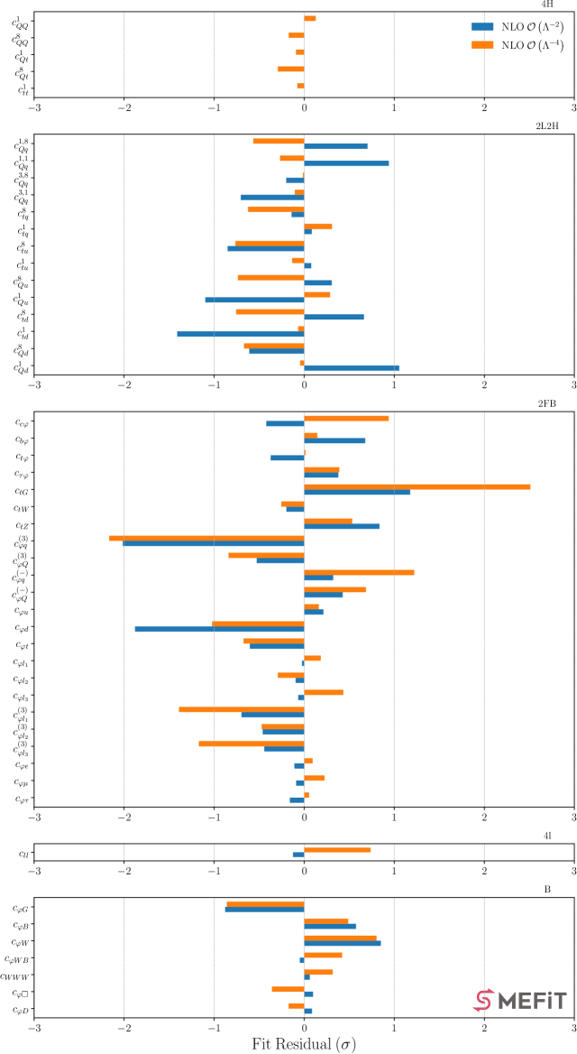
Figure 3.3: The residuals between the fit results and the SM expectations defined as in Eq. (3.1), for the operators entering Fig. 3.2 and for both linear and quadratic fits. These residuals are normalised to the 68% CL intervals, hence a residual larger than 2 (in absolute value) indicates a coefficient that disagrees with the SM at the 95% CL.

Several observations can be derived from the inspection of Figs. 3.2 and 3.3 as well as Table 3.4. First, the fit residuals evaluated in Fig. 3.3, consistently with Fig. 3.2, confirm that in general there is a good agreement between the EFT fit results and the experimental data. For the purely bosonic, four-lepton, four-heavy, and two-light-two-heavy operators, the fit residuals satisfy $|P_{i}|\mathrel{\hbox to0.0pt{\lower 4.0pt\hbox{\hskip 1.0pt$\sim$}\hss}\raise 1.0pt\hbox{$<$}}1$, the only exception being $c_{td}^{1}$ in the linear fit for which $P_{i}\sim 1.5$. Somewhat larger residuals are found for a subset of the two-fermion operators, in particular for the chromomagnetic operator coefficient $c_{tG}$ (only in the quadratic fit), for $c_{\varphi q}^{(3)}$, and for $c_{\varphi d}$ (only in the linear fit). For these coefficients, the values of $|P_{i}|$ range between 2 and 2.5. Below we investigate the origin of these large fit residuals.

One also finds that quadratic EFT corrections improve the bounds on most operators entering the fit, with a particularly marked impact for the two-light-two-heavy operators. The only exceptions of this trend are $c_{\varphi t}$, which is poorly constrained to begin with, and the charm Yukawa $c_{c\varphi}$. For both coefficients, the worse bounds arising in the quadratic fit are explained by the appearance of a second, degenerate solution, as demonstrated by the corresponding posterior distributions displayed in Fig. 3.7. Such degenerate solutions may arise Ethier:2021bye when quadratic corrections become comparable in magnitude with opposite sign to the linear EFT cross-section, a configuration formally equivalent to setting $c_{i}=0$ and hence reproducing the SM.

As is well known Hartland:2019bjb , quadratic EFT corrections also allow one to bound the four-heavy operator coefficients $c_{tt}^{1}$, $c_{Qt}^{1}$, $c_{Qt}^{8}$, $c_{QQ}^{1}$, and $c_{QQ}^{8}$. Within a $\mathcal{O}\left(\Lambda^{-2}\right)$ fit, only two linear combinations of these four-heavy operators can be instead constrained, leaving three flat directions. These considerations do not hold for one-parameter fits, where the four-heavy operators can be separately constrained. From Fig. 3.2, one can also see that for some operators the effects of the quadratic EFT corrections are essentially negligible, indicating that the linear (interference) cross-section dominates the sensitivity. Specifically, operators for which quadratic corrections are small are the four-lepton operator $c_{\ell\ell}$, the two-fermion operators $c_{\varphi q}^{3}$, $c_{\varphi\ell_{i}}^{3}$ (with $i=1,\,2,\,3$), $c_{tW}$, and the tau and top Yukawa couplings, $c_{\tau\varphi}$ and $c_{t\varphi}$ respectively.

The comparison between global (marginalised) and individual (one-parameter) fit results reported in Table 3.4 indicates that, for the linear EFT fits, one-parameter bounds are always tighter than the marginalised ones. The differences between individual and marginalised bounds span a wide range of variation, from $c_{WWW}$, which essentially shows no difference, to $c_{\varphi D}$, with individual bounds tighter by two orders of magnitude as compared to the marginalised counterparts. Concerning the quadratic EFT fits, for the purely bosonic and two-fermion operators the situation is similar as in the linear case, with individual bounds either (much) tighter than the marginalised ones or essentially unchanged (as is the case for $c_{WWW}$ and $c_{\tau\varphi}$, for example). The situation is somewhat different for the four-heavy and two-light-two-heavy operators. For the latter, the marginalised and individual bounds are now similar to each other, as opposed to the linear fit case. For the four-heavy operators, the marginalised bounds are either similar or a bit broader than the individual ones, except in the case of $c_{Qt}^{(8)}$, whose 95% CL bounds $[-4.4,3.6]$ (individual) improve to $[-3.5,2.5]$ (marginalised), hence by a factor of approximately 30%. In such cases the correlations with other parameters entering the global fit improve the overall sensitivity compared to the one-parameter fits.

When interpreting the bounds on the EFT coefficients and the associated residuals displayed in Figs. 3.2 and 3.3, one should recall that in general there are potentially large correlations between them. To illustrate these, Fig. 3.4 (3.5) displays the entries of the correlation matrix, $\rho_{ij}$, for the $n_{\rm eff}=45$ (50) coefficients associated to the linear (quadratic) SMEFiT3.0 baseline analysis. To facilitate visualisation, entries with $|\rho_{ij}|<0.2$ (negligible correlations) are not shown in the plot.

The most noticeable feature comparing Figs. 3.4 and 3.5 is the fact that correlations become significantly weaker in the quadratic fit, especially for the two-light-two-heavy top quark operators as already noticed in Hartland:2019bjb , but also for some purely bosonic and two-fermion operators. Nevertheless, some large correlations remain also in the quadratic fit, and for instance $c_{\varphi D}$ is strongly anti-correlated with most of the operators constrained by the EWPOs. We recall that the correlation patterns in Figs. 3.4 and 3.5 depend on the specific fitted dataset, and in particular these patterns change qualitatively once we include the FCC-ee projections in Sect. 4.

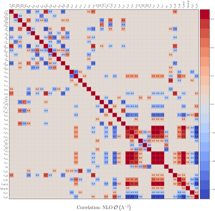
Figure 3.4: The correlation matrix for the $n_{\rm eff}=45$ coefficients associated to the linear SMEFiT3.0 baseline analysis. To facilitate visualisation, the EFT coefficients whose correlation with all other coefficients is $<0.2$ are removed from the plot.

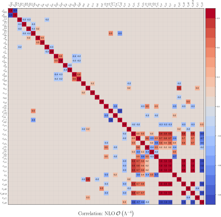
Figure 3.5: Same as Fig. 3.4, now for the SMEFiT3.0 baseline analysis carried out with $\mathcal{O}\left(\Lambda^{-4}\right)$ corrections.

Coefficients with large residuals.

As mentioned above, the fit residual analysis of Fig. 3.3 indicates that three Wilson coefficients, namely $c_{tG}$ (in the quadratic fit), $c_{\varphi d}$ (in the linear fit), and $c_{\varphi q}^{3}$ (in both cases) do not agree with the SM expectation at the 95% CL, with pulls of $P_{i}\simeq+2.5,-1.9$, and $-2.1$ respectively. The corresponding individual (one-parameter) analysis of Table 3.4 indicates that for these coefficients the pulls are $P_{i}\simeq+2.0,-0.3$, and $-0.2$ respectively, when fitted setting all other operators to zero. Therefore, the pull on $c_{tG}$ in the quadratic case is somewhat reduced in individual fits but does not go away, while the large pulls on $c_{\varphi q}^{3}$ and $c_{\varphi d}$ completely disappear in the one-parameter fits. The latter result indicates that the pulls of $c_{\varphi q}^{3}$ and $c_{\varphi d}$ found in the global fit arise as a consequence of the correlations with other fit parameters.

In the case of the chromomagnetic operator coefficient $c_{tG}$, the tension with the SM which arises in the quadratic fit was already present in previous versions of our analysis Ethier:2021bye ; Giani:2023gfq and is known to be driven by the CMS top-quark double-differential distributions in $(y_{t\bar{t}},m_{t\bar{t}})$ at $8$ TeV from CMS:2017iqf . In the context of a linear EFT fit, the obtained residual is consistent with the SM, a finding also in agreement with the independent analysis carried out in Kassabov:2023hbm . Indeed, if this CMS double-differential $t\bar{t}$ 8 TeV measurement is excluded from the quadratic fit, $c_{tG}$ becomes fully consistent with the SM expectation. We also note that this dataset, with $\chi^{2}_{\rm SM}/n_{\rm dat}\simeq 1.7$ for $n_{\rm dat}=16$ points, improves down to $\chi^{2}_{\rm EFT}/n_{\rm dat}\simeq 1$ after the fit. Given that $c_{tG}$ modifies the overall normalisation of top-quark pair production, rather than the shape of the distributions, this result may imply that the normalisation of this 2D CMS measurement is in tension with that of other $t\bar{t}$ measurements included in the fit. All in all, it appears unlikely that this large pull on $c_{tG}$ obtained in the quadratic fit is related to a genuine BSM signal.

Regarding the $c_{\varphi d}$ and $c_{\varphi q}^{(3)}$ Wilson coefficients, we note pulls of approximately $-1.9$ and $-2.1$, respectively, in the linear fit. However, in the quadratic fit, the pull for $c_{\varphi d}$ decreases to around $-1.0$. Notably, the individual constraints are instead entirely consistent with the SM. This pattern arises from the predominance of LEP data in individual fits, where no deviations from the SM are apparent. However, in a comprehensive global fit, the LEP data exhibit strong inter-coefficient correlations, leading to a notable reduction in their constraining effectiveness. As is well-established, the complementary nature of LHC diboson measurements to EWPO is crucial to break several of these correlations. For this reason, the LHC diboson data, despite being less precise, can have a surprising impact on the bounds of the EFT coefficients affecting LEP observables. We have confirmed that these measurements are indeed responsible for the observed pulls in the global fit.

Exact versus approximate implementation of the EWPOs.

Fig. 3.6 displays a comparison at the level of the posterior distributions on the Wilson coefficients between the new implementation of the EWPOs presented in Sect. 2 and used in SMEFiT3.0 and the previous, approximate implementation entering SMEFiT2.0 and based on imposing the restrictions in Eq. (2.31). In both cases, these posteriors correspond to global marginalised fits carried out at $\mathcal{O}\left(\Lambda^{-4}\right)$ in the EFT expansion, see also Table A.1.

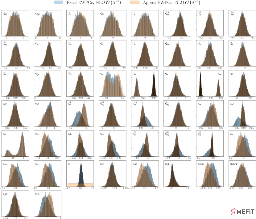
Figure 3.6: Posterior distributions associated to the $n_{\rm eft}=50$ Wilson coefficients constrained in the SMEFiT3.0 global analysis, carried out at $\mathcal{O}\left(\Lambda^{-4}\right)$ in the EFT expansion. A simultaneous determination of all coefficients is performed and then one marginalises for individual degrees of freedom. The baseline results, performed with the exact implementation of the EWPOs, are compared with the approximated implementation used in Ethier:2021bye .

From this comparison one observes that the exact implementation of the EWPOs does not lead to major qualitative differences in the posterior distributions. Nevertheless, the approximate implementation of the EWPOs was in some cases too aggressive, and when replaced by the exact implementation one observes how the associated posterior distributions may display a broadening, as is the case for instance for the $c_{\varphi\ell_{3}}^{(3)}$ and $c_{\varphi d}$ coefficients. Other EFT degrees of freedom for which the posterior distributions are modified following the exact implementation of the EWPOs are $c_{\varphi\ell_{3}},\,c_{\varphi\ell_{2}}^{(3)},\,c_{\varphi q}^{(3)},\,c_{\varphi q}^{(-)},\,$ and $c_{\ell\ell}$. In particular, we note that the four-lepton coefficient $c_{\ell\ell}$ was set to zero in the approximate implementation, while now it enters as an independent degree of freedom.

Two-light-two-heavy and four-heavy operators are constrained mostly by a set of processes not sensitive to the operators entering the EWPOs, i.e. top pair production and four-heavy quark production. There is limited cross-talk between the four-heavy operators and those entering the EWPOs, and hence the posteriors of the former remain unchanged comparing the two fits. Furthermore, for other operators which are not directly sensitive to the EWPOs, we have verified that the residual observed differences arise from their correlations within the global fit with coefficients modifying the electroweak sector of the SMEFT (and they are hence absent in one-parameter individual fits), see also Figs. 3.4 and 3.5.

We conclude from this analysis that, at the level of sensitivity that global SMEFT fits such as the one presented in this work are achieving, it is crucial to properly account for the constraints provided by the precise EWPOs from electron-positron colliders.

Impact of new LHC Run II data.

Next we quantify the impact of the new LHC Run II measurements included in the analysis, in comparison with SMEFiT2.0, and listed in Sect. 3.1. To this end, we compare the baseline global SMEFT fit with a variant in which the input dataset is reduced to match that used in our previous analyses Ethier:2021bye ; Giani:2023gfq . In both cases, methodological settings and theory calculations are kept identical, and in particular both fits include the exact implementation of the EWPOs, quadratic EFT effects, and NLO QCD corrections to the EFT cross-sections, see also Table A.1. Hence the only difference between the two results concerns the LHC Run II data being fitted.

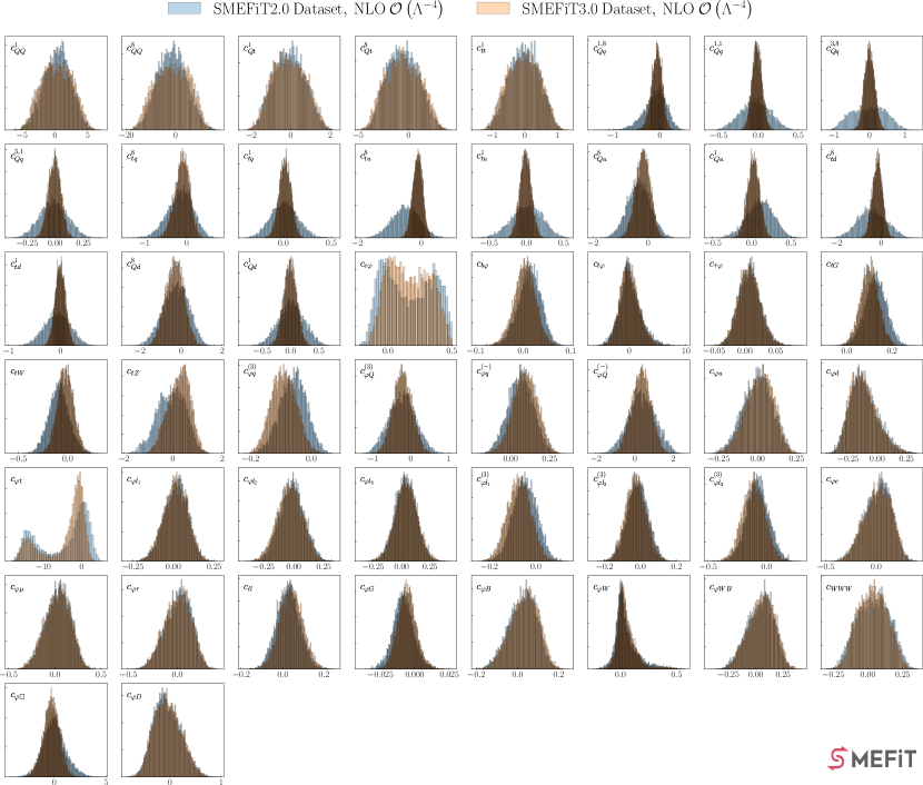
Figure 3.7: Same as Fig. 3.6 now comparing the results of the global analysis based on the SMEFiT2.0 and SMEFiT3.0 datasets, all other settings and theory calculations kept the same. In particular, in both cases the baseline settings includes the exact implementation of the EWPOs.

Fig. 3.7 displays the same comparison of the results of the global analysis based on the SMEFiT2.0 and SMEFiT3.0 datasets. The most marked impact of the new data is observed for the two-light-two-heavy four-fermion operators, where the narrower posterior distributions reflect improved bounds by a factor between 2 and 3 compared to the fit to the SMEFiT2.0 dataset, depending on the specific operator. In all cases, the posterior distributions for the two-light-two-heavy operators remain consistent with the SM expectation at the 68% CL interval, see also Fig. 3.3.

Other coefficients for which the new data brings in moderate improvements include the charm Yukawa $c_{c\varphi}$ (thanks to the latest Run II measurements which constrain the Higgs branching ratios and hence the total Higgs width), $c_{tZ}$ and $c_{\varphi t}$ (from the new $t\bar{t}Z$ dataset). For the other coefficients, the impact of the new datasets is minor. In particular, the latest measurements on $t\bar{t}t\bar{t}$ and $t\bar{t}b\bar{b}$ leave the posterior distributions of the four-heavy-fermion operators essentially unchanged.

Furthermore, one notes that the bound on the triple-gauge coupling operator $\mathcal{O}_{WWW}$ does not improve upon the inclusion of diboson production measurements based on the full Run II luminosity. However, we should emphasise that including diboson production in proton-proton collisions in the fit plays an important role in breaking flat directions from EWPOs, for example in the $\left(c_{\varphi q}^{(3)},c_{\varphi q}^{(-)}\right)$ plane. As we will also see in Sect. 3.3, (HL)-LHC diboson measurements are crucial in improving the bounds on various two-light-fermion coefficients.

3.3 Projections for the HL-LHC

We now assess the impact of projected HL-LHC measurements when added on top of the SMEFiT3.0 baseline fit. These projections are constructed following the procedure described in App. D, where we also list the processes considered. In a nutshell, we take existing Run II measurements for a given process, focusing on datasets obtained from the highest luminosity, and extrapolate their statistical and systematic uncertainties to the HL-LHC data-taking period. Specifically, the statistical uncertainties in the projected pseudo-data are reduced by a factor depending on the ratio of luminosities, while systematic uncertainties are reduced by a fixed factor (taken to be 1/2 in our case) based on the expected performance improvement of the detectors.

Within the adopted procedure, we maintain the settings and binning of the original Run II analysis unchanged, and assume the SM as the underlying theory. We note that our projections are not optimised, and in particular with a higher luminosity one could also extend the kinematic coverage of the high-$p_{T}$ regions Durieux:2022cvf , adopt a finer binning, or attempt multi-differential measurements. Nevertheless, our approach benefits from being exhaustive and systematic, and is also readily extendable once new Run II and III measurements become available.

Since the considered HL-LHC projections assume the SM as the underlying theoretical description, and to avoid introducing possible inconsistencies, we generate Level-1 SM pseudo-data for the full SMEFiT3.0 dataset and use it to produce a baseline fit for the subsequent inclusions of the HL-LHC pseudo-data, see also Table A.1. In Level-1, the pseudo-data is fluctuated randomly within uncertainties around the central SM theoretical prediction (see App. D). This is the same strategy adopted in the closure tests entering the NNPDF proton structure analyses NNPDF:2014otw ; NNPDF:2021njg . A dataset consistent with the SM as underlying theory throughout enables to cleanly separate the sensitivity of the projected data to the SMEFT parameter space from other possible factors, such as dataset inconsistency, eventual BSM signals, or the interplay with QCD uncertainties such as those associated to the PDFs. We have verified that, in the SMEFT analyses based on pseudo-data generated this way, the fit quality satisfies $\chi^{2}/n_{\rm dat}\sim 1$ as expected (see Fig. D.1), both for the baseline fit and once the HL-LHC (and later the FCC-ee and CEPC) projections are included. For this reason, in the following we only present results for the relative reduction of the uncertainties associated to the Wilson coefficients, since the central values are by construction consistent with the SM expectations.

In the rest of this section and in the following one, we present results in terms of $R_{\delta c_{i}}$, defined as the ratio between the magnitude of the 95% CL interval for a given EFT coefficient $c_{i}$, to that of the same quantity in the baseline fit:

$$R_{\delta c_{i}}=\frac{\left[c_{i}^{\rm min},c_{i}^{\rm max}\right]^{95\%~{}{\rm CL}}~{}({\rm baseline+\text{HL-LHC}})}{\left[c_{i}^{\rm min},c_{i}^{\rm max}\right]^{95\%~{}{\rm CL}}~{}({\rm baseline})}\,,\qquad i=1,\ldots,n_{\rm eft}\,.$$ (3.2)

In the case of a disjoint 95% CL interval, we add up the magnitudes of the separate regions. From the definition of Eq. (3.2) it is clear that, for a given coefficient $c_{i}$, the smaller the value of $R_{\delta c_{i}}$ the more significant the impact of the new data.

As mentioned above, central values are by construction in agreement with the SM expectation ($c_{i}^{\rm(SM)}=0$) within uncertainties, and hence it is not necessary to display them in these comparisons. The ratio Eq. (3.2) can be evaluated both in one-parameter fits as well as in the global fit followed by marginalisation. In contrast with Level-1 pseudo-data, Level-0 pseudo-data has central values identical to the SM predictions, and do not account for statistical fluctuations in the experimental measurements; for completeness, we also display Level-0 projection results in App. D.

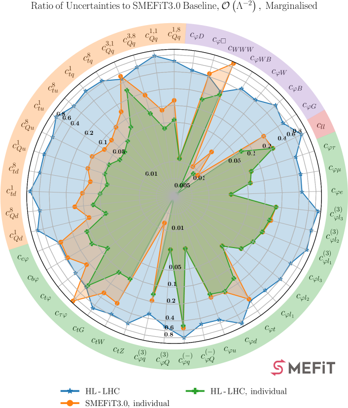
Figure 3.8: The ratio of uncertainties $R_{\delta c_{i}}$, defined in Eq. (3.2), for the $n_{\rm eft}=45$ coefficients entering the linear EFT fit, quantifying the impact of the HL-LHC projections when added on top of the SMEFiT3.0 baseline. We display both the results of one-parameter fits and those of the marginalised analysis. The different color codes indicate the relevant groups of SMEFT operators: two-light-two-heavy operators (orange), two-fermion operators (green), purely bosonic operators (purple), and the four-lepton operator $c_{\ell\ell}$ (red). Note that here the baseline is a fit to pseudo-data for the SMEFiT3.0 dataset generated assuming the SM, rather than the fit to real data, see also Table A.1.

Fig. 3.8 displays the ratio of uncertainties $R_{\delta c_{i}}$, Eq. (3.2), for the $n_{\rm eft}=45$ Wilson coefficients entering the linear EFT fit, quantifying the impact of the HL-LHC projections when added on top of the SMEFiT3.0 baseline. We display both the results of the global fit, as well as those of one-parameter fits where all other coefficients are set to zero. Whenever available, as in the rest of this work, NLO QCD corrections for the EFT cross-sections are accounted for. Then in Fig. 3.9 we show the same comparison now in the case of the analysis with quadratic EFT corrections included in the theory calculations.

To facilitate visualisation, in Figs. 3.8 and 3.9 results are presented with a “spider plot” format, with the different colours on the perimeter indicating the relevant groups of SMEFT operators: two-light-two-heavy four-fermion operators, two-fermion operators, purely bosonic operators, four-heavy four-fermion operators, and the four-lepton operator $c_{\ell\ell}$. Recall that the four-heavy operators, constrained by $t\bar{t}t\bar{t}$ and $t\bar{t}b\bar{b}$ production data, are excluded from the linear fit due to its lack of sensitivity. In this plotting format, coefficients whose values for $R_{\delta c_{i}}$ are closer to the center of the plot correspond to the operators which are the most constrained by the HL-LHC projections, in the sense of the largest reduction of the corresponding uncertainties. These plots adopt a logarithmic scale for the radial coordinate, to better highlight the large variations between the $R_{\delta c_{i}}$ values obtained for the different coefficients.

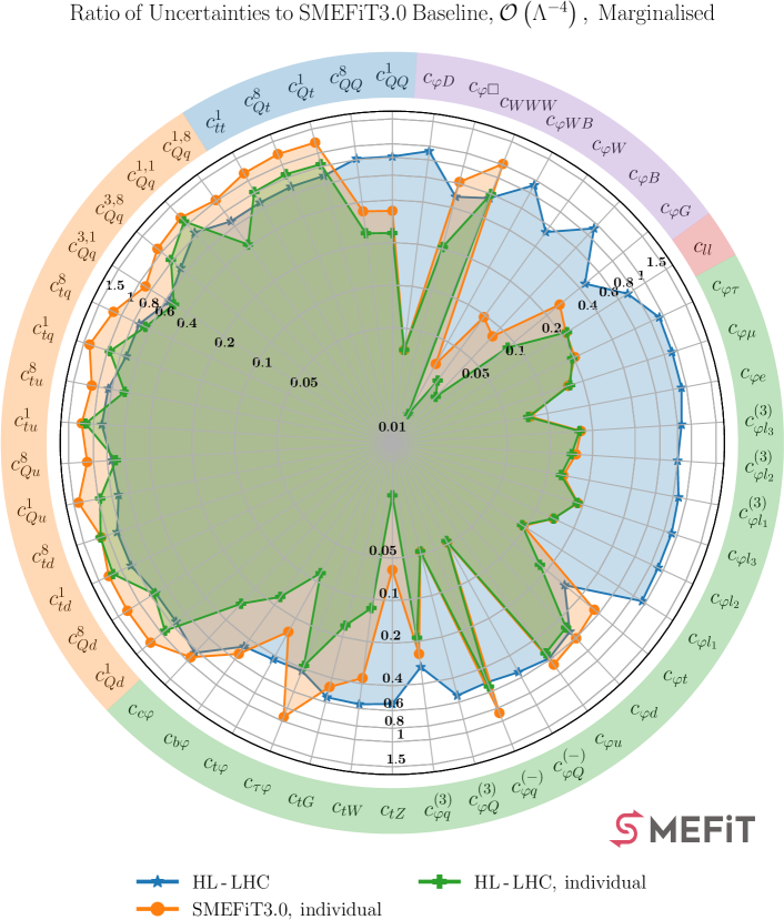
Figure 3.9: Same as Fig. 3.8, now in the case of the analysis with quadratic EFT corrections included. Note that in comparison with the linear fits, we now have an extra group of operators (indicated in blue), namely the four-heavy four-fermion operators that are constrained by $t\bar{t}t\bar{t}$ and $t\bar{t}b\bar{b}$ production data.

Several observations are worth drawing from the results of Figs. 3.8 and 3.9. Considering first the linear EFT fits, one observes that the projected HL-LHC observables are expected to improve the precision in the determination of the considered Wilson coefficients by an amount which ranges between around 20% and a factor 3, depending on the specific operator, in the global marginalised fits. For instance, we find values of $R_{\delta c_{i}}\simeq 0.3$ for the triple gauge coupling $c_{WWW}$ and of $R_{\delta c_{i}}\simeq 0.4$ for the charm, bottom, and tau Yukawa couplings $c_{b\varphi}$, $c_{c\varphi}$, and $c_{\tau\varphi}$. For the two-light-two-heavy operators bounds, driven by $t\bar{t}$ distributions, $R_{\delta c_{i}}$ ranges between 0.8 and 0.5 hence representing up to a factor two of improvement. For the operators driven by top quark production, our estimate of the impact of the HL-LHC data can be compared to the results of deBlas:2022ofj ; Durieux:2022cvf . Their analysis includes dedicated HL-LHC observables which especially help for the two-light-two-heavy operators, resulting in tighter bounds as compared to our fit by around a factor two for some of these coefficients.

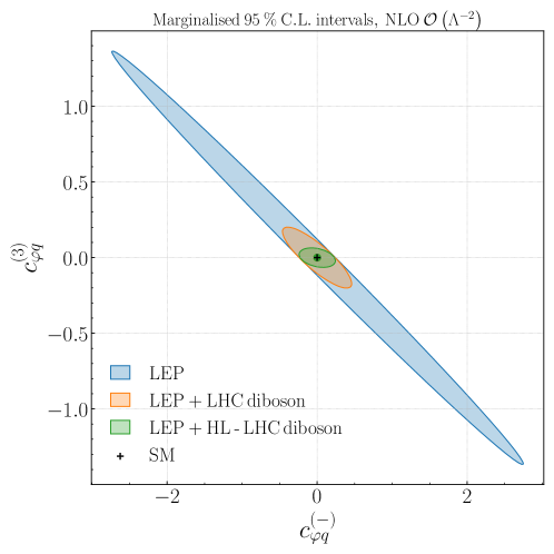
Figure 3.10: The $95\%$ CL marginalised intervals in the $\left(c_{\varphi q}^{(3)},c_{\varphi q}^{(-)}\right)$ plane from linear EFT fits to different datasets. We compare the result of a LEP-only fit (blue) with those adding either the LHC Run II diboson data (orange) or the HL-LHC diboson projections (green). The three fits are carried out with Level-0 pseudo-data, see App. D.

Additionally, HL-LHC measurements can improve the bounds imposed by EWPOs along directions that are a linear combination of individual coefficients, as illustrated by the $\left(c_{\varphi q}^{(3)},c_{\varphi q}^{(-)}\right)$ analysis of Fig. 3.10 where we show the impact of diboson production on the $95\%$ CL intervals in the $\left(c_{\varphi q}^{(3)},c_{\varphi q}^{(-)}\right)$ plane. We compare the marginalized bounds from a global linear LEP-only fit with those resulting from combining LEP with either LHC Run II or the HL-LHC diboson data. For consistency, the three fits are carried out with Level-0 pseudo-data. LEP data results in a quasi-flat direction in this plane, which is then well constrained by diboson data at LHC Run II (and subsequently at the HL-LHC), confirming the long-predicted complementarity between LEP and LHC diboson measurements Falkowski:2015jaa ; Butter:2016cvz ; Alioli:2017nzr ; Franceschini:2017xkh ; Banerjee:2018bio ; Grojean:2018dqj .

The broad reach of the HL-LHC program is illustrated by the fact that essentially all operators considered have associated tighter bounds even in the conservative analysis we perform. The comparison between the linear EFT marginalised and individual bounds displayed in Fig. 3.8 indicates that in the one-parameter fits the sensitivity is typically much better than in the global fit, in some cases by more than an order of magnitude, for example for the $c_{\varphi WB}$, $c_{\varphi B}$, $c_{\varphi W}$, and $c_{tZ}$ coefficients. The exception of this trend are coefficients which are determined by specific subsets of measurements which do not affect other degrees of freedom, such as $c_{WWW}$, constrained from diboson data, and $c_{\tau\varphi}$, constrained only from $h\to\tau\tau$ decays. This comparison between individual fits to the SMEFiT3.0 and HL-LHC datasets also highlights which operators are constrained mostly by the EWPOs, namely the two-light-fermion operators, the four-lepton operator $c_{\ell\ell}$, and the purely bosonic operator $c_{\varphi\square}$. For these coefficients, the improvements found in the global marginalised HL-LHC fit arise from indirect improvements in correlated coefficients.

Fig. 3.9 presents the same comparison as that in Fig. 3.8 now with the quadratic EFT corrections accounted for, and including also the results for the four-heavy four-fermion operators. Quadratic fits break degeneracies and correlations present in the linear fit. Hence, some operators not well probed at (HL-)LHC, such as the two-lepton ones, show an $R_{\delta c_{i}}$ closer to $1$ than in the linear case. Likewise, for these operators $R_{\delta c_{i}}$ is unchanged in the individual fits before and after the inclusion of the HL-LHC projections.

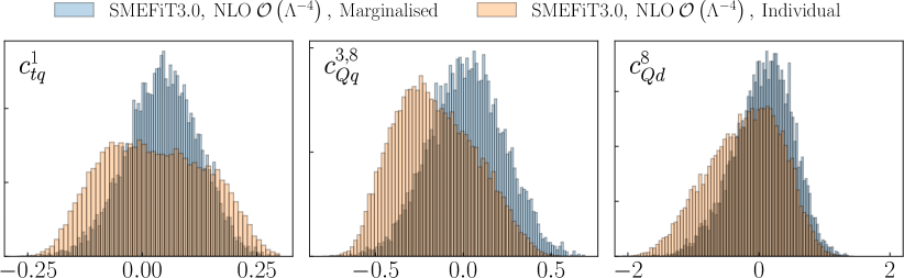
Figure 3.11: Posterior distributions for three operators which in the quadratic EFT analysis display looser individual (one-parameter) bounds in comparison with corresponding marginalised bounds. We show the two-light-two-heavy operators $c_{tq}^{1}$, $c_{Qq}^{3,8}$, and $c_{Qd}^{8}$. The two fits considered are based on the same global dataset.

A feature of Fig. 3.9 is that for some operators the individual bounds are looser than the marginalised ones, albeit by a moderate amount (up to 30%). This is the case for most of the two-light-two-heavy operators, and visible both with the SMEFiT3.0 dataset and for the fits with HL-LHC pseudo-data. To investigate the origin of this feature, Fig. 3.11 shows posterior distributions for three operators (the two-light-two-heavy operators $c_{tq}^{1}$, $c_{Qq}^{3,8}$, and $c_{Qd}^{8}$) which in the quadratic EFT analysis display looser individual bounds in comparison with corresponding marginalised bounds. For these operators, the marginalised fits lead to narrower posterior distributions, explaining the observed more stringent constraints. Finally, we note that in scenarios relevant to the matching to UV models, which involve a subset of EFT operators, the relevant constraints would be in between the global and the individual bounds shown in Fig. 3.9.

Overall, our analysis indicates that, in the context of a global SMEFT fit, the extrapolation of Run II measurements to the HL-LHC results into broadly improved bounds, ranging between 20% and a factor 3 better depending on the specific coefficient. Qualitatively similar improvements arising from HL-LHC constraints will be observed once matching to UV models in Sect. 5. We note again that the HL-LHC constraints derived here are conservative, as they may be significantly improved through optimised analyses, exploiting features not accessible with the Run II dataset.

4 The impact of future $e^{+}e^{-}$ colliders on the SMEFT

We now present the quantitative assessment of the constraints on the SMEFT coefficients provided by measurements to be carried out at the two proposed high-energy $e^{+}e^{-}$ circular colliders, FCC-ee and CEPC. The baseline for these projections is the global SMEFT analysis augmented with the dedicated HL-LHC projections from Sect. 3.3. Here first of all we describe the FCC-ee and CEPC observables and running scenarios considered, for which we follow the recent Snowmass study deBlas:2022ofj with minor modifications. Then we present results at the level of SMEFT coefficients, highlighting the correlation between LHC- and $e^{+}e^{-}$-driven constraints.

4.1 Observables and running scenarios

Several recent studies deBlas:2019rxi ; DeBlas:2019qco ; deBlas:2022ofj ; Durieux:2022cvf have assessed the physics potential of the various proposed leptonic colliders, including FCC-ee, ILC, CLIC, CEPC, and a muon collider, in terms of global fits to SMEFT coefficients and in some cases also matched to UV-complete models. Here we describe the projections for FCC-ee and CEPC measurements that will be used to constrain the SMEFT parameter space. We focus on these two colliders as representative examples of possible new leptonic colliders, though the same strategy can be straightforwardly applied to any other future facility.

The Future Circular Collider Benedikt:2020ejr ; FCC:2018byv in its electron-positron mode (FCC-ee) FCC:2018evy ; Bernardi:2022hny , originally known as TLEP TLEPDesignStudyWorkingGroup:2013myl , is a proposed electron-positron collider operating in a tunnel of approximately 90 km of circumference in the CERN site and based on well-established accelerator technologies similar to those of LEP. Running at several center-of-mass energies is envisaged, starting from the $Z$-pole all the way up to $\sqrt{s}=365$ GeV, above the top-quark pair production threshold. Possible additional runs at $\sqrt{s}=125$ GeV (Higgs pole) and for $\sqrt{s}<m_{Z}$ (for QCD studies) are under consideration for the FCC-ee. This circular $e^{+}e^{-}$ collider would represent the first stage of a decades-long scientific exploitation of the same tunnel, eventually followed by a $\sqrt{s}\sim 100$ TeV proton-proton collider (FCC-hh). Here we adopt the same scenarios for the FCC-ee running as in the Snowmass study of deBlas:2022ofj but updated to consider 4 interaction points (IPs), along the lines of the recent midterm feasibility report FCCfeasibility . We summarise the running scenarios in Table 4.1. As done in previous studies deBlas:2019rxi , we combine the information associated to the data taken at the runs with $\sqrt{s}=350$ GeV and $365$ GeV and denote this combination as “$\sqrt{s}=365$ GeV” in the following.

Energy $(\sqrt{s})$	$\mathcal{L}_{\rm int}$ (Run time)		$\mathcal{L}_{\rm FCC-ee}/\mathcal{L}_{\rm CEPC}$
	FCC-ee (4 IPs)	CEPC (2 IPs)
$91$ GeV ($Z$-pole)	$300$ ab-1 (4 years)	$100$ ab-1 (2 years)	3
$161$ GeV ($2\,m_{W}$)	$20$ ab-1 (2 years)	$6$ ab-1 (1 year)	3.3
$240$ GeV	$10$ ab-1 (3 years)	$20$ ab-1 (10 years)	0.5
$350$ GeV	$0.4$ ab-1 (1 year)	$0.2$ ab-1	2
$365$ GeV ($2\,m_{t}$)	$3$ ab-1 (4 years)	$1$ ab-1 (5 years)	3

Table 4.1: The running scenarios considered in our analysis for the FCC-ee and the CEPC, following deBlas:2022ofj ; Bernardi:2022hny ; CEPCPhysicsStudyGroup:2022uwl and the mid-term FCC feasibility report FCCfeasibility . Our projections assume 4 interaction points (IPs) for the FCC-ee and 2 for the CEPC. For each center of mass energy $\sqrt{s}$, we indicate the expected luminosity as well as the number of years in which this luminosity will be collected. The last column displays the ratio between the expected integrated luminosities at the FCC-ee and the CEPC. When presenting our results, we combine the information associated to the data taken at the runs with $\sqrt{s}=350$ GeV and $365$ GeV and denote this combination as “$\sqrt{s}=365$ GeV”.

The Circular Electron Positron Collider (CEPC) An:2018dwb is a proposed electron-positron collider to be built and operated in China. The current plan envisages a collider tunnel of around 100 km, and it would operate in stages at different center of mass energies, with a maximum of $\sqrt{s}=365$ GeV above the top-quark pair production threshold. The current baseline design assumes two interaction points for the CEPC. In the same manner as for the FCC-ee, Table 4.1 indicates the expected integrated luminosity (and number of years required to achieve it) in the current running scenarios for each value of the center-of-mass energy $\sqrt{s}$. The main differences between the projected statistical uncertainties for the FCC-ee and CEPC arise from the different data-taking plans as well as the different number of IPs. For instance, CEPC plans a longer running period at $\sqrt{s}=240$ GeV, which would lead to a reduction of statistical errors as compared to the FCC-ee observables corresponding to the same center-of-mass energy.

In the last column of Table 4.1 we display the ratio between the integrated luminosities at the FCC-ee and the CEPC, $\mathcal{L}_{\rm FCC-ee}/\mathcal{L}_{\rm CEPC}$, for each of the data-taking periods at a common center of mass energy. The FCC-ee is expected to accumulate a luminosity 3 times larger than the CEPC for the runs at $\sqrt{s}=91$ GeV, 161 GeV, and 365 GeV, while for $\sqrt{s}=240$ GeV it would accumulate half of the CEPC luminosity, given that the latter is planned to run for 10 years as opposed to the 3 years of the FCC-ee.

In our analysis, we consider five different classes of observables that are accessible at high-energy circular electron-positron colliders such as the FCC-ee and the CEPC. These are the EWPOs at the $Z$-pole; light fermion (up to $b$ quarks and $\tau$ leptons) pair production; Higgs boson production in both the $hZ$ and $h\nu\nu$ channels; gauge boson pair production; and top quark pair production. Diboson ($W^{+}W^{-}$) production becomes available at $\sqrt{s}=161$ GeV ($WW$ threshold), Higgs production opens up at $\sqrt{s}=240$ GeV, and top quark pair production is accessible starting from $\sqrt{s}=350$ GeV, above the $t\bar{t}$ threshold.

Among these processes, the $Z$-pole EWPOs, light fermion-pair, $W^{+}W^{-}$, and Higgs production data are included at the level of inclusive cross-sections, accounting also for the corresponding branching fractions. The complete list of observables considered, together with the projected experimental uncertainties entering the fit, are collected in App. E. For diboson and top quark pair production, we consider also unbinned normalised measurements within the optimal observables approach, described in App. F. We briefly review below these groups of processes.

EWPOs at the $Z$-pole.

The $Z$-pole electroweak precision observables that would be measured at the FCC-ee and CEPC coincide with those already measured by LEP and SLD and summarised in Table 2.1. The main difference is the greatly improved precision that will be achieved at future electron-positron colliders, due to the increased luminosity and the expected reduction of systematic uncertainties. Specifically, here we include projections for the QED coupling constant at the $Z$-pole, $\alpha(m_{Z})$; the decay widths of the $W$ and $Z$ bosons, $\Gamma_{W}$ and $\Gamma_{Z}$; the asymmetry between vector and axial couplings $A_{f}$ for $f=e,\mu,\tau,c,b$; the total cross-section for $e^{+}e^{-}\to{\rm hadrons}$, $\sigma_{\rm had}$; and the partial decay widths ratio to the total hadronic width $R_{f}=\Gamma_{f}/\Gamma_{\mathrm{had}}$ for $f=b,c$ and $R_{\ell}=\Gamma_{\ell}/\Gamma_{\mathrm{had}}$ for $\ell=e,\mu,\tau$. The projected experimental sensitivities to each of these EWPOs at the FCC-ee and CEPC are collected in Table E.1.

Light fermion pair production above the $Z$-pole.

The light fermion pair production measurements considered here, $e^{+}e^{-}\to f\bar{f}$, consist of both the total cross sections, $\sigma_{\rm tot}(f\bar{f})$, and the corresponding forward-backward asymmetries, $A^{f}_{\rm FB}$, with $f=e,\mu,\tau,c,b$, defined in Eq. (2.35). The absolute statistical uncertainties for these observables for measurements at FCC-ee and CEPC at $\sqrt{s}=240$ and 365 GeV are listed in Table E.2. As for the rest of projections, the corresponding central values are taken from the SM predictions. The production of top quark pairs, available at $\sqrt{s}=350$ GeV and $365$ GeV, is discussed separately below.

Higgs production.

We consider here Higgs production in the two dominant mechanisms relevant for electron-positron colliders, namely associated production with a $Z$ boson, also known as Higgstrahlung,

$$e^{+}e^{-}\to Zh\,,$$ (4.1)

and in the vector-fusion mode via $W^{+}W^{-}$ fusion,

$$e^{+}e^{-}\to\bar{\nu}_{e}W^{+}\nu_{e}W^{-}\to\bar{\nu}_{e}\nu_{e}h\,.$$ (4.2)

For $\sqrt{s}=240$ GeV, the total Higgs production cross-section is fully dominated by $Zh$ production, while for $\sqrt{s}=365$ GeV the VBF contribution reaches up to 25% of the total cross-section. Higgs production via the $ZZ$ fusion channel, $e^{+}e^{-}\to e^{+}e^{-}ZZ\to e^{+}e^{-}h$, is suppressed by a factor 10 in comparison with $WW$ fusion (for both values of $\sqrt{s}$) and is therefore neglected in this analysis.

These two production modes are included in the fit for all the decay modes that become accessible at electron-positron colliders: $c\bar{c}$, $b\bar{b}$, $gg$, $\mu^{+}\mu^{-}$, $\tau^{+}\tau^{-}$, $ZZ$, $WW$, $\gamma\gamma$, and $\gamma Z$. For $\sqrt{s}=240$ GeV, only the dominant decay channel to $b\bar{b}$ is accessible in the vector-boson fusion mode. We note that possible Higgs decays into invisible final states are also constrained at $e^{+}e^{-}$ colliders, a unique feature possible due to the fact that the initial-state energy of the collision $\sqrt{s}$ is precisely known, by means of the direct measurement of the $\sigma_{Zh}$ cross-section via the $Z$-tagged recoil method. However, in the present analysis, given that we assume no invisible BSM decays of the Higgs boson, such a direct measurement of the $\sigma_{Zh}$ cross-section does not provide any additional constraints in the EFT parameter space.

Projections for Higgs production measurements are included at the level of inclusive cross-sections times branching ratio, $\sigma\times\text{BR}_{X}$ (signal strengths), separately for $e^{+}e^{-}\to Zh$ and $e^{+}e^{-}\to\bar{\nu}_{e}\nu_{e}h$. Projections for the total inclusive $\sigma_{Zh}$ cross-section are also considered. The information from differential distributions of the Higgstrahlung process could in principle also be included, however, its impact on the SMEFT fit is limited Durieux:2017rsg ; deBlas:2019rxi and hence we neglect them. The expected relative experimental precision for these Higgs production and decay signal strengths measurements at the FCC-ee and CEPC for $\sqrt{s}=240$ and 365 GeV is summarised in Table E.3.

Gauge boson pair production.

We consider weak boson pair production, specifically in the $e^{+}e^{-}\to W^{+}W^{-}$ final state. Diboson production in $e^{+}e^{-}$ collisions, already measured at LEP, enables the study of the electroweak gauge structure via the search for anomalous triple gauge couplings (aTGCs). We include the information from this process by means of a two-fold procedure, considering separately the overall signal strengths, namely the fiducial cross-section for $W^{+}W^{-}$ production times the $W$ leptonic and hadronic branching ratios listed in Table E.4, and the information contained in the shape of the differential distributions. The latter is accounted for via the optimal observables strategy described in App. F. Projections corresponding to the three center-of-mass energies relevant for diboson production, $\sqrt{s}=161$ GeV, 240 GeV, and 365 GeV, are included.

In our analysis, we assume that the $W$ boson does not have any exotic (invisible) decay modes and thus we impose that the separate leptonic and hadronic branching fractions add up to unity,

$$\text{BR}_{W\to e\nu}+\text{BR}_{W\to\mu\nu}+\text{BR}_{W\to\tau\nu}+\text{BR}_{W\to q\bar{q}}=1\,.$$ (4.3)

This requirement allows one to determine the expected precision for the measurement of the fiducial cross-section and all the branching ratios from the measurement of the relevant $WW$ decay channels, see also Table 6 in deBlas:2019rxi .

Top quark pair production.

The top quark pair production process, $e^{+}e^{-}\to t\bar{t}$, becomes accessible above $\sqrt{s}=2m_{t}\simeq 350$ GeV, the kinematic production threshold. Measurements of this process provide information on the electroweak couplings of the top quark, complementing existing LHC measurements, and also enable a determination of the top quark mass with excellent ($\mathrel{\hbox to0.0pt{\lower 4.0pt\hbox{\hskip 1.0pt$\sim$}\hss}\raise 1.0pt\hbox{$<$}}20$ MeV) precision. Similarly to the case of gauge boson pair production, here we include this process in the fit in terms of (now absolute) unbinned measurements within the optimal observables framework for the dominant $e^{+}e^{-}\to t\bar{t}\to W^{+}bW^{-}\bar{b}$ final state, see App. F for details. We neglect systematic uncertainties and adopt the same settings on the acceptance, identification, and reconstruction efficiencies as in the Snowmass EFT study of Durieux:2022cvf . Since here we do not consider normalised observables, it is not necessary to include separately the signal strengths for $e^{+}e^{-}\to t\bar{t}$ production and decay as done for the $W^{+}W^{-}$ case.

Implementation.

A new module has been added to SMEFiT which enables the integration of external, user-provided likelihoods into the figure of merit entering the global fit. We have verified, in the specific case of $W^{+}W^{-}$ production, that using such an external likelihood is equivalent to the baseline implementation of datasets in SMEFiT and based on separate data tables for the theory calculations and for the experimental measurements. This new functionality is used here to include the constraints from the optimal observables in $t\bar{t}$ production by reusing the results derived in Durieux:2018tev ; Durieux:2022cvf ; deBlas:2022ofj with adjustments whenever required.

4.2 Impact on the SMEFT coefficients

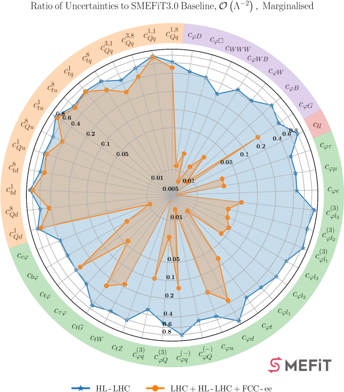
Figure 4.1: Same as Fig. 3.8 for the marginalised bounds on the SMEFT operators from a global $\mathcal{O}\left(\Lambda^{-2}\right)$ analysis, displaying the ratio of uncertainties to the SMEFiT3.0 baseline of fits which include first the HL-LHC projections and subsequently both the HL-LHC and the FCC-ee observables. All fits shown here are carried out based on Level-1 pseudo-data.

Next we quantify the impact on the EFT coefficients of measurements from the FCC-ee and CEPC when added on top of the baseline fit extended with the HL-LHC projections discussed in Sect. 3.3. Since our projections reproduce the assumed SM theory for the fitted observables by construction, one is interested only in the reduction of the length of the 95% CL interval for the relevant operators, as quantified by the ratio $R_{\delta c_{i}}$ in Eq. (3.2), and hence we do not display the fit central values. We focus first on the FCC-ee, and then compare with the CEPC results.

Fig. 4.1 (4.3) displays, in the same format as that of Fig. 3.8, the marginalised bounds on the SMEFT operators from a global linear (quadratic) analysis, displaying the ratio of uncertainties to the SMEFiT3.0 baseline of fits which include, first, the HL-LHC projections, and subsequently, both the HL-LHC and the FCC-ee observables, see Table A.1. Inspection of Fig. 4.1 demonstrates the substantial impact that FCC-ee measurements would provide on the SMEFT parameter space in comparison with a post-HL-LHC baseline. Indeed, the FCC-ee would constrain a wide range of directions in the EFT coefficients, except for the four-quark operators. For the latter only moderate indirect improvements are expected, which go away in the quadratic fits shown in Fig. 4.3. This is due to the fact that no FCC-ee observables included in the fit are sensitive to four-quark operators, and thus any impact of FCC-ee on their constraints arises through marginalisation.

From Fig. 4.1 one also observes how the bounds on some of the purely bosonic, four-lepton, and two-fermion operators achieved at the FCC-ee could improve on the HL-LHC ones by almost two orders of magnitude. For instance, the 95% CL interval for the coefficient $c_{WWW}$, which modifies the triple gauge boson interactions, is reduced by a factor $R_{\delta c_{i}}\simeq 0.3$ at the end of HL-LHC and then down to $R_{\delta c_{i}}=0.008$ at the FCC-ee, corresponding to a relative improvement on the bound by a factor around $40$. Likewise, our analysis finds values of $R_{\delta c_{i}}\simeq 0.4,\,0.4$ and $0.6$ at the end of the HL-LHC for the coefficients $c_{\varphi e}$, $c_{c\varphi}$, and $c_{\varphi B}$ respectively, which subsequently go down to $R_{\delta c_{i}}\simeq 0.005,\,0.01$ and $0.008$ upon the inclusion of the FCC-ee pseudo-data. This translates into relative improvements by factors of around $80$, $40$, and $70$ for each EFT coefficient, respectively. While these are only representative examples, they highlight how precision measurements at FCC-ee will provide stringent constraints on the SMEFT parameter space, markedly improving on the limits achievable at the HL-LHC.

In Figs. 4.1 and 4.3, the impact of the FCC-ee measurements on the EFT coefficients is presented in terms of the relative improvement with respect to either the SMEFiT3.0 baseline or its variant accounting also for the HL-LHC projections. In order to compare with previous related studies, it is useful to also provide the absolute magnitude of the resulting bounds, in addition to their relative improvement as compared to the baseline. With this motivation, Table 4.2 indicates the 95% CL upper bounds on the EFT coefficients obtained from the fits including both the HL-LHC and the FCC-ee projections, assuming $\Lambda=1$ TeV. In analogy with Table 3.4, we provide these bounds for linear and quadratic EFT fits and both at the individual and marginalised level. The impact of the FCC-ee is clearly visible specially for the purely bosonic and two-fermion operators, with most of them constrained to be $|c|\mathrel{\hbox to0.0pt{\lower 4.0pt\hbox{\hskip 1.0pt$\sim$}\hss}\raise 1.0pt\hbox{$<$}}0.1$ (for $\Lambda=1$ TeV) in the global marginalised fit, and several of them at the $|c|\mathrel{\hbox to0.0pt{\lower 4.0pt\hbox{\hskip 1.0pt$\sim$}\hss}\raise 1.0pt\hbox{$<$}}10^{-2}$ level or better. We demonstrate in Sect. 5 how these constraints on the Wilson coefficients translate into the mass reach for UV-complete models.

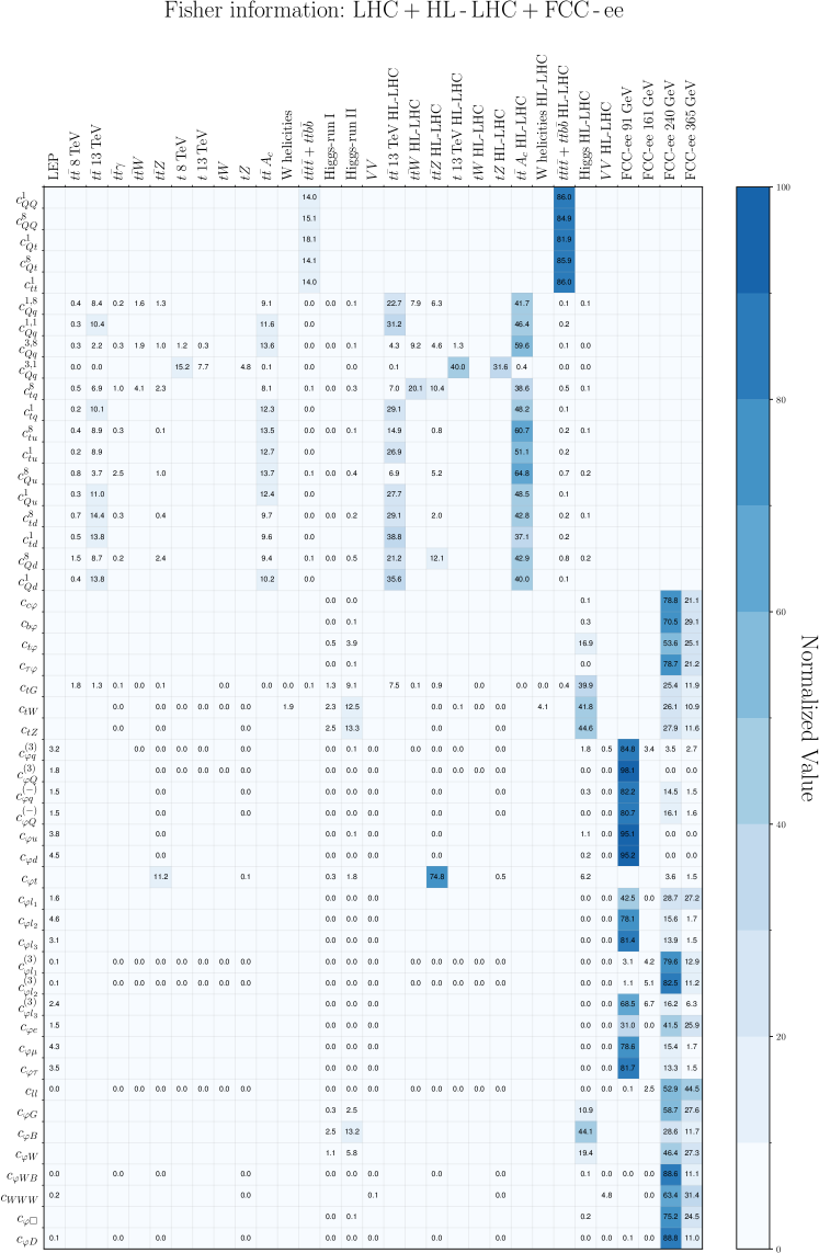
Figure 4.2: Diagonal entries of the Fisher information matrix evaluated at $\mathcal{O}\left(\Lambda^{-2}\right)$ in the EFT expansion, Eq. (4.4), for the complete dataset (LEP EWPOs + LHC_Run1 + LHC_Run2 + HL-LHC + FCC-ee) considered in this work. Each row is normalised to 100. The LHC_Run2 and HL-LHC datasets are displayed separately. For the FCC-ee observables, we evaluate the Fisher matrix individually for each of the relevant $\sqrt{s}$ values. Empty entries indicate lack of direct sensitivity, while “0.0” entries indicate a non-zero sensitivity which is less than 0.05% in magnitude.

Class	DoF	95% CL bounds, $\mathcal{O}\left(\Lambda^{-2}\right)$		95% CL bounds, $\mathcal{O}\left(\Lambda^{-4}\right)$,
		Individual	Marginalised	Individual	Marginalised
2FB	$c_{c\varphi}$	2.82$\cdot 10^{-3}$	3.69$\cdot 10^{-3}$	2.79$\cdot 10^{-3}$	3.68$\cdot 10^{-3}$
	$c_{b\varphi}$	1.9$\cdot 10^{-3}$	3.61$\cdot 10^{-3}$	1.87$\cdot 10^{-3}$	3.4$\cdot 10^{-3}$
	$c_{t\varphi}$	2.96$\cdot 10^{-1}$	2.18	2.88$\cdot 10^{-1}$	2.19
	$c_{\tau\varphi}$	1.92$\cdot 10^{-3}$	2.85$\cdot 10^{-3}$	1.93$\cdot 10^{-3}$	2.79$\cdot 10^{-3}$
	$c_{tG}$	2.38$\cdot 10^{-2}$	6.89$\cdot 10^{-2}$	2.45$\cdot 10^{-2}$	6.52$\cdot 10^{-2}$
	$c_{tW}$	3.83$\cdot 10^{-3}$	5.82$\cdot 10^{-2}$	3.74$\cdot 10^{-3}$	6.02$\cdot 10^{-2}$
	$c_{tZ}$	4.79$\cdot 10^{-3}$	6.92$\cdot 10^{-2}$	4.7$\cdot 10^{-3}$	7.19$\cdot 10^{-2}$
	$c_{\varphi q}^{(3)}$	4.9$\cdot 10^{-3}$	1.39$\cdot 10^{-2}$	4.84$\cdot 10^{-3}$	1.29$\cdot 10^{-2}$
	$c_{\varphi Q}^{(3)}$	5.28$\cdot 10^{-3}$	3.5$\cdot 10^{-2}$	5.32$\cdot 10^{-3}$	1.92$\cdot 10^{-2}$
	$c_{\varphi q}^{(-)}$	2.89$\cdot 10^{-2}$	6.03$\cdot 10^{-2}$	2.88$\cdot 10^{-2}$	4.06$\cdot 10^{-2}$
	$c_{\varphi Q}^{(-)}$	9.37$\cdot 10^{-3}$	2.46$\cdot 10^{-2}$	9.69$\cdot 10^{-3}$	2.44$\cdot 10^{-2}$
	$c_{\varphi u}$	2.99$\cdot 10^{-2}$	1.54$\cdot 10^{-1}$	2.99$\cdot 10^{-2}$	8.18$\cdot 10^{-2}$
	$c_{\varphi d}$	4.62$\cdot 10^{-2}$	3.74$\cdot 10^{-1}$	4.47$\cdot 10^{-2}$	1.65$\cdot 10^{-1}$
	$c_{\varphi t}$	3.72$\cdot 10^{-1}$	6.65$\cdot 10^{-1}$	3.76$\cdot 10^{-1}$	6.55$\cdot 10^{-1}$
	$c_{\varphi l_{1}}$	2.38$\cdot 10^{-3}$	4.59$\cdot 10^{-3}$	2.39$\cdot 10^{-3}$	4.38$\cdot 10^{-3}$
	$c_{\varphi l_{2}}$	1.03$\cdot 10^{-2}$	2.55$\cdot 10^{-2}$	1.01$\cdot 10^{-2}$	2.56$\cdot 10^{-2}$
	$c_{\varphi l_{3}}$	1.05$\cdot 10^{-2}$	2.79$\cdot 10^{-2}$	1.06$\cdot 10^{-2}$	2.8$\cdot 10^{-2}$
	$c_{\varphi l_{1}}^{(3)}$	8.97$\cdot 10^{-4}$	7.45$\cdot 10^{-3}$	8.93$\cdot 10^{-4}$	7.06$\cdot 10^{-3}$
	$c_{\varphi l_{2}}^{(3)}$	9.79$\cdot 10^{-4}$	8.1$\cdot 10^{-3}$	9.73$\cdot 10^{-4}$	7.8$\cdot 10^{-3}$
	$c_{\varphi l_{3}}^{(3)}$	8.59$\cdot 10^{-3}$	1.97$\cdot 10^{-2}$	8.72$\cdot 10^{-3}$	1.86$\cdot 10^{-2}$
	$c_{\varphi e}$	2.52$\cdot 10^{-3}$	4.62$\cdot 10^{-3}$	2.54$\cdot 10^{-3}$	4.62$\cdot 10^{-3}$
	$c_{\varphi\mu}$	1.18$\cdot 10^{-2}$	3.0$\cdot 10^{-2}$	1.24$\cdot 10^{-2}$	3.02$\cdot 10^{-2}$
	$c_{\varphi\tau}$	1.28$\cdot 10^{-2}$	3.01$\cdot 10^{-2}$	1.29$\cdot 10^{-2}$	2.95$\cdot 10^{-2}$
2L2H	$c_{Qq}^{1,8}$	2.59$\cdot 10^{-1}$	2.34	3.06$\cdot 10^{-1}$	4.69$\cdot 10^{-1}$
	$c_{Qq}^{1,1}$	5.81$\cdot 10^{-1}$	1.16$\cdot 10^{1}$	3.64$\cdot 10^{-1}$	2.82$\cdot 10^{-1}$
	$c_{Qq}^{3,8}$	7.95$\cdot 10^{-1}$	3.96	6.56$\cdot 10^{-1}$	5.34$\cdot 10^{-1}$
	$c_{Qq}^{3,1}$	1.27$\cdot 10^{-1}$	1.27$\cdot 10^{-1}$	1.3$\cdot 10^{-1}$	1.14$\cdot 10^{-1}$
	$c_{tq}^{8}$	4.12$\cdot 10^{-1}$	2.65	4.55$\cdot 10^{-1}$	5.14$\cdot 10^{-1}$
	$c_{tq}^{1}$	4.83$\cdot 10^{-1}$	6.87	2.83$\cdot 10^{-1}$	2.19$\cdot 10^{-1}$
	$c_{tu}^{8}$	4.38$\cdot 10^{-1}$	6.97	5.83$\cdot 10^{-1}$	7.19$\cdot 10^{-1}$
	$c_{tu}^{1}$	8.81$\cdot 10^{-1}$	1.89$\cdot 10^{1}$	4.57$\cdot 10^{-1}$	3.57$\cdot 10^{-1}$
	$c_{Qu}^{8}$	7.51$\cdot 10^{-1}$	6.81	7.44$\cdot 10^{-1}$	8.21$\cdot 10^{-1}$
	$c_{Qu}^{1}$	6.8$\cdot 10^{-1}$	8.65	3.5$\cdot 10^{-1}$	2.68$\cdot 10^{-1}$
	$c_{td}^{8}$	9.38$\cdot 10^{-1}$	1.32$\cdot 10^{1}$	1.35	1.03
	$c_{td}^{1}$	1.79	2.94$\cdot 10^{1}$	6.2$\cdot 10^{-1}$	4.61$\cdot 10^{-1}$
	$c_{Qd}^{8}$	1.43	9.3	1.32	1.27
	$c_{Qd}^{1}$	1.49	2.32$\cdot 10^{1}$	5.0$\cdot 10^{-1}$	3.96$\cdot 10^{-1}$
4H	$c_{QQ}^{1}$	7.71	—	1.94	6.75
	$c_{QQ}^{8}$	2.15$\cdot 10^{1}$	—	5.82	2.02$\cdot 10^{1}$
	$c_{Qt}^{1}$	2.95$\cdot 10^{2}$	—	1.65	1.36
	$c_{Qt}^{8}$	6.74	—	3.44	2.75
	$c_{tt}^{1}$	3.77	—	9.62$\cdot 10^{-1}$	8.01$\cdot 10^{-1}$
4L	$c_{ll}$	6.98$\cdot 10^{-4}$	8.05$\cdot 10^{-4}$	6.99$\cdot 10^{-4}$	8.06$\cdot 10^{-4}$
B	$c_{\varphi G}$	9.83$\cdot 10^{-4}$	6.22$\cdot 10^{-3}$	9.63$\cdot 10^{-4}$	6.34$\cdot 10^{-3}$
	$c_{\varphi B}$	1.97$\cdot 10^{-3}$	6.65$\cdot 10^{-3}$	1.97$\cdot 10^{-3}$	6.67$\cdot 10^{-3}$
	$c_{\varphi W}$	5.13$\cdot 10^{-3}$	2.27$\cdot 10^{-2}$	5.1$\cdot 10^{-3}$	1.98$\cdot 10^{-2}$
	$c_{\varphi WB}$	2.77$\cdot 10^{-4}$	1.33$\cdot 10^{-2}$	2.73$\cdot 10^{-4}$	1.32$\cdot 10^{-2}$
	$c_{WWW}$	7.17$\cdot 10^{-3}$	7.83$\cdot 10^{-3}$	7.03$\cdot 10^{-3}$	7.88$\cdot 10^{-3}$
	$c_{\varphi\Box}$	3.91$\cdot 10^{-2}$	7.0$\cdot 10^{-2}$	4.0$\cdot 10^{-2}$	6.72$\cdot 10^{-2}$
	$c_{\varphi D}$	6.1$\cdot 10^{-4}$	2.45$\cdot 10^{-2}$	6.05$\cdot 10^{-4}$	2.46$\cdot 10^{-2}$

Table 4.2: The 95% CL upper bounds on the EFT coefficients obtained from the fits including both the HL-LHC and the FCC-ee (Level-1) pseudo-data, see also Figs. 4.1 and 4.3 for the corresponding graphical representation (relative to the baseline bounds), for $\Lambda=1$ TeV. We present results both for linear and quadratic EFT fits and at the individual and marginalised level, in analogy with Table 3.4 for the baseline SMEFiT3.0 analysis.

Fisher information analysis.

In order to better scrutinise the interplay between the constraints provided by the (HL-)LHC measurements, on the one hand, and by the FCC-ee ones, on the other hand, it is illustrative to evaluate the Fisher information matrix Ethier:2021bye ; Ellis:2020unq . The entries of the Fisher information matrix at $\mathcal{O}\left(\Lambda^{-2}\right)$ in the EFT expansion are given by

$$I_{ij}=\sum_{m=1}^{n_{\rm dat}}\frac{\sigma^{\rm(eft)}_{m,i}\sigma^{\rm(eft)}_{m,j}}{\delta_{{\rm exp},m}^{2}}\,,\qquad i,j=1,\ldots,n_{\rm eft},$$ (4.4)

with $\sigma^{\rm(eft)}_{m,i}$ being the linear EFT correction to the SM cross-section for the $m$-th data point associated to the $i$-th Wilson coefficient, and $\delta_{{\rm exp},m}$ indicates the total experimental uncertainty. Eq. (4.4) should be evaluated separately for each dataset or group of processes entering the analysis; the larger the value of the diagonal entry $I_{ii}$, the more impactful this dataset will be for the $i$-th EFT coefficient.

Fig. 4.2 displays the diagonal entries of the linear Fisher information matrix, Eq. (4.4), computed over the complete dataset considered in this work: LEP EWPOs, LHC_Run1, LHC_Run2, HL-LHC, and the FCC-ee. In this plot each row is normalised to 100. Note that the LHC Run II datasets and the HL-LHC projections are displayed separately. For the FCC-ee projections, we evaluate the Fisher matrix individually for each of the relevant $\sqrt{s}$ values.

From the entries of the Fisher information matrix it can be observed how for all LHC processes being considered, the HL-LHC projections display the largest Fisher information, reflecting the expected reduction of statistical and systematic uncertainties. The table also confirms that the LEP EWPOs carry a small amount of information once the FCC-ee projections are included in the fit. Within the global EFT fit, the FCC-ee observables would provide the dominant constraints for all the two-fermion and purely bosonic operators, except for $c_{tG}$, $c_{tW}$, $c_{tZ}$, $c_{\varphi B}$, and $c_{\varphi t}$, where the constraints from HL-LHC processes are still expected to dominate. The two-light-two-heavy operators are entirely dominated by HL-LHC, mostly from inclusive $t\bar{t}$ production and by the charge asymmetry measurements $A_{C}$.

Concerning the impact of the FCC-ee datasets for different center-of-mass energies, Fig. 4.2 reveals that the bulk of the constraints on the SMEFT parameter space should be provided by the runs at $\sqrt{s}=91$ GeV and at $\sqrt{s}=240$ GeV, with relevant information arising also from the $\sqrt{s}=365$ GeV run. Fig. 4.2 highlights the interplay between runs at different values of $\sqrt{s}$ to constrain new physics through the SMEFT interpretation: when their information is combined, the resulting picture is sharper than that of any individual run. On the other hand, only moderate information would be provided by the run at the $WW$ threshold ($\sqrt{s}=161$ GeV), and even for the triple gauge operator coefficient $c_{WWW}$ it would be the $Zh$ run that dominates the sensitivity. Hence, from the viewpoint of EFT analyses, the $\sqrt{s}=161$ GeV run appears to be the less impactful.

The Fisher information matrix shown in Fig. 4.2 quantifies the relative sensitivity of various processes to specific operators based on their linear EFT contributions, and corresponds to what one would expect to find in linear individual fits. However, it cannot capture the complete picture encompassed by the global fit at the marginalised level, and in particular it does not account for the information on the correlations between operators. Indeed, in the marginalised fits, these correlations will often modify the picture as compared with expectations based on the Fisher information matrix. We also note that Eq. (4.4) receives additional contributions when evaluated for quadratic EFT fits, which are not necessarily subdominant in comparison with the linear contributions.

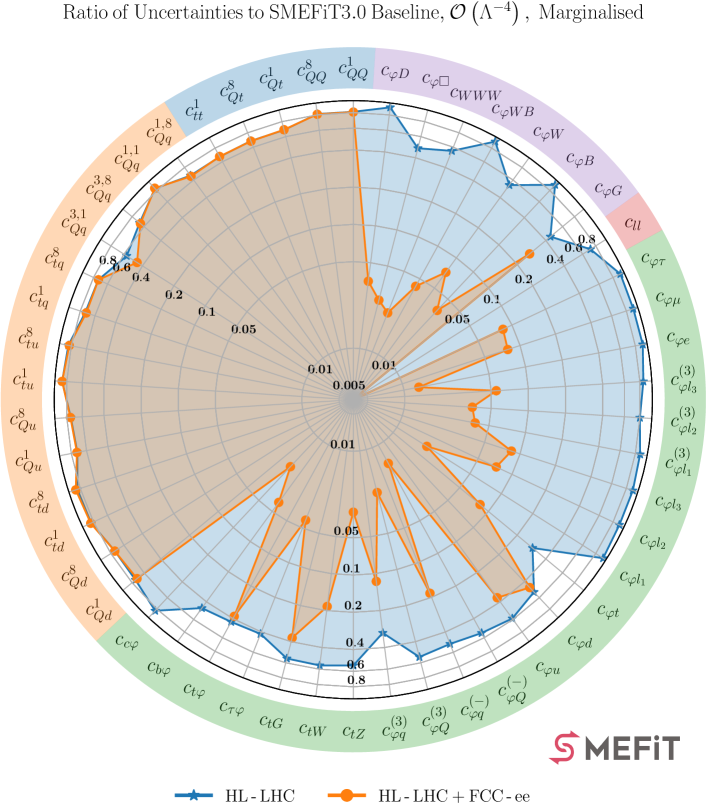
Figure 4.3: Same as Fig. 4.1 in the case of the fits with EFT cross-sections including both the linear, $\mathcal{O}\left(\Lambda^{-2}\right)$, and the quadratic, $\mathcal{O}\left(\Lambda^{-4}\right)$, corrections associated to the dimension-six operators considered in the analysis.

Impact of quadratic EFT corrections.

The analog of Fig. 4.1 in the case of EFT fits with quadratic corrections is displayed in Fig. 4.3. Also here one observes a significant reduction of the bounds on the EFT coefficients upon inclusion of the FCC-ee observables. The improvements observed for some four-quark operators in the linear fit of Fig. 4.1 mostly disappear when including quadratic corrections demonstrating that the improvement of the linear fit constraints arise from indirect correlations with other degrees of freedom. Indeed, the quadratic fit result illustrates how the FCC-ee observables do not have any direct sensitivity on the four-quark operators, both for the two-light-two-heavy and for the four-heavy ones.

From Table 4.2 one notices that the differences between linear and quadratic bounds are in general reduced as compared to the case of the SMEFiT3.0 results collected in Table 3.4. This feature is explained by the improved precision of the FCC-ee measurements: since we assume the SM in the pseudo-data, the best-fit values of the Wilson coefficients move closer to zero with smaller uncertainties, and hence the quadratic terms become less significant. We note however that for a subset of operators, such as the two-light-two-heavy ones, which are not constrained by the FCC-ee measurements the discrepancy between linear and quadratic remains large.

Disentangling the impact of datasets with fixed $\sqrt{s}$.

As indicated in Table 4.1, the FCC-ee plans to operate sequentially, collecting data at different center-of-mass energies, $\sqrt{s}$, starting at the $Z$-pole and then increasing the energy up to the $t\bar{t}$ threshold. Plans to define different running scenarios are also being considered, for example directly starting as a Higgs factory with the $\sqrt{s}=240$ GeV run and only later running at the $Z$-pole energy. It is therefore relevant to disentangle, at the level of the global SMEFT fit, the separate impact of datasets with a given $\sqrt{s}$ value to evaluate the advantages and disadvantages of the proposed running scenarios, see also the Fisher information matrix in Fig. 4.2.

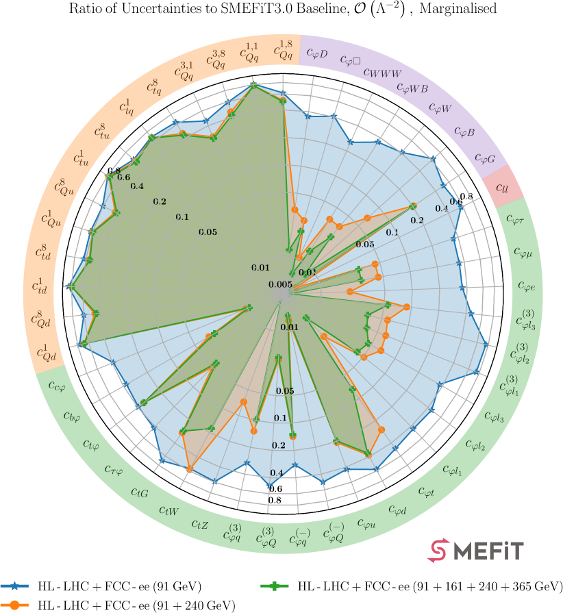
Figure 4.4: Same as Fig. 4.1, now comparing the sequential impact of the separate $\sqrt{s}$ runs at the FCC-ee with respect to the baseline fit. We display the effects of adding the projected FCC-ee dataset at, first, $\sqrt{s}=91$ GeV (blue), followed by adding $\sqrt{s}=240$ GeV (orange) and finally adding both $\sqrt{s}=161$ and 365 GeV (green), which completes the FCC-ee dataset listed in Table 4.1.

Fig. 4.4 illustrates the sequential impact of the datasets collected at different values of $\sqrt{s}$ at the FCC-ee. First we show the values of the ratio $R_{\delta c_{i}}$ when only the $Z$-pole EWPOs at $\sqrt{s}=91$ GeV are included in the fit, then when also the Higgs factory dataset from the $\sqrt{s}=240$ GeV is accounted for, and finally for the full FCC-ee dataset, which includes also the $WW$ run at 161 GeV and the $t\bar{t}$ run at 365 GeV. Fig. 4.4 indicates that the largest impact is obtained when the Higgs, diboson, and fermion-pair production data collected at 240 GeV are included in the fit together with the $Z$-pole run. We also observe how the measurements from the $\sqrt{s}=161$ GeV and 365 GeV runs are necessary to achieve the ultimate constraining potential of the FCC-ee in the EFT parameter space, with several operators experiencing a marked improvement of the associated bounds. This breakdown demonstrates the interplay between the information provided by the FCC-ee runs at the various proposed center-of-mass energies.

FCC-ee impact compared to the CEPC.

We next study the impact of the CEPC measurements on the SMEFT coefficients, relative to that obtained in the FCC-ee case and shown in Fig. 4.1. Fig. 4.5 displays the constraints provided by both colliders when added on top of the same HL-LHC baseline dataset, always relative to the SMEFiT3.0 baseline fit. In general, a similar constraining power is obtained, consistent with the lack of major differences between their running plans (see Table 4.1), though the FCC-ee bounds tend to be better than those from CEPC. The same qualitative conclusions are obtained in the case in which the analysis of Fig. 4.5 is carried with quadratic EFT corrections.

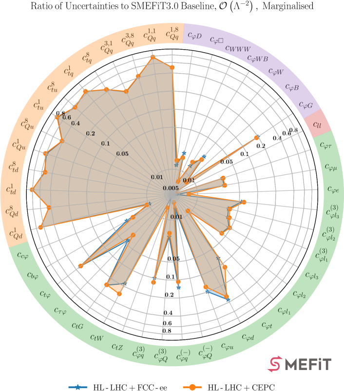
Figure 4.5: Same as Fig. 4.1 now comparing the impact of the FCC-ee and CEPC datasets.

When performing this comparison, we noticed that the total experimental uncertainties provided by the FCC-ee and CEPC collaborations for the Snowmass study, which we adopt in our analysis, differ by more than the scaling of integrated luminosities, as would be expected in the case of purely statistical uncertainties without further correction factors. This is illustrated by the Fisher information matrix, defined in Eq. (4.4) at the linear EFT level, when evaluated in terms of ratios between the two experiments. If one takes the ratio of the diagonal entries of the Fisher information matrix between the FCC-ee and the CEPC, given that both colliders share the same theory predictions, one obtains

$$I_{ii}^{\rm(FCC-ee)}/I_{ii}^{\rm(CEPC)}=\sum_{m=1}^{n_{\rm dat}}\left(\delta_{{\rm exp},m}^{2}\right)_{\rm CEPC}\Bigg{/}\sum_{m^{\prime}=1}^{n_{\rm dat}}\left(\delta_{{\rm exp},m^{\prime}}^{2}\right)_{\rm FCC-ee}\,,\qquad i=1,\ldots,n_{\rm eft},$$ (4.5)

namely the ratio of total experimental uncertainties squared. For observables with only statistical uncertainties, and assuming that eventual acceptance corrections cancel out, this ratio should reproduce the corresponding ratios of integrated luminosities reported in Table 4.1, that is,

$$I_{ii}^{\rm(FCC-ee)}/I_{ii}^{\rm(CEPC)}\simeq\left(\mathcal{L}_{\rm FCC-ee}/\mathcal{L}_{\rm CEPC}\right)\,.$$ (4.6)

Fig. 4.6 displays the ratio defined in Eq. (4.5), evaluated separately for the observables entering the four data-taking periods considered. Values of Eq. (4.5) below unity indicate EFT coefficients for which the CEPC observables should be more constraining than the FCC-ee ones. A deviation from the luminosity scaling for the $\sqrt{s}=91$ GeV run is expected, and indeed observed, since each collaboration makes different assumptions for their systematic uncertainties. On the other hand, since at $\sqrt{s}=161,240$ and 365 GeV the uncertainties considered are purely statistical, for these observables the ratios in Fig. 4.6 are expected to follow Eq. (4.6). While in some cases this in indeed true, in particular for the runs at $\sqrt{s}=161$ GeV and $240$ GeV, in other cases there are larger differences. Particularly noticeable are those arising in the data-taking period at $\sqrt{s}=365$ GeV. There one expects a ratio of around $3$ purely on the luminosity scaling, but actually one obtains a range of values between 0.9 and 6.6.

It is beyond the scope of this work to scrutinise the origin of these differences: they could be explained by different assumptions on the experimental selection procedure and acceptance cuts, for example. Nevertheless, the analysis of Fig. 4.6 highlights that in general the relative impact in the SMEFT parameter space of the projected FCC-ee and CEPC pseudo-data differs from the expectations based on a pure luminosity scaling.

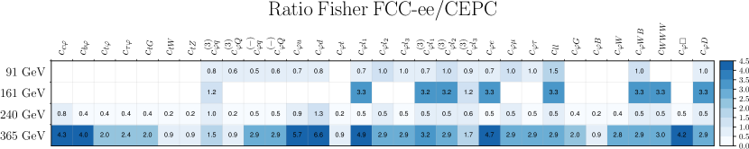
Figure 4.6: The ratio of the entries of the Fisher information matrix between the FCC-ee and the CEPC, Eq. (4.5), evaluated separately for the observables entering the four center of mass energies $\sqrt{s}$ considered. Since projections for both colliders share theory predictions, this ratio is equivalent to the ratio of total experimental uncertainties squared. In turn, if the latter contains only the statistical uncertainties, the entries of the table should match the corresponding ratios of integrated luminosities from Table 4.1.

5 Constraints on UV-complete models through the SMEFT

We now quantify the constraints that LHC Run II measurements and future collider projections impose on the parameter space of representative UV-complete scenarios. To this aim, we benefit from the integration of SMEFiT with matchmakereft Carmona:2021xtq via the Match2Fit interface presented in terHoeve:2023pvs . We consider results for the (indirect) mass reach for new heavy particles at the HL-LHC and FCC-ee obtained from the tree-level matching of a wide range of one-particle extensions of the SM. We also present results for the reach in the UV couplings for the one-loop matching of a subset of the same one-particle extensions and for the tree-level matching of a multi-particle extension of the SM. The corresponding results for the CEPC are qualitatively similar to the FCC-ee ones, consistently with Fig. 4.5, and hence are not shown here.

Model Label	SM irreps	UV couplings
Heavy Scalar Models
$\mathcal{S}$	$(1,1)_{0\phantom{/-3}}$	$\kappa_{\mathcal{S}}$
$\phi$	$(1,2)_{1/2\phantom{-}}$	$\lambda_{\phi},\,\,(y_{\phi}^{u})_{33}$
$\Xi$	$(1,3)_{0\phantom{/-3}}$	$\kappa_{\Xi}$
$\Xi$	$(1,3)_{1\phantom{/-3}}$	$\kappa_{\Xi_{1}}$
$\omega_{1}$	$(3,1)_{-1/3}$	$\left(y_{\omega_{1}}^{qq}\right)_{33}$
$\omega_{4}$	$(3,1)_{-4/3}$	$\left(y_{\omega_{4}}^{uu}\right)_{33}$
$\zeta$	$(3,3)_{-1/3}$	$\left(y_{\zeta}^{qq}\right)_{33}$
$\Omega_{1}$	$(6,1)_{1/3\phantom{-}}$	$\left(y_{\Omega_{1}}^{qq}\right)_{33}$
$\Omega_{4}$	$(6,1)_{4/3\phantom{-}}$	$\left(y_{\omega_{4}}\right)_{33}$
$\Upsilon$	$(6,3)_{1/3\phantom{-}}$	$\left(y_{\Upsilon}\right)_{33}$
$\Phi$	$(8,2)_{1/2\phantom{-}}$	$\left(y_{\Phi}^{qu}\right)_{33}$
Heavy Vector Models
$\mathcal{B}_{1}$	$(1,1)_{1\phantom{/-3}}$	$g_{B_{1}}^{\varphi}$
$\mathcal{W}$	$(1,3)_{0\phantom{/-3}}$	$\left(g_{\mathcal{W}}^{\ell}\right)_{11},\,\left(g_{\mathcal{W}}^{\ell}\right)_{22}$, $g_{\mathcal{W}}^{\varphi}$, $\left(g_{\mathcal{W}}^{q}\right)_{33}$
$\mathcal{W}_{1}$	$(1,3)_{1\phantom{/-3}}$	$g_{\mathcal{W}_{1}}^{\varphi}$
$\mathcal{H}$	$(8,3)_{0\phantom{/-3}}$	$\left(g_{\mathcal{H}}\right)_{33}$
$\mathcal{Q}_{5}$	$(3,2)_{-5/6}$	$\left(g_{\mathcal{Q}_{5}}^{uq}\right)_{33}$
$\mathcal{Y}_{5}$	$(\bar{6},2)_{-5/6}$	$\left(g_{\mathcal{Y}_{5}}\right)_{33}$
Heavy Fermion Models
$N$	$(1,1)_{0\phantom{/-3}}$	$\left(\lambda_{N}^{e}\right)_{3}$
$E$	$(1,1)_{-1\phantom{/3}}$	$\left(\lambda_{E}\right)_{3}$
$\Delta_{1}$	$(1,2)_{-1/2}$	$\left(\lambda_{\Delta_{1}}\right)_{3}$
$\Delta_{3}$	$(1,2)_{-3/2}$	$\left(\lambda_{\Delta_{3}}\right)_{3}$
$\Sigma$	$(1,3)_{0\phantom{/-3}}$	$\left(\lambda_{\Sigma}\right)_{3}$
$\Sigma_{1}$	$(1,3)_{-1\phantom{/3}}$	$\left(\lambda_{\Sigma_{1}}\right)_{3}$
$U$	$(3,1)_{2/3\phantom{-}}$	$\left(\lambda_{U}\right)_{3}$
$D$	$(3,1)_{-1/3}$	$\left(\lambda_{D}\right)_{3}$
$Q_{1}$	$(3,2)_{1/6\phantom{-}}$	$\left(\lambda_{Q_{1}}^{u}\right)_{3}$
$Q_{7}$	$(3,2)_{7/6\phantom{-}}$	$\left(\lambda_{Q_{7}}\right)_{3}$
$T_{1}$	$(3,3)_{-1/3}$	$\left(\lambda_{T_{1}}\right)_{3}$
$T_{2}$	$(3,3)_{2/3\phantom{-}}$	$\left(\lambda_{T_{2}}\right)_{3}$

Table 5.1: The one-particle UV-complete models that are considered in this work and matched to the SMEFT at tree level. For the $\phi$ (heavy scalar) and $T_{1}$ and $T_{2}$ (heavy fermion) models, we also provide results based on one-loop matching. For each model, following terHoeve:2023pvs ; deBlas:2017xtg we indicate its label, the gauge group representation of the new heavy particle in the notation $(\textrm{SU}(3),\textrm{SU}(2))_{\textrm{U}(1)}$, and the relevant UV couplings entering the associated Lagrangian. The model couplings are restricted to respect the SMEFiT flavour assumption after tree-level matching. Multi-particle models can be constructed from combining subsets of the one-particle models.

Tree-level matching of one-particle extensions.

First, we provide results for the UV-complete one-particle models considered in terHoeve:2023pvs , each of them associated to a different gauge group representation of the new heavy particle, matched at tree-level to the SMEFT. Table 5.1 displays the one-particle models considered in this work, indicating their label, the SM gauge group representation of the new heavy particle, and the UV couplings entering the associated Lagrangian (following the convention in deBlas:2017xtg ). We restrict the possible UV couplings to ensure consistency with the SMEFiT flavour assumption after tree-level matching.

To illustrate the reach of the FCC-ee measurements on the parameter space of these UV models, we derive lower bounds on the mass of the heavy particle $M_{\rm UV}$ for each of the one-particle extensions listed in Table 5.1 by assuming a given value for the corresponding UV couplings $g_{\rm UV}$. For simplicity, we consider only models with a single UV coupling. The projected $95\%$ CL lower bounds on $M_{\rm UV}$ at FCC-ee are shown in Fig 5.1 for two limiting assumptions on the value of UV couplings: $g_{\rm UV}=1$ and $g_{\rm UV}=4\pi$. The chosen values are on the upper edge of what can be considered as weakly and strongly coupled, and in fact, $g_{\rm UV}>4\pi$ would violate the perturbative limit. For each model, we present results for a SMEFT analysis based on Level-1 pseudo-data of the current dataset, LEP+LHC${}_{\rm Run\,II}$, and then for its extension first with HL-LHC projections, and subsequently with the complete set of FCC-ee observables.

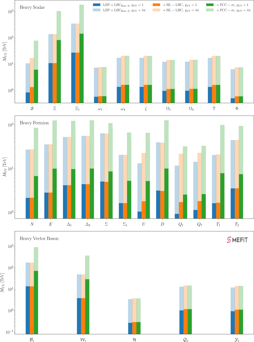
Figure 5.1: The 95% CL lower bounds on the heavy particle mass $M_{\rm UV}$ for the one-particle UV-completions of the SM considered in this work, matched to the SMEFT using tree-level relations. In all cases we include corrections up to quadratic order in the EFT expansion. From top to bottom, we display results for models with heavy scalars, heavy fermions, and heavy vector bosons, see Table 5.1 for the definition of each model. We present results for SMEFT analyses based on the current dataset (LEP+LHC_RunII), then for its extension first with HL-LHC projections, and subsequently with the full set of FCC-ee observables. We consider two scenarios for the UV coupling constants, $g_{\rm UV}=1$ (darker) and $g_{\rm UV}=4\pi$ (lighter). Note the logarithmic scale of the $y$-axis.

Several observations can be drawn from perusing the results of Fig. 5.1. On the one hand, we find that the HL-LHC projections improve the mass reach for several models, in particular those that include heavy quark partners such as $U$, $Q_{1}$, and $Q_{7}$. On the other hand, the models that are not affected by HL-LHC fall into two distinct categories. One is composed of models such as $N$, $E$, $\Delta_{1,3}$, $\Sigma$, $\Sigma_{1}$, and $D$, that generate a subset of operators which display no improved sensitivity in individual fits to HL-LHC pseudo-data, namely purely leptonic and bosonic operators probed by EWPOs as well as $c_{\varphi Q}^{(-)}$ and $c_{\varphi Q}^{(3)}$. The other class contains the models $\Xi$, $\Xi_{1}$, $T_{2}$, $\mathcal{B}_{1}$, and $\mathcal{W}_{1}$ that do generate operators that have associated improved bounds at the HL-LHC, but where the sensitivity to the UV parameters is driven by operators that are instead insensitive to HL-LHC data, such as $c_{\varphi D}$, $c_{\varphi Q}^{(-)}$ or $c_{\varphi Q}^{(3)}$.

The mass reach enabled by FCC-ee measurements increases markedly for several models as compared to the post-HL-LHC limits, in some cases by up to an order of magnitude. The largest effects are observed for the UV scenarios that modify the interactions of Higgs and electroweak bosons, which are tightly constrained by the FCC-ee data. These include the $\mathcal{S}$, $\Xi$, and $\Xi_{1}$ heavy scalar models; the $N$, $E$, $\Delta_{1}$, $U$, $D$, $T_{1}$, and $T_{2}$ vector-like heavy fermion models; and the $\mathcal{B}_{1}$ and $\mathcal{W}_{1}$ heavy vector boson models. For other scenarios, such as those primarily modifying the four-quark interaction vertices, there is only a marginal information gain provided by FCC-ee measurements, consistently with the findings at the Wilson coefficient level in Fig. 4.1.

In terms of the heavy particle mass reach, we observe that FCC-ee measurements will be sensitive to BSM scales of up to around 100 TeV, 10 TeV, and 70 TeV for some of the studied heavy scalar, fermion, and vector boson UV-completions respectively, in the case of $g_{\rm UV}=1$. This sensitivity increases to around $10^{3}$ TeV, 200 TeV, and 800 TeV in the case of strongly coupled one-particle extensions of the SM in the upper limit of the perturbative regime, $g_{\rm UV}=4\pi$. One also observes how, at least for the one-particle extensions considered here, at the HL-LHC there is not a large difference between the mass reach associated to direct production (with $m_{X}\sim 7$ TeV at most) and that associated to the indirect bounds obtained in the EFT framework. On the other hand, at the FCC-ee the production of new heavy (TeV-scale) particles consistent with the LHC exclusion bounds is kinematically impossible due to the limited $\sqrt{s}$ values available, while the EFT bounds instead reach much higher energies, as illustrated by the examples of Fig. 5.1. This result further confirms the powerful sensitivity to heavy new physics enabled by the high-precision electroweak, Higgs, and top quark measurements to be performed at the FCC-ee highlighted by previous studies.

One-loop matched and multi-particle models.

Following the discussion on single-particle extensions of the SM matched at tree level, we now evaluate the impact of the FCC-ee data on more general UV completions. We consider in particular the heavy scalar $\phi$ and the heavy fermion $T_{1}$ and $T_{2}$ models, already analysed in Fig. 5.1, now matched onto the SMEFT at the one-loop level. This one-loop matching yields several additional contributions, generally flavour-independent, to bosonic and two-fermion operators as compared to tree-level matching. One-loop matching contributions can lead to better constraints and, very importantly, allow to constrain otherwise blind directions in the UV parameter space terHoeve:2023pvs . In addition, we also provide results for a 3-particle model, matched at tree-level, composed by the heavy vector-like fermions $Q_{1}$, $Q_{7}$ and the heavy vector boson $\mathcal{W}$ (see Table 5.1 for their quantum numbers).

Fig. 5.2 displays the 95% CL upper bounds on the UV-invariant combination of couplings terHoeve:2023pvs of the considered models obtained from the SMEFiT3.0 dataset and from its extension with first the HL-LHC, and then the HL-LHC+FCC-ee projections. For the multi-particle model matched at tree level we assume masses of $m_{Q_{1}}=3$ TeV, $m_{Q_{7}}=4.5$ TeV, and $m_{\mathcal{W}}=2.5$ TeV, see also terHoeve:2023pvs . For the one-particle extensions matched at one-loop we assume $M_{T_{1}}=M_{T_{2}}=10$ TeV and $M_{\phi}=5$ TeV, which represent the typical mass reach being probed at the FCC-ee for those kinds of heavy particles, see Fig. 5.1. For reference, the corresponding tree-level results with the same $M_{\rm UV}$ are also provided.

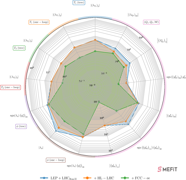
Figure 5.2: The 95% CL upper bounds on the UV-invariant couplings of representative models obtained from the SMEFiT3.0 dataset (blue) and from its extension with the HL-LHC (orange) and with both the HL-LHC and FCC-ee (green) projections. We consider a 3-particle model, $\left(Q_{1},Q_{7},\mathcal{W}\right)$, matched at tree level, and three one-particle models, $T_{1}$, $T_{2}$, and $\phi$, matched at one loop. For the multi-particle model, we set the masses $m_{Q_{1}}=3$ TeV, $m_{Q_{7}}=4.5$ TeV, and $m_{\mathcal{W}}=2.5$ TeV. The one-particle extensions matched at one-loop assume a heavy particle mass of $M_{T_{1}}=M_{T_{2}}=10$ TeV and $M_{\phi}=5$ TeV, representing the indirect mass reach to be probed at the FCC-ee, and for completeness, the associated results from tree-level matching are also displayed.

Consistently with Fig. 5.1, the sensitivity to the heavy fermions $T_{1}$ and $T_{2}$ is not improved at the HL-LHC due to being driven by the constraints from LEP data. Instead, the bounds on these models are significantly tightened after adding the FCC-ee projections. The inclusion of one-loop matching results does not alter this picture and has a small and generally positive impact on the bounds. One-loop matching effects are more marked for the $\phi$ heavy scalar model, where it allows one to constrain the additional UV parameter $|\lambda_{\phi}|$ in all scenarios and with remarkable improvements both at HL-LHC and FCC-ee. The bounds on $|\lambda_{\phi}|$ at LHC Run II and HL-LHC are, however, of limited use since they are beyond the perturbative limit, $|\lambda_{\phi}|<4\pi$. The power of precision measurements at FCC-ee is enough to bring down this bound to a strongly-coupled but perturbative regime, thus providing meaningful information on the UV model. The bound on sgn$(\lambda_{\phi})\left(y_{\phi}^{u}\right)_{33}$ is improved at future colliders for tree-level matching by around $15\%$ at each stage, though the logarithmic scale in the plot hides this improvement. The difference diminishes when considering one-loop matching results and in all cases the bound is within the perturbative limit.

Finally, the results of the multiparticle model display several interesting features. The UV couplings of the heavy fermions, $|(\lambda_{Q_{7}})_{33}|$ and $|(\lambda_{Q_{1}}^{u})_{3}|$, receive improved bounds at both HL-LHC and FCC-ee, as expected since they are related to the coefficients $c_{t\varphi}$ and $c_{\varphi t}$ that show a similar behavior. The UV invariants from the couplings of the heavy spin-1 vector boson with leptons, $|(g_{\mathcal{W}}^{\ell})_{11}|$ and $\text{sgn}((g_{\mathcal{W}}^{\ell})_{11})(g_{\mathcal{W}}^{\ell})_{22}$, see little to no improvement on their bounds from adding HL-LHC projections, but the bounds become at least one order of magnitude tighter once FCC-ee data is considered. A similar situation is found for $\text{sgn}((g_{\mathcal{W}}^{q})_{33})g_{\mathcal{W}}^{\varphi}$, whose bound is driven mostly by its contribution to $c_{\varphi\square}$ and $c_{\varphi\ell_{1}}^{(3)}$ but also affected by its appearance in $c_{\varphi Q}^{(-)}$, $c_{\varphi Q}^{(3)}$ and $c_{b\varphi}$. The UV coupling $g_{\mathcal{W}}^{\varphi}$ also contributes at tree level to $c_{t\varphi}$, which connects the fermionic and bosonic sectors in this model. Such interplay worsens the bound on $\text{sgn}((g_{\mathcal{W}}^{q})_{33})g_{\mathcal{W}}^{\varphi}$ by $\sim 30\%$, which highlights the importance of considering models more complex than the one-particle extensions. The bound on $|(g_{\mathcal{W}}^{q})_{33}|$ is obtained via the Wilson coefficients of four-heavy quark operators such as $c_{QQ}^{1}$ and $c_{QQ}^{8}$. Hence, it improves by around $20\%$ when going from LHC to HL-LHC but is not improved further at future lepton colliders.

6 Summary and outlook

In this work we have quantified the impact that measurements at future colliders, first the HL-LHC and then the FCC-ee and the CEPC, would have on the parameter space of the SMEFT in the framework of a global interpretation of particle physics data. The baseline for these projection studies has been an updated global SMEFT analyses, SMEFiT3.0, combining the constraints from the EWPOs from LEP and SLD with those provided by the recent LHC Run II measurements on Higgs boson, top quark, and diboson production, in many cases based on the full integrated luminosity.

Our analysis provides bounds on $n_{\rm eft}=50$ independent Wilson coefficients (45 in the linear fits) associated to dimension-six operators, with EFT cross-sections being evaluated either at $\mathcal{O}\left(\Lambda^{-2}\right)$ or $\mathcal{O}\left(\Lambda^{-4}\right)$ and including NLO QCD corrections whenever possible. These results are enabled by exploiting newly developed functionalities of the SMEFiT framework, in particular the availability of a projection module which can extrapolate from existing measurements and project them to the settings relevant for other (future) experiments. This module also makes it possible to carry out global SMEFT analyses based on pseudo-data generated with an arbitrary underlying law.

We find that the marginalised bounds on the EFT coefficients within the global fit are projected to improve between around 20% and a factor 3 by the end of the HL-LHC, depending on the operator, with possible further improvements being enabled by optimised analyses not considered here. Subsequently, the constraints from the FCC-ee or the CEPC would markedly improve the bounds on most of the purely bosonic and two-fermion operators entering the fit, by up to two orders of magnitude in some cases. We have then determined, using the UV matching procedure, how this impact at the EFT coefficient level translates into the parameter space of representative one-particle and multi-particle extensions of the SM matched to the SMEFT. We find that the stringent constraints on the interactions of the Higgs, $W$ and $Z$ bosons, and top quarks made possible by future $e^{+}e^{-}$ circular colliders lead to an indirect mass reach on heavy new particles ranging between a few TeV up to around 100 TeV (for UV couplings $g_{\rm UV}\simeq 1$), depending on the specific UV scenario. It is hence clear that the precision FCC-ee/CEPC measurements would make possible an extensive indirect exploration of the landscape of UV models containing new heavy particles beyond the direct reach of HL-LHC.

This work could be extended in several directions. To begin with, we could consider projections for other proposed future colliders, from the ILC and CLIC to the muon collider at different center-of-mass energies, to assess what are their strengths and weaknesses as compared to the FCC-ee and the CEPC in the context of a global SMEFT analysis and its matching to UV models. Second, it would be interesting to further explore whether the EFT impact of Higgs and fermion-pair production at leptonic colliders can be enhanced by including differential information, on the same footing as how it is done for the optimal observables for diboson and top-quark pair production. Third, one may want to include optimised HL-LHC projections, fully exploiting the increase in statistics in ways which cannot be extrapolated from available Run II measurements, such as extended range in differential distributions or finer binning. We expect these to improve the constraints set by HL-LHC on both the SMEFT parameter space and that of the UV-complete models.

Fourth, by extending the analysis of the UV-complete scenarios studied here to other models, both at tree level and via one-loop matching, and in particular considering more general multi-particle models, one could further scrutinise the indirect constraints that quantum corrections on FCC-ee observables impose on the masses and couplings of new heavy particles beyond the reach of the HL-LHC. Fifth, albeit on a longer timescale, one may want to generalise the flavour assumptions on the EFT operators entering the global fit baseline and include data from other processes such as Drell-Yan and $B$-meson decays, and subsequently verify the robustness of the obtained projections for future colliders. In this context, we note that the FCC-ee will also function as a flavour factory, with huge statistics thanks to the large $B$-mesons sample produced in the $Z$-pole run. Finally, the impact of renormalisation group equation running and mixing of the operators would need to be considered to ensure more robust bound setting in global fits such as the one we perform here, where a variety of observables with different energy scales are combined.

As the global particle physics community moves closer to identifying the next large scientific infrastructure projects that will inform the field for the coming decades, the availability of methodologies quantifying the physics reach of different colliders represents an essential tool to make informed decisions. The results of this work demonstrate that the SMEFiT open-source framework is suitable to contribute to this endeavor. Within this framework, progress in the global EFT interpretation of the most updated measurements can be kept synchronised with projections for future colliders, in a way that the baseline always represents the state-of-the-art in terms of experimental constraints. For these reasons, we expect that projections based on SMEFiT will provide a valuable contribution to the upcoming ESPPU and related community studies to take place in the coming few years.

Acknowledgments

We are grateful to M. Bakker for collaboration in initial stages of this work. We acknowledge useful discussions with R. Balasubramanian, J. de Blas, I. Brivio, G. Durieux, C. Grojean, F. Maltoni, K. Mimasu, V. Miralles, C. Severi, and M. Vos. The work of E. C., A. R., M. T. and E. V. is supported by the European Research Council (ERC) under the European Union’s Horizon 2020 research and innovation programme (Grant agreement No. 949451) and by a Royal Society University Research Fellowship through grant URF/R1/201553. The work of L. M. is supported by the European Research Council under the European Union’s Horizon 2020 research and innovation Programme (grant agreement n.950246). The work of J. t. H. and T. G. is supported by the Dutch Research Council (NWO). The work of J. R. is supported by the Dutch Research Council (NWO) and by the Netherlands eScience Center.

Appendix A Fit input settings

Table A.1 collects the overview of the input settings adopted for the SMEFT fits presented in this work. For each fit, we indicate its dataset, whether the EFT coefficients are extracted from a global fit and then marginalised or instead from one parameter individual fits, whether we use actual data or SM pseudo-data, and the treatment of EWPOs (exact versus approximate). In the last column, we list the figures and tables in Sects. 3 and 4 of the paper where the corresponding results are displayed. For all fits listed in this overview, variants at both $\mathcal{O}\left(\Lambda^{-2}\right)$ and $\mathcal{O}\left(\Lambda^{-4}\right)$ in the EFT expansion have been produced.

Dataset	EFT coefficients	Pseudodata?	EWPOs	Figs. & Tables
SMEFiT3.0	Global (Marginalised)	No	Exact	Figs. 3.1, 3.2, 3.3, 3.6, 3.7, Tables 3.3, 3.4
SMEFiT3.0	Individual (one-param)	No	Exact	Table 3.4
SMEFiT2.0	Global (Marginalised)	No	Exact	Fig. 3.7
SMEFiT3.0	Global (Marginalised)	No	Approx.	Fig. 3.6
SMEFiT3.0	Global (Marginalised)	Yes	Exact	Figs. 3.8, 3.9
SMEFiT3.0 + HL-LHC	Global (Marginalised)	Yes	Exact	Figs. 3.8, 3.9
SMEFiT3.0 + HL-LHC	Individual (one-param)	Yes	Exact	Figs. 3.8, 3.9
SMEFiT3.0 + HL-LHC + FCC-ee	Global (Marginalised)	Yes	Exact	Figs. 4.1, 4.2, 4.3, 4.4, 4.5
SMEFiT3.0 + HL-LHC + CEPC	Global (Marginalised)	Yes	Exact	Fig. 4.5

Table A.1: Overview of the input settings used in the fits presented in this work. For each fit, we indicate its dataset, whether the EFT coefficients are extracted from a global fit and then marginalised or instead from one parameter individual fits, whether we use actual data or instead SM pseudo-data is generated, and the treatment of EWPOs (exact versus approximate). In the last column we list the figures and tables in Sects. 3 and 4 of the paper where the corresponding results are displayed. For all fits, variants at both $\mathcal{O}\left(\Lambda^{-2}\right)$ and $\mathcal{O}\left(\Lambda^{-4}\right)$ in the EFT expansion have been produced. The HL-LHC dataset is constructed following the projection described in App. D.

Appendix B SMEFT operator basis

For completeness, we summarise here the SMEFT operator basis and the corresponding flavour assumptions entering this analysis. This basis was first defined in Hartland:2019bjb and then extended in Ethier:2021bye , see also Giani:2023gfq ; terHoeve:2023pvs . It is based on the Warsaw basis of dimension-six operators Grzadkowski:2010es along with a U$(2)_{q}\times$U$(3)_{d}\times$U$(2)_{u}\times(\text{U}(1)_{\ell}\times\text{U}(1)_{e})^{3}$ flavour assumption.

The purely bosonic operators are listed in Table B.1, and the two-fermion and four-lepton operators are defined in Table B.2 and B.3. The four-fermion operators involving bottom and top quarks that we consider are defined in terms of the following Warsaw basis operators:

$$\mathcal{O}_{qq}^{1(ijkl)} =(\bar{q}_{i}\gamma^{\mu}q_{j})(\bar{q}_{k}\gamma_{\mu}q_{l}),$$

$$\mathcal{O}_{qq}^{3(ijkl)} =(\bar{q}_{i}\gamma^{\mu}\tau^{I}q_{j})(\bar{q}_{k}\gamma_{\mu}\tau^{I}q_{l}),$$

$$\mathcal{O}_{qu}^{1(ijkl)} =(\bar{q}_{i}\gamma^{\mu}q_{j})(\bar{u}_{k}\gamma_{\mu}u_{l}),$$

$$\mathcal{O}_{qu}^{8(ijkl)} =(\bar{q}_{i}\gamma^{\mu}T^{A}q_{j})(\bar{u}_{k}\gamma_{\mu}T^{A}u_{l}),$$

$$\mathcal{O}_{qd}^{1(ijkl)} =(\bar{q}_{i}\gamma^{\mu}q_{j})(\bar{d}_{k}\gamma_{\mu}d_{l}),$$

$$\mathcal{O}_{qd}^{8(ijkl)} =(\bar{q}_{i}\gamma^{\mu}T^{A}q_{j})(\bar{d}_{k}\gamma_{\mu}T^{A}d_{l}),$$ (B.1)

$$\mathcal{O}_{uu}^{(ijkl)} =(\bar{u}_{i}\gamma^{\mu}u_{j})(\bar{u}_{k}\gamma_{\mu}u_{l}),$$

$$\mathcal{O}_{ud}^{1(ijkl)} =(\bar{u}_{i}\gamma^{\mu}u_{j})(\bar{d}_{k}\gamma_{\mu}d_{l}),$$

$$\mathcal{O}_{ud}^{8(ijkl)} =(\bar{u}_{i}\gamma^{\mu}T^{A}u_{j})(\bar{d}_{k}\gamma_{\mu}T^{A}d_{l})\,,$$

Then the four-fermion coefficients that enter the fit are linear combinations of the Wilson coefficients of the above operators and are defined in Table B.4. In Eq. (B.1), the left-handed quark doublets are denoted by $q_{i}$ for the first two generations and by $Q$ for the third generation, while $t$ denotes a right-handed top-quark field and $u_{i},d_{i}$ the right-handed $u,c$ and $d,s,b$ fields respectively. The letters $i,j,k,l$ represent the fermion generation indices. All the quarks are considered to be massless except for the top quark. Regarding the leptons, $e,\mu,\tau$ stand for the right-handed charged leptons and $\ell_{i}$ refers to the left-handed leptonic doublets with $i=1,2,3$.

In the conventions that this analysis adopts, the Higgs doublet is indicated by $\varphi$ with vacuum expectation value $v/\sqrt{2}$. We define

$$\varphi^{\dagger}\overset{\text{\scriptsize$\leftrightarrow$}}{D}_{\mu}\,\varphi\equiv\varphi^{\dagger}D_{\mu}\varphi-(D_{\mu}\varphi)^{\dagger}\varphi\ ,\qquad\varphi^{\dagger}\overset{\text{\scriptsize$\leftrightarrow$}}{D}_{\mu}\,\tau_{I}\,\varphi\equiv\varphi^{\dagger}\,\tau_{I}D_{\mu}\varphi-(D_{\mu}\varphi)^{\dagger}\tau_{I}\varphi\,,$$ (B.2)

where the covariant derivative is given by:

$$D_{\mu}\varphi=\Big{(}\partial_{\mu}-i\frac{g}{2}\tau_{I}W_{\mu}^{I}-i\frac{g^{\prime}}{2}B_{\mu}\Big{)}\varphi\,.$$ (B.3)

Here $W_{\mu},\,B_{\mu}$ are the electroweak gauge bosons fields, $g$ and $g^{\prime}$ are the $SU(2)_{L}$ and $U(1)_{Y}$ couplings respectively and $\tau_{I}$ are the Pauli sigma matrices. Furthermore $G^{A}_{\mu\nu}$, $W^{\mu\nu}$ and $B^{\mu\nu}$ stand for the $SU(3)_{C}$, $SU(2)_{L}$ and $U(1)_{Y}$ field strength tensors. $T^{A}=\frac{1}{2}\lambda^{A}$ are the $SU(3)$ generators where $\lambda^{A}$ are the Gell-Mann matrices. The strong coupling constant is denoted by $g_{s}$, $\theta$ represents the weak mixing angle, and $\tau^{\mu\nu}=\frac{1}{2}[\gamma^{\mu},\gamma^{\nu}]$.

Operator	Coefficient	Definition	Operator	Coefficient	Definition
$\mathcal{O}_{\scriptscriptstyle\varphi G}$	$c_{\varphi G}$	$\left(\varphi^{\dagger}\varphi\right)G^{\mu\nu}_{\scriptscriptstyle A}\,G_{\mu\nu}^{\scriptscriptstyle A}$	$\mathcal{O}_{\scriptscriptstyle\varphi\square}$	$c_{\varphi\square}$	$\partial_{\mu}(\varphi^{\dagger}\varphi)\partial^{\mu}(\varphi^{\dagger}\varphi)$
$\mathcal{O}_{\scriptscriptstyle\varphi B}$	$c_{\varphi B}$	$\left(\varphi^{\dagger}\varphi\right)B^{\mu\nu}\,B_{\mu\nu}$	$\mathcal{O}_{\scriptscriptstyle\varphi D}$	$c_{\varphi D}$	$(\varphi^{\dagger}D^{\mu}\varphi)^{\dagger}(\varphi^{\dagger}D_{\mu}\varphi)$
$\mathcal{O}_{\scriptscriptstyle\varphi W}$	$c_{\varphi W}$	$\left(\varphi^{\dagger}\varphi\right)W^{\mu\nu}_{\scriptscriptstyle I}\,W_{\mu\nu}^{\scriptscriptstyle I}$	$\mathcal{O}_{W}$	$c_{WWW}$	$\epsilon_{IJK}W_{\mu\nu}^{I}W^{J,\nu\rho}W^{K,\mu}_{\rho}$
$\mathcal{O}_{\scriptscriptstyle\varphi WB}$	$c_{\varphi WB}$	$(\varphi^{\dagger}\tau_{\scriptscriptstyle I}\varphi)\,B^{\mu\nu}W_{\mu\nu}^{\scriptscriptstyle I}\,$

Table B.1: Purely bosonic dimension-six operators that modify the production and decay of Higgs bosons and the interactions of the electroweak gauge bosons. For each operator, we indicate its definition in terms of the SM fields, and the conventions that are used both for the operator and for the coefficient. See Ethier:2021bye for more details.

Operator	Coefficient	Definition	Operator	Coefficient	Definition
3rd generation quarks
$\mathcal{O}_{\scriptscriptstyle\varphi Q}^{(1)}$	$c_{\varphi Q}^{(1)}$ (*)	$i\big{(}\varphi^{\dagger}\overset{\text{\scriptsize$\leftrightarrow$}}{D}_{\mu}\,\varphi\big{)}\big{(}\bar{Q}\,\gamma^{\mu}\,Q\big{)}$	$\mathcal{O}_{\scriptscriptstyle tW}$	$c_{tW}$	$i\big{(}\bar{Q}\tau^{\mu\nu}\,\tau_{\scriptscriptstyle I}\,t\big{)}\,\tilde{\varphi}\,W^{I}_{\mu\nu}+\text{h.c.}$
$\mathcal{O}_{\scriptscriptstyle\varphi Q}^{(3)}$	$c_{\varphi Q}^{(3)}$	$i\big{(}\varphi^{\dagger}\overset{\text{\scriptsize$\leftrightarrow$}}{D}_{\mu}\,\tau_{\scriptscriptstyle I}\varphi\big{)}\big{(}\bar{Q}\,\gamma^{\mu}\,\tau^{\scriptscriptstyle I}Q\big{)}$	$\mathcal{O}_{\scriptscriptstyle tB}$	$c_{tB}$ (*)	$i\big{(}\bar{Q}\tau^{\mu\nu}\,t\big{)}\,\tilde{\varphi}\,B_{\mu\nu}+\text{h.c.}$
$\mathcal{O}_{\scriptscriptstyle\varphi t}$	$c_{\varphi t}$	$i\big{(}\varphi^{\dagger}\,\overset{\text{\scriptsize$\leftrightarrow$}}{D}_{\mu}\,\,\varphi\big{)}\big{(}\bar{t}\,\gamma^{\mu}\,t\big{)}$	$\mathcal{O}_{\scriptscriptstyle tG}$	$c_{tG}$	$ig{\scriptscriptstyle S}\,\big{(}\bar{Q}\tau^{\mu\nu}\,T_{\scriptscriptstyle A}\,t\big{)}\,\tilde{\varphi}\,G^{A}_{\mu\nu}+\text{h.c.}$
$\mathcal{O}_{\scriptscriptstyle t\varphi}$	$c_{t\varphi}$	$\left(\varphi^{\dagger}\varphi\right)\bar{Q}\,t\,\tilde{\varphi}+\text{h.c.}$	$\mathcal{O}_{\scriptscriptstyle b\varphi}$	$c_{b\varphi}$	$\left(\varphi^{\dagger}\varphi\right)\bar{Q}\,b\,\varphi+\text{h.c.}$
1st, 2nd generation quarks
$\mathcal{O}_{\scriptscriptstyle\varphi q}^{(1)}$	$c_{\varphi q}^{(1)}$ (*)	$\sum\limits_{\scriptscriptstyle i=1,2}i\big{(}\varphi^{\dagger}\overset{\text{\scriptsize$\leftrightarrow$}}{D}_{\mu}\,\varphi\big{)}\big{(}\bar{q}_{i}\,\gamma^{\mu}\,q_{i}\big{)}$	${\mathcal{O}_{\scriptscriptstyle\varphi d}}$	${{c_{\varphi d}}}$	$\sum\limits_{\scriptscriptstyle i=1,2,3}i\big{(}\varphi^{\dagger}\,\overset{\text{\scriptsize$\leftrightarrow$}}{D}_{\mu}\,\,\varphi\big{)}\big{(}\bar{d}_{i}\,\gamma^{\mu}\,d_{i}\big{)}$
$\mathcal{O}_{\scriptscriptstyle\varphi q}^{(3)}$	$c_{\varphi q}^{(3)}$	$\sum\limits_{\scriptscriptstyle i=1,2}i\big{(}\varphi^{\dagger}\overset{\text{\scriptsize$\leftrightarrow$}}{D}_{\mu}\,\tau_{\scriptscriptstyle I}\varphi\big{)}\big{(}\bar{q}_{i}\,\gamma^{\mu}\,\tau^{\scriptscriptstyle I}q_{i}\big{)}$	$\mathcal{O}_{\scriptscriptstyle c\varphi}$	$c_{c\varphi}$	$\left(\varphi^{\dagger}\varphi\right)\bar{q}_{2}\,c\,\tilde{\varphi}+\text{h.c.}$
${\mathcal{O}_{\scriptscriptstyle\varphi u}}$	${{c_{\varphi u}}}$	$\sum\limits_{\scriptscriptstyle i=1,2}i\big{(}\varphi^{\dagger}\,\overset{\text{\scriptsize$\leftrightarrow$}}{D}_{\mu}\,\,\varphi\big{)}\big{(}\bar{u}_{i}\,\gamma^{\mu}\,u_{i}\big{)}$
two-leptons
$\mathcal{O}_{\scriptscriptstyle\varphi\ell_{i}}$	$c_{\varphi\ell_{i}}$	$i\big{(}\varphi^{\dagger}\overset{\text{\scriptsize$\leftrightarrow$}}{D}_{\mu}\,\varphi\big{)}\big{(}\bar{\ell}_{i}\,\gamma^{\mu}\,\ell_{i}\big{)}$	$\mathcal{O}_{\scriptscriptstyle\varphi\mu}$	$c_{\varphi\mu}$	$i\big{(}\varphi^{\dagger}\overset{\text{\scriptsize$\leftrightarrow$}}{D}_{\mu}\,\varphi\big{)}\big{(}\bar{\mu}\,\gamma^{\mu}\,\mu\big{)}$
$\mathcal{O}_{\scriptscriptstyle\varphi\ell_{i}}^{(3)}$	$c_{\varphi\ell_{i}}^{(3)}$	$i\big{(}\varphi^{\dagger}\overset{\text{\scriptsize$\leftrightarrow$}}{D}_{\mu}\,\tau_{\scriptscriptstyle I}\varphi\big{)}\big{(}\bar{\ell}_{i}\,\gamma^{\mu}\,\tau^{\scriptscriptstyle I}\ell_{i}\big{)}$	$\mathcal{O}_{\scriptscriptstyle\varphi\tau}$	$c_{\varphi\tau}$	$i\big{(}\varphi^{\dagger}\overset{\text{\scriptsize$\leftrightarrow$}}{D}_{\mu}\,\varphi\big{)}\big{(}\bar{\tau}\,\gamma^{\mu}\,\tau\big{)}$
$\mathcal{O}_{\scriptscriptstyle\varphi e}$	$c_{\varphi e}$	$i\big{(}\varphi^{\dagger}\overset{\text{\scriptsize$\leftrightarrow$}}{D}_{\mu}\,\varphi\big{)}\big{(}\bar{e}\,\gamma^{\mu}\,e\big{)}$	$\mathcal{O}_{\scriptscriptstyle\tau\varphi}$	$c_{\tau\varphi}$	$\left(\varphi^{\dagger}\varphi\right)\bar{\ell_{3}}\,\tau\,{\varphi}+\text{h.c.}$
four-leptons
$\mathcal{O}_{\scriptscriptstyle\ell\ell}$	$c_{\ell\ell}$	$\left(\bar{\ell}_{1}\gamma_{\mu}\ell_{2}\right)\left(\bar{\ell}_{2}\gamma^{\mu}\ell_{1}\right)$

Table B.2: Same as Table B.1 for the operators containing two fermion fields, either quarks or leptons, as well as the four-lepton operator $\mathcal{O}_{\scriptscriptstyle\ell\ell}$. The flavour index $i$ runs from 1 to 3. The coefficients indicated with (*) in the second column do not correspond to physical degrees of freedom in the fit, but are rather replaced by $c_{\varphi q}^{(-)}$, $c_{\varphi Q}^{(-)}$, and $c_{tZ}$ defined in Table B.3.

Coefficient	Definition
$c_{\varphi Q}^{(-)}$	$c_{\varphi Q}^{(1)}-c_{\varphi Q}^{(3)}$
$c_{tZ}$	$-s_{\theta}\,c_{tB}+c_{\theta}\,c_{tW}$
$c_{\varphi q}^{(-)}$	$c_{\varphi q}^{(1)}-c_{\varphi q}^{(3)}$

Table B.3: Linear combinations of two-fermion operators listed in Table B.2 and that enter at the fit level instead of those marked with (*).

DoF	Definition (in Warsaw basis notation)	DoF	Definition (in Warsaw basis notation)
$c_{QQ}^{1}$	$2c_{qq}^{1(3333)}-\frac{2}{3}c_{qq}^{3(3333)}$	$c_{QQ}^{8}$	$8c_{qq}^{3(3333)}$
$c_{Qt}^{1}$	$c_{qu}^{1(3333)}$	$c_{Qt}^{8}$	$c_{qu}^{8(3333)}$
$c_{Qq}^{1,8}$	$c_{qq}^{1(i33i)}+3c_{qq}^{3(i33i)}$	$c_{Qq}^{1,1}$	$c_{qq}^{1(ii33)}+\frac{1}{6}c_{qq}^{1(i33i)}+\frac{1}{2}c_{qq}^{3(i33i)}$
$c_{Qq}^{3,8}$	$c_{qq}^{1(i33i)}-c_{qq}^{3(i33i)}$	$c_{Qq}^{3,1}$	$c_{qq}^{3(ii33)}+\frac{1}{6}(c_{qq}^{1(i33i)}-c_{qq}^{3(i33i)})$
$c_{tq}^{8}$	$c_{qu}^{8(ii33)}$	$c_{tq}^{1}$	$c_{qu}^{1(ii33)}$
$c_{tu}^{8}$	$2c_{uu}^{(i33i)}$	$c_{tu}^{1}$	$c_{uu}^{(ii33)}+\frac{1}{3}c_{uu}^{(i33i)}$
$c_{Qu}^{8}$	$c_{qu}^{8(33ii)}$	$c_{Qu}^{1}$	$c_{qu}^{1(33ii)}$
$c_{td}^{8}$	$c_{ud}^{8(33jj)}$	$c_{td}^{1}$	$c_{ud}^{1(33jj)}$
$c_{Qd}^{8}$	$c_{qd}^{8(33jj)}$	$c_{Qd}^{1}$	$c_{qd}^{1(33jj)}$

Table B.4: Definition of the four-fermion coefficients that enter in the fit in terms of the coefficients of Warsaw basis operators of Eq. (B.1). These coefficients are classified into four-heavy (upper part) and two-light-two-heavy (bottom part) operators. The flavour index $i$ is either 1 or 2, and $j$ is either 1, 2 or 3: with our flavour assumptions, these coefficients will be the same regardless of the specific values that $i$ and $j$ take.

Appendix C EWPOs implementation: benchmarking and validation

Our implementation of EWPOs in SMEFiT, described in Sect. 2, has been cross-checked and validated with previous studies, in particular with the analysis of Brivio:2017bnu . To highlight the consistency of our implementation with previous results, we provide in Fig. C.1 a comparison of single parameter fits at linear order in the EFT carried out with SMEFiT with the EWPO data in Table 2.1 against the corresponding analysis from Brivio:2017bnu based on the same dataset and assuming flavour universality for comparison purposes. The triple gauge operator $O_{WWW}$ differs from the SMEFT@NLO convention by a minus sign to adopt the same conventions as Brivio:2017bnu , and has been fitted to the same subset of the available LEP data on $WW$ production composed of only 4 bins. Excellent agreement is found for all operators, further validating the implementation of EWPOs presented in this work.

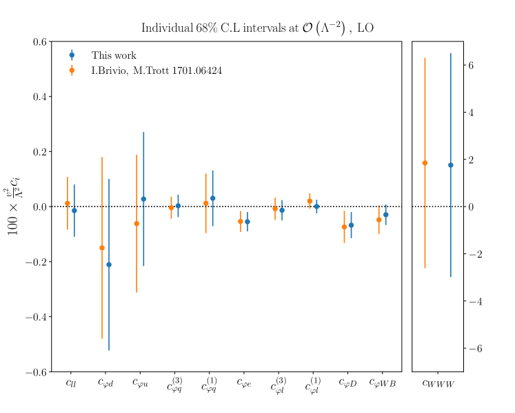
Figure C.1: Comparison of a SMEFiT-based analysis of the EWPOs from LEP against the corresponding analysis from Brivio:2017bnu . We display bounds at the $68\%$ CL for one-parameter fits using linear EFT and LO calculations. One should note that we adopt the convention of Brivio:2017bnu for the triple gauge operator $O_{WWW}$, which differs from the SMEFT@NLO one by a negative sign. For consistency with the settings adopted in Brivio:2017bnu , the triple gauge operator coefficient $c_{WWW}$ has been fitted to a subset of the available LEP data on diboson production composed by only 4 bins.

Appendix D Projections for the HL-LHC

Incorporating projections from future $e^{+}e^{-}$ collider measurements into a global SMEFT analysis based on currently available data (LHC Run II with full luminosity) may provide an overly optimistic picture of their impact in the EFT parameter space, given that HL-LHC program will have already yielded constraints for these operators. Any impact study for future colliders therefore needs to build upon a realistic baseline quantifying the constraints on the SMEFT coefficients which will have been achieved by the end of the “guaranteed” HL-LHC running operations.

Here we describe the procedure that we have adopted in order to extrapolate existing LHC Run II measurements to the HL-LHC conditions. These projections are used to quantify the impact of Higgs, top quark, and diboson production measurements at the HL-LHC on the SMEFT parameter space, and the corresponding results have been presented in Sect. 3.3. These projections assume the SM as the underlying theory. We note that dedicated projections for HL-LHC pseudo-data are available e.g. deBlas:2019rxi ; deBlas:2022ofj ; DeBlas:2019qco ; Durieux:2022cvf and references therein. Here we adopt instead a different strategy to ensure consistency with the SMEFiT analysis settings, based on generating pseudo-data for future LHC runs by means of extrapolating from available Run II datasets.

To this end, we use a new SMEFiT module generating projections of pseudo-data for future experiments. This projection is based on extrapolating existing datasets, acquired at the same center-of-mass energy but lower luminosities, for the same underlying process. The same strategy was adopted in Ethier:2021ydt ; Greljo:2021kvv for the SMEFT impact projections of vector-boson scattering and high-mass Drell-Yan data at the HL-LHC, as well as in the PDF projections at the HL-LHC AbdulKhalek:2018rok and at the Forward Physics Facility of Cruz-Martinez:2023sdv ; Feng:2022inv .

This module starts by considering a given available measurement from the LHC Run II, composed by $n_{\rm bin}$ data points, and with the corresponding SM predictions given by $\mathcal{O}_{i}^{{\rm(th)}}$. The central values for the pseudo-data, denoted by $\mathcal{O}_{i}^{{\rm(exp)}}$, are obtained by fluctuating these theory predictions by the fractional statistical ($\delta_{i}^{\rm(stat)}$) and systematic ($\delta_{k,i}^{\rm(sys)}$) uncertainties,

$$\mathcal{O}_{i}^{{\rm(exp)}}=\mathcal{O}_{i}^{{\rm(th)}}\left(1+r_{i}\delta_{i}^{\rm(stat)}+\sum_{k=1}^{n_{\rm sys}}r_{k,i}\delta_{k,i}^{\rm(sys)}\right)\,,\qquad i=1,\ldots,n_{\rm bin}\,,$$ (D.1)

where $r_{i}$ and $r_{k,i}$ are univariate random Gaussian numbers, whose distribution is such as to reproduce the experimental covariance matrix of the data, and the index $k$ runs over the individual sources of correlated systematic errors. We note that theory uncertainties are not included in the pseudo-data generation, and enter only the calculation of the $\chi^{2}$.

Since one is extrapolating from an existing measurement, whose associated statistical and systematic errors are denoted by $\tilde{\delta}_{i}^{\rm(stat)}$ and $\tilde{\delta}_{k,i}^{\rm(sys)}$, one needs to account for the increased statistics and the expected reduction of the systematic uncertainties for the HL-LHC data-taking period. The former follows from the increase in integrated luminosity,

$$\delta_{i}^{\rm(stat)}=\tilde{\delta}_{i}^{\rm(stat)}\sqrt{\frac{\mathcal{L}_{\rm Run2}}{\mathcal{L}_{\rm HLLHC}}}\,,\qquad i=1,\ldots,n_{\rm bin}\,,$$ (D.2)

while the reduction of systematic errors is estimated by means of an overall rescaling factor

$$\delta_{k,i}^{\rm(sys)}=\tilde{\delta}_{k,i}^{\rm(sys)}\times f_{\rm red}^{(k)}\,,\qquad i=1,\ldots,n_{\rm bin}\,,\quad k=1,\ldots,n_{\rm sys}\,.$$ (D.3)

with $f_{\rm red}^{(k)}$ indicating a correction estimating improvements in the experimental performance, in many cases possible thanks to the larger available event sample. Here for simplicity we adopt the optimistic scenario considered in the HL-LHC projection studies Cepeda:2019klc , namely $f_{\rm red}^{(k)}=1/2$ for all the datasets. For datasets without the breakdown of statistical and systematic errors, Eq. (D.1) is replaced by

$$\mathcal{O}_{i}^{{\rm(exp)}}=\mathcal{O}_{i}^{{\rm(th)}}\left(1+r_{i}\delta_{i}^{\rm(tot)}\right)\,,\qquad i=1,\ldots,n_{\rm bin}\,,$$ (D.4)

with the total error being reduced by a factor $\delta_{i}^{\rm(tot)}=f_{\rm red}^{{\rm tot}}\times\tilde{\delta}_{i}^{\rm(tot)}$ with $f_{\rm red}^{{\rm tot}}\sim 1/3$, namely the average of the expected reduction of statistical and systematic uncertainties as compared to the baseline Run II measurements. For such datasets, the correlations are neglected in the projections due to the lack of their breakdown.

The main benefit of our approach is the possibility to extrapolate the full set of processes entering the current SMEFT global fit, to make sure that all relevant directions in the parameter space are covered in these projections, as well as bypassing the need to evaluate separately the SM and SMEFT theory predictions. One drawback is that it does not account for the possible increase in kinematic range covered by HL-LHC measurements, for example with additional bins in the high-energy region, which can only be considered on a case-by-case basis.

Tables D.1 and D.2 provide the overview of the LHC Run II datasets on Higgs, top quark, and diboson production datasets that are adopted as input for the projections at the HL-LHC. For each dataset, we specify the corresponding internal SMEFiT label, the total integrated luminosity, the final state and physical observable, the number of data points and the publication reference. We only project datasets that are both part of SMEFiT3.0, as described in Sect. 3, and which are based on the highest integrated luminosity for a given process type. Note that for each process type and final state one can include at most two different projections, given that both ATLAS and CMS will perform independent measurements in the HL-LHC data-taking period.

When generating pseudo-data based on some known underlying law, the total $\chi^{2}$ values will depend on the random seed used for the pseudo-data generation. Statistical consistency of the procedure demands that the empirical distribution of these $\chi^{2}$ values over a large number of different sets of synthetic pseudo-data follows a $\chi^{2}$ distribution with the appropriate number of degrees of freedom. This expectation is for instance explicitly verified in the Level-1 closure tests carried out in the context of the NNPDF proton structure analyses NNPDF:2021njg ; NNPDF:2014otw ; DelDebbio:2021whr .

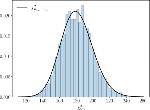
Figure D.1: Histogram displaying the distribution of the total $\chi^{2}_{\rm tot}$ values obtained by repeatedly drawing independent HL-LHC pseudo-datasets following the prescription specified in Eq. D.1 and then carrying out the corresponding SMEFT analysis at $\mathcal{O}\left(\Lambda^{-2}\right)$ in the EFT expansion. The black curve corresponds to the $\chi^{2}$ distribution associated to fitting $n_{{\rm dat}}$ data points with $n_{{\rm eft}}$ Wilson coefficients. Good agreement between the two distributions is found, demonstrating the statistical consistency of the HL-LHC pseudo-data generation.

To verify this property in the present analysis, Fig. D.1 displays the histogram with the empirical distribution of the total $\chi^{2}$ values obtained by repeatedly drawing independent HL-LHC pseudo-datasets, following the prescription specified in this appendix and then carrying out the corresponding SMEFT analysis at linear order in the EFT expansion. The black curve corresponds to the theoretical $\chi^{2}$ expectation associated to fitting $n_{\rm dat}$ data points with $n_{\rm eft}$ Wilson coefficients. Excellent agreement between the two distributions is found, demonstrating the statistical consistency of pseudo-data generation procedure in the SMEFiT projection module.

Dataset	$\mathcal{L}$ $\left(\rm{fb}^{-1}\right)$	Info	Observables	$n_{\rm dat}$	Ref.
ATLAS_STXS_RunII_13TeV_2022	139	$gg$F, VBF, $Vh$, $t\bar{t}h$, $th$	$d\sigma/dp_{T}^{h}$	36	ATLAS:2022vkf
			$d\sigma/dm_{jj}$
			$d\sigma/dp_{T}^{V}$
CMS_ggF_aa_13TeV	$77.4$	$gg$F, $h\rightarrow\gamma\gamma$	$\sigma_{gg\rm{F}}(p_{T}^{h},N_{\rm jets})$	6	CMS:2019xnv
ATLAS_ggF_ZZ_13TeV	$79.8$	$gg$F, $h\rightarrow ZZ$	$\sigma_{gg\rm{F}}(p_{T}^{h},N_{\rm jets})$	6	ATLAS:2019nkf
ATLAS_ggF_13TeV_2015	$36.1$	$gg$F, $h\rightarrow ZZ,h\rightarrow\gamma\gamma$	$d\sigma(gg\mathrm{F})/dp_{T}^{h}$	9	ATLAS:2018pgp
ATLAS_WH_Hbb_13TeV	$79.8$	$Wh,h\rightarrow b\bar{b}$	$d\sigma^{(\rm fid)}/dp_{T}^{W}$ (stage 1 STXS)	2	ATLAS:2019yhn
ATLAS_ZH_Hbb_13TeV	$79.8$	$Zh,h\rightarrow b\bar{b}$	$d\sigma^{(\rm fid)}/dp_{T}^{Z}$ (stage 1 STXS)	2	ATLAS:2019yhn
CMS_H_13TeV_2015_pTH	$35.9$	$h\rightarrow b\bar{b},h\rightarrow\gamma\gamma,h\rightarrow ZZ$	$d\sigma/dp_{T}^{h}$	9	CMS:2018gwt
ATLAS_WW_13TeV_2016_memu	$36.1$	fully leptonic	$d\sigma^{(\mathrm{fid})}/dm_{e\mu}$	13	ATLAS:2019rob
ATLAS_WZ_13TeV_2016_mTWZ	$36.1$	fully leptonic	$d\sigma^{(\mathrm{fid})}/dm_{T}^{WZ}$	6	ATLAS:2019bsc
CMS_WZ_13TeV_2016_pTZ	$35.9$	fully leptonic	$d\sigma^{(\mathrm{fid})}/dp_{T}^{Z}$	11	CMS:2019efc
CMS_WZ_13TeV_2022_pTZ	$137$	fully leptonic	$d\sigma/dp_{T}^{Z}$	11	CMS:2021icx

Table D.1: LHC Run II datasets for Higgs and diboson production ($\sqrt{s}=13$ TeV) used as input to the HL-LHC extrapolations. For each dataset, we indicate its internal SMEFiT label together with its integrated luminosity $\mathcal{L}$ (in $\rm{fb}^{-1}$), the final state or the specific production mechanism, the physical observable, the number of data points, and the corresponding publication reference. We only project datasets that are part of SMEFiT3.0, which are selected on the basis of the highest integrated luminosity for each process type.

Dataset	$\mathcal{L}$ $\left(\rm{fb}^{-1}\right)$	Info	Observables	$n_{\rm dat}$	Ref.
ATLAS_tt_13TeV_ljets_2016_Mtt	$36.1$	$\ell$+jets	$d\sigma/dm_{t\bar{t}}$	7	ATLAS:2019hxz
CMS_tt_13TeV_dilep_2016_Mtt	$35.9$	dilepton	$d\sigma/dm_{t\bar{t}}$	7	CMS:2018adi
CMS_tt_13TeV_Mtt	$137$	$\ell$+jets	$1/\sigma d\sigma/dm_{t\bar{t}}$	14	CMS:2021vhb
CMS_tt_13TeV_ljets_inc	$137$	$\ell$+jets	$\sigma(t\bar{t})$	1	CMS:2021vhb
ATLAS_tt_13TeV_asy_2022	$139$	$\ell$ + jets	$A_{C}$	5	ATLAS:2022waa
CMS_tt_13TeV_asy	$138$	$\ell$ + jets	$A_{C}$	3	CMS:2022ged
ATLAS_Whel_13TeV	139	$W$-helicity fraction	$F_{0},F_{L}$	2	ATLAS:2022rms
ATLAS_ttbb_13TeV_2016	$36.1$	lepton + jets	$\sigma_{\rm tot}(t\bar{t}b\bar{b})$	1	ATLAS:2018fwl
CMS_ttbb_13TeV_2016	$35.9$	all-jets	$\sigma_{\rm tot}(t\bar{t}b\bar{b})$	1	CMS:2019eih
CMS_ttbb_13TeV_dilepton_inc	$35.9$	dilepton	$\sigma_{\rm tot}(t\bar{t}b\bar{b})$	1	CMS:2020grm
CMS_ttbb_13TeV_ljets_inc	$35.9$	lepton + jets	$\sigma_{\rm tot}(t\bar{t}b\bar{b})$	1	CMS:2020grm
ATLAS_tttt_13TeV_run2	$139$	multi-lepton	$\sigma_{\rm tot}(t\bar{t}t\bar{t})$	1	ATLAS:2020hpj
CMS_tttt_13TeV_run2	$137$	same-sign or multi-lepton	$\sigma_{\rm tot}(t\bar{t}t\bar{t})$	1	CMS:2019rvj
ATLAS_tttt_13TeV_slep_inc	$139$	single-lepton	$\sigma_{\rm tot}(t\bar{t}t\bar{t})$	1	ATLAS:2021kqb
CMS_tttt_13TeV_slep_inc	$35.8$	single-lepton	$\sigma_{\rm tot}(t\bar{t}t\bar{t})$	1	CMS:2019jsc
ATLAS_tttt_13TeV_2023	$139$	multi-lepton	$\sigma_{\rm tot}(t\bar{t}t\bar{t})$	1	ATLAS:2023ajo
CMS_tttt_13TeV_2023	$139$	same-sign or multi-lepton	$\sigma_{\rm tot}(t\bar{t}t\bar{t})$	1	CMS:2023ftu
CMS_ttZ_13TeV_pTZ	$77.5$	$t\bar{t}Z$	$d\sigma(t\bar{t}Z)/dp_{T}^{Z}$	4	CMS:2019too
ATLAS_ttZ_13TeV_pTZ	$139$	$t\bar{t}Z$	$d\sigma(t\bar{t}Z)/dp_{T}^{Z}$	7	ATLAS:2021fzm
ATLAS_ttW_13TeV_2016	$36.1$	$t\bar{t}W$	$\sigma_{\mathrm{tot}}(t\bar{t}W)$	1	ATLAS:2019fwo
CMS_ttW_13TeV	$35.9$	$t\bar{t}W$	$\sigma_{\mathrm{tot}}(t\bar{t}W)$	1	CMS:2017ugv
ATLAS_t_tch_13TeV_inc	$3.2$	$t$-channel	$\sigma_{\mathrm{tot}}(tq),\sigma_{\mathrm{tot}}(\bar{t}q)$	2	ATLAS:2016qhd
CMS_t_tch_13TeV_2019_diff_Yt	$35.9$	$t$-channel	$d\sigma/d|y_{t}|$	5	CMS:2019jjp
ATLAS_t_sch_13TeV_inc	$139$	$s$-channel	$\sigma(t+\bar{t})$	1	ATLAS:2022wfk
ATLAS_tW_13TeV_inc	$3.2$	multi-lepton	$\sigma_{\mathrm{tot}}(tW)$	1	ATLAS:2016ofl
CMS_tW_13TeV_inc	$35.9$	multi-lepton	$\sigma_{\mathrm{tot}}(tW)$	1	CMS:2018amb
CMS_tW_13TeV_slep_inc	$36$	single-lepton	$\sigma_{\mathrm{tot}}(tW)$	1	CMS:2021vqm
ATLAS_tZ_13TeV_run2_inc	$139$	multi-lepton + jets	$\sigma_{\rm fid}(t\ell^{+}\ell^{-}q)$	1	ATLAS:2020bhu
CMS_tZ_13TeV_pTt	138	multi-lepton + jets	$d\sigma_{\rm fid}(tZj)/dp_{T}^{t}$	3	CMS:2021ugv

Table D.2: Same as Table D.1 for processes involving top quark production.

By analogy with the terminology adopted in the NNPDF closure test analyses, here we denote projections based on fluctuating the pseudo-data around the associated theory predictions, Eqns. (D.1) and (D.4), as ‘Level-1’ projections. This is the baseline strategy used in the EFT projections presented in this paper, and corresponds to the expected sensitivity obtained from the analysis of the actual data in the case of perfect compatibility with the SM theory predictions. An alternative strategy, which corresponds to what is done in other projection studies, corresponds to fitting without fluctuating the pseudo-data, namely

$$\mathcal{O}_{i}^{{\rm(exp)}}=\mathcal{O}_{i}^{{\rm(th)}}\,,\qquad i=1,\ldots,n_{\rm bin}\,,$$ (D.5)

instead of Eqns. (D.1) and (D.4). We denote projections based on Eq. (D.5) as ‘Level-0’ projections. These are now independent of the random seed used for the pseudo-data generation and result in a post-fit value of $\chi^{2}\simeq 0$, but may be overly optimistic since they miss the layer of statistical fluctuations which accompanies any real measurement.

We have assessed the impact of HL-LHC and FCC-ee pseudo-data based on either Level-1 or Level-0 projections, finding in general excellent agreement. The only differences arise at the level of the individual fits carried out at the $\mathcal{O}\left(\Lambda^{-4}\right)$ level, where for some coefficients the impact of the pseudo-data becomes somewhat more marked in the Level-0 projections.

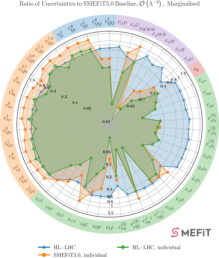
Figure D.2: Same as Fig. 3.9, but now based on Level-0 pseudo-data projections.

This feature is illustrated by Fig. D.2, which provides the same information as the HL-LHC projections of Fig. 3.9 now based on Level-0 pseudo-data.

Comparing pair-wise these two plots, one finds that the sensitivity estimates for the marginalised (quadratic) fits are unchanged, but that some differences are visible for the individual fits. For instance, in the Level-0 projections one can see a clear improvement in the bounds associated to the two-light-two-heavy operators thanks to the HL-LHC pseudo-data, which is not necessarily the case in the corresponding Level-1 projections. Level-0 projections quantifying the impact of the FCC-ee pseudo-data are very similar to the Level-1 ones shown in Fig. 4.3, and hence are not considered here. All in all, differences between Level-1 and Level-0 projections are very moderate and restricted mostly to the two-light-two-heavy and four-heavy operators in the individual quadratic EFT fits with HL-LHC pseudo-data.

Appendix E FCC-ee and CEPC projections: observables and uncertainties

Here we provide the list of observables that are being considered in the SMEFT analyses with FCC-ee or CEPC pseudo-data presented in Sect. 4. We describe only the measurements included at the level of total cross-sections or signal strengths, since differential distributions in $W^{+}W^{-}$ and $t\bar{t}$ production are accounted for by means of the unbinned optimal observables formalism and discussed in App. F. For each process, we also indicate the experimental uncertainties that have been provided by the corresponding experimental collaborations.

To begin with, Table E.1 displays the $Z$-pole ($\sqrt{s}=91.2$ GeV) electroweak precision observables for the FCC-ee and CEPC considered in this analysis, corresponding to the running scenarios of these two colliders described in Sect. 4.1. For each observable, we indicate the expected absolute ($\Delta$) or relative ($\delta$) statistical and experimental systematic uncertainties.

$Z$-pole EWPOs ($\sqrt{s}=91.2$ GeV)
$\qquad\quad\mathcal{O}_{i}$	$\delta/\Delta~{}\mathcal{O}_{i}$
	FCC-ee	CEPC
$\alpha(m_{Z})^{-1}\,(\times 10^{3})$	$\Delta=2.7$ (1.2)	$\Delta=17.8$
$\Gamma_{W}$ (MeV)	$\Delta=0.85$ (0.3)	$\Delta=1.8$ (0.9)
$\Gamma_{Z}$ (MeV)	$\Delta=0.0028$ (0.025)	$\Delta=0.005$ (0.025)
$A_{e}\,(\times 10^{5})$	$\Delta=0.5$ (2)	$\Delta=1.5$
$A_{\mu}\,(\times 10^{5})$	$\Delta=1.6$ (2.2)	$\Delta=3.0~{}(1.8)$
$A_{\tau}\,(\times 10^{5})$	$\Delta=0.35$ (20)	$\Delta=1.2~{}(6.9)$
$A_{b}\,(\times 10^{5})$	$\Delta=1.7$ (21)	$\Delta=3~{}(21)$
$A_{c}\,(\times 10^{5})$	$\Delta=14$ (15)	$\Delta=6~{}(30)$
$\sigma_{\text{had}}^{0}$ (pb)	$\Delta=0.025~{}(4)$	$\Delta=0.05~{}(2)$
$R_{e}\,(\times 10^{3})$	$\delta=0.0028$ (0.3)	$\delta=0.003~{}(0.2)$
$R_{\mu}\,(\times 10^{3})$	$\delta=0.0021$ (0.05)	$\delta=0.003~{}(0.1)$
$R_{\tau}\,(\times 10^{3})$	$\delta=0.0021$ (0.1)	$\delta=0.003~{}(0.1)$
$R_{b}\,(\times 10^{3})$	$\delta=0.001$ (0.3)	$\delta=0.005~{}(0.2)$
$R_{c}\,(\times 10^{3})$	$\delta=0.011$ (1.5)	$\delta=0.02$ (1)

Table E.1: The $Z$-pole ($\sqrt{s}=91.2$ GeV) electroweak precision observables for the FCC-ee and CEPC considered in this analysis, corresponding to the running scenarios described in Sect. 4.1. For each observable, we indicate the expected statistical (systematic) experimental uncertainty, either in absolute units ($\Delta$) or relative to the central value ($\delta$). See Sect. 2 for the definitions of these observables.

Then Table E.2 provides analogous information to Table E.1 for light fermion pair production at $\sqrt{s}=240$ and 365 GeV. For each of the di-fermion final states considered ($e^{+}e^{-}$, $\mu^{+}\mu^{-}$, $\tau^{+}\tau^{-}$, $c\bar{c}$, and $b\bar{b}$), we indicate the absolute uncertainty both for the total cross-section and for the forward-backward asymmetry. For each final state we assume a total selection efficiency of 0.98, 0.98, 0.9, 0.03 and 0.15 respectively, and an acceptance angle around the beam corresponding to $|\cos(\theta)|=0.9,0.95,0.9,0.9,0.9$, for all energies and collider scenarios. The central values are assumed to correspond to the SM predictions, as for all the other observables considered in this work.

$e^{+}e^{-}\to f\bar{f}$
	$\sqrt{s}=240$ GeV		$\sqrt{s}=365$ GeV
$\qquad\quad\mathcal{O}_{i}$	$\Delta_{\exp}\mathcal{O}_{i}$ (FCC-ee)	$\Delta_{\exp}\mathcal{O}_{i}$ (CEPC)	$\Delta_{\exp}\mathcal{O}_{i}$ (FCC-ee)	$\Delta_{\exp}\mathcal{O}_{i}$ (CEPC)
$\sigma_{\rm tot}(e^{+}e^{-})$ [fb]	2.29	1.62	2.74	4.68
$A_{\rm FB}(e^{+}e^{-})$	$9.79\cdot 10^{-6}$	$6.92\cdot 10^{-6}$	$2.83\cdot 10^{-5}$	$4.83\cdot 10^{-5}$
$\sigma_{\rm tot}(\mu^{+}\mu^{-})$ [fb]	0.405	0.287	0.48	0.82
$A_{\rm FB}(\mu^{+}\mu^{-})$	$1.98\cdot 10^{-4}$	$1.397\cdot 10^{-4}$	$5.69\cdot 10^{-4}$	$9.7\cdot 10^{-4}$
$\sigma_{\rm tot}(\tau^{+}\tau^{-})$ [fb]	0.374	0.264	0.443	0.756
$A_{\rm FB}(\tau^{+}\tau^{-})$	$2.17\cdot 10^{-4}$	$1.53\cdot 10^{-4}$	$6.24\cdot 10^{-4}$	0.00106
$\sigma_{\rm tot}(c\bar{c})$ [fb]	0.088	0.062	0.102	0.175
$A_{\rm FB}(c\bar{c})$	0.000813	$5.74\cdot 10^{-4}$	0.00238	0.00405
$\sigma_{\rm tot}(b\bar{b})$ [fb]	0.151	0.107	0.171	0.29
$A_{\rm FB}(b\bar{b})$	$4.86\cdot 10^{-4}$	$3.44\cdot 10^{-4}$	0.00142	0.00243

Table E.2: Same as Table E.1 for light-fermion pair production at $\sqrt{s}=240$ and 365 GeV. For each of the di-fermion final states considered, we indicate the absolute statistical uncertainty both for the total cross-section and for the forward-backward asymmetry $A_{\rm FB}$ defined in Eq. (2.35). As for all projections considered in this work, the corresponding central values are set to be equal to the SM predictions.

We list the projections for Higgs production measurements at the FCC-ee and the CEPC in Table E.3. We display the forecast relative experimental uncertainties for the inclusive production cross-section in the $Zh$ channel, $\sigma_{Zh}$, and for the corresponding Higgs signal strengths (production times decay) at $\sqrt{s}=240$ and 365 GeV, for different final states, for both the associated production ($Zh$) and vector-boson fusion ($h\nu\nu$) channels. The final states considered are $b\bar{b}$, $c\bar{c}$, $gg$, $ZZ$, $WW$, $\tau^{+}\tau^{-}$, $\gamma Z$ and $\gamma\gamma$. For the $\sqrt{s}=240$ data-taking period, only the $b\bar{b}$ final state is available in the vector-boson fusion production channel.

$e^{+}e^{-}\to Zh$
	$\sqrt{s}=240$ GeV		$\sqrt{s}=365$ GeV
$\mathcal{O}_{i}$	$\delta_{\exp}\mathcal{O}_{i}$ (FCC-ee)	$\delta_{\exp}\mathcal{O}_{i}$ (CEPC)	$\delta_{\exp}\mathcal{O}_{i}$ (FCC-ee)	$\delta_{\exp}\mathcal{O}_{i}$ (CEPC)
$\sigma_{Zh}$	0.0035	0.0026	0.0064	0.014
$\sigma_{Zh}\times{\rm BR}_{b\bar{b}}$	0.0021	0.0014	0.0035	0.009
$\sigma_{Zh}\times{\rm BR}_{c\bar{c}}$	0.0156	0.0202	0.046	0.088
$\sigma_{Zh}\times{\rm BR}_{gg}$	0.0134	0.0081	0.0247	0.034
$\sigma_{Zh}\times{\rm BR}_{ZZ}$	0.0311	0.0417	0.0849	0.2
$\sigma_{Zh}\times{\rm BR}_{WW}$	0.0085	0.0053	0.0184	0.028
$\sigma_{Zh}\times{\rm BR}_{\tau^{+}\tau^{-}}$	0.0064	0.0042	0.0127	0.021
$\sigma_{Zh}\times{\rm BR}_{\gamma\gamma}$	0.0636	0.0302	0.127	0.11
$\sigma_{Zh}\times{\rm BR}_{\gamma Z}$	0.12	0.085	-	-
$e^{+}e^{-}\to h\nu\nu$
	$\sqrt{s}=240$ GeV		$\sqrt{s}=365$ GeV
$\mathcal{O}_{i}$	$\delta_{\exp}\mathcal{O}_{i}$ (FCC-ee)	$\delta_{\exp}\mathcal{O}_{i}$ (CEPC)	$\delta_{\exp}\mathcal{O}_{i}$ (FCC-ee)	$\delta_{\exp}\mathcal{O}_{i}$ (CEPC)
$\sigma_{h\nu\nu}\times{\rm BR}_{b\bar{b}}$	0.0219	0.0159	0.0064	0.011
$\sigma_{h\nu\nu}\times{\rm BR}_{c\bar{c}}$	-	-	0.0707	0.16
$\sigma_{h\nu\nu}\times{\rm BR}_{gg}$	-	-	0.0318	0.045
$\sigma_{h\nu\nu}\times{\rm BR}_{ZZ}$	-	-	0.0707	0.21
$\sigma_{h\nu\nu}\times{\rm BR}_{WW}$	-	-	0.0255	0.044
$\sigma_{h\nu\nu}\times{\rm BR}_{\tau^{+}\tau^{-}}$	-	-	0.0566	0.042
$\sigma_{h\nu\nu}\times{\rm BR}_{\gamma\gamma}$	-	-	0.156	0.16

Table E.3: Same as Table E.1 for the relative statistical experimental uncertainties projected for the inclusive production cross-section in the $Zh$ channel, $\sigma_{Zh}$, and for the corresponding Higgs signal strengths (production times decay) at $\sqrt{s}=240$ and 365 GeV, for different final states. The signal strengths are provided for both the associated production ($Zh$) and the vector-boson fusion ($h\nu\nu$) channels. The corresponding central values are taken from the SM predictions.

Finally, we also consider in our analysis the inclusive cross section of $W^{+}W^{-}$ production and the individual leptonic $W$ branching ratios. We indicate in Table E.4 the forecast relative uncertainties for these observables at FCC-ee and CEPC for the three relevant center of mass energies: $\sqrt{s}=161$ GeV, 240 GeV, and 365 GeV. The leptonic branching ratio uncertainty is assumed to be the same for each of the three lepton generations, while the uncertainty associated to hadronic $W$ decays is constrained from enforcing the lack of exotic decays, i.e. Eq. 4.3. The uncertainties listed in Table E.4 for the FCC-ee were extracted from DeBlas:2019qco , and in the case of CEPC were rescaled by the appropriate luminosity factors to match with its baseline running scenario. We note that the measurements indicated in Table E.4 do not overlap with the optimal observables from $W^{+}W^{-}$ production described in App. F, since the latter are normalised and implemented at the level of undecayed $W$ bosons.

$e^{+}e^{-}\to W^{+}W^{-}$
$\mathcal{O}_{i}$	$\sqrt{s}=161$ GeV		$\sqrt{s}=240$ GeV		$\sqrt{s}=365$ GeV
	$\delta_{\exp}$ (FCC-ee)	$\delta_{\exp}$ (CEPC)	$\delta_{\exp}$ (FCC-ee)	$\delta_{\exp}$ (CEPC)	$\delta_{\exp}$ (FCC-ee)	$\delta_{\exp}$ (CEPC)
$\sigma_{WW}$	$1.36\cdot 10^{-4}$	$2.48\cdot 10^{-4}$	$1.22\cdot 10^{-4}$	$8.63\cdot 10^{-5}$	$2.81\cdot 10^{-4}$	$4.87\cdot 10^{-4}$
BR${}_{W\to\ell_{i}\nu_{i}}$	$2.72\cdot 10^{-4}$	$4.95\cdot 10^{-4}$	$2.44\cdot 10^{-4}$	$1.73\cdot 10^{-4}$	$5.63\cdot 10^{-4}$	$9.75\cdot 10^{-4}$

Table E.4: Same as Table E.1 for the relative experimental uncertainties associated to the measurements of the inclusive $e^{+}e^{-}\to W^{+}W^{-}$ cross section and the leptonic $W$ branching ratio at FCC-ee and CEPC. The leptonic branching fraction measurements are considered separately for the three generations.

To summarise, for the projections of both FCC-ee and CEPC, we consider the $Z$-pole EWPOs, fermion pair production at $\sqrt{s}=240$ GeV and $365$ GeV, $W^{+}W^{-}$ production (including branching fractions) at $\sqrt{s}=161$ GeV, $240$ GeV and $365$ GeV, and Higgs production and decay in various final states (including signal strengths) at $\sqrt{s}=240$ GeV and $365$ GeV. Furthermore, we also include the optimal observables for normalised differential distributions in diboson and top-quark pair production, as discussed in App. F.

Appendix F Optimal observables at future lepton colliders

For processes well described by linear EFT corrections, with negligible systematic uncertainties, and where the kinematic information is available on an event-by-event basis, one can use the technique of “optimal observables” Diehl:1993br . This technique maximizes the sensitivity to the EFT coefficients by exploiting the information contained in the fully differential cross-section. In this work, the projected differential measurements of both $W^{+}W^{-}$ and $t\bar{t}$ production at FCC-ee and CEPC are included in terms of such optimal observables in the same manner as in DeBlas:2019qco ; deBlas:2022ofj . In this appendix we summarize our treatment of these observables in the global SMEFT analysis, keeping the discussion fully general.

Optimal observable definition.

For physical observables characterised by a linear dependence on $n_{\rm eft}$ EFT coefficients, the fully differential distribution can be expressed as

$$\frac{\rm d\sigma_{\rm th}}{\rm d\Phi}=\left(S_{\rm SM}(\Phi)+\sum_{k=1}^{n_{\rm eft}}c_{k}S_{k}(\Phi)\right)\equiv S(\Phi)\,,$$ (F.1)

where $\Phi$ represents the final-state kinematic variables, $S_{\rm SM}(\Phi)$ is the SM squared matrix element (including phase space factors) and $S_{k}(\Phi)$ the corresponding linear (interference) EFT matrix element. Eq. (F.1) assumes that quadratic EFT corrections and beyond can be neglected, and factors of $\Lambda^{-2}$ have been reabsorbed in the Wilson coefficient $c_{k}$. These observables may be extended to the case of quadratic EFT corrections via Machine Learning techniques Chen:2020mev ; GomezAmbrosio:2022mpm ; Chen:2023ind , but we have verified that keeping only the linear piece is a good approximation for the processes we consider here.

We consider now an experiment that measures $n_{\rm ev}$ events, each one characterised by their own set of kinematic final-state variables, ${\Phi_{1},...,\Phi_{n_{\rm ev}}}$, such as rapidities and transverse momenta. Depending on the type of measurement, $\Phi_{i}$ could represent parton-level, particle-level, or detector-level variables. The optimal observables are constructed on an event-by-event basis as

$$\mathcal{O}^{(\rm exp)}_{k,i}=\frac{S_{k}(\Phi_{i})}{S_{\rm SM}(\Phi_{i})}\equiv\frac{S_{k,i}}{S_{{\rm SM},i}}\,,\quad i=1,\ldots,n_{\rm ev}\,,\quad k=1,\ldots,n_{\rm eft}\,,$$ (F.2)

that is, as the ratio between the linear EFT and the SM matrix elements, evaluated at the kinematics of the corresponding event $\Phi_{i}$. The expectation value of these observables is then obtained by averaging over the full set of events, namely

$$\left\langle\mathcal{O}^{(\rm exp)}_{k}\right\rangle=\frac{1}{n_{\rm ev}}\sum_{i=1}^{n_{\rm ev}}\frac{S_{k}(\Phi_{i})}{S_{\rm SM}(\Phi_{i})}\equiv\frac{1}{n_{\rm ev}}\sum_{i=1}^{n_{\rm ev}}\frac{S_{k,i}}{S_{{\rm SM},i}}\,,\qquad k=1,\ldots,n_{\rm eft}\,,$$ (F.3)

separately for each of the relevant Wilson coefficients. For a given integrated luminosity $\mathcal{L}$ and fiducial (SM) cross-section $\sigma_{\rm SM}$, the total number of events $n_{\rm ev}$ follows a Poisson distribution with mean $\lambda=n_{\rm ev}=\mathcal{L}\,\sigma_{\rm SM}$, where we neglect effects such as acceptances and efficiencies. In the following, we assume for simplicity that $n_{\rm ev}$ corresponds to the mean value of this distribution.

Theoretical predictions for the expectation value of the optimal observables defined in Eq. (F.3) can be evaluated either analytically or numerically, depending on the complexity of the calculation. Here, since we are making projections for future colliders, we assume that the measured experimental values agree with the SM theoretical prediction. As explained below, this allows us to rotate both the observables and the inverse covariance matrix in a basis such that the rotated observables coincide with the Wilson coefficients, $\widetilde{\mathcal{O}}_{k}=c_{k}$. Expressed in this basis, the inverse experimental covariance matrix takes the simple form Diehl:1993br ; DeBlas:2019qco ,

$$\left({\rm cov}_{\rm exp}\left(c_{k},c_{k^{\prime}}\right)\right)^{-1}=\mathcal{L}\left(\int\frac{S_{k}\,S_{k^{\prime}}}{S_{\rm SM}}\,{\rm d\Phi}-\frac{1}{\sigma_{\rm SM}}\int S_{k}{\rm d\Phi}\int S_{k^{\prime}}{\rm d\Phi}\right).$$ (F.4)

For relatively simple processes, the phase space integrals in Eq. (F.4) can be computed analytically. The final contribution to the global fit figure of merit arising from these optimal observables is then

$$\Delta\chi^{2}\left({\bm{c}}\right)=\sum_{k,k^{\prime}=1}^{n_{\rm eft}}c_{k}\left({\rm cov}_{\rm exp}\left(c_{k},c_{k^{\prime}}\right)\right)^{-1}c_{k^{\prime}}\,,$$ (F.5)

where, since we assume the SM, in the rotated basis the experimental values for the Wilson coefficients vanish.

Observable rotation.

The evaluation of the contribution to the total $\chi^{2}$ from the optimal observables is performed most efficiently in a rotated basis, where these observables are matched to each one of the individual Wilson coefficients entering the theory prediction. Let one assume that we have a set of $N$ observables that depend linearly on $n_{\rm eft}$ EFT coefficients, that is,

$$\sigma^{(i)}_{\rm th}=\sigma^{(i)}_{\rm SM}+\sum_{k=1}^{n_{\rm eft}}\sigma^{(i)}_{k}c_{k}\,,\quad\quad i=1,...,N\,,$$ (F.6)

where $\sigma^{(i)}_{k}$ is the linear EFT cross-section, and again factors of $\Lambda^{-2}$ are reabsorbed in the Wilson coefficient. For simplicity, we assume that the measured values of these $N$ observables coincide with the corresponding SM prediction, $\sigma^{(i)}_{\text{exp}}=\sigma^{(i)}_{\rm SM}$. Furthermore, the $N$ observables are distributed according to a multi-Gaussian likelihood. In this case, we can express the contribution of these $N$ observables to the figure of merit of the global EFT fit as follows

$$\Delta\chi^{2} =\sum_{i,j=1}^{N}\left(\sigma^{(i)}_{\rm exp}-\sigma^{(i)}_{\rm th}\right)\left(\text{cov}_{\rm exp}\right)^{-1}_{ij}\left(\sigma^{(j)}_{\rm exp}-\sigma^{(j)}_{\rm th}\right)$$

$$=\sum_{i,j=1}^{N}\left(\sum_{k=1}^{n_{\rm eft}}\sigma^{(i)}_{k}c_{k}\right)\left(\text{cov}_{\rm exp}\right)^{-1}_{ij}\left(\sum_{k^{\prime}=1}^{n_{\rm eft}}\sigma^{(j)}_{k^{\prime}}c_{k^{\prime}}\right)\,,$$ (F.7)

where $\left(\text{cov}_{\rm exp}\right)_{ij}$ is the experimental covariance matrix between the observables $\sigma^{(i)}_{\text{exp}}$ and $\sigma^{(j)}_{\text{exp}}$. If the measured quantities did not agree with their SM predictions, the following steps could still be performed after adding and subtracting the mean of the Wilson coefficients and with an additional constant term in $\Delta\chi^{2}$.

One can rewrite Eq. (F.7) in a more compact manner as follows:

$$\Delta\chi^{2}=\sum_{k,k^{\prime}=1}^{n_{\rm eft}}c_{k}c_{k^{\prime}}\sum_{i,j=1}^{N}\sigma^{(i)}_{k}\left(\text{cov}_{\rm exp}\right)^{-1}_{ij}\sigma^{(j)}_{k^{\prime}}\equiv\sum_{k,k^{\prime}=1}^{n_{\rm eft}}c_{k}A^{\sigma}_{kk^{\prime}}c_{k^{\prime}}\,,$$ (F.8)

in terms of a new covariance matrix, now in the space of Wilson coefficients, defined as

$$A^{\sigma}_{kk^{\prime}}=\sum_{i,j=1}^{N}\sigma^{(i)}_{k}\left(\text{cov}_{\rm exp}\right)^{-1}_{ij}\sigma^{(j)}_{k^{\prime}}\,,\qquad k,k^{\prime}=1,\ldots,n_{\rm eft}\,,$$ (F.9)

and obtained by multiplying the linear EFT cross-sections with the inverse of the experimental covariance matrix. The result of Eq. (F.9) indicates that one can define new observables in terms of individual Wilson coefficients,

$$\widetilde{\sigma}^{(k)}=c_{k}\,,\qquad k=1,\ldots,n_{\rm eft}\,,$$ (F.10)

with $A^{\sigma}_{kk^{\prime}}$ as inverse covariance matrix, that is

$${\rm cov}_{\rm exp}\left(\widetilde{\sigma}^{(k)},\widetilde{\sigma}^{(k^{\prime})}\right)^{-1}=A^{\sigma}_{kk^{\prime}}\,.$$ (F.11)

Note that the original covariance matrix $\left(\text{cov}_{\rm exp}\right)_{ij}$ lives in the space $N\times N$ spanned by the experimental data, while the covariance matrix for the redefined observables, ${\rm cov}_{\rm exp}\left(\widetilde{\sigma}^{(k)},\widetilde{\sigma}^{(k^{\prime})}\right)$, instead lives in the $n_{\rm eft}\times n_{\rm eft}$ space spanned by the Wilson coefficients. This transformation is only possible when EFT corrections beyond the linear correction are neglected.

The main advantage of this redefinition is that one can easily evaluate the covariance matrix $A^{\sigma}_{kk^{\prime}}$, in the scenario where the observables are statistically limited. Then, Eq. (F.9) accounts for them in the global fit, as has been done in Eq. (F.5) above.

Implementation.

The optimal observable framework reviewed in this appendix is used to include in the fit the FCC-ee and CEPC projections for differential distributions in $W^{+}W^{-}$ and $t\bar{t}$ production.

In the case of $W^{+}W^{-}$ production, we consider measurements taken from the $\sqrt{s}=161$ GeV ($W$ pair-production threshold), $240$ GeV and $365$ GeV data-taking periods, each one for the integrated luminosities indicated in Table 4.1. We include the fully leptonic and semi-leptonic $W$ decay channels and treat on the same footing the three lepton generations. We assume that the experiment will be able to measure the momenta of all the final state fermions by assuming on-shell $W$s, i.e. a perfect neutrino reconstruction. However, we account for the inability to distinguish the quarks produced by a hadronic $W$ decay by implementing the corresponding angle-folding effect. Furthermore, we assume an overall signal selection efficiency of $45\%$ and a detector acceptance cut on the polar angle of $|\cos\theta|<0.9$ and $0.95$ for jets and leptons respectively, in agreement with previous studies DeBlas:2019qco ; deBlas:2022ofj . The selection efficiency is implemented by rescaling the luminosity while the acceptance cuts determine the phase-space region over which we integrate. We computed the inverse covariance matrix by performing the required phase space integrals by suitably modifying the phase-space integrator included in MadGraph5. We validated our results against a method based on the reweighting of LHE events like the one used in Durieux:2018tev .

$W^{+}W^{-}$ production at $e^{+}e^{-}$ colliders is in principle sensitive to eight of the dimension-six operators considered in the SMEFiT global analysis, namely

$$\mathcal{O}_{\varphi D},\,\mathcal{O}_{\varphi WB},\,\mathcal{O}_{WWW},\,\mathcal{O}_{\varphi\ell_{1}},\,\,\mathcal{O}_{\varphi e},\,\mathcal{O}_{\varphi\ell_{1}}^{(3)},\,\mathcal{O}_{\varphi\ell_{2}}^{(3)},\,\mathcal{O}_{\ell\ell}\,.$$ (F.12)

However, the linear combination of coefficients $c_{\varphi\ell_{1}}^{(3)}+\,c_{\varphi\ell_{2}}^{(3)}-2c_{\ell\ell}$ only modifies the inclusive cross-section via input parameters shifts, to which the optimal observables defined with normalized differential distributions are insensitive. Moreover, the coefficients $c_{\varphi\ell_{2}}^{(3)}$ and $c_{\ell\ell}$ enter only through the previous linear combination and $c_{\varphi\ell_{1}}^{(3)}$ modifies on its own the $eeZ$ and $e\nu_{e}W$ interaction vertices. These considerations indicate that the optimal observables considered here have associated two flat directions, which we remove from the inverse covariance before the fit. All in all, the (normalized) optimal observables in $W^{+}W^{-}$ production at FCC-ee/CEPC constrain six EFT coefficients:

$$c_{\varphi D},\,c_{\varphi{WB}},\,c_{WWW},\,c_{\varphi\ell_{1}},\,\,c_{\varphi e},\,c_{\varphi\ell_{1}}^{(3)},$$ (F.13)

in agreement with previous studies DeBlas:2019qco ; deBlas:2022ofj .

In the case of top-quark pair production, we took the inverse covariance matrix defining the optimal observables from the Snowmass study deBlas:2022ofj , used there for the HEPfit interpretation of future collider projections. These optimal observables are non-zero only for $\sqrt{s}=365$ GeV, just above the top pair production threshold. While for $W^{+}W^{-}$ we used the definition for normalized differential distributions, Eq. (F.4), for $t\bar{t}$ we use optimal observables that include the information in the inclusive cross-section, which equates to considering only the first term on the right-hand side of Eq. (F.4). They offer sensitivity to eight CP-even dimension-six operators, four of which are semi-leptonic four-fermion operators. Since the latter are not included in the SMEFiT global fit, we neglect them. Hence, the projections for $e^{+}e^{-}\to t\bar{t}$ measurements at the FCC-ee and the CEPC constrain the following coefficients

$$c_{\varphi Q}^{(-)},\,c_{\varphi t},\,c_{tW},\,c_{tZ}\,,$$ (F.14)

hence providing complementary sensitivity to the LHC measurements of top quark production.

Appendix G SMEFT effects in the $W$-boson decay widths

Here whenever we evaluate theoretical predictions for processes involving the production and decay of $W$ bosons with mg5_aMC@NLO, we assume a constant value of the $W$ boson decay width. However, this fixed-width approximation is theoretically inconsistent, since it neglects the corrections that SMEFT dimension-six operators introduce at the $W$ width level. In this appendix, we describe our approach to account a posteriori for SMEFT effects entering the $W$-boson decay widths, which follows the procedure developed in Brivio:2019myy . We spell out the procedure in the case of $WW$ production in the fully-leptonic channel, i.e. $W\rightarrow\ell\nu$, but the same approach applies to any other process involving $W$ boson decays.

The starting point is to assume that one can factorise production and decay effects in the $WW$ process by writing

$$\sigma_{WW\rightarrow 4\ell}=X^{(\rm th)}f(\Gamma_{W}),$$ (G.1)

with production effects encoded in

$$X^{(\rm th)}=X^{(\rm sm)}+\sum_{j=1}^{n_{\rm eft}}c_{j}X_{j}^{(\rm eft)}+\sum_{j=1}^{n_{\rm eft}}\sum_{k\geq j}^{n_{\rm eft}}c_{j}c_{k}X_{jk}^{(\rm eft)}\,,$$ (G.2)

with $X^{(\rm sm)}$ indicating the SM prediction and $X_{j}^{(\rm eft)}$ and $X_{jk}^{(\rm eft)}$ the linear and quadratic SMEFT corrections respectively for the $n_{\rm eft}$ dimension-six operators relevant for the analysis. Effects related to the $W$-boson widths are then encapsulated in the $f(\Gamma_{W})$ term. In the narrow-width approximation, one has $f(\Gamma_{W})=1/\Gamma_{W}^{2}$ in the case of two decaying $W$s, but the actual dependence on the width is in general more convoluted.

Next, one assumes that SMEFT effects distort the SM value of the $W$-boson width, $\Gamma_{W}^{(\rm sm)}$, by a moderate amount only. This allows us to carry out the following Taylor expansion:

$$f(\Gamma_{W})=f(\Gamma_{W}^{(\rm sm)}+\delta\Gamma_{W})\approx f\left(\Gamma_{W}^{(\rm sm)}\right)\left(1+\delta_{1}\frac{\delta\Gamma_{W}}{\Gamma_{W}^{(\rm sm)}}+\delta_{2}\left(\frac{\delta\Gamma_{W}}{\Gamma_{W}^{(\rm sm)}}\right)^{2}+\mathcal{O}\left(\frac{\delta\Gamma_{W}}{\Gamma_{W}^{(\rm sm)}}\right)^{3}\right),$$ (G.3)

where $\delta\Gamma_{W}$ accounts for SMEFT effects to the decay width, and where terms cubic on $\delta\Gamma_{W}$ and beyond are neglected. Substituting Eqns. (G.2) and (G.3) into Eq. (G.1) results into

$$\sigma_{WW\rightarrow 4\ell} =\left(X^{(\rm sm)}+\sum_{j=1}^{n_{\rm eft}}c_{j}X_{j}^{(\rm eft)}+\sum_{j=1}^{n_{\rm eft}}\sum_{k\geq j}^{n_{\rm eft}}c_{j}c_{k}X_{jk}^{(\rm eft)}\right)f\left(\Gamma_{W}^{(\rm sm)}\right)\left(1+\delta_{1}\frac{\delta\Gamma_{W}}{\Gamma_{W}^{(\rm sm)}}+\delta_{2}\left(\frac{\delta\Gamma_{W}}{\Gamma_{W}^{(\rm sm)}}\right)^{2}\right)$$

$$\equiv\left(\sigma_{WW\rightarrow 4\ell}^{\rm(sm)}+\sum_{j=1}^{n_{\rm eft}}c_{j}Y_{j}^{(\rm eft)}+\sum_{j=1}^{n_{\rm eft}}\sum_{k\geq j}^{n_{\rm eft}}c_{j}c_{k}Y_{jk}^{(\rm eft)}\right)\left(1+\delta_{1}\frac{\delta\Gamma_{W}}{\Gamma_{W}^{(\rm sm)}}+\delta_{2}\left(\frac{\delta\Gamma_{W}}{\Gamma_{W}^{(\rm sm)}}\right)^{2}\right),$$ (G.4)

where we have defined

$$\sigma_{WW\rightarrow 4\ell}^{\rm(sm)}\equiv X^{\rm(sm)}f\left(\Gamma_{W}^{\rm(sm)}\right)\qquad\text{and}\qquad Y_{i}\equiv X_{i}f\left(\Gamma_{W}^{\rm(sm)}\right)\,.$$ (G.5)

Given that we compute the SMEFT corrections to the $WW$ process in the fixed-width approximation (that is, assuming $\delta\Gamma_{W}=0$), we already know the coefficients $Y_{j}^{(\rm eft)}$ and $Y_{jk}^{(\rm eft)}$. What remains to be done is to determine the expansion coefficients $\delta_{1}$ and $\delta_{2}$ in Eq. (G.4). To do so, we evaluate the differential cross-section, $\sigma_{WW\rightarrow 4\ell}$, setting to zero all EFT effects while varying the width $\Gamma_{W}$ along a fixed set of values $\delta\Gamma_{W}^{(i)}=\{\delta\Gamma_{W}^{(1)},\dots,\delta\Gamma_{W}^{(n)}\}$ around the SM corresponding to $\delta\Gamma_{W}=0$. One can then fit a quartic polynomial to the resulting values

$$\sigma_{WW\rightarrow 4\ell}^{(i)}=\sigma_{WW\rightarrow 4\ell}^{\rm(sm)}\left(1+\delta_{1}\frac{\delta\Gamma_{W}^{(i)}}{\Gamma_{W}^{(\rm sm)}}+\delta_{2}\left(\frac{\delta\Gamma_{W}^{(i)}}{\Gamma_{W}^{(\rm sm)}}\right)^{2}+\delta_{3}\left(\frac{\delta\Gamma_{W}^{(i)}}{\Gamma_{W}^{(\rm sm)}}\right)^{3}+\delta_{4}\left(\frac{\delta\Gamma_{W}^{(i)}}{\Gamma_{W}^{(\rm sm)}}\right)^{4}\right)\,,\qquad i=1,\dots,n\,,$$ (G.6)

to extract the expansion coefficients $\delta_{1}$ and $\delta_{2}$. At the level of the polynomial fit, we also include the expansion coefficients $\delta_{3}$ and $\delta_{4}$, which are relevant in case the fitting range extends beyond the quadratic regime where cubic and quartic effects introduce sizeable corrections that would otherwise get absorbed into incorrect values of $\delta_{1}$ and $\delta_{2}$. In the following, we will not write $\delta_{3}$ and $\delta_{4}$ explicitly with the understanding that $\delta_{1}$ and $\delta_{2}$ are always determined in a quartic fit.

The last ingredient required is to compute the shifts $\delta\Gamma_{W}$ in Eq. (G.3) as a function of the SMEFT coefficients in our fitting basis. To this end, we parameterise these shifts as

$$\delta\Gamma_{W}=\sum_{j=1}^{n_{\rm eft}}c_{j}Z_{j}^{(\rm eft)}+\sum_{j=1}^{n_{\rm eft}}\sum_{k\geq j}^{n_{\rm eft}}c_{j}c_{k}Z_{jk}^{(\rm eft)},$$ (G.7)

in terms of the linear and quadratic corrections, and where the coefficients $Z_{j}$ and $Z_{jk}$ can be computed analytically. One then substitutes Eq. (G.7) into Eq. (G.4) and up to quadratic corrections this gives:

$$\sigma_{WW\rightarrow 4\ell}=\left(\sigma_{WW\rightarrow 4\ell}^{\rm(sm)}+\sum_{j=1}^{n_{\rm eft}}c_{j}Y_{j}^{(\rm eft)}+\sum_{j=1}^{n_{\rm eft}}\sum_{k\geq j}^{n_{\rm eft}}c_{j}c_{k}Y_{jk}^{(\rm eft)}\right)$$

$$\qquad\times\left(1+\frac{\delta_{1}}{\Gamma_{W}^{\rm(sm)}}\left(\sum_{j=1}^{n_{\rm eft}}c_{j}Z_{j}^{(\rm eft)}+\sum_{j=1}^{n_{\rm eft}}\sum_{k\geq j}^{n_{\rm eft}}c_{j}c_{k}Z_{jk}^{(\rm eft)}\right)+\frac{\delta_{2}}{\left(\Gamma_{W}^{\rm(sm)}\right)^{2}}\left(\sum_{j=1}^{n_{\rm eft}}c_{j}Z_{j}^{(\rm eft)}\right)^{2}\right)\,,$$ (G.8)

where higher-order terms in the expansion beyond quadratic corrections are neglected. We can now equate terms proportional to the same power of the Wilson coefficients to determine how the SMEFT corrections to production, $Y_{i}^{(\rm eft)}$ and $Y_{ij}^{(\rm eft)}$ in Eq. (G.4), are modified in the presence of corrections to the $W$-boson decay width:

$$\sigma_{WW\rightarrow 4\ell}=\left(\sigma_{WW\rightarrow 4\ell}^{\rm(sm)}+\sum_{j=1}^{n_{\rm eft}}c_{j}\widetilde{Y}_{j}^{(\rm eft)}+\sum_{j=1}^{n_{\rm eft}}\sum_{k\geq j}^{n_{\rm eft}}c_{j}c_{k}\widetilde{Y}_{jk}^{(\rm eft)}\right)\,,$$ (G.9)

with

$$\widetilde{Y}_{i} =Y_{i}^{\rm(eft)}+\frac{\delta_{1}}{\Gamma_{W}^{\rm(sm)}}Z_{i}^{\rm(eft)}\sigma_{WW\rightarrow 4\ell}^{\rm(sm)}\,,$$ (G.10)

$$\widetilde{Y}_{ii}^{\rm(eft)} =Y_{ii}^{\rm(eft)}+\sigma_{WW\rightarrow 4\ell}^{\rm(sm)}\left(\frac{\delta_{1}}{\Gamma_{W}^{\rm(sm)}}Z_{ii}^{\rm(eft)}+\frac{\delta_{2}}{\left(\Gamma_{W}^{\rm(sm)}\right)^{2}}\left(Z_{i}^{\rm(eft)}\right)^{2}\right)+\frac{\delta_{1}}{\Gamma_{W}^{\rm(sm)}}Y_{i}^{\rm(eft)}Z_{i}^{\rm(eft)}\,,$$ (G.11)

$$\widetilde{Y}_{ij}^{\rm(eft)} =Y_{ij}^{\rm(eft)}+\sigma_{WW\rightarrow 4\ell}^{\rm(sm)}\left(\frac{\delta_{1}}{\Gamma_{W}^{\rm(sm)}}Z_{ij}^{\rm(eft)}+2\frac{\delta_{2}}{\left(\Gamma_{W}^{\rm(sm)}\right)^{2}}Z_{i}^{\rm(eft)}Z_{j}^{\rm(eft)}\right)$$

$$\hskip 85.35826pt+\frac{\delta_{1}}{\Gamma_{W}^{\rm(sm)}}\left(Y_{i}^{\rm(eft)}Z_{j}^{\rm(eft)}+Y_{j}^{\rm(eft)}Z_{i}^{\rm(eft)}\right)\,,\qquad i\neq j.$$ (G.12)

Eqns. (G.10)–(G.12) indicate how to account for SMEFT effects in the decay width in the case of theory calculations carried out in the fixed-width approximation.

Multiple widths.

This approach can be generalised to processes depending on multiple decay widths, like $\Gamma_{Z}$ and $\Gamma_{W}$ in $WZ$ production. One should modify Eq. (G.6) to

$$\sigma_{WZ\rightarrow 4\ell} =\sigma_{WZ\rightarrow 4\ell}^{\rm(sm)}\left(1+\delta_{1}^{W}\frac{\delta\Gamma_{W}}{\Gamma_{W}^{(\rm sm)}}+\delta_{2}^{W}\left(\frac{\delta\Gamma_{W}}{\Gamma_{W}^{(\rm sm)}}\right)^{2}+\delta_{1}^{Z}\frac{\delta\Gamma_{Z}}{\Gamma_{Z}^{(\rm sm)}}+\delta_{2}^{Z}\left(\frac{\delta\Gamma_{Z}}{\Gamma_{Z}^{(\rm sm)}}\right)^{2}+\delta^{ZW}\frac{\delta\Gamma_{Z}\delta\Gamma_{W}}{\Gamma_{W}^{(\rm sm)}\Gamma_{Z}^{(\rm sm)}}\right),$$ (G.13)

which introduces an additional fit parameter $\delta^{ZW}$ compared to the single width case that is sensitive to simultaneous variations of the individual decay widths, $\delta\Gamma_{Z}$ and $\delta\Gamma_{W}$. One may determine this parameter in one of two ways. The first option is to fit a paraboloid directly to Eq. (G.13), which gives simultaneous access to all fit parameters.

The second option, which we adopt here, fits along three 1D slices, one of which is rotated to cancel the orthogonal component. Next, one proceeds like in the single width case to end up with a generalised version of Eq. (G.8):

$$\sigma_{WZ\rightarrow 4\ell} =\left(\sigma_{WZ\rightarrow 4\ell}^{\rm(sm)}+\sum_{j=1}^{n_{\rm eft}}c_{j}Y_{j}^{(\rm eft)}+\sum_{j=1}^{n_{\rm eft}}\sum_{k\geq j}^{n_{\rm eft}}c_{j}c_{k}Y_{jk}^{(\rm eft)}\right)$$

$$\qquad\times\left\{1+\frac{\delta_{1}^{W}}{\Gamma_{W}^{\rm(sm)}}\left(\sum_{j=1}^{n_{\rm eft}}c_{j}Z_{j}^{(\mathrm{eft},W)}+\sum_{j=1}^{n_{\rm eft}}\sum_{k\geq j}^{n_{\rm eft}}c_{j}c_{k}Z_{jk}^{(\mathrm{eft},W)}\right)+\frac{\delta_{2}^{W}}{\left(\Gamma_{W}^{\rm(sm)}\right)^{2}}\left(\sum_{j=1}^{n_{\rm eft}}c_{j}Z_{j}^{(\mathrm{eft},W)}\right)^{2}\right.$$

$$\qquad\qquad+\frac{\delta_{1}^{Z}}{\Gamma_{Z}^{\rm(sm)}}\left(\sum_{j=1}^{n_{\rm eft}}c_{j}Z_{j}^{(\mathrm{eft},Z)}+\sum_{j=1}^{n_{\rm eft}}\sum_{k\geq j}^{n_{\rm eft}}c_{j}c_{k}Z_{jk}^{(\mathrm{eft},Z)}\right)+\frac{\delta_{2}^{Z}}{\left(\Gamma_{Z}^{\rm(sm)}\right)^{2}}\left(\sum_{j=1}^{n_{\rm eft}}c_{j}Z_{j}^{(\mathrm{eft},Z)}\right)^{2}$$

$$\qquad\qquad+\left.\frac{\delta^{ZW}}{\Gamma_{Z}^{\rm(sm)}\Gamma_{W}^{\rm(sm)}}\left(\sum_{j=1}^{n_{\rm eft}}c_{j}Z_{j}^{(\mathrm{eft},W)}\right)\left(\sum_{k=1}^{n_{\rm eft}}c_{k}Z_{k}^{(\mathrm{eft},Z)}\right)\right\},$$ (G.14)

where we have added superscripts $W,Z$ to the width predictions to distinguish the contributions associated from $W$ and $Z$ decays, respectively. Collecting powers of the Wilson coefficients leads to the following modified theory predictions:

$$\widetilde{Y}_{i}^{\rm(eft)} =Y_{i}^{\rm(eft)}+\sigma_{WW\rightarrow 4\ell}^{\rm(sm)}\sum_{V\in\{W,Z\}}\frac{\delta_{1}^{V}}{\Gamma_{V}^{\rm(sm)}}Z_{i}^{(\mathrm{eft},V)}\,,$$ (G.15)

$$\widetilde{Y}_{ii}^{\rm(eft)} =_{ii}^{\rm(eft)}+\frac{\delta^{ZW}}{\Gamma_{Z}^{\rm(sm)}\Gamma_{W}^{\rm(sm)}}Z_{i}^{(\mathrm{eft},W)}Z_{i}^{(\mathrm{eft},Z)}\sigma_{WZ\rightarrow 4\ell}^{\rm(sm)}$$

$$+\sum_{V\in\{W,Z\}}\sigma_{WZ\rightarrow 4\ell}^{\rm(sm)}\left(\frac{\delta_{1}^{V}}{\Gamma_{V}^{\rm(sm)}}Z_{ii}^{(\mathrm{eft},V)}+\frac{\delta_{2}^{V}}{\left(\Gamma_{V}^{\rm(sm)}\right)^{2}}\left(Z_{i}^{(\mathrm{eft},V)}\right)^{2}\right)+\frac{\delta_{1}^{V}}{\Gamma_{V}^{\rm(sm)}}Y_{i}^{\rm(eft)}Z_{i}^{(\mathrm{eft},V)}\,,$$ (G.16)

$$\widetilde{Y}_{ij}^{\rm(eft)} =Y_{ij}^{\rm(eft)}+\frac{\delta^{ZW}}{\Gamma_{Z}^{\rm(sm)}\Gamma_{W}^{\rm(sm)}}\left(Z_{i}^{(\mathrm{eft},W)}Z_{j}^{(\mathrm{eft},Z)}+Z_{j}^{(\mathrm{eft},W)}Z_{i}^{(\mathrm{eft},Z)}\right)\sigma_{WZ\rightarrow 4\ell}^{\rm(sm)}$$

$$+\sum_{V\in\{W,Z\}}\sigma_{WZ\rightarrow 4\ell}^{\rm(sm)}\left(\frac{\delta_{1}^{V}}{\Gamma_{V}^{\rm(sm)}}Z_{ij}^{(\mathrm{eft},V)}+2\frac{\delta_{2}^{V}}{\left(\Gamma_{V}^{\rm(sm)}\right)^{2}}Z_{i}^{(\mathrm{eft},V)}Z_{j}^{(\mathrm{eft},V)}\right)$$

$$\hskip 142.26378pt+\frac{\delta_{1}^{V}}{\Gamma_{V}^{\rm(sm)}}\left(Y_{i}^{\rm(eft)}Z_{j}^{(\mathrm{eft},V)}+Y_{j}^{\rm(eft)}Z_{i}^{(\mathrm{eft},V)}\,,\right)\qquad i\neq j\,.$$ (G.17)

These expressions make possible to fully account for SMEFT effects in the decay widths of electroweak gauge bosons, also in the case of $WZ$ cross-sections.

EFT branching ratios.

Finally, we provide the expressions to combine SMEFT effects in production and decay within the narrow width approximation, as was assumed in LEP $WW$ production. In this case, the production of a final state $Y$ from the decay of an intermediate state $X$ can be separated into the product of producing $X$ alone and its branching ratio into the state $Y$,

$$\sigma(e^{+}e^{-}\rightarrow X\rightarrow Y)=\sigma(e^{+}e^{-}\rightarrow X)\mathrm{BR}(X\rightarrow Y)\,,$$ (G.18)

where $\sigma(e^{+}e^{-}\rightarrow X)$ and $\mathrm{BR}(X\rightarrow Y)$ receive EFT corrections given by

$$\sigma(e^{+}e^{-}\rightarrow X)=\sigma^{(\rm sm)}+\sum_{j=1}c_{j}\sigma_{j}^{(\rm eft)}+\sum_{j=1}\sum_{k\geq j}c_{j}c_{k}\sigma_{jk}^{\rm(eft)},$$ (G.19)

and

$$\mathrm{BR}(X\rightarrow Y)=\mathrm{BR}^{(\rm sm)}+\sum_{j=1}c_{j}\mathrm{BR}_{j}^{(\rm eft)}+\sum_{j=1}\sum_{k\geq j}c_{j}c_{k}\mathrm{BR}_{jk}^{\rm(eft)}\,,$$ (G.20)

respectively. Substituting Eq. (G.19) and (G.20) into Eq. (G.18) gives

$$\sigma(e^{+}e^{-}\rightarrow X\rightarrow Y) =\sigma^{(\rm sm)}\mathrm{BR}^{(\rm sm)}+\sum_{j=1}c_{j}\left(\sigma_{j}^{(\rm eft)}\mathrm{BR}^{(\rm sm)}+\sigma^{(\rm sm)}\mathrm{BR}_{j}^{(\rm eft)}\right)+$$

$$\sum_{j=1}\sum_{k\geq j}c_{j}c_{k}\left(\sigma_{jk}^{\rm(eft)}\mathrm{BR}^{(\rm sm)}+\sigma^{\rm(sm)}\mathrm{BR}_{jk}^{\rm(eft)}\right)+\sum_{j=1}\sum_{k=1}c_{j}c_{k}\sigma_{j}^{\rm(eft)}\mathrm{BR}_{k}^{\rm(eft)}+\mathcal{O}\left(c^{3}\right).$$ (G.21)

After collecting equal powers of $c$, we find the following mappings

$$\sigma^{(\rm sm)} \rightarrow\sigma^{(\rm sm)}\mathrm{BR}^{(\rm sm)}$$ (G.22)

$$\sigma_{i}^{(\rm eft)} \rightarrow\sigma_{i}^{(\rm eft)}\mathrm{BR}^{(\rm sm)}+\sigma^{(\rm sm)}\mathrm{BR}_{i}^{(\rm eft)}$$ (G.23)

$$\sigma_{ij}^{\rm(eft)} \rightarrow\begin{cases}\sigma_{ij}^{\rm(eft)}\mathrm{BR}^{(\rm sm)}+\sigma^{(\rm sm)}\mathrm{BR}_{ij}^{(\rm eft)}+\sigma_{i}^{(\rm eft)}\mathrm{BR}_{j}^{\rm(eft)}+\sigma_{j}^{(\rm eft)}\mathrm{BR}_{i}^{\rm(eft)}&i\neq j\\ \sigma_{ij}^{\rm(eft)}\mathrm{BR}^{(\rm sm)}+\sigma^{(\rm sm)}\mathrm{BR}_{ij}^{(\rm eft)}+\sigma_{i}^{(\rm eft)}\mathrm{BR}_{j}^{\rm(eft)}&i=j\end{cases}$$ (G.24)

References

- (1) M. Cepeda et al., Report from Working Group 2: Higgs Physics at the HL-LHC and HE-LHC, CERN Yellow Rep. Monogr. 7 (2019) 221 [1902.00134].
- (2) P. Azzi et al., Report from Working Group 1: Standard Model Physics at the HL-LHC and HE-LHC, CERN Yellow Rep. Monogr. 7 (2019) 1 [1902.04070].
- (3) FCC collaboration, FCC Physics Opportunities: Future Circular Collider Conceptual Design Report Volume 1, Eur. Phys. J. C 79 (2019) 474.
- (4) FCC collaboration, FCC-ee: The Lepton Collider: Future Circular Collider Conceptual Design Report Volume 2, Eur. Phys. J. ST 228 (2019) 261.
- (5) CEPC Physics Study Group collaboration, The Physics potential of the CEPC. Prepared for the US Snowmass Community Planning Exercise (Snowmass 2021), in Snowmass 2021, 5, 2022, 2205.08553.
- (6) The International Linear Collider Technical Design Report - Volume 1: Executive Summary, 1306.6327.
- (7) ILC collaboration, The International Linear Collider Technical Design Report - Volume 2: Physics, 1306.6352.
- (8) C. Vernieri et al., Strategy for Understanding the Higgs Physics: The Cool Copper Collider, JINST 18 (2023) P07053 [2203.07646].
- (9) Physics and Detectors at CLIC: CLIC Conceptual Design Report, 1202.5940.
- (10) FCC collaboration, FCC-hh: The Hadron Collider: Future Circular Collider Conceptual Design Report Volume 3, Eur. Phys. J. ST 228 (2019) 755.
- (11) J. Tang et al., Concept for a Future Super Proton-Proton Collider, 1507.03224.
- (12) C. Accettura et al., Towards a muon collider, Eur. Phys. J. C 83 (2023) 864 [2303.08533].
- (13) C. Aime et al., Muon Collider Physics Summary, 2203.07256.
- (14) LHeC, FCC-he Study Group collaboration, The Large Hadron–Electron Collider at the HL-LHC, J. Phys. G 48 (2021) 110501 [2007.14491].
- (15) R. Abdul Khalek et al., Science Requirements and Detector Concepts for the Electron-Ion Collider: EIC Yellow Report, Nucl. Phys. A 1026 (2022) 122447 [2103.05419].
- (16) TLEP Design Study Working Group collaboration, First Look at the Physics Case of TLEP, JHEP 01 (2014) 164 [1308.6176].
- (17) R. K. Ellis et al., Physics Briefing Book: Input for the European Strategy for Particle Physics Update 2020, 1910.11775.
- (18) M. Narain et al., The Future of US Particle Physics - The Snowmass 2021 Energy Frontier Report, 2211.11084.
- (19) B. Grzadkowski, M. Iskrzynski, M. Misiak and J. Rosiek, Dimension-Six Terms in the Standard Model Lagrangian, JHEP 10 (2010) 085 [1008.4884].
- (20) I. Brivio and M. Trott, The Standard Model as an Effective Field Theory, Phys. Rept. 793 (2019) 1 [1706.08945].
- (21) G. Isidori, F. Wilsch and D. Wyler, The standard model effective field theory at work, Rev. Mod. Phys. 96 (2024) 015006 [2303.16922].
- (22) A. Falkowski and R. Rattazzi, Which EFT, JHEP 10 (2019) 255 [1902.05936].
- (23) T. Cohen, N. Craig, X. Lu and D. Sutherland, Is SMEFT Enough?, JHEP 03 (2021) 237 [2008.08597].
- (24) J. Ellis, M. Madigan, K. Mimasu, V. Sanz and T. You, Top, Higgs, Diboson and Electroweak Fit to the Standard Model Effective Field Theory, JHEP 04 (2021) 279 [2012.02779].
- (25) I. Brivio, S. Bruggisser, E. Geoffray, W. Kilian, M. Krämer, M. Luchmann et al., From Models to SMEFT and Back?, SciPost Phys. 12 (2022) 036 [2108.01094].
- (26) T. Giani, G. Magni and J. Rojo, SMEFiT: a flexible toolbox for global interpretations of particle physics data with effective field theories, Eur. Phys. J. C 83 (2023) 393 [2302.06660].
- (27) J. de Blas, J. C. Criado, M. Perez-Victoria and J. Santiago, Effective description of general extensions of the Standard Model: the complete tree-level dictionary, JHEP 03 (2018) 109 [1711.10391].
- (28) S. Das Bakshi, J. Chakrabortty and S. K. Patra, CoDEx: Wilson coefficient calculator connecting SMEFT to UV theory, Eur. Phys. J. C 79 (2019) 21 [1808.04403].
- (29) A. Carmona, A. Lazopoulos, P. Olgoso and J. Santiago, Matchmakereft: automated tree-level and one-loop matching, SciPost Phys. 12 (2022) 198 [2112.10787].
- (30) J. Fuentes-Martín, M. König, J. Pagès, A. E. Thomsen and F. Wilsch, A Proof of Concept for Matchete: An Automated Tool for Matching Effective Theories, 2212.04510.
- (31) J. ter Hoeve, G. Magni, J. Rojo, A. N. Rossia and E. Vryonidou, The automation of SMEFT-assisted constraints on UV-complete models, JHEP 01 (2024) 179 [2309.04523].
- (32) J. Ellis and T. You, Sensitivities of Prospective Future e+e- Colliders to Decoupled New Physics, JHEP 03 (2016) 089 [1510.04561].
- (33) J. de Blas, M. Ciuchini, E. Franco, S. Mishima, M. Pierini, L. Reina et al., Electroweak precision constraints at present and future colliders, PoS ICHEP2016 (2017) 690 [1611.05354].
- (34) J. Ellis, P. Roloff, V. Sanz and T. You, Dimension-6 Operator Analysis of the CLIC Sensitivity to New Physics, JHEP 05 (2017) 096 [1701.04804].
- (35) G. Durieux, C. Grojean, J. Gu and K. Wang, The leptonic future of the Higgs, JHEP 09 (2017) 014 [1704.02333].
- (36) T. Barklow, K. Fujii, S. Jung, R. Karl, J. List, T. Ogawa et al., Improved Formalism for Precision Higgs Coupling Fits, Phys. Rev. D 97 (2018) 053003 [1708.08912].
- (37) T. Barklow, K. Fujii, S. Jung, M. E. Peskin and J. Tian, Model-Independent Determination of the Triple Higgs Coupling at e+e- Colliders, Phys. Rev. D 97 (2018) 053004 [1708.09079].
- (38) S. Di Vita, G. Durieux, C. Grojean, J. Gu, Z. Liu, G. Panico et al., A global view on the Higgs self-coupling at lepton colliders, JHEP 02 (2018) 178 [1711.03978].
- (39) W. H. Chiu, S. C. Leung, T. Liu, K.-F. Lyu and L.-T. Wang, Probing 6D operators at future e-e+ colliders, JHEP 05 (2018) 081 [1711.04046].
- (40) G. Durieux, M. Perelló, M. Vos and C. Zhang, Global and optimal probes for the top-quark effective field theory at future lepton colliders, JHEP 10 (2018) 168 [1807.02121].
- (41) J. de Blas et al., Higgs Boson Studies at Future Particle Colliders, JHEP 01 (2020) 139 [1905.03764].
- (42) J. De Blas, G. Durieux, C. Grojean, J. Gu and A. Paul, On the future of Higgs, electroweak and diboson measurements at lepton colliders, JHEP 12 (2019) 117 [1907.04311].
- (43) LCC Physics Working Group collaboration, Tests of the Standard Model at the International Linear Collider, 1908.11299.
- (44) S. Jung, J. Lee, M. Perelló, J. Tian and M. Vos, Higgs, top quark, and electroweak precision measurements at future e+e- colliders: A combined effective field theory analysis with renormalization mixing, Phys. Rev. D 105 (2022) 016003 [2006.14631].
- (45) J. de Blas, New physics at the FCC-ee: indirect discovery potential, Eur. Phys. J. Plus 136 (2021) 897.
- (46) Muon Collider collaboration, The physics case of a 3 TeV muon collider stage, 2203.07261.
- (47) J. de Blas, Y. Du, C. Grojean, J. Gu, V. Miralles, M. E. Peskin et al., Global SMEFT Fits at Future Colliders, 2206.08326.
- (48) L. Allwicher, C. Cornella, B. A. Stefanek and G. Isidori, New Physics in the Third Generation: A Comprehensive SMEFT Analysis and Future Prospects, 2311.00020.
- (49) J. Gu and L.-T. Wang, Sum Rules in the Standard Model Effective Field Theory from Helicity Amplitudes, JHEP 03 (2021) 149 [2008.07551].
- (50) J. Gu, L.-T. Wang and C. Zhang, Unambiguously Testing Positivity at Lepton Colliders, Phys. Rev. Lett. 129 (2022) 011805 [2011.03055].
- (51) ALEPH, DELPHI, L3, OPAL, SLD, LEP Electroweak Working Group, SLD Electroweak Group, SLD Heavy Flavour Group collaboration, Precision electroweak measurements on the resonance, Phys. Rept. 427 (2006) 257 [hep-ex/0509008].
- (52) G. Altarelli, R. Barbieri and S. Jadach, Toward a model independent analysis of electroweak data, Nucl. Phys. B 369 (1992) 3.
- (53) M. Baak, M. Goebel, J. Haller, A. Hoecker, D. Kennedy, R. Kogler et al., The Electroweak Fit of the Standard Model after the Discovery of a New Boson at the LHC, Eur. Phys. J. C 72 (2012) 2205 [1209.2716].
- (54) S. Dawson, C. Englert and T. Plehn, Higgs Physics: It ain’t over till it’s over, Phys. Rept. 816 (2019) 1 [1808.01324].
- (55) A. Butter, O. J. P. Éboli, J. Gonzalez-Fraile, M. C. Gonzalez-Garcia, T. Plehn and M. Rauch, The Gauge-Higgs Legacy of the LHC Run I, JHEP 07 (2016) 152 [1604.03105].
- (56) A. Azatov, D. Barducci and E. Venturini, Precision diboson measurements at hadron colliders, JHEP 04 (2019) 075 [1901.04821].
- (57) I. Brivio and M. Trott, Scheming in the SMEFT… and a reparameterization invariance!, JHEP 07 (2017) 148 [1701.06424].
- (58) N. P. Hartland, F. Maltoni, E. R. Nocera, J. Rojo, E. Slade, E. Vryonidou et al., A Monte Carlo global analysis of the Standard Model Effective Field Theory: the top quark sector, JHEP 04 (2019) 100 [1901.05965].
- (59) J. J. Ethier, R. Gomez-Ambrosio, G. Magni and J. Rojo, SMEFT analysis of vector boson scattering and diboson data from the LHC Run II, Eur. Phys. J. C 81 (2021) 560 [2101.03180].
- (60) SMEFiT collaboration, Combined SMEFT interpretation of Higgs, diboson, and top quark data from the LHC, JHEP 11 (2021) 089 [2105.00006].
- (61) S. van Beek, E. R. Nocera, J. Rojo and E. Slade, Constraining the SMEFT with Bayesian reweighting, SciPost Phys. 7 (2019) 070 [1906.05296].
- (62) C. Grojean, M. Montull and M. Riembau, Diboson at the LHC vs LEP, JHEP 03 (2019) 020 [1810.05149].
- (63) S. Banerjee, C. Englert, R. S. Gupta and M. Spannowsky, Probing Electroweak Precision Physics via boosted Higgs-strahlung at the LHC, Phys. Rev. D 98 (2018) 095012 [1807.01796].
- (64) L. Berthier and M. Trott, Consistent constraints on the Standard Model Effective Field Theory, JHEP 02 (2016) 069 [1508.05060].
- (65) T. Corbett, A. Helset, A. Martin and M. Trott, EWPD in the SMEFT to dimension eight, JHEP 06 (2021) 076 [2102.02819].
- (66) M. Awramik, M. Czakon, A. Freitas and G. Weiglein, Precise prediction for the W boson mass in the standard model, Phys. Rev. D 69 (2004) 053006 [hep-ph/0311148].
- (67) A. Freitas, Higher-order electroweak corrections to the partial widths and branching ratios of the Z boson, JHEP 04 (2014) 070 [1401.2447].
- (68) The ALEPH, DELPHI, L3, OPAL Collaborations, the LEP Electroweak Working Group, Electroweak Measurements in Electron-Positron Collisions at W-Boson-Pair Energies at LEP, Phys. Rept. 532 (2013) 119 [1302.3415].
- (69) Particle Data Group collaboration, Review of Particle Physics, PTEP 2022 (2022) 083C01.
- (70) A. Efrati, A. Falkowski and Y. Soreq, Electroweak constraints on flavorful effective theories, JHEP 07 (2015) 018 [1503.07872].
- (71) T. Hahn, Generating Feynman diagrams and amplitudes with FeynArts 3, Comput. Phys. Commun. 140 (2001) 418 [hep-ph/0012260].
- (72) R. Mertig, M. Bohm and A. Denner, FEYN CALC: Computer algebraic calculation of Feynman amplitudes, Comput. Phys. Commun. 64 (1991) 345.
- (73) V. Shtabovenko, R. Mertig and F. Orellana, New Developments in FeynCalc 9.0, Comput. Phys. Commun. 207 (2016) 432 [1601.01167].
- (74) V. Shtabovenko, R. Mertig and F. Orellana, FeynCalc 9.3: New features and improvements, Comput. Phys. Commun. 256 (2020) 107478 [2001.04407].
- (75) C. Degrande, G. Durieux, F. Maltoni, K. Mimasu, E. Vryonidou and C. Zhang, Automated one-loop computations in the standard model effective field theory, Phys. Rev. D 103 (2021) 096024 [2008.11743].
- (76) J. Alwall, R. Frederix, S. Frixione, V. Hirschi, F. Maltoni, O. Mattelaer et al., The automated computation of tree-level and next-to-leading order differential cross sections, and their matching to parton shower simulations, JHEP 07 (2014) 079 [1405.0301].
- (77) S. Carrazza, C. Degrande, S. Iranipour, J. Rojo and M. Ubiali, Can New Physics hide inside the proton?, Phys. Rev. Lett. 123 (2019) 132001 [1905.05215].
- (78) Z. Kassabov, M. Madigan, L. Mantani, J. Moore, M. Morales Alvarado, J. Rojo et al., The top quark legacy of the LHC Run II for PDF and SMEFT analyses, JHEP 05 (2023) 205 [2303.06159].
- (79) A. Greljo, S. Iranipour, Z. Kassabov, M. Madigan, J. Moore, J. Rojo et al., Parton distributions in the SMEFT from high-energy Drell-Yan tails, JHEP 07 (2021) 122 [2104.02723].
- (80) NNPDF collaboration, The path to proton structure at 1% accuracy, Eur. Phys. J. C 82 (2022) 428 [2109.02653].
- (81) M. Grazzini, S. Kallweit, J. M. Lindert, S. Pozzorini and M. Wiesemann, NNLO QCD + NLO EW with Matrix+OpenLoops: precise predictions for vector-boson pair production, JHEP 02 (2020) 087 [1912.00068].
- (82) ATLAS collaboration, A detailed map of Higgs boson interactions by the ATLAS experiment ten years after the discovery, Nature 607 (2022) 52 [2207.00092].
- (83) CMS collaboration, Measurement of the inclusive and differential WZ production cross sections, polarization angles, and triple gauge couplings in pp collisions at = 13 TeV, JHEP 07 (2022) 032 [2110.11231].
- (84) CMS collaboration, Measurement of differential production cross sections in the full kinematic range using lepton+jets events from proton-proton collisions at = 13 TeV, Phys. Rev. D 104 (2021) 092013 [2108.02803].
- (85) CMS collaboration, Measurement of the tt¯ charge asymmetry in events with highly Lorentz-boosted top quarks in pp collisions at s=13 TeV, Phys. Lett. B 846 (2023) 137703 [2208.02751].
- (86) ATLAS collaboration, Evidence for the charge asymmetry in pp → production at = 13 TeV with the ATLAS detector, JHEP 08 (2023) 077 [2208.12095].
- (87) ATLAS collaboration, Measurement of the polarisation of W bosons produced in top-quark decays using dilepton events at s=13 TeV with the ATLAS experiment, Phys. Lett. B 843 (2023) 137829 [2209.14903].
- (88) ATLAS collaboration, Measurements of the inclusive and differential production cross sections of a top-quark–antiquark pair in association with a Z boson at TeV with the ATLAS detector, Eur. Phys. J. C 81 (2021) 737 [2103.12603].
- (89) ATLAS collaboration, Measurement of the production cross section in proton-proton collisions at TeV with the ATLAS detector, JHEP 11 (2017) 086 [1706.03046].
- (90) CMS collaboration, Measurement of the semileptonic + production cross section in pp collisions at TeV, JHEP 10 (2017) 006 [1706.08128].
- (91) ATLAS collaboration, Measurement of the tt production cross section in collisions at = 13 TeV with the ATLAS detector, JHEP 11 (2021) 118 [2106.11683].
- (92) CMS collaboration, Search for the production of four top quarks in the single-lepton and opposite-sign dilepton final states in proton-proton collisions at = 13 TeV, JHEP 11 (2019) 082 [1906.02805].
- (93) ATLAS collaboration, Observation of four-top-quark production in the multilepton final state with the ATLAS detector, Eur. Phys. J. C 83 (2023) 496 [2303.15061].
- (94) CMS collaboration, Observation of four top quark production in proton-proton collisions at s=13TeV, Phys. Lett. B 847 (2023) 138290 [2305.13439].
- (95) CMS collaboration, Measurement of the cross section for production with additional jets and b jets in pp collisions at 13 TeV, JHEP 07 (2020) 125 [2003.06467].
- (96) ATLAS collaboration, Measurement of single top-quark production in the s-channel in proton–proton collisions at = 13 TeV with the ATLAS detector, JHEP 06 (2023) 191 [2209.08990].
- (97) CMS collaboration, Inclusive and differential cross section measurements of single top quark production in association with a Z boson in proton-proton collisions at = 13 TeV, JHEP 02 (2022) 107 [2111.02860].
- (98) CMS collaboration, Observation of tW production in the single-lepton channel in pp collisions at = 13 TeV, JHEP 11 (2021) 111 [2109.01706].
- (99) ATLAS collaboration, Combined effective field theory interpretation of Higgs boson and weak boson production and decay with ATLAS data and electroweak precision observables, ATL-PHYS-PUB-2022-037, CERN, Geneva, 2022, https://inspirehep.net/literature/2134693.
- (100) ATLAS collaboration, Interpretations of the ATLAS measurements of Higgs boson production and decay rates and differential cross-sections in collisions at TeV, 2402.05742.
- (101) Z. Kassabov, E. R. Nocera and M. Wilson, Regularising experimental correlations in LHC data: theory and application to a global analysis of parton distributions, Eur. Phys. J. C 82 (2022) 956 [2207.00690].
- (102) CMS collaboration, Measurement of double-differential cross sections for top quark pair production in pp collisions at TeV and impact on parton distribution functions, Eur. Phys. J. C 77 (2017) 459 [1703.01630].
- (103) G. Durieux, A. G. Camacho, L. Mantani, V. Miralles, M. M. López, M. Llácer Moreno et al., Snowmass White Paper: prospects for the measurement of top-quark couplings, in Snowmass 2021, 5, 2022, 2205.02140.
- (104) NNPDF collaboration, Parton distributions for the LHC Run II, JHEP 04 (2015) 040 [1410.8849].
- (105) A. Falkowski, M. Gonzalez-Alonso, A. Greljo and D. Marzocca, Global constraints on anomalous triple gauge couplings in effective field theory approach, Phys. Rev. Lett. 116 (2016) 011801 [1508.00581].
- (106) S. Alioli, M. Farina, D. Pappadopulo and J. T. Ruderman, Catching a New Force by the Tail, Phys. Rev. Lett. 120 (2018) 101801 [1712.02347].
- (107) R. Franceschini, G. Panico, A. Pomarol, F. Riva and A. Wulzer, Electroweak Precision Tests in High-Energy Diboson Processes, JHEP 02 (2018) 111 [1712.01310].
- (108) M. Benedikt, A. Blondel, P. Janot, M. Mangano and F. Zimmermann, Future Circular Colliders succeeding the LHC, Nature Phys. 16 (2020) 402.
- (109) G. Bernardi et al., The Future Circular Collider: a Summary for the US 2021 Snowmass Process, 2203.06520.
- (110) FCC Feasibility Study Mid-Term Report - Executive Summary. Scientific Policy Committee - Three-Hundred-and-Thirty-Sixth Meeting, tech. rep., CERN/3789/RA 2023, https://cds.cern.ch/record/2888566?ln=en.
- (111) F. An et al., Precision Higgs physics at the CEPC, Chin. Phys. C 43 (2019) 043002 [1810.09037].
- (112) R. Abdul Khalek, S. Bailey, J. Gao, L. Harland-Lang and J. Rojo, Towards Ultimate Parton Distributions at the High-Luminosity LHC, Eur. Phys. J. C 78 (2018) 962 [1810.03639].
- (113) J. M. Cruz-Martinez, M. Fieg, T. Giani, P. Krack, T. Mäkelä, T. R. Rabemananjara et al., The LHC as a Neutrino-Ion Collider, Eur. Phys. J. C 84 (2024) 369 [2309.09581].
- (114) J. L. Feng et al., The Forward Physics Facility at the High-Luminosity LHC, J. Phys. G 50 (2023) 030501 [2203.05090].
- (115) L. Del Debbio, T. Giani and M. Wilson, Bayesian approach to inverse problems: an application to NNPDF closure testing, Eur. Phys. J. C 82 (2022) 330 [2111.05787].
- (116) CMS collaboration, Measurements of Higgs boson production via gluon fusion and vector boson fusion in the diphoton decay channel at TeV, CMS-PAS-HIG-18-029, https://inspirehep.net/literature/1725274.
- (117) ATLAS collaboration, Combined measurements of Higgs boson production and decay using up to fb-1 of proton-proton collision data at 13 TeV collected with the ATLAS experiment, Phys. Rev. D 101 (2020) 012002 [1909.02845].
- (118) ATLAS collaboration, Combined measurement of differential and total cross sections in the and the decay channels at TeV with the ATLAS detector, Phys. Lett. B 786 (2018) 114 [1805.10197].
- (119) ATLAS collaboration, Measurement of VH, production as a function of the vector-boson transverse momentum in 13 TeV pp collisions with the ATLAS detector, JHEP 05 (2019) 141 [1903.04618].
- (120) CMS collaboration, Measurement and interpretation of differential cross sections for Higgs boson production at 13 TeV, Phys. Lett. B 792 (2019) 369 [1812.06504].
- (121) ATLAS collaboration, Measurement of fiducial and differential production cross-sections at TeV with the ATLAS detector, Eur. Phys. J. C 79 (2019) 884 [1905.04242].
- (122) ATLAS collaboration, Measurement of production cross sections and gauge boson polarisation in collisions at TeV with the ATLAS detector, Eur. Phys. J. C 79 (2019) 535 [1902.05759].
- (123) CMS collaboration, Measurements of the pp WZ inclusive and differential production cross section and constraints on charged anomalous triple gauge couplings at 13 TeV, JHEP 04 (2019) 122 [1901.03428].
- (124) ATLAS collaboration, Measurements of top-quark pair differential and double-differential cross-sections in the +jets channel with collisions at TeV using the ATLAS detector, Eur. Phys. J. C 79 (2019) 1028 [1908.07305].
- (125) CMS collaboration, Measurements of differential cross sections in proton-proton collisions at 13 TeV using events containing two leptons, JHEP 02 (2019) 149 [1811.06625].
- (126) ATLAS collaboration, Measurements of inclusive and differential fiducial cross-sections of production with additional heavy-flavour jets in proton-proton collisions at = 13 TeV with the ATLAS detector, JHEP 04 (2019) 046 [1811.12113].
- (127) CMS collaboration, Measurement of the production cross section in the all-jet final state in pp collisions at 13 TeV, Phys. Lett. B 803 (2020) 135285 [1909.05306].
- (128) ATLAS collaboration, Evidence for production in the multilepton final state in proton–proton collisions at TeV with the ATLAS detector, Eur. Phys. J. C 80 (2020) 1085 [2007.14858].
- (129) CMS collaboration, Search for production of four top quarks in final states with same-sign or multiple leptons in proton-proton collisions at 13 TeV, Eur. Phys. J. C 80 (2020) 75 [1908.06463].
- (130) CMS collaboration, Measurement of top quark pair production in association with a Z boson in proton-proton collisions at 13 TeV, JHEP 03 (2020) 056 [1907.11270].
- (131) ATLAS collaboration, Measurement of the and cross sections in proton-proton collisions at TeV with the ATLAS detector, Phys. Rev. D 99 (2019) 072009 [1901.03584].
- (132) CMS collaboration, Measurement of the cross section for top quark pair production in association with a W or Z boson in proton-proton collisions at 13 TeV, JHEP 08 (2018) 011 [1711.02547].
- (133) ATLAS collaboration, Measurement of the inclusive cross-sections of single top-quark and top-antiquark -channel production in collisions at = 13 TeV with the ATLAS detector, JHEP 04 (2017) 086 [1609.03920].
- (134) CMS collaboration, Measurement of differential cross sections and charge ratios for t-channel single top quark production in proton–proton collisions at , Eur. Phys. J. C 80 (2020) 370 [1907.08330].
- (135) ATLAS collaboration, Measurement of the cross-section for producing a W boson in association with a single top quark in pp collisions at TeV with ATLAS, JHEP 01 (2018) 063 [1612.07231].
- (136) CMS collaboration, Measurement of the production cross section for single top quarks in association with W bosons in proton-proton collisions at TeV, JHEP 10 (2018) 117 [1805.07399].
- (137) ATLAS collaboration, Observation of the associated production of a top quark and a boson in collisions at TeV with the ATLAS detector, JHEP 07 (2020) 124 [2002.07546].
- (138) M. Diehl and O. Nachtmann, Optimal observables for the measurement of three gauge boson couplings in e+ e- — W+ W-, Z. Phys. C 62 (1994) 397.
- (139) S. Chen, A. Glioti, G. Panico and A. Wulzer, Parametrized classifiers for optimal EFT sensitivity, JHEP 05 (2021) 247 [2007.10356].
- (140) R. Gomez Ambrosio, J. ter Hoeve, M. Madigan, J. Rojo and V. Sanz, Unbinned multivariate observables for global SMEFT analyses from machine learning, JHEP 03 (2023) 033 [2211.02058].
- (141) S. Chen, A. Glioti, G. Panico and A. Wulzer, Boosting likelihood learning with event reweighting, JHEP 03 (2024) 117 [2308.05704].
- (142) I. Brivio, T. Corbett and M. Trott, The Higgs width in the SMEFT, JHEP 10 (2019) 056 [1906.06949].