Universality of giant diffusion in tilted periodic potentials

Abstract

Giant diffusion, where the diffusion coefficient of a Brownian particle in a periodic potential with an external force is significantly enhanced by the external force, is a non-trivial non-equilibrium phenomenon. We propose a simple stochastic model of giant diffusion, which is based on a biased continuous-time random walk (CTRW). In this model, we introduce a flight time in the biased CTRW. We derive the diffusion coefficients of this model by the renewal theory and find that there is a maximum diffusion coefficient when the bias is changed. Giant diffusion is universally observed in the sense that there is a peak of the diffusion coefficient for any tilted periodic potentials and the degree of the diffusivity is greatly enhanced especially for low-temperature regimes. The biased CTRW models with flight times are applied to diffusion under three tilted periodic potentials. Furthermore, the temperature dependence of the maximum diffusion coefficient and the external force that attains the maximum are presented for diffusion under a tilted sawtooth potential.

I INTRODUCTION

A tiny particle immersed in an aqueous solution exhibits a random zigzag motion by collisions with surrounding water molecules [1, 2]. This motion is called Brownian motion. There are two ways to describe the irregular motions. One is a stochastic dynamic equation of motion, i.e., the Langevin equation [3], which describes the trajectory of a Brownian particle. The other is a partial differential equation describing the time evolution of the density, i.e., the diffusion equation [4]. These two equations are equivalent in the sense that the two equations can be derived from each other [5]. The diffusivity of a Brownian particle can be characterized by the mean square displacement (MSD). For normal diffusion, the MSD is proportional to time $t$ [2]. The diffusion coefficient $D$, which is a degree of diffusivity, is defined by the slope of the MSD in the long-time limit, i.e., $D\sim\langle x(t)^{2}\rangle/(2t)$ for $t\to\infty$, where $x(t)$ is the position of a one-dimensional Brownian motion at time $t$ with $x(0)=0$ and $\langle\cdot\rangle$ represents the ensemble average. Diffusion coefficient $D_{\rm E}$ is determined by the temperature $T$ and the viscous friction coefficient $\eta$ of the aqueous solution:

$$D_{\rm E}=\frac{k_{\rm B}T}{\eta},$$ (1)

which is known as the Einstein’s relation [6], where $k_{B}$ is Boltzmann’s constant and $\eta$ is viscous friction coefficient.

The continuous-time random walk (CTRW) is a fundamental stochastic model of diffusion as well as anomalous diffusion, where the MSD does not grow linearly with time $t$, i.e., $\langle x(t)^{2}\rangle\propto t^{\alpha}$ with $\alpha\neq 1$ [7, 8]. The CTRW is a random walk with continuous random waiting times between jumps, where the waiting times are independent and identically distributed (IID) random variables. When the probability of a one-dimensional random walker stepping in the right direction is not equal to $1/2$, i.e., asymmetric random walk, it is called a biased CTRW. The CTRW has a deep connection with a random walk on a random energy landscape, i.e., the trap model [9, 10]. In fact, the trap model with a periodic energy landscape corresponds to the CTRWs where the waiting-time distribution is identical. Such a diffusion is experimentally constructed and the theory of the CTRW can be applied to the diffusion in a periodic potential [11]. When the energy depth at a site is randomly distributed according to an exponential distribution, the waiting-time distribution follows a power-law distribution [9]. In the CTRW and the quenched trap model, anomalous diffusion, ergodicity breaking, and non-self averaging of transport coefficients are observed when the mean waiting time diverges. [9, 8, 12, 13, 14, 15, 16, 17].

Several experimental systems are described by Brownian motions in tilted periodic potentials. For example, a rotational motion of $\rm{F_{1}-ATPase}$, which is a molecular motor synthesizing ATP exhibits a thermal motion under a periodic potential and a constant torque can be added experimentally [18]. Therefore, the motor’s rotational position can be described by the Brownian motion in a tilted periodic potential. Other examples include the diffusion of ions in simple pendulums [5], superconductors [19], and Josephson tunneling Junction [20]. Ignoring the inertia term in the Langevin equation, i.e., the overdamped Langevin equation, yields the dynamic equation of the Brownian motion. The overdamped Langevin equation under a tilted periodic potential is described by

$$\eta\frac{dx}{dt}=-\frac{dV(x)}{dx}+F+\sqrt{2\eta k_{\rm B}T}\xi(t),$$ (2)

where $V(x)$ is the periodic potential with period $L$, i.e., $V(x+L)=V(x)$, $F$ is a constant external force, and $\xi(t)$ is a white Gaussian noise with delta correlation $\langle\xi(t)\xi(t^{\prime})\rangle=\delta(t-t^{\prime})$. Similar systems such as diffusion of active Brownian particles in a tilted periodic potential as well as diffusion under a soft matter potential are also investigated recently [21, 22].

Brownian motion in a tilted periodic potential exhibits a giant increment of the diffusion coefficient by external force $F$ compared to that without external force, which is called giant diffusion (GD) [23, *reimann2002diffusion]. For Brownian motion in tilted periodic potentials, the diffusion coefficient is calculated by the first passage time (FPT) statistics [23, *reimann2002diffusion]. In particular, the diffusion coefficient is analytically obtained by the following formula [23, *reimann2002diffusion]:

$$D=\frac{D_{\rm E}L^{2}\int_{0}^{L}I_{+}^{2}(x)I_{-}(x)dx}{\quantity(\int_{0}^{L}I_{+}(x)dx)^{3}}~{},$$ (3)

where,

$$I_{\pm}(x)=\int_{0}^{L}e^{\beta\quantity(\pm V(x)\mp V(x\mp y)-Fy)}dy~{}.$$ (4)

However, the diffusion coefficient is represented by an integration and is not expressed as a function of external force $F$. Therefore, it is difficult to see the universality of the GD in general.

This paper aims to provide a new model of diffusion under a tilted periodic potential based on biased CTRWs to investigate a universality of GD. From previous studies [11], it is shown that the Brownian motion in the periodic potential can be mapped to a CTRW. Therefore, we expect that the Brownian motion in the tilted periodic potential can be mapped to a biased CTRW. However, the ordinary biased CTRWs cannot exhibit GD. We propose a variation of the biased CTRW model as a model to explain GD. To construct a model of the GD, we introduce a flight time in the biased CTRW, which is the time for a Brownian particle to move from a top to one of its two adjacent bottoms of the potential.

This paper is organized as follows. In Section II, we describe a biased CTRW with flight times, which is a model of the GD. In Section III, we derive the diffusion coefficient in a biased CTRW with flight and show the universality of the GD in tilted periodic potential. The theoretical results are applied to diffusion in a sawtooth periodic potential. Section IV is devoted to the conclusion.

II MODEL

A biased CTRW is a CTRW with an asymmetric jump probability, which is a model of diffusion with a constant external force. The convection-diffusion equation can be derived by the continuous limit in the biased CTRW [25]. When the second moment of the waiting time diverges, the MSD increases as $t^{\alpha}$ with $\alpha>1$ in a biased CTRW, which is called a field-induced superdiffusion [26, 27, 28, 29]. In what follows, we denote the probabilities that a particle jumps to the right and the left sites by $P^{+}$ and $P^{-}$, respectively, where $P^{+}+P^{-}=1$. In the biased CTRW, the probabilities are not equal, i.e., $P^{+}\neq P^{-}$. When there is a bias in the system, the probabilities depend on the external force $F$.

We construct a stochastic model of a coarse-grained Brownian motion in a tilted periodic potential $U(x)=V(x)-Fx$, where we assume the periodic potential $V(x)$ is symmetric. In what follows, we assume $F>0$ without loss of generality because $V(x)$ is symmetric. In other words, $P_{+}>P_{-}$. Figure 1 demonstrates a tilted periodic potential $U(x)$. In the biased CTRWs, the jump is assumed to occur instantaneously. This assumption is a good approximation if the waiting time is much longer than the time for a Brownian particle to move form the top to the bottom of the potential. However, this assumption is not valid in general. Therefore, we introduce flight time $\theta$. Flight time is defined as the time for a Brownian particle to travel from a top to one of the neighboring bottoms of the potential (see Fig. 2). We define the waiting time $\tau$ as the time for a Brownian particle to move from a bottom to one of the tops of the potential. Both $\tau$ and $\theta$ are random variables. We also define a net waiting time, denoted by $T$, as the time for a Brownian particle to move from a bottom to the next left or right bottom. We note that net waiting time $T$ is a sum of $\tau+\theta$, i.e., $T=\sum_{i=1}^{n}(\tau_{i}+\theta_{i})$, where $\tau_{i}$ is the $i$th waiting time, $\theta_{i}$ is the $i$th flight time, and $n$ is a random variable related to the number of trials to reach one of the next bottoms.

Figure 1: Transition probabilities $p,q,r,{\color[rgb]{0,0,0}l}$, and the bottom and the top of a tilted periodic potential $U(x)$, where $x_{1},x_{3},x_{5}$ are stable points of the potential and $x_{2}$ and $x_{4}$ are unstable points. Probabilities $p$ and $q$ are the probabilities of stepping from the bottom to the right and the left top, respectively. Probabilities $r$ and $l$ are the probabilities of stepping from the top to the right and the left bottom, respectively.

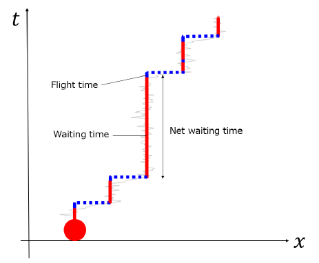
Figure 2: Schematic figure of a biased CTRW with flight times. The thin line is a trajectory of a Brownian motion under a tilted periodic potential. The solid line is a trajectory of a biased CTRW with flight times, where the net waiting time is a sum of waiting times and flight times.

III RESULT

III.1 Transition probabilities

Here, we analytically estimate the transition probabilities of a Brownian particle in a tilted periodic potential (see Fig. 1). Transition probabilities $p$ and $q$ are the probabilities of stepping from the bottom to the right and the left top, respectively. Transition probabilities $r$ and $s$ are the probabilities of stepping from the top to the right and the left bottom, respectively. The transition probabilities $p,q,r,{\color[rgb]{0,0,0}l}$ are obtained analytically for a general potential [30]. Using stable and unstable points of $U(x)$, we have the transition probabilities $p$ and $q$:

$$p=\frac{\int_{x_{2}}^{x_{3}}e^{\beta U(y)}dy}{\int_{x_{2}}^{x_{4}}e^{\beta U(y)}dy},q=\frac{\int_{x_{3}}^{x_{4}}e^{\beta U(y)}dy}{\int_{x_{2}}^{x_{4}}e^{\beta U(y)}dy},$$ (5)

where $\beta$ is the inverse temperature, i.e., $\beta=1/(k_{\rm B}T)$, $x_{2}$ and $x_{4}$ are unstable points, $x_{3}$ is a stable point of potential $U(x)$. Moreover, the transition probabilities $r$ and $l$ are also given by

$$r=\frac{\int_{x_{3}}^{x_{4}}e^{\beta U(y)}dy}{\int_{x_{3}}^{x_{5}}e^{\beta U(y)}dy},l=\frac{\int_{x_{4}}^{x_{5}}e^{\beta U(y)}dy}{\int_{x_{3}}^{x_{5}}e^{\beta U(y)}dy},$$ (6)

where $x_{5}$ is a stable point. Because $U(x)$ is a periodic tilted potential, probabilities $r$ and $l$ are also described by

$$r=\frac{\int_{x_{1}}^{x_{2}}e^{\beta U(y)}dy}{\int_{x_{1}}^{x_{3}}e^{\beta U(y)}dy}\ ,l=\frac{\int_{x_{2}}^{x_{3}}e^{\beta U(y)}dy}{\int_{x_{1}}^{x_{3}}e^{\beta U(y)}dy},$$ (7)

where $x_{1}$ is a stable point. From Eqs. (5) and (6), equalities $p+q=1$ and $r+l=1$ are satisfied.

III.2 Diffusion coefficient

In CTRWs, a stepping from the bottom to either the left or the right bottom occurs immediately as quickly as an assigned waiting time is over. However, in a Brownian motion in a tilted periodic potential, a step from a bottom to either the left or the right bottom may not be completed even if the particle reaches the left or the right top. It is important to note that in Brownian motion, the particle can return to the original bottom after it reaches the left or right top. Therefore, the probability density function (PDF) of net waiting time $T$ is not equal to that of waiting time $\tau$. Let $\phi(t)$, $\chi(t)$, and $\omega(t)$ be the PDFs of the time for a Brownian particle to move from the original bottom and return to the original bottom after reaching the left or the right top, the time for a Brownian particle to move from the original bottom to the right or the left bottom, and $\tau+\theta$, respectively. We note that the PDF of waiting time $\tau_{-}$ for a Brownian particle to move from a bottom to the left top of the potential before reaching the right top is the same as that $\tau_{+}$ for a Brownian particle to move from a bottom to the right top of the potential before reaching the left top. This equivalence is because both waiting times are defined by $\tau\equiv\min(\tau_{+},\tau_{-})$. By a simple calculation, the Laplace transforms of $\phi(t)$ and $\chi(t)$ with respect to $t$ become

$$\widetilde{\phi}(s) =(pl+qr)\ \widetilde{\omega}(s),$$ (8)

$$\widetilde{\chi}(s) =(pr+ql)\ \widetilde{\omega}(s).$$ (9)

We denote the Laplace transform of function $f(t)$ with respect to $t$ by $\widetilde{f}(s)$. Net waiting time $T$ is the time required for a Brownian particle to move from a bottom to one of the next neighboring bottoms. When a Brownian particle jumps to the next neighboring well after it moves a top and returns to the original well $n-1$ times, net waiting time $T$ is a $n$-times sum of $\tau+\theta$. Therefore, the PDF of net waiting time $T$, $\psi(t)$, is given by

$$\widetilde{\psi}(s)=\widetilde{\chi}(s)\sum_{n=1}^{\infty}\widetilde{\phi}^{n-1}(s)=\frac{\widetilde{\chi}(s)}{1-\widetilde{\phi}(s)},$$ (10)

where we used the fact that the distribution of the sum of random variables can be expressed by the product of the corresponding Laplace transformations. Furthermore, using a formula between the moments of a random variable and the Laplace transform of the PDF, i.e.,

$$\left.E[T^{r}]=(-1)^{r}\frac{d^{r}\widetilde{\psi}(s)}{ds^{r}}\right|_{s=0},$$ (11)

where $E[\cdot]$ represents the expectation value, we have the mean $\mu$ and the variance $\sigma^{2}$ of the net waiting time:

$$\mu =\frac{E[\tau]+E[\theta]}{pr+ql},$$ (12)

$$\sigma^{2} =\frac{V[\tau]+V[\theta]}{pr+ql}+\frac{pl+qr}{(pr+ql)^{2}}(E[\tau]+E[\theta])^{2},$$ (13)

where $V[\tau]$ and $V[\theta]$ are the variances of $\tau$ and $\theta$, respectively. Moreover, probability $P^{+}$ of moving from a bottom to the next right bottom is given by

$$P^{+}=pr\sum_{n=1}^{\infty}(pl+qr)^{n-1}=\frac{pr}{pr+ql}.$$ (14)

The probability $P^{+}$ can be also derived from the detailed balance equation. The detailed balance equation yields

$$\frac{\gamma(z\to z^{\prime})}{\gamma(z^{\prime}\to z)}=e^{\beta(U(z^{\prime})-U(z))},$$ (15)

where $\gamma(z\to z^{\prime})$ is the rate (probability per unit time) of transition from point $z$ to $z^{\prime}$. It follows that the ratio of rates $\gamma(x_{0}\to x_{0}+L)$ and $\gamma(x_{0}+L\to x_{0})$ becomes

$$\frac{\gamma(x_{0}\to x_{0}+L)}{\gamma(x_{0}+L\to x_{0})}=e^{\beta FL}~{}.$$ (16)

The rates $\gamma(x_{0}\to x_{0}+L)$ and $\gamma(x_{0}+L\to x_{0})$ can be represented by the mean net waiting time $\langle T\rangle$ and probabilities $P^{+}$ and $P^{-}$:

$$\gamma(x_{0}\to x_{0}+L)=\frac{P^{+}}{\langle T\rangle},$$

$$\gamma(x_{0}+L\to x_{0})=\frac{P^{-}}{\langle T\rangle}.$$ (17)

Therefore, we have $P^{-}=P^{+}e^{-\beta FL}$. Substituting this relation into $P^{+}+P^{-}=1$, the external force dependence of $P^{+}$ is given by

$$P^{+}=\frac{\exp(\beta FL/2)}{\exp(\beta FL/2)+\exp(-\beta FL/2)}.$$ (18)

We calculate the diffusion coefficient of a biased CTRW with flight times, where the lattice constant is $L$. We denote the number of jumps of a random walker from a bottom to the next neighboring bottom until time $t$ by $N_{t}$. Net waiting times $T$ are IID random variables. Therefore, $N_{t}$ is described by a renewal process [31]. By the renewal theory, the mean $\langle N_{t}\rangle$ and the variance $\langle\Delta N^{2}_{t}\rangle$ of $N_{t}$ are given by

$$\langle N_{t}\rangle =\frac{1}{\mu}t+O(1),$$ (19)

$$\langle\Delta N^{2}_{t}\rangle =\frac{\sigma^{2}}{\mu^{3}}t+O(1),$$ (20)

in the long-time limit. The results are valid when $\mu$ and $\sigma^{2}$ are finite. The variance of the displacement in a biased CTRW with flight times is given by

$$\langle\Delta x^{2}_{t}\rangle=4P^{+}P^{-}L^{2}\langle N_{t}\rangle+(P^{+}-P^{-})^{2}L^{2}\langle\Delta N_{t}^{2}\rangle.$$ (21)

We define the diffusion coefficient $D$ as

$$D:=\lim_{t\to\infty}\frac{\langle\Delta x^{2}_{t}\rangle}{2t}.$$ (22)

Substituting Eqs. (19), (20), (21) into Eq. (22) yields

$$D=\frac{L^{2}}{2}\quantity(\frac{4P^{+}(1-P^{+})}{\mu}+\frac{(2P^{+}-1)^{2}\sigma^{2}}{\mu^{3}}).$$ (23)

We note that transition probabilities $P_{\pm}$, $\mu$, and $\sigma^{2}$ are functions of external force $F$ in diffusion in a tilted potential.

III.3 Universality of giant diffusion

We investigate how the GD can be observed in the biased CTRW with flight times. In particular, we obtain the dependence of the diffusion coefficient (23) on external force $F$ and show that GD can be observed in general symmetric periodic potentials, especially for small temperatures. Let $\Delta E$ be the barrier energy of the tilted periodic potential $U(x)$, that is, the difference between the minimum and the right maximum of the potential. We denote barrier energy $\Delta E$ when $F=0$ by $\Delta E_{0}$.

First, we show that the diffusion coefficient is increased when the external force $F$ is small, i.e., $FL/2\ll\Delta E_{0}$. We also assume that the Arrhenius law is valid. In particular, we assume that the temperature is much smaller than the energy barrier, i.e. $\beta\Delta E\gg 1$ [32]. The Arrhenius law states that the exit times $\tau$ from a well with barrier energy $\Delta E$ follow an exponential distribution where the mean exit time is proportional to $\exp(\beta\Delta E)$. With the aid of the exponential distribution, the variance of $\tau$ is equal to the square of the mean, i.e., $V[\tau]=E[\tau]^{2}$. For $\beta\Delta E\gg 1$, $E[\tau]$ is much larger than $E[\theta]$. It follows that the variance of net waiting time is approximately equal to the square of the mean net waiting time, i.e., $\sigma^{2}\cong\mu^{2}$. Using Eq. (23) and $\sigma^{2}\cong\mu^{2}$, we have the diffusion coefficient $D_{\rm{small}}$ for small external force:

$$D_{\rm{small}}\simeq\frac{L^{2}}{2\mu}.$$ (24)

This relation can also be obtained directly from Eq. (23) by using $P_{+}\sim 1/2$ for $F\to 0$. Therefore, the dependence of $D_{\rm{small}}$ on external force $F$ is determined by $1/\mu$. The mean of the net waiting time $\mu$ depends on external force $F$, and the derivative is negative, i.e., $d\mu/dF<0$, because $\mu$ is proportional to $\exp(\beta\Delta E)$ and $\Delta E$ decreases as the external force is increased, i.e., $d\Delta E/dF<0$. Therefore, the derivative of $D_{\rm{small}}$ with respect to $F$ is positive:

$$\frac{dD_{\rm{small}}}{dF} =-\frac{L^{2}}{2\mu^{2}}\frac{d\mu}{dF}>0.$$ (25)

Thus, the diffusion coefficient $D$ increases as $F$ increases when the external force is small.

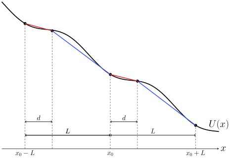
Figure 3: Coarse graining of a tilted periodic potential. The slope of the red straight line is $-a^{-}$, and the slope of the blue straight line is $-a^{+}$. Point $d$ is in between 0 and $L$.

Next, we show that the diffusion coefficient is decreased when the external force is large, i.e., $FL/2\gg\Delta E_{0}$. Because the contribution of the external force to the Brownian dynamics is much larger than that of the periodic potential, it can be regarded as Brownian motion under a constant external force. However, if we simply consider the Brownian motion under a constant external force, we obtain Einstein’s relation, i.e., $D=D_{E}$. Therefore, we consider a coarse-grained model of the tilted periodic potential by approximating the tilted potential as a piece-wise linear potential (see Fig.3). Point $d$ in Fig. 3 is an arbitrary coordinate and satisfies $0<d<L$. The slopes of the piece-wise linear potential are given by

$$a^{-} :=-\frac{V(x_{0}+d)-V(x_{0})-Fd}{d}~{}{\rm for}~{}0<\tilde{x}<d~{},$$ (26)

$$a^{+} :=-\frac{V(x_{0})-V(x_{0}+d)-F(L-d)}{L-d}~{}{\rm for}~{}d<\tilde{x}<L~{},$$ (27)

where $\tilde{x}=x-x_{0}-kL$ and $k$ is integer. In diffusion under a constant external force $F_{0}$, i.e., $F=F_{0}$ and $V(x)=0$ in Eq. (2), mean $\mu_{0}$ and variance $\sigma^{2}_{0}$ of the time for a Brownian particle to move a distance $y$ is given by [33]

$$\mu_{0}=\frac{\eta y}{F_{0}},~{}\sigma^{2}_{0}=\frac{2D_{\rm E}\eta^{3}y}{F_{0}^{3}}.$$ (28)

When the external force is large, there is no well in the tilted periodic potential. Moreover, $P_{+}\cong 1$ for large $F$. In the coarse-grained piece-wise linear potential, the mean and variance of the net waiting time $T$ become

$$\mu =\eta\quantity(\frac{d}{a^{-}}+\frac{L-d}{a^{+}}),$$ (29)

$$\sigma^{2} =2D_{E}\eta^{3}\quantity(\frac{d}{(a^{-})^{3}}+\frac{L-d}{(a^{+})^{3}}).$$ (30)

It follows that the diffusion coefficient $D_{\rm{large}}$ for large $F$ is given by

$$D_{\rm{large}}\simeq\frac{L^{2}}{2}\frac{\sigma^{2}}{\mu^{3}}=\frac{L^{2}}{\beta\eta}\frac{(a^{+})^{3}d+(a^{-})^{3}(L-d)}{\quantity(a^{+}d+(L-d)a^{-})^{3}}.$$ (31)

The derivative of $D_{\rm{large}}$ with respect to $F$ becomes negative:

$$\frac{dD_{\rm{large}}}{dF}=\frac{3\quantity(a^{-}-a^{+})^{2}(a^{-}+a^{+})d(d-L)}{(da^{+}+(L-d)a^{-})^{4}}\frac{4}{\beta\eta}<0,$$ (32)

where we used the fact that $da^{\pm}/dF=1$. When the external force is large, $D$ decreases as $F$ increases and converges to $D_{E}$ as $F\to\infty$. Therefore, we find that $D$ increases with small $F$ and decreases with large $F$. In other words, it is shown that there is at least one maximum at intermediate $F$ in the diffusion coefficient for general tilted periodic potentials. This peak is universal in the sense that it is observed for any tilted periodic potentials. Moreover, the diffusion coefficient at the peak is significantly enhanced especially for low temperature regimes. Therefore, giant diffusion is universally observed, especially for low-temperature regimes.

III.4 Giant diffusion in three tilted periodic potentials

We show giant diffusion for three symmetric periodic potentials as concrete examples. We note that $\Delta E_{0}$ is the barrier energy when there is no external force, and $L$ is the period. The first example is a sine potential (see Fig. 4a) :

$$V(x)=-\frac{\Delta E_{0}}{2}\cos{\quantity(\frac{2\pi}{L}x)}.$$ (33)

The second example is a sawtooth potential (see Fig. 4b):

$$V(x)=\frac{2\Delta E_{0}}{L}\absolutevalue{x-kL}~{}{\rm for}~{}\absolutevalue{x-kL}<L/2$$ (34)

where $k$ is integer. The sawtooth potential is a piecewise linear approximation of the sine potential. In numerical simulations, the force at $x=kL$ is set to be 0. The third example is an isosceles-trapezoid potential (see Fig. 4c):

$$V(x)=\begin{cases}0&{\rm for}~{}\absolutevalue{x-kL}<L/4-\varepsilon/2,\\ \\ \dfrac{\Delta E_{0}}{\varepsilon}(\absolutevalue{x-kL}-L/4)+\Delta E_{0}/2&{\rm for}~{}\absolutevalue{x-(k\pm 1/4)L}<\varepsilon/2,\\ \\ \Delta E_{0}&{\rm for}~{}\absolutevalue{x-kL}>L/4+\varepsilon/2,\end{cases}$$ (35)

where we assume $L>\varepsilon/2$. The isosceles trapezoid potential has straight lines with finite slopes $\pm\Delta E_{0}/\varepsilon$ in intervals with length $\varepsilon$ (see Fig. 4c). In the limit $\varepsilon\to 0$, it becomes a rectangular (square) potential. The isosceles-trapezoid potential is a generalization of the sawtooth potential. In particular, when $\varepsilon=L/2$, it becomes a sawtooth potential.

We apply our theory of the diffusion coefficient for a biased CTRW with flight times to the three periodic potentials by numerical simulations and compare the results with the result of Reimman et al., i.e., Eq. (3). Figure 5 shows the diffusion coefficients as a function of external force $F$ for the three periodic potentials. Giant diffusion is observed for the three periodic potentials. Our results of a biased CTRW with flight times are in good agreement with those of Reimman’s result. In numerical simulations of the Langevin equation (2), the simulation was performed by discretizing Eq. (2) using Euler’s method. In addition, white Gaussian noise $\xi(t)$ was generated using the Box-Muller method. To estimate $\mu$ and $\sigma^{2}$ in Eq.(23), we calculate the first passage time that a trajectory reaches the absorption boundary $x_{0}\pm L$, where $x_{0}$ is the starting point of the trajectory. For the sine potential, $x_{0}$ is defined by subcritical force $F_{s}=\pi\Delta E_{0}/L$:

$$x_{0}=\begin{cases}\dfrac{L}{2\pi}\arcsin\quantity(\dfrac{F}{F_{s}})&{\rm for}~{}0<F<F_{s}\\ \\ \dfrac{L}{4}&{\rm for}~{}F_{s}<F\end{cases}.$$ (36)

For sawtooth and isosceles-trapezoid potentials, $x_{0}$ is $x_{0}=0$.

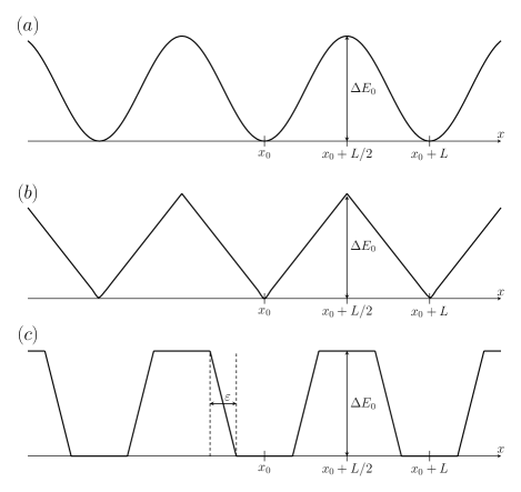
Figure 4: Three symmetric periodic potentials, where the difference between the minimum and maximum of the potential is set to be $\Delta E_{0}$. $(a)$ Sine potential. $(b)$ Sawtooth potential. $(c)$ Isosceles-trapezoid potential.

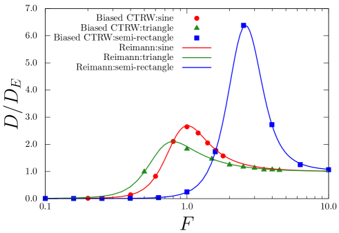
Figure 5: External force dependence of the diffusion coefficient for the three periodic potentials. We use $\beta=5,\eta=1,L=2\pi,\Delta E_{0}=2$ for all the potentials, and $\varepsilon=\pi/5$ in the isosceles trapezoidal potential. The solid line represents the results of Reimman et al., i.e., Eq. (3), by numerical integration. The symbols represent the results of a biased CTRW with flight times, i.e., Eq. (23), where parameters $\mu$ and $\sigma^{2}$ are estimated from simulation of the Langevin equation (2) and $P^{+}$ is calculated from (18).

III.5 Asymptotic behaviors of the diffusion coefficient

Here, we show the asymptotic behaviors of the diffusion coefficient in a tilted sawtooth potential for a large- and small-external force and large- and low-temperature limits. For the large-$F$ limit, we obtain the Einstein’s relation, i.e., $D=D_{E}$. This is valid for any periodic potentials.

In a tilted sawtooth potential, expanding Eq. (23) near $F=0$ yields

$$D=\frac{e^{\beta V}V^{2}\beta}{(1-e^{\beta V})\eta}+O(F^{2}).$$ (37)

For small-$F$ limit, the diffusion coefficient behaves as $D-D_{0}\propto F^{2}$, where $D_{0}$ is the diffusion coefficient for $F=0$. Because periodic potential $V(x)$ is symmetric, the order of the sub-leading term is $O(F^{2})$ in general. Furthermore, expanding Eq. (37) around $\beta=0$ gives

$$D=\frac{1}{\beta\eta}+O(\beta)+O(F^{2}).$$ (38)

Therefore, the diffusion coefficient converges to $D_{E}$, i.e., the Einstein relation holds, in the high-temperature limit even when the external force is small. This means that the situation is almost the same as that of free diffusion because large thermal noises overcome the potential. Furthermore, for a low-temperature limit $\beta\rightarrow\infty$ in Eq. (37), the diffusion coefficient becomes

$$D\simeq\frac{V^{2}\beta e^{-\beta V}}{\eta}\rightarrow 0.$$ (39)

This means that diffusion rarely occurs at a low-temperature limit.

Figure 6 shows critical force $F_{c}$ and the maximal diffusion coefficient $D_{c}$ in a tilted periodic sawtooth potential, where the critical force is defined by the force at which the diffusion coefficient is maximized. In numerical simulations, we use a biased CTRW with flight times, where parameters $\mu$ and $\sigma^{2}$ are calculated using Eqs. (12), (13), (18), (42), (43), (A), (47), (A), and (51) in Appendix A. We have confirmed that these analytical values are consistent with those in numerical simulations. Critical force $F_{c}$ converges to a constant value as $\beta$ increases. The value of $D_{c}/D_{0}$ significantly increases as $\beta$ increases.

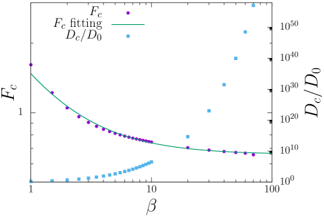
Figure 6: Critical force $F_{c}$ and the maximum value diffusion coefficient divided by $D_{0}$, i.e., $D_{c}/D_{0}$, as a function of inverse temperature $\beta$ in a biased CTRW with flight times, where parameters $\mu,\sigma^{2}$ and $P_{+}$ in Eq. (23) are obtained by Eqs. (12), (13), (18), (42), (43), (A), (47), (A), and (51) in the sawtooth potential with $L=2\pi$ and $\Delta E_{0}=2$. Circles and squares are the results on numerical simulations for $F_{c}$ and $D_{c}/D_{0}$, respectively. The solid curve is a fitting of critical force $F_{c}$ by $F_{c}=A/\beta+B$ with $A=0.817697$ and $B=0.657699$.

IV Conclusion

We construct a coarse-grained stochastic model of a Brownian motion in a tilted symmetric periodic potential by a biased CTRW with flight times. We derive the diffusion coefficient of the biased CTRW model with flight times by the renewal theory. Compared to the Reimann’s result, i.e., Eq. (3), our expression of the diffusion coefficient is much more simple. Thus, we obtain an explicit dependence of the diffusion coefficient on the external force for small and large forces. As a result, we show the universality of giant diffusion in tilted symmetric periodic potentials in the sense that there is at least one peak in the diffusion coefficient and the peak value is significantly larger than that without external force. We apply our theory to three periodic tilted potentials. We can derive the diffusion coefficients as a function of $F$ if we evaluate $\mu$ and $\sigma^{2}$. Our theory can also be applied to non-symmetric periodic potentials. It is not straightforward to show the universality of the giant diffusion because the diffusion coefficient for small external force $F$ may decreases as $F$ increases. However, we think that giant diffusion will be universally observed in tilted non-symmetric periodic potentials. Moreover, even in higher dimensional systems, giant diffusion can be observed when diffusion directed to the applied force is independent of other directions. By numerical simulations, we confirm the validity of our theory and the giant diffusion for three tilted periodic potentials.

Appendix A External force dependence of physical quantities in sawtooth potential

Here, we provide external force dependence of some statistical quantities in a tilted periodic sawtooth potential. In what follows, we use the following notation:

$$b^{\pm}:=2V_{0}\pm FL~{}.$$ (40)

Therefore, the tilted sawtooth potential $U_{{\rm saw}}(x)$ can be represented as

$$U_{{\rm saw}}(x)=\begin{cases}-\frac{b^{+}}{L}x+2\Delta E_{0}k&{\rm for}~{}(k-1)L/2\leq x<kL\\ +\frac{b^{-}}{L}x-2\Delta E_{0}k&{\rm for}~{}kL\leq x<(k+1)L/2\\ \end{cases},$$ (41)

where $k$ is integer. According to the formulas (5), (6), we obtain the external force dependence of the probabilities $p,r,P^{+}$:

$$p =\frac{\frac{1}{b^{+}}(e^{\beta\frac{b^{+}}{2}}-1)}{\frac{1}{b^{+}}(e^{\beta\frac{b^{+}}{2}}-1)+\frac{1}{b_{-}}(e^{\beta\frac{b^{-}}{2}}-1)},$$ (42)

$$r =\frac{\frac{1}{b^{-}}(e^{\beta\frac{b^{-}}{2}}-1)}{\frac{1}{b^{-}}(e^{\beta\frac{b^{-}}{2}}-1)+\frac{1}{b_{+}}(1-e^{-\beta\frac{b^{+}}{2}})e^{\beta\frac{b^{-}}{2}}}~{},$$ (43)

$$P^{+} =\frac{\exp(\beta FL/2)}{\exp(\beta FL/2)+\exp(-\beta FL/2)}.$$ (44)

These results agree with numerical results (see Fig. 7).

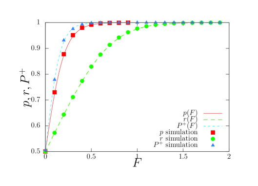
Figure 7: External Force dependence of probabilities $p,r,P^{+}$. Symbols are the results of numerical simulations, where we set $\beta=2$. The red solid, the green dashed, and the blue dotted lines represent $p(F)$, $r(F)$, and $P^{+}$, respectively.

The $n$th moment of FPT, which is the time for a Brownian particle to move from the initial position $x=x_{0}$ to the absorbing boundary $x=A$ or $x=B$ (where $A\leq x\leq B$), is given by the following formula [30]:

$$T_{n}(x)=\beta\eta n\quantity(\frac{(\int_{A}^{x}e^{\beta U(y)}dy)\int_{x}^{B}e^{\beta U(y)}dy\int_{A}^{y}e^{-\beta U(z)}T_{n-1}(z)dz}{\int_{A}^{B}e^{\beta U(y)}dy}-\frac{(\int_{x}^{B}e^{\beta U(y)}dy)\int_{A}^{x}e^{\beta U(y)}dy\int_{A}^{y}e^{-\beta U(z)}T_{n-1}(z)dz}{\int_{A}^{B}e^{\beta U(y)}dy}).$$ (45)

Therefore, the 1st moment of $\tau$ is represented by

$$E[\tau]= \frac{L^{2}\eta}{\beta}\frac{b^{+}b^{-}}{b^{-}\quantity(e^{\beta\frac{b^{+}}{2}}-1)+b^{+}\quantity(e^{\beta\frac{b^{-}}{2}}-1)}$$

$$\times \left\{\frac{1}{(b^{+})^{2}b^{-}}\quantity(e^{\beta\frac{b^{-}}{2}}-1)\quantity(e^{\beta\frac{b^{+}}{2}}-1-\beta\frac{b^{+}}{2})\right.\left.+\frac{1}{b^{+}(b^{-})^{2}}\quantity(e^{\beta\frac{b^{+}}{2}}-1)\quantity(e^{\beta\frac{b^{-}}{2}}-1-\beta\frac{b^{-}}{2})\right\},$$ (46)

and the 2nd moment of $\tau$ is given by

$$E[\tau^{2}]=2(pI_{p}-qI_{m}),$$ (47)

where

$$I_{p}= \frac{L^{4}\eta^{2}}{\beta^{4}}\frac{b^{+}b^{-}}{b^{-}\quantity(e^{\frac{\beta b^{+}}{2}}-1)+b^{+}\quantity(e^{\frac{\beta b^{-}}{2}}-1)}$$

$$\times \left\{\frac{1}{(b^{-})^{5}}\quantity[\quantity(e^{\frac{\beta b^{-}}{2}}-1+\frac{\beta b^{-}}{2})\quantity(e^{\frac{\beta b^{-}}{2}}-1-\frac{\beta b^{-}}{2})+\frac{\beta b^{-}}{2}\quantity(e^{\frac{\beta b^{-}}{2}}-1)+\frac{(\beta b^{-})^{2}}{8}\quantity(1-3e^{\frac{\beta b^{-}}{2}})]\right.$$

$$\left.+\frac{1}{(b^{-})^{4}b^{+}}\quantity(e^{\frac{\beta b^{+}}{2}}-1)\quantity[\quantity(e^{\frac{\beta b^{-}}{2}}+1-\frac{\beta b^{-}}{2})\quantity(e^{\frac{\beta b^{-}}{2}}-1-\frac{\beta b^{-}}{2})-\quantity(1-e^{\frac{\beta b^{-}}{2}})-\frac{\beta b^{-}}{2}e^{\frac{\beta b^{-}}{2}}-\frac{(\beta b^{-})^{2}}{8}]\right.$$

$$\left.+\frac{1}{(b^{-})^{3}(b^{+})^{2}}\quantity(e^{\frac{\beta b^{+}}{2}}-1-\frac{\beta b^{+}}{2})\quantity(2e^{\beta b^{-}}-2e^{\beta\frac{b^{-}}{2}}-\frac{3}{2}\beta b^{-}e^{\frac{\beta b^{-}}{2}}+\frac{\beta b^{-}}{2})\right.$$

$$\left.+\frac{1}{(b^{-})^{2}(b^{+})^{3}}\quantity(e^{\frac{\beta b^{+}}{2}}-e^{-\frac{\beta b^{+}}{2}}-\beta b^{+})\quantity(e^{\frac{\beta b^{-}}{2}}-1)^{2}\right.$$

$$\left.+\frac{1}{b^{-}(b^{+})^{4}}\quantity(e^{\frac{\beta b^{+}}{2}}-e^{-\frac{\beta b^{+}}{2}}-2-\frac{(\beta b^{+})^{2}}{4})\quantity(e^{\frac{\beta b^{-}}{2}}-1)\right\}$$ (48)

and

$$I_{m}= \frac{L^{4}\eta}{\beta^{3}}\frac{b^{+}b^{-}}{b^{-}\quantity(e^{\frac{\beta b^{+}}{2}}-1)+b^{+}\quantity(e^{\frac{\beta b^{-}}{2}}-1)}$$

$$\times \left\{\frac{1}{(b^{+})^{5}}\quantity[\quantity(2-e^{\frac{\beta b^{+}}{2}}-e^{-\frac{\beta b^{+}}{2}})+\frac{\beta b^{+}}{2}\quantity(1-e^{\frac{\beta b^{+}}{2}})+\frac{(\beta b^{+})^{2}}{8}(3+e^{\frac{\beta b^{+}}{2}})]\right.$$

$$\left.+\frac{1}{(b^{+})^{4}b^{-}}\quantity(e^{\frac{\beta b^{-}}{2}}-1)\quantity[\quantity(1+e^{-\frac{\beta b^{+}}{2}}-2e^{\frac{\beta b^{+}}{2}})+\beta b^{+}\quantity(1+\frac{1}{2}e^{\frac{\beta b^{+}}{2}})-\frac{(\beta b^{+})^{2}}{8}]\right.$$

$$\left.+\frac{1}{(b^{+})^{3}(b^{-})^{2}}\quantity(e^{\frac{\beta b^{-}}{2}}-1-\frac{\beta b^{-}}{2})\quantity[2\quantity(1-e^{\frac{\beta b^{+}}{2}})+\frac{\beta b^{+}}{2}\quantity(1+e^{\frac{\beta b^{+}}{2}})]\right\}.$$ (49)

In the same way of the calculation of $\tau$, the 1st moment of $\theta$ is given by

$$E[\theta]= \frac{L^{2}\eta}{\beta}\frac{b^{+}b^{-}}{b^{+}\quantity(e^{\beta\frac{b^{-}}{2}}-1)+b^{-}e^{2\beta V_{0}}\quantity(e^{-\beta\frac{b^{+}}{2}}-e^{-\beta b^{+}})}$$

$$\times \left\{\frac{1}{b^{+}(b^{-})^{2}}e^{2\beta V_{0}}\quantity(e^{-\beta\frac{b^{+}}{2}}-e^{-\beta b^{+}})\quantity(e^{-\beta\frac{b^{-}}{2}}-1-\beta\frac{b^{-}}{2})\right.\left.+\frac{1}{(b^{+})^{2}b^{-}}\quantity(e^{\beta\frac{b^{-}}{2}}-1)\quantity(e^{-\beta\frac{b^{+}}{2}}-1+\beta\frac{b^{+}}{2})\right\},$$ (50)

and the 2nd moment of $\theta$ is given by

$$E[\theta^{2}]=2(rJ_{p}-sJ_{m}),$$ (51)

where,

$$J_{p}= \frac{L^{4}\eta^{2}}{\beta^{2}}\frac{b^{+}b^{-}}{b^{+}\quantity(e^{\beta\frac{b^{-}}{2}}-1)+b^{-}e^{2\beta V_{0}}\quantity(e^{-\beta\frac{b^{+}}{2}}-e^{-\beta b^{+}})}$$

$$\times \left\{\frac{e^{2\beta V_{0}}}{(b^{+})^{5}}\quantity[-\quantity(e^{\frac{3\beta b^{+}}{2}}-2e^{-\beta b^{+}}+\frac{\beta b^{+}}{2})+\frac{\beta b^{+}}{2}\quantity(e^{-\beta b^{+}}-e^{\frac{-\beta b^{+}}{2}})+\frac{(\beta b^{+})^{2}}{8}\quantity(3e^{-\beta b^{+}}-e^{-\frac{\beta b^{+}}{2}})]\right.$$

$$\left.+\frac{1}{(b^{+})^{4}b^{-}}\quantity(e^{\frac{\beta b^{-}}{2}}-1)\quantity[\quantity(e^{-\beta b^{+}}+e^{-\frac{\beta b^{+}}{2}}-2)+\frac{3\beta b^{+}}{2}e^{-\frac{\beta b^{+}}{2}}+\frac{(\beta b^{+})^{2}}{8}]\right.$$

$$\left.+\frac{e^{2\beta V_{0}}}{(b^{+})^{3}(b^{-})^{2}}\quantity(e^{-\frac{\beta b^{-}}{2}}-1+\frac{\beta b^{-}}{2})\quantity[2\quantity(e^{-\beta b^{+}}-e^{-\beta\frac{3b^{+}}{2}})+\frac{\beta b^{+}}{2}\quantity(e^{-\frac{\beta b^{+}}{2}}-3e^{-\beta b^{+}})]\right.$$

$$\left.+\frac{e^{4\beta V_{0}}}{(b^{+})^{2}(b^{-})^{3}}\quantity(1-e^{-\beta b^{-}}-\beta b^{-}e^{-\beta\frac{b^{-}}{2}})\quantity(e^{-\frac{\beta b^{+}}{2}}-e^{-\beta b^{+}})^{2}\right.$$

$$\left.+\frac{1}{b^{+}(b^{-})^{4}}\quantity(e^{\frac{\beta b^{-}}{2}}+e^{-\frac{\beta b^{-}}{2}}-2-\frac{(\beta b^{-})^{2}}{4})\quantity(e^{-\frac{\beta b^{+}}{2}}-e^{-\beta b^{+}})\right\},$$ (52)

$$J_{m}= \frac{L^{4}\eta^{2}}{\beta^{2}}\frac{b^{+}b^{-}}{b^{+}\quantity(e^{\beta\frac{b^{-}}{2}}-1)+b^{-}e^{2\beta V_{0}}\quantity(e^{-\beta\frac{b^{+}}{2}}-e^{-\beta b^{+}})}$$

$$\times \left\{\frac{1}{(b^{-})^{5}}\quantity[\quantity(e^{\beta b^{-}}-2e^{\beta\frac{b^{-}}{2}}+1)+\frac{\beta b^{-}}{2}\quantity(e^{\frac{\beta b^{-}}{2}}-1)+\frac{(\beta b^{-})^{2}}{8}(1+3e^{\frac{\beta b^{-}}{2}})]\right.$$

$$\left.+\frac{e^{2\beta V_{0}}}{(b^{-})^{4}b^{+}}\quantity(e^{-\frac{\beta b^{+}}{2}}-e^{-\beta b^{+}})\quantity[\quantity(e^{\frac{\beta b^{-}}{2}}-2e^{-\frac{\beta b^{-}}{2}}+1)-\frac{\beta b^{-}}{2}\quantity(2+e^{-\frac{\beta b^{-}}{2}})-\frac{(\beta b^{-})^{2}}{8}]\right.$$

$$\left.+\frac{1}{(b^{-})^{3}(b^{+})^{2}}\quantity(e^{-\frac{\beta b^{+}}{2}}-1+\frac{\beta b^{+}}{2})\quantity[2-2e^{\frac{\beta b^{-}}{2}}+\frac{\beta b^{-}}{2}\quantity(1+e^{\frac{\beta b^{-}}{2}})]\right\}.$$ (53)

Appendix B Generalized Montroll-Weiss formula for asymmetric waiting time time distributions

We consider a one-dimensional CTRW, in which the random walker takes steps with length distributions $\phi_{+}(\xi)$ and $\phi_{-}(\xi)$ to the right or to the left. After each step, two random waiting times $\tau_{+}$ and $\tau_{-}$ are independently drawn from two waiting time distributions $\psi_{+}(\tau)$ and $\psi_{-}(\tau)$, respectively. Then, the next step is taken to the right if $\tau_{+}\leq\tau_{-}$ and to the left otherwise. We want to compute the distribution of the random walker’s position $x=\sum_{j=1}^{N_{+}}\xi_{j,+}-\sum_{j=1}^{N_{-}}\xi_{j,-}$ at time $t$, where $N_{+}$ and $N_{-}$ are the number of steps taken to the right and left, respectively, and $\xi_{j,+}$ and $\xi_{j,-}$ are the corresponding step lengths. This can generally be written as

$$P(x,t)dx=\sum_{N_{+}=0}^{\infty}\sum_{N_{-}=0}^{\infty}\underbrace{\text{Pr}\bigg{(}x\leq\sum_{j=1}^{N_{+}}\xi_{j,+}-\sum_{j=1}^{N_{-}}\xi_{j,-}\leq x+dx\bigg{)}}_{\text{Prob. of steps summing to $x$}}\underbrace{\text{Pr}(N_{+},N_{-},t)\vphantom{\sum_{j=1}^{N_{-}}}}_{\text{Prob. of observing $N_{+}$/$N_{-}$ steps to the right/left up to time $t$}}.$$ (54)

Upon a spatial Fourier transform, the first term can be written as a product using the convolution theorem,

$$\hat{P}(k,t)=\sum_{N_{+}=0}^{\infty}\sum_{N_{-}=0}^{\infty}\hat{\phi}_{+}(k)^{N_{+}}\hat{\phi}^{*}_{-}(k)^{N_{-}}P(N_{+},N_{-},t),$$ (55)

where we denote the Fourier transform of a function by

$$\hat{f}(k)=\int_{-\infty}^{\infty}dx\ e^{ikx}f(x)$$ (56)

and $f^{*}(k)$ denotes complex conjugation. The joint probability of observing $N_{+}$ and $N_{-}$, steps to the right and left, can also be written as,

$$P(N_{+},N_{-},t)=P_{-}(N_{-}|N)P_{\pm}(N,t),$$ (57)

i.e., the probability of taking $N=N_{+}+N_{-}$ steps in total times the probability that $N_{-}$ out of those are to the left. The latter probability can be computed from the waiting time distributions as follows. Let us consider the probability of $\tau_{-}$ being smaller than $\tau_{+}$ for any one pair of waiting times,

$$p_{<}\equiv\text{Pr}(\tau_{-}<\tau_{+})=\int_{0}^{\infty}d\tau\ \psi_{-}(\tau)\int_{\tau}^{\infty}d\tau^{\prime}\ \psi_{+}(\tau^{\prime}).$$ (58)

Then, since the steps are independent, the probability of $N_{-}$ out of $N$ steps satisfying this condition is just the binomial distribution,

$$P_{-}(N_{-}|N)=\left(\begin{array}[]{c}N\\ N_{-}\end{array}\right)p_{<}^{N_{-}}(1-p_{<})^{N-N_{-}},$$ (61)

for $N_{-}\leq N$ and $0$ otherwise. This results in

$$\hat{P}(k,t)=\sum_{N=0}^{\infty}\sum_{N_{-}=0}^{N}\hat{\phi}_{+}(k)^{N-N_{-}}\hat{\phi}^{*}_{-}(k)^{N_{-}}\left(\begin{array}[]{c}N\\ N_{-}\end{array}\right)p_{<}^{N_{-}}(1-p_{<})^{N-N_{-}}P_{\pm}(N,t).$$ (64)

The sum over $N_{-}$ can now be evaluated,

$$\hat{P}(k,t)=\sum_{N=0}^{\infty}\hat{\phi}_{+}(k)^{N}\bigg{(}1+p_{<}\bigg{(}\frac{\hat{\phi}^{*}_{-}(k)}{\hat{\phi}_{+}(k)}-1\bigg{)}\bigg{)}^{N}P_{\pm}(N,t).$$ (65)

In order to compute $P_{\pm}(N,t)$, we note that the total waiting time can be written as

$$\tau_{\text{tot}}=\sum_{j=1}^{N}\text{min}\big{(}\tau_{j,+},\tau_{j,-}\big{)},$$ (66)

since at each step, the smaller of the two waiting times is chosen. Introducing the random variable $\tau=\text{min}(\tau_{+},\tau_{-})$, we can write its cumulative distribution function as

$$F(\tau)=\text{Pr}\big{(}\text{min}(\tau_{+},\tau_{-})\geq\tau\big{)}=\text{Pr}\big{(}\tau_{+}\geq\tau,\tau_{-}\geq\tau\big{)}=\text{Pr}(\tau_{+}\geq\tau)\text{Pr}(\tau_{-}\geq\tau),$$ (67)

since the waiting times for right and left steps are assumed to be independent. Taking the derivative with respect to $\tau$, we obtain for the waiting time distribution of steps in an arbitrary direction,

$$\psi(\tau)=-\partial_{\tau}F(\tau)=\psi_{+}(\tau)\int_{\tau}^{\infty}d\tau^{\prime}\ \psi_{-}(\tau^{\prime})+\psi_{-}(\tau)\int_{\tau}^{\infty}d\tau^{\prime}\ \psi_{+}(\tau^{\prime}).$$ (68)

Intuitively, this relation means that for the overall waiting time to be $\tau$, either we have $\tau_{+}=\tau$ and $\tau_{-}>\tau$ or vice versa (note that the border case $\tau_{+}=\tau_{-}$ is a zero-set and can be neglected, since the waiting times are distributed continuously). To obtain $P_{\pm}(N,t)$ from $\psi$, we note that it can be written as

$$P_{\pm}(N,t)=\int_{0}^{t}dt^{\prime}\ \psi_{N}(t^{\prime})\bar{P}(t-t^{\prime})=\int_{0}^{t}dt^{\prime}\ \psi_{N}(t^{\prime})\int_{t-t^{\prime}}^{\infty}dt^{\prime\prime}\ \psi(t^{\prime\prime}),$$ (69)

where $\psi_{N}(t^{\prime})$ is the PDF of the $N$-th step occurring at $t^{\prime}$ and $\bar{P}(t-t^{\prime})$ is the probability of no steps occurring in an interval of length $t-t^{\prime}$, i.e., the $N+1$-th waiting time being larger than $t-t^{\prime}$. As for the total displacement, $\psi_{N}(t)$ is given in terms of the sum over $N$ waiting times,

$$\psi_{N}(t)dt=\text{Pr}\bigg{(}t\leq\sum_{j=1}^{N}\tau_{j}\leq t+dt\bigg{)},$$ (70)

and its Laplace transform, by virtue of the convolution theorem, is given by

$$\tilde{\psi}^{*}_{N}(s)=\tilde{\psi}(s)^{N}.$$ (71)

Thus, we obtain for the Laplace transform of $P_{\pm}(N,t)$:

$$\tilde{P}_{\pm}(N,s)=\tilde{\psi}(s)^{N}\frac{1-\tilde{\psi}(s)}{s}.$$ (72)

Taking the Laplace transform of Eq. (65), we then get

$$\hat{\tilde{P}}(k,s)=\sum_{N=0}^{\infty}\hat{\phi}_{+}(k)^{N}\bigg{(}1+p_{<}\bigg{(}\frac{\hat{\phi}^{*}_{-}(k)}{\hat{\phi}_{+}(k)}-1\bigg{)}\bigg{)}^{N}\tilde{\psi}(s)^{N}\frac{1-\tilde{\psi}^{*}(s)}{s}.$$ (73)

Evaluating the sum over $N$ using the geometric series formula, we obtain

$$\hat{\tilde{P}}(k,s) =\frac{1-\tilde{\psi}^{*}(s)}{s\Big{(}1-\tilde{\psi}(s)\Big{(}\hat{\phi}_{+}(k)+p_{<}\big{(}\hat{\phi}^{*}_{-}(k)-\hat{\phi}_{+}(k)\big{)}\Big{)}\Big{)}}$$ (74)

$$\text{with}\qquad p_{<} =\int_{0}^{\infty}d\tau\ \psi_{-}(\tau)\int_{\tau}^{\infty}d\tau^{\prime}\ \psi_{+}(\tau^{\prime}),$$

where $\tilde{\psi}(s)$ is given by the convolution integral

$$\tilde{\psi}(s)=\tilde{\psi}_{+}(s)+\tilde{\psi}_{-}(s)-\frac{s}{2\pi i}\int_{\delta-i\infty}^{\delta+i\infty}d\sigma\ \frac{1}{\sigma(s-\sigma)}\tilde{\psi}_{+}(\sigma)\tilde{\psi}_{-}(s-\sigma).$$ (75)

Equation (74) is a generalization of the Montroll-Weiss formula to asymmetric waiting time and jump distributions. It expresses the Fourier-Laplace transform of the probability distribution in terms of the step size and waiting time distributions. We note that, similar to the original Montroll-Weiss formula, the symmetric waiting time distribution $\psi(\tau)$ determines the dynamics, the waiting time distributions for the right/left steps enter only via the asymmetry parameter $p_{<}$. We remark that for the special case $\bar{\psi}=\psi_{+}=\psi_{-}$, this $\bar{\psi}$ does not correspond to the waiting time distribution $\psi$ in the original Montroll-Weiss formula, since we take the minimum of the two times.

References

• [1] Robert Brown. Xxvii. a brief account of microscopical observations made in the months of june, july and august 1827, on the particles contained in the pollen of plants; and on the general existence of active molecules in organic and inorganic bodies. The philosophical magazine, 4(21):161–173, 1828.
• [2] Albert Einstein. Über die von der molekularkinetischen theorie der wärme geforderte bewegung von in ruhenden flüssigkeiten suspendierten teilchen. Annalen der physik, 4, 1905.
• [3] Paul Langevin. Sur la théorie du mouvement brownien. Compt. Rendus, 146:530–533, 1908.
• [4] Adolph Fick. V. on liquid diffusion. The London, Edinburgh, and Dublin Philosophical Magazine and Journal of Science, 10(63):30–39, 1855.
• [5] Hannes Risken and Hannes Risken. Fokker-planck equation. Springer, 1996.
• [6] Subrahmanyan Chandrasekhar. Stochastic problems in physics and astronomy. Reviews of modern physics, 15(1):1, 1943.
• [7] Elliott W Montroll and George H Weiss. Random walks on lattices. ii. Journal of Mathematical Physics, 6(2):167–181, 1965.
• [8] Ralf Metzler and Joseph Klafter. The random walk’s guide to anomalous diffusion: a fractional dynamics approach. Physics reports, 339(1):1–77, 2000.
• [9] Jean-Philippe Bouchaud and Antoine Georges. Anomalous diffusion in disordered media: statistical mechanisms, models and physical applications. Physics reports, 195(4-5):127–293, 1990.
• [10] François Bardou, J.-P. Bouchaud, A. Aspect, and C. Cohen-Tannoudji. Levy statistics and laser cooling: how rare events bring atoms to rest. Cambridge University Press, 2002.
• [11] Andreas Dechant, Farina Kindermann, Artur Widera, and Eric Lutz. Continuous-time random walk for a particle in a periodic potential. Physical review letters, 123(7):070602, 2019.
• [12] Y. He, S. Burov, R. Metzler, and E. Barkai. Random time-scale invariant diffusion and transport coefficients. Phys. Rev. Lett., 101:058101, 2008.
• [13] Tomoshige Miyaguchi and Takuma Akimoto. Intrinsic randomness of transport coefficient in subdiffusion with static disorder. Phys. Rev. E, 83:031926, 2011.
• [14] Tomoshige Miyaguchi and Takuma Akimoto. Ergodic properties of continuous-time random walks: Finite-size effects and ensemble dependences. Phys. Rev. E, 87:032130, Mar 2013.
• [15] Ralf Metzler, Jae-Hyung Jeon, Andrey G Cherstvy, and Eli Barkai. Anomalous diffusion models and their properties: non-stationarity, non-ergodicity, and ageing at the centenary of single particle tracking. Phys. Chem. Chem. Phys., 16(44):24128–24164, 2014.
• [16] Takuma Akimoto, Eli Barkai, and Keiji Saito. Universal fluctuations of single-particle diffusivity in a quenched environment. Phys. Rev. Lett., 117:180602, Oct 2016.
• [17] Takuma Akimoto, Eli Barkai, and Keiji Saito. Non-self-averaging behaviors and ergodicity in quenched trap models with finite system sizes. Phys. Rev. E, 97:052143, May 2018.
• [18] Ryunosuke Hayashi, Kazuo Sasaki, Shuichi Nakamura, Seishi Kudo, Yuichi Inoue, Hiroyuki Noji, and Kumiko Hayashi. Giant acceleration of diffusion observed in a single-molecule experiment on f 1- atpase. Physical review letters, 114(24):248101, 2015.
• [19] W Dieterich, P__ Fulde, and I Peschel. Theoretical models for superionic conductors. Advances in Physics, 29(3):527–605, 1980.
• [20] YMI Anchenko and LA Zil’Berman. The josephson effect in small tunnel contacts. Soviet Phys. JETP, 28, 1969.
• [21] Meng Su and Benjamin Lindner. Active brownian particles in a biased periodic potential. The European Physical Journal E, 46(4):22, 2023.
• [22] Yu Lu and Guo-Hui Hu. Giant acceleration of diffusion in soft matter potential. arXiv preprint arXiv:2310.08003, 2023.
• [23] Peter Reimann, Christian Van den Broeck, H Linke, Peter Hänggi, JM Rubi, and Agustın Pérez-Madrid. Giant acceleration of free diffusion by use of tilted periodic potentials. Physical review letters, 87(1):010602, 2001.
• [24] Peter Reimann, Christian Van den Broeck, H Linke, Peter Hänggi, JM Rubi, and Agustín Pérez-Madrid. Diffusion in tilted periodic potentials: Enhancement, universality, and scaling. Physical Review E, 65(3):031104, 2002.
• [25] William Feller. An Introduction to Probability Theory and Its Applications, volume 1. Wiley, New York, 1968.
• [26] R. Burioni, G. Gradenigo, A. Sarracino, A. Vezzani, and A. Vulpiani. Commun. Theor. Phys., 62:514, 2014.
• [27] Giacomo Gradenigo, Eric Bertin, and Giulio Biroli. Field-induced superdiffusion and dynamical heterogeneity. Phys. Rev. E, 93:060105(R), Jun 2016.
• [28] Takuma Akimoto, Andrey G. Cherstvy, and Ralf Metzler. Ergodicity, rejuvenation, enhancement, and slow relaxation of diffusion in biased continuous-time random walks. Phys. Rev. E, 98:022105, Aug 2018.
• [29] Ru Hou, Andrey G Cherstvy, Ralf Metzler, and Takuma Akimoto. Biased continuous-time random walks for ordinary and equilibrium cases: facilitation of diffusion, ergodicity breaking and ageing. Phys. Chem. Chem. Phys., 20(32):20827–20848, 2018.
• [30] Crispin Gardiner. Stochastic methods, volume 4. Springer Berlin, 2009.
• [31] DR Cox. Renewal theory (methuen, 1962). Cited on, page 418, 1967.
• [32] Peter Hänggi, Peter Talkner, and Michal Borkovec. Reaction-rate theory: fifty years after kramers. Reviews of modern physics, 62(2):251, 1990.
• [33] Annalisa Molini, Peter Talkner, Gabriel G Katul, and Amilcare Porporato. First passage time statistics of brownian motion with purely time dependent drift and diffusion. Physica A: Statistical Mechanics and its Applications, 390(11):1841–1852, 2011.