Nonclassicality in Two-Mode Stabilized Squeezed Coherent State: Quantum-to-Classical transition
Abstract
We consider a two-mode stabilized squeezed coherent state (SSCS) of light and introduce the indicator, a novel measure for characterizing nonclassicality in the resulting EPR-entangled state. Unlike existing methods based on Cauchy-Schwarz or Murihead inequalities, leverages analytical solutions to the quantum Langevin equations to directly analyze nonclassicality arising from key processes like bichromatic injection, frequency conversion, and parametric down-conversion (both spontaneous and stimulated). This approach not only identifies the optimal phase for maximum nonclassicality but also reveals two new phenomena: first, both intra-cavity and extra-cavity fields exhibit the same degree of nonclassicality, and second, balanced seeding in phase-mismatched configurations induces nonclassicality across a broad range of squeezing and seeding parameters. Our work deepens the understanding of the intricate dependence of nonclassicality on system parameters in the context of SSCS, paving the way for investigations into the quantum-to-classical transition in entangled systems. The potential of holds significant promise for advancements in quantum optics and information science.
I Introduction
Quantitative nonclassicality measures, crucial to quantum information science, enable the implementation of quantum information protocols [1, 2, 3, 4, 5] using controllable system parameters of quantum states. These protocols facilitate high-precision measurements [6, 7, 8, 9], surpassing the classical limitations imposed by quantum projection noise. Ultimately, these measures can help reveal the mechanisms behind the quantum-to-classical transition [10, 11, 12].
In quantum optics, for single-mode light, nonclassicality measures have been investigated based on various concepts, including quantum Fisher information [13, 14, 5], entanglement potential [15], nonclassical distance [16], Bures distance [17], nonclassical depth [18], and nonclassicality with positive semidefinite observables [19]. In the case of multi-mode light, different approaches are used. For example, nonclassicality measures are often parameterized by quantum contextuality [20, 21], logarithmic negativity of the covariance matrix [22], negative quasiprobability [23, 24, 25, 26], or violations of inequalities like the Cauchy-Schwarz and Murihead inequalities [27, 28, 29, 30, 31, 32, 33].
In particular, for two-mode entangled light, violation of classical inequalities, like the Cauchy-Schwarz inequality (CSI) [27], indicates the presence of strong quantum correlations between the modes (EPR-entanglement). For example, a state with a negative Glauber function [34, 35, 36] signifies a violation of the CSI [27]. Introduced by Agarwal [28], this criterion ( in Eq. (12)) characterizes the quantum properties of general two-mode states and remains applicable even in the single-photon regime. It incorporates both the mean values of self and cross-correlation functions for the two-mode number operators. Similarly, Lee proposed a slightly different definition for the second-order moment (SOM) criterion ( in Eq. (13)) based on the Murihead inequality, which is equivalent to the elementary arithmetic-geometric mean inequality and relies on the majorization of higher-order moments of number operators [29].
However, all-known nonclassicality measures fail to analytically quantify the contributions from individual quantum mechanisms within the quantum light source. This significantly hinders our ability to quantitatively reveal the quantum-to-classical transition as this system interacts with the environment.
This paper investigates the applicability of existing nonclassicality measures ( and ) to a two-mode stabilized squeezed coherent state (SSCS) generated by a seeded optical parametric oscillator (OPO) in the single-photon regime (Fig. 1). While and show the same expressions both inside and outside the OPO cavity, they fail to distinguish the separate contributions of individual system parameters. Our goal is to quantitatively understand how the quantum-to-classical transition of the SSCS depends on the strength of controllable system parameters.
To overcome limitations in existing nonclassicality measures’ ability to quantify individual quantum processes, we introduce a novel quantitative nonclassicality indicator, in Eq. (III.2), based on the Murihead inequality and normalized by the contribution from spontaneous parametric down-conversion (SPDC). Notably, separates and quantifies the contributions of four distinct SOM components.
Among these mechanisms, the frequency conversion (FC) term depends solely on the global phase difference, . This term and the bichromatic injection term, which can be zero for equal-amplitude bichromatic seed fields, together contribute to the non-negative values of the second-order moment (SOM), indicating classicality. In contrast, the contributions from spontaneous parametric down-conversion (SPDC) and stimulated parametric down-conversion (StPDC) processes lead to negative SOM values, indicating nonclassicality.
Our findings reveal the crucial role of : it governs the interplay between classical (through FC and bichromatic injection) and nonclassical (through SPDC and StPDC) contributions, influencing the quantum-to-classical transition in this bipartite system. For instance, when both the phase-mismatching and balanced seeding conditions are met, the FC and bichromatic injection terms become zero simultaneously. This results in strong nonclassicality of the two-mode SSCS across a broad range of squeezing and seeding parameters.
II Two-mode Stabilized Squeezed Coherent State
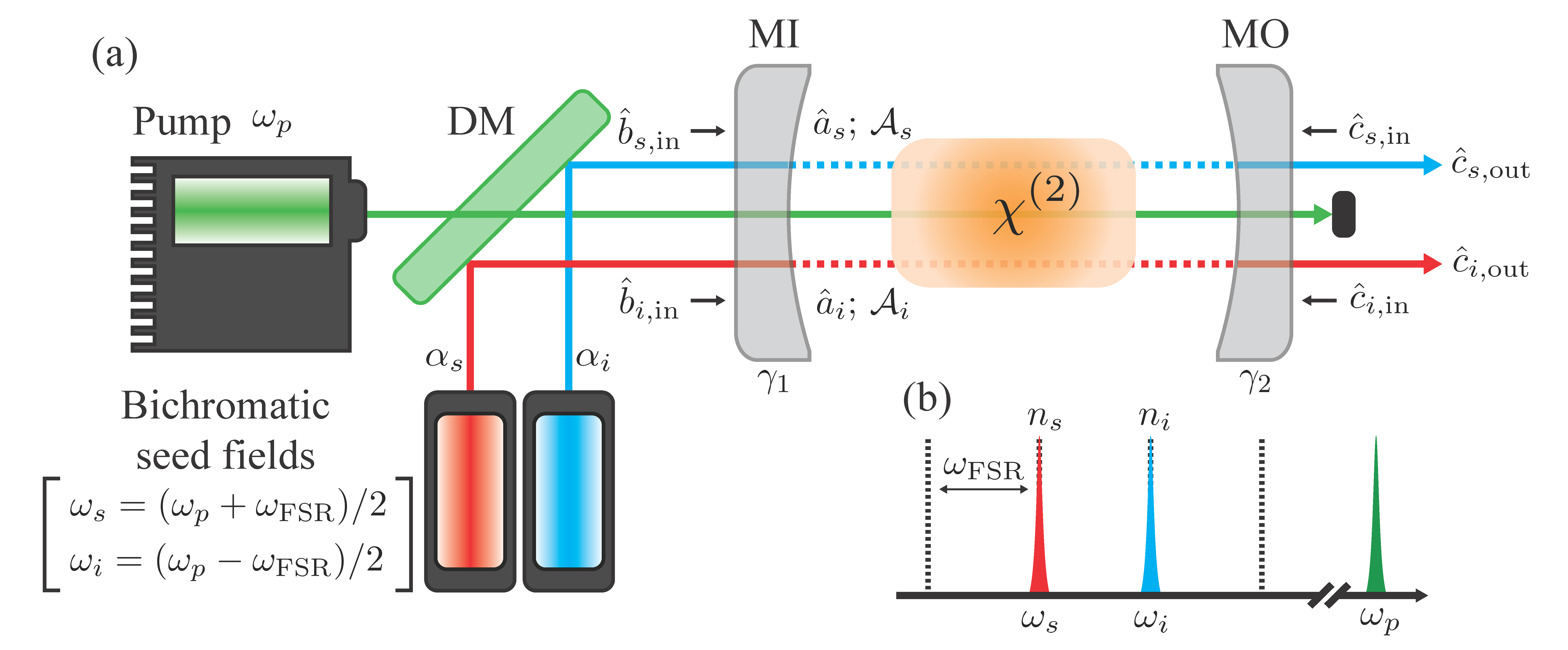
Figure 1(a) shows the schematic diagram of a model system to generate a two-mode stabilized squeezed coherent state (SSCS), . A nonresonant pump laser (green color, frequency , phase at the input mirror) interacts parametrically with the nonlinear crystal located within the OPO cavity to create a pair of nondegenerate two photons in the signal and idler modes via the SPDC process. We assume that the created signal (dotted red color) and idler (dotted blue color) photons are associated with intra-cavity photon annihilation operators and , respectively, and their frequencies are exactly same as the longitudinal mode frequencies with the same polarization, e.g., using a type-0 phase-matching crystal, at and as shown in Fig. 1(b). The optical spectra of the signal mode (mode number ) and idler mode (mode number ) are separated symmetrically by /2 with respect to , i.e., their center frequency is exactly given by , where the pump frequency for intra-cavity SPDC process is (green color) and is free spectral range of cavity.
A phase-matched bichromatic seed field (BSF), i.e., signal and idler seed field with a complex amplitude , couples into the OPO cavity through the input mirror (MI) with the same decay rate , resulting in the intra-cavity injection parameter for signal and idler modes in the interaction picture as , where is the interaction time. In addition, two-mode vacuum fields with input operators and couple into the two cavity modes through the same MI. Moreover, vacuum fields with input operators and couple into the OPO cavity through the output mirror (MO) with decay rate . At the same time, the generated two-mode SSCS field output through the same MO with output operators and , respectively. Thus, in our bichromatic seeding method (BSM), we assume that two-mode SSCS is generated by the stimulated PDC process at the pump non-depletion limit, i.e., well below the OPO threshold. The resultant two-mode SSCS field can be easily separated, e.g., by using a mode-filter cavity for bichromatic homodyne detection (see [37, 38]).
The two-mode system Hamiltonian in the interaction picture for the system depicted in Fig. 1, denoted by , can be expressed within the two-mode Hilbert space as
| (1a) | ||||
| (1b) | ||||
| (1c) | ||||
where is the two-mode down conversion Hamiltonian with the pump-field coupling (squeezing) parameter and is the injection Hamiltonian. Here, we assume below threshold condition, i.e., .
Now, we briefly describe the basic stabilization mechanism for the single-mode system Hamiltonian that has both the squeezing and injection Hamiltonians like Eq. (2) below [39, 40, 41, 42]. We consider a single-mode system Hamiltonian as
| (2) |
where is the single-mode squeezing parameter and is the injection parameter. Then, under the unitary transformation with , where is an arbitrary amplitude, the transformed Hamiltonian can be written as
| (3) |
To make the transformed Hamiltonian independent of the first-order bosonic operators in the displaced frame [41], i.e., representing only the squeezing Hamiltonian with the same squeezing rate , we find that the arbitrary displacement should take the coherent amplitude
| (4) |
and, in this frame, the transformed Hamiltonian has the shifted energy .
As demonstrated above, when the system Hamiltonian contains both the squeezing and injection Hamiltonians like Eq. (2), we can transform it unitarily into an effective system Hamiltonian. To uncouple the system Hamiltonian consisting of the coupled intra-cavity bosonic operators appearing in Eq. (1) into the direct sum of two uncoupled system Hamiltonians, we define two commuting bosonic symmetric annihilation operator and anti-symmetric annihilation operator as
| (5) |
We see that , where is the Kronecker delta and . Next, we define the position and momentum quadrature operators as
| (6) |
where , . Note here that our new bosonic operators are equivalent to the relative position and total momentum quadrature operators in [43]. Similarly, we define two injection rates and associated with and as follows and .
Then, the system Hamiltonian in Eq. (1) can be expressed in this transformed frame as . After removing the shifted energy, decomposes into two completely decoupled terms, and , such that
| (7a) | |||||
| (7b) | |||||
| (7c) | |||||
where the effective displacement amplitudes are and , respectively, for each Hamiltonian and . Thus, single-mode squeezing Hamiltonians in Eqs. (7b) and (7c), those are associated with each phase space for , , can be written as
| (8a) | |||||
| (8b) | |||||
In what follows, we discuss the evolution of two uncoupled quantum states from the two-mode vacuum state by the unitary operators formed by two uncoupled Hamiltonians and given in Eq. (8). In the Schödinger picture, the two-mode quantum state after the interaction with the Hamiltonian during time can be written as
| (9) |
where . In the last term of Eq. (9), and are, respectively, quantum states associated with the symmetric operator and anti-symmetric operator and they can be obtained from Eq. (7) as
| (10a) | |||||
| (10b) | |||||
where is the complex squeezing parameter and , , is the single-mode squeezing operator. Note here that the states in Eq. (10) can be interpreted as the unitary-transformed single-mode squeezed states in each phase space associated with the operators . Indeed, the two states and are obtained, respectively, from the single-mode squeezing Hamiltonians in Eqs. (7b) and (7c) by applying the unitary operators and with effective displacements and .
Finally, we want to point out that in Eq. (9) is indeed equivalent quantum state as the displaced squeezed state , where is the two-mode squeezing operator [44, 45]. Here, the amplitudes and are associated with and in Eq. (7) with the Bogoliubov transformation [46]
| (11a) | ||||
| (11b) | ||||
where and . Indeed, with the Bogoliubov transformation in Eq. (11), we can show that with the help of Eq. (10). Even though the two-mode SSCS in Eq. (9) belongs to one of the Gaussian states in the transformed frame with the effective displacements and , respectively, the nonclassicality of the state remains unclear. This is because the system is in a steady state balanced (stabilized) with bichromatic seeding and decaying out of the cavity, which will be discussed in the next section.
III Nonclassical Properties
Two-mode Gaussian state discussed in the previous section has the well-known variance squeezing of one quadrature (anti-squeezing of conjugate quadrature) and non-zero displacement in phase space (see Appendix A). However, it is unclear whether the quantum state has distinct nonclassical correlations compared to the well-known two-mode squeezed vacuum state and provides sufficient two-mode correlations (entanglement) to be useful for quantum measurement experiments. As such, in this section, we shall first investigate the quantum properties [20, 21, 22, 23, 24, 25, 26, 27, 28, 29, 30, 31, 32, 33] of the two-mode SSCS as functions of controllable system parameters by using the nonclassical measures and introduced by Agarwal [28] and Lee [29]. We then introduce a novel nonclassical indicator, , which unveils the contributions of four distinct SOM components. Notably, exhibits not only global phase dependence but also analytically separates these four key components of nonclassicality. Understanding these components is critical for characterizing the quantum-to-classical transition in the stabilized bipartite entangled systems.
III.1 Nonclassical measures and
The Gaussian analysis in Appendix A does not clearly show the effects of the BSF on the nonclassical properties of the two-mode SSCS. Therefore, we need to further clarify the dependence of quantum properties such as nonclassicality on the coherent injection amplitude for given squeezing parameter . Intuitively, however, we may expect that the quantum properties of the two-mode SSCS should exhibit classical field characteristics at higher seed field amplitudes above some critical value. Therefore, we believe that there must be a range of coherent BSF amplitudes, within which the generated two-mode SSCS exhibits clear nonclassical features such as EPR-like quantum correlations.
To address this issue, we first use a nonclassical measure , defined in Eq. (12) below, based on the classical inequality, i.e., the CSI [27, 28]. If the state has a quantum correlation between the signal and idler modes, according to , the CSI must be violated, i.e., . In this section, we use the calculation results for the analytical expressions of the self- and cross-correlation functions obtained from the solutions of quantum Langevin equations for the and , where is the offset frequency from , in the Heisenberg picture (see Appendix A and B).
We define as the nonclassicality measure of intra-cavity fields from the CSI [28, 27] as
| (12) |
where , , are the SOM functions defined in Eqs. (37), (38), and (39) and their analytical expressions are given in Eqs. (42), (43) and (44). Note here that takes the value , and the two-mode coherent state has the value of . Therefore, any quantum state that has the nonclassical measure between may be interpreted as a kind of nonclassical state, i.e., a state that has strong two-mode quantum correlations.
For comprehensive discussions, we also consider a similar nonclassical measure , defined in Eq. (13) below, based on the Murihead inequality [29] as
| (13) |
The nonclassical measure also takes the value , and any nonclassical state ought to have the value between . Note here that if injection parameters are symmetric, i.e., , is equivalent to .
Furthermore, by using the input-output relation, we can obtain the nonclassical measures and of the two-mode SSCS at the output of the OPO cavity. After a lengthy calculation as described in Appendix B, we find the nonclassical measures of the output fields as
| (14) | ||||
| (15) |
where the individual two-mode correlation functions are found to be
| (16) |
The surprising equivalences of and to their intra-cavity counterparts, found in Eqs. (14) and (15), can be understood as follows. Since and all relate to the intra-cavity ones through the input-output relations in Eq. (29), they share a common multiplicative factor of due to passing through the same output mirror MO with decay rate . Consequently, the ratio in Eq. (14) cancels the effects of the output mirror coupling rate , leading to the identical nonclassical measure: and . In other words, the OPO cavity does not enhance or destroy the SOM property of the intra-cavity fields.
On the other hand, we note that the intra-cavity squeezing level has the maximum value of -3 dB corresponding to the squeezing parameter for at OPO threshold [48, 49], where . As contrary to the nonclassical measure, however, the extra-cavity squeezing parameter , which can be enhanced by the OPO cavity, may have the value up to the infinite squeezing [48, 49], and it is given as
| (17) |
where is the two-mode output variance given in Eq. (34) and is the two-mode vacuum variance.
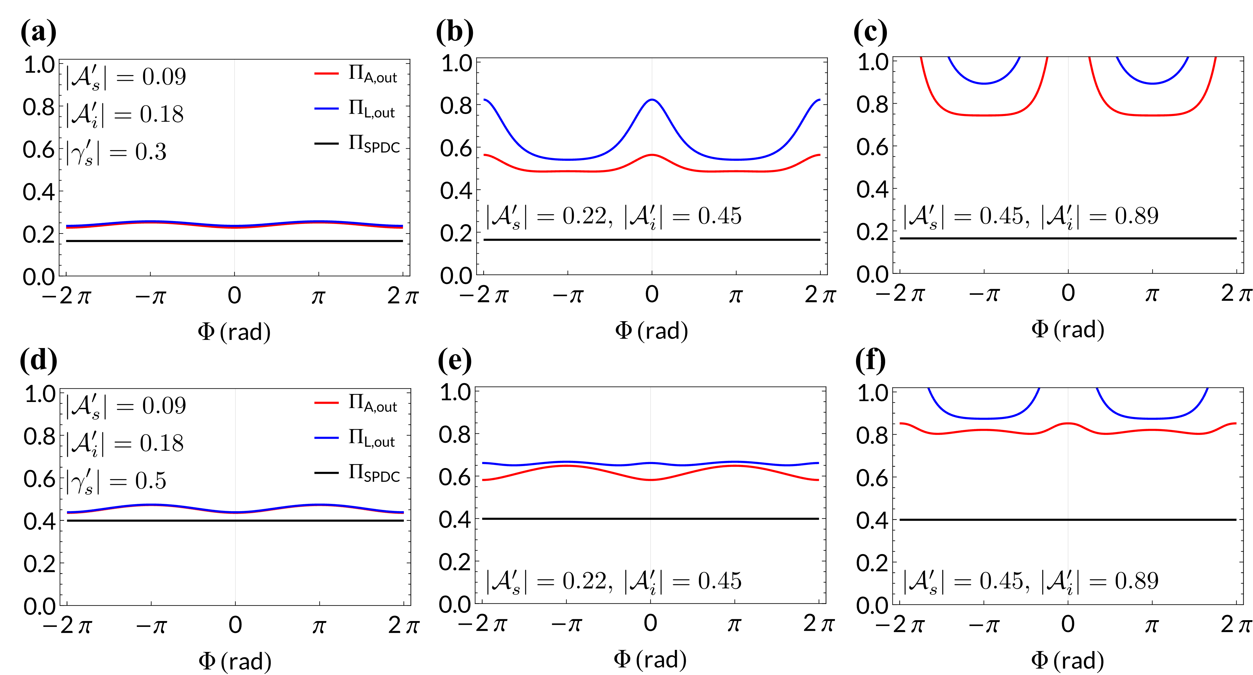
Figure 2 depicts and as a function of the global phase difference for various BSF amplitudes at two different squeezing rates: (low squeezing rate in (a), (b), and (c)) and 0.5 (high squeezing rate in (d), (e), and (f)) with asymmetric injection rates . Here, we used dimensionless parameters such as .
We note here that and for the SPDC process (denoted by ) do not depend on , since in that case there is no bichromatic seed fields, i.e., in , and . Thus, has the minimum value of and at the given squeezing parameter (black solid lines in Fig. 2), and has a very simple expression as
| (18) |
In our BSM presented in Fig. 1, the squeezing rate takes on values in the range . This indicates that our linear model in Eq. (24) operates below the OPO threshold (where ). Consequently, the range of the nonclassical measure falls within 0 and 1. Interestingly, increases monotonically as increases, similar to the observed behavior in the macroscopic coherent regime [31].
In weak seeding regimes in Fig. 2 with and , and exhibit almost the same weak dependence on , reaching their minimum value (maximum nonclassicality) at , for = in panel (a) and 0.5 in panel (d). However, when we increase the seed beam amplitudes to (panel (b) and (e)) and (panel (c) and (f)), and deviate from each other more significantly, and the global phase at which the nonclassical measures have their minimum values changes from to . In these regimes, the system undergo a quantum-to-classical transition much faster at compared to the one at . This behavior can be understood by considering that perfect phase matching of the PDC occurs at , so the coherent seed field is amplified rapidly by the classical frequency conversion (FC) process and reaches the classical boundary easier.
Furthermore, in the intermediate seeding regime (panels (b) and (e)), the nonclassical measures have values still less than 1 for whole range of , confirming that the system exhibits nonclassical quantum correlations at any . However, in the strong seeding regime (panels (c) and (f)), the nonclassical measures exceed 1 at , suggesting that the system has undergone a quantum-to-classical transition at these specific phase values. We also observe that the lower bound of the nonclassical measure approaches 1 (classical) as the squeezing rate approaches the OPO threshold value, . It is interesting to note from our analytical expressions in Eqs. (42), (43) and (44) that and are symmetric with respect to the amplitude ratio of the bichromatic seed fields. Moreover, across all parameter ranges depicted in Fig. 2, consistently exceeds for whole range of . This suggests that can serve as a more sensitive indicator of the quantum-to-classical transition compared to .
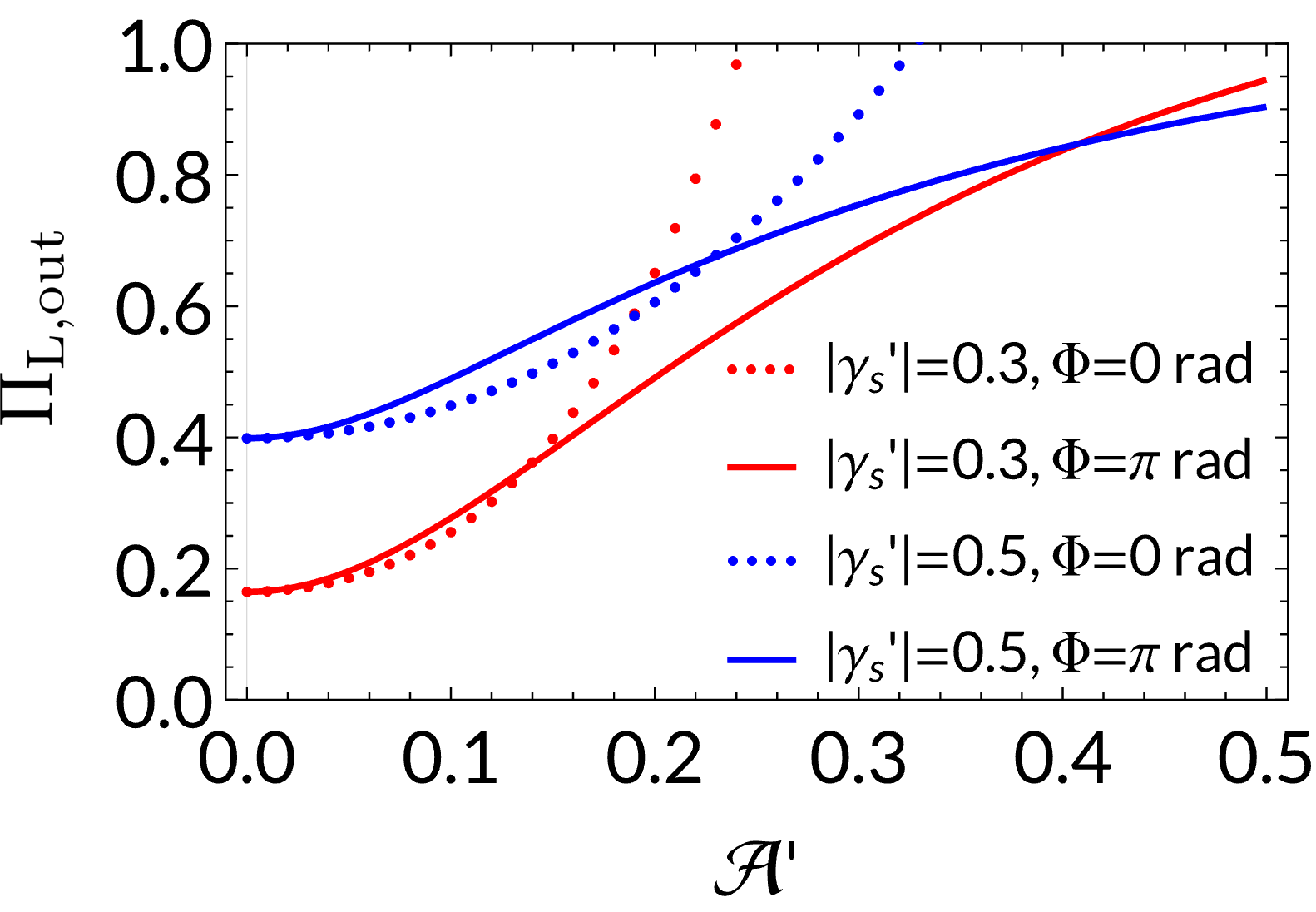
In Fig. 3, we further analyze the dependence of the seed amplitude on at two particular values of and rad plotted against the total injection rate for two different : (red dotted line for and red solid line for rad) and (blue dotted line for and blue solid line for rad). Note here that at and 0.40 for and 0.5, respectively. At perfect phase-matching condition for the PDC process in a nonlinear crystal, i.e., , increases across 1 at for and for as increases from 0. At , however, remains less than 1 as increases up to 0.5 for both values of , confirming the observations in Fig. 2 that at , makes a quantum-to-classical transition faster than at rad as increases from 0. However, it is unclear which process (or system parameter) dictates this quantum-to-classical transition most strongly when controllable system parameters of and are varied.
III.2 Novel nonclassicality indicator
To investigate the effects of each physical process on the nonclassical measure in our BSM, we introduce a novel nonclassical indicator in Eq. (19) below. This measure is derived from the difference between the arithmetic mean and the geometric mean in Eq. (13) as
| (19) |
Then, differs fundamentally from . Unlike which is defined by the ratio of the arithmetic and geometric means, is defined by their difference. This allows to have values outside the 0 to 1 range. A negative value of (i.e., ) indicates nonclassicality of the two-mode state. In this region, the cross-correlation function has a larger value than the self-correlation functions and . In other words, the quantum-to-classical transition occurs at the point where . When the system exhibits predominantly nonclassical properties, will be negative (less than zero). Conversely, for a mostly classical system, will be non-negative (greater than or equal to zero).
In particular, can be decomposed into four individual terms, where each term captures the influence of a specific physical process. Utilizing the notation , we can express as
| (20) |
where , , , and are terms corresponding to each physical process occurring in our BSM in Fig. 1 such as BSF injection, nonlinear FC, SPDC, and StPDC, respectively. In Eq. (20), each term has explicit analytical expressions as
| (21a) | |||
| (21b) | |||
| (21c) | |||
| (21d) | |||
Each term in Eq. (21) has its own physical origin. The first term, always (classicality measure), depends only on the difference between and , i.e., it depends critically on the asymmetry of seeding amplitudes. If , there is no contribution to , meaning has always non-negative contribution to . The second term, always (classicality measure), is proportional to , representing the coherent frequency conversion process with phase-matching factor of . At rad, , thus has always non-negative contribution to . We can now understand the dependence of and in Fig. 2, confirming that at rad, they have more nonclassicality than the case when , and thus the quantum-to-classical transition occurs first at .
The third term, always for (nonclassicality measure), depends only on , indicating that the SPDC process occurs with the parametric pump field alone. Finally, the last term, always (nonclassicality measure) if . This term describes a stimulated single-photon and photon-pair emission processes with the pump and the BSF similar to , but it does not depend on due to the nature of the StPDC process. We want to emphasize that this capacity of revealing contributions of individual physical processes in the nonclassicality measure distinguishes our novel indicator from any previous nonclassical measures.
Many features can be drawn from Eq. (20), since we know analytically the contributions of each term to . Most importantly, the global phase dependence observed in Fig. 2 is due to the contribution of , because it is the only term that depends on . Moreover, is always positive, making the state more classical as the square of the BSF intensity increases. On the other hand, is always negative, and it sets the minimum value of (maximum nonclassicality) when the system operates without the BSF in the below-threshold regime, i.e., , as same as in our BSM. Similarly, always has a negative value and decreases depending on the intensity of the bichromatic seed fields at a given squeezing rate . Lastly, all the contributions from the four distinct physical processes sum up to in Eq. (20), which measures the nonclassicality () of the system with high sensitivity.
As explained above, always has a negative value and is a measure of the nonclassicality of the state without the bichromatic seed fields. In particular, it reaches its minimum value at . Therefore, it is natural to define a normalized nonclassicality indicator, , by dividing in Eq. (20) by as
where , . If we consider the condition of maximum nonclassicality of SPDC process, i.e., , Eq. (III.2) simply reads
| (23) |
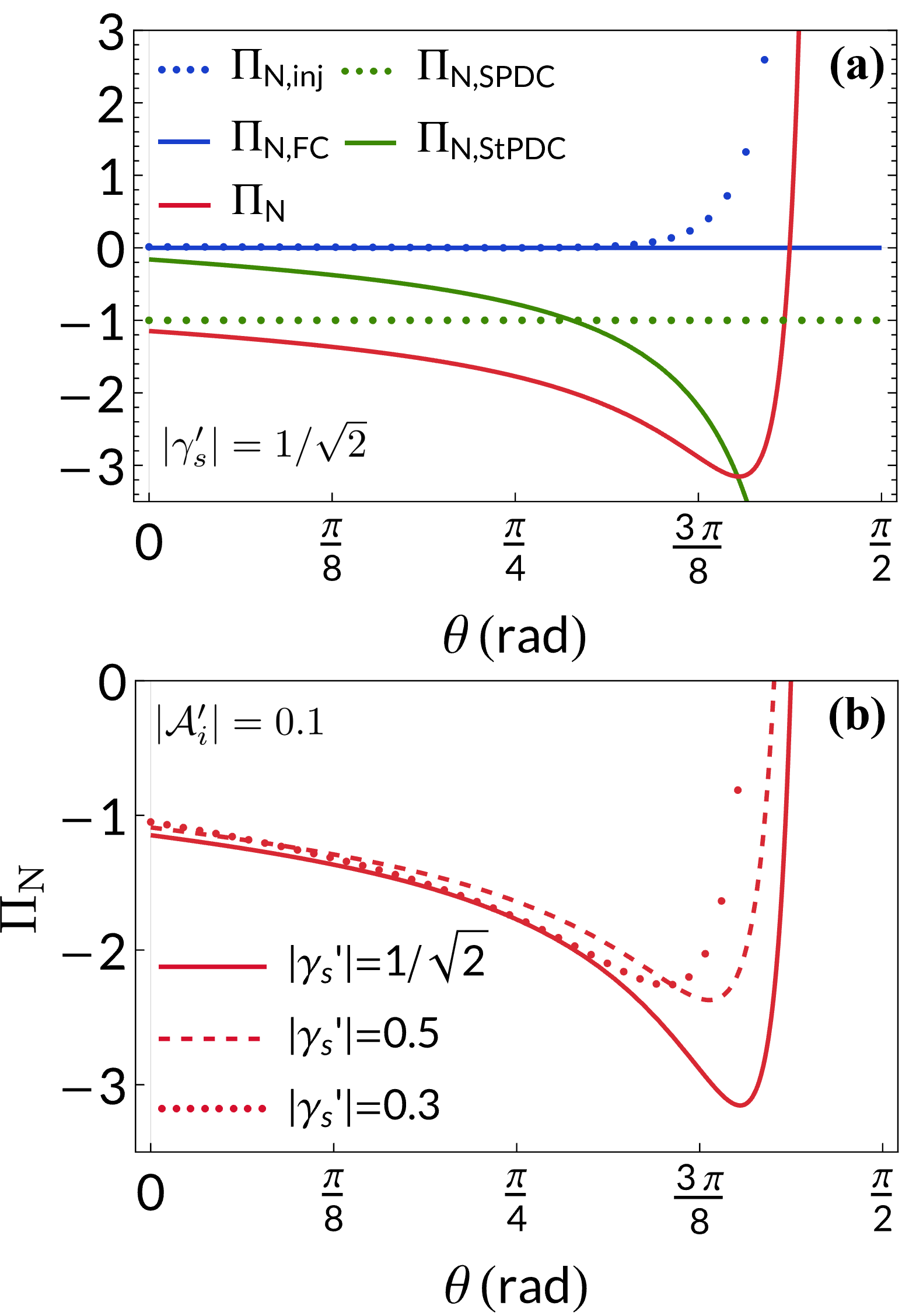
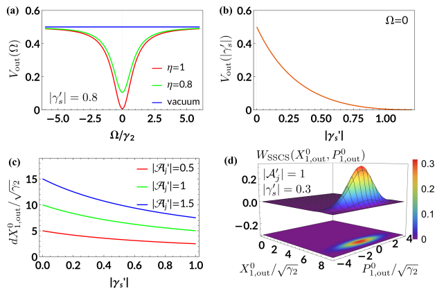
Figure 4(a) depicts the dependence of individual components of in Eq. (III.2) at the phase-mismatch condition, i.e., , on the asymmetric bichromatic seed rate for and : (blue dotted line), (blue solid line), (green dotted line), and (green solid line). (red solid line) is the sum of the four components. At this phase-mismatch condition of , (see Eq. (21b)). Moreover, in Eq. (21a) always has a positive value, while and in Eqs. (21c) and (21d), respectively, have always negative values regardless of the values of squeezing rate and bichromatic seed rates . (red solid line) sums up the four contributions from the four physical processes and it has a minimum negative value (maximum nonclassicality) at rad, since dominates for .
Figure 4(b) shows as a function of for three different squeezing rates: (green solid line), 0.5 (green dashed line), and 0.3 (green dotted line), all for a fixed value of . At the maximum nonclassicality condition of , i.e., , clearly shows the lowest nonclassicality. Specifically, in this high seeding regime ( rad), , which is proportional to as can be seen in Eq. (21a), dominates the other three terms,for three other terms (, and in Eq. (21)) depend mostly on . This dominance by causes of the quantum state to make a quantum-to-classical transition across a value of zero.
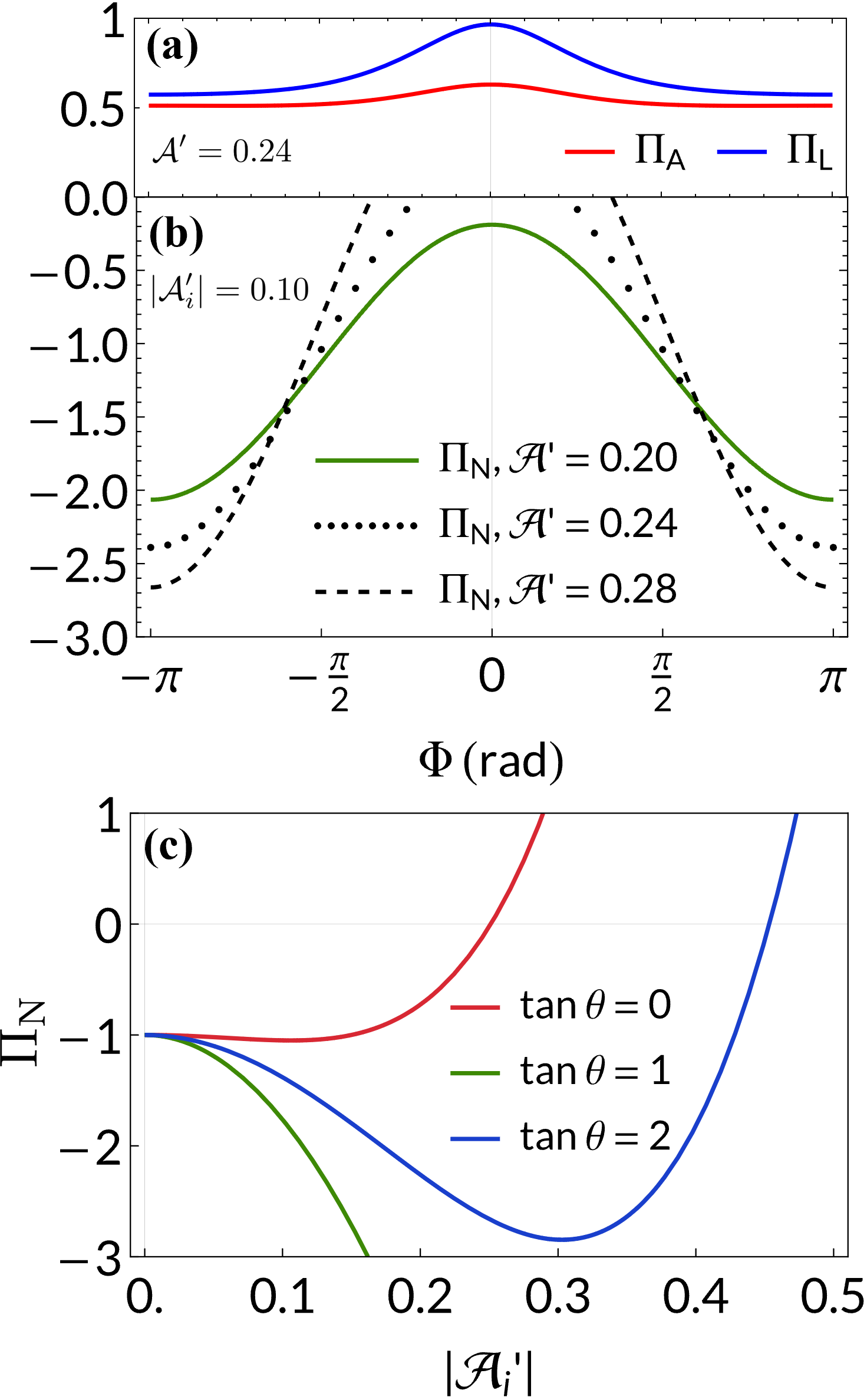
Figure 5 summarizes the parameter dependence of . To compare the sensitivity of on with those of and , we show and versus in Fig. 5(a) at and . In Fig. 5(b), we depict the dependence of on for three different values of : (green solid line), 0.24 (black dotted line), and 0.28 (black dashed line). In all three cases, we fixed the idler seed rate to . In Fig. 5(c), we compare the dependence of on for three different asymmetric seed ratios : (red solid line), i.e., idler seed only, (symmetric seeding, green solid line), and (asymmetric seeding, blue solid line).
When we increase from 0.20 to 0.24 and 0.28 (while fixing the other parameters), shows very similar functional dependence on as those of and as shown in panels (a) and (b). At , they are closer to the border of the quantum-to-classical transition. However, at , they have their minimum possible value due to the effect of as discussed in Fig. 4. For example at (green solid line), still exhibits the nonclassicality of the quantum state for all values of . However, at , at , while and remain in the nonclassical region. This result indicates that our novel measure is more sensitive for determining the nonclassicality of EPR-entangled two-mode squeezed light.
In panel (c), the parameters are fixed at and . We see that even in the case of a single seed beam (red solid line for )), exhibits a broad nonclassical region for , which supports the previously reported observation of single-photon interference in Refs. [50, 51]. Moreover, we also observe that for asymmetric BSF amplitudes, achieves its maximum nonclassicality possible for these fixed system parameters, for example at (blue solid line). We note that one can achieve for the given system parameters in our BSM of Fig. 1 by carefully choosing and perfectly symmetric seeding (green solid line). In this case, however, even slight fluctuations of can force the system to experience quantum-to-classical transition due to the dependence of on .
IV Conclusions and Outlooks
This work investigated nonclassicality criteria for a two-mode stabilized squeezed coherent state (SSCS) of light exhibiting high nonclassicality. The SSCS was generated via an OPO cavity driven by bichromatic weak seed fields. We focused on a quantum system comprising the intra- and extra-cavity fields, operating far below the OPO threshold.
We analyzed first established nonclassicality measures, and , based on the Cauchy-Schwarz and Muirhead inequalities, respectively. Surprisingly, the OPO cavity did not enhance these measures, suggesting that intra-cavity processing does not necessarily improve nonclassicality. Additionally, we found that the global phase difference, , significantly affects these measures. However, for symmetric seeding amplitudes, both and provided equivalent results. For asymmetric seeding, emerged as the more suitable measure.
We then introduced a novel nonclassicality indicator, . This indicator explicitly incorporates four individual terms representing key physical processes: coherent bichromatic injection, nonlinear FC, SPDC, and StPDC. Notably, not only identified the optimal for maximum nonclassicality, aligning with the existing criteria, but also pinpointed the responsible mechanism – the -dependent nonlinear FC process. This highlights ’s ability to reveal previously hidden aspects of nonclassicality.
Our analysis of the parameter dependence of these four components paves the way for studying the quantum-to-classical transition in two-mode entangled systems. Based on the analytical expressions for each component of and numerical simulations, we propose strategies to achieve maximum nonclassicality of the SSCS in the bichromatic seeding method. These strategies involve careful control of the global phase difference (), squeezing rate (), and bichromatic seed amplitudes ( and ) within a weakly-seeded OPO system operating far below threshold.
We anticipate that with advancements in quantum optics techniques, it will be possible to generate two-mode SSCS with a large photon number and a quadrature squeezing parameter exceeding the currently reported value of -15 dB [52]. This paves the way for significant advancements in quantum optics and quantum information science, facilitated by the powerful capabilities of the nonclassicality indicator.
Acknowledgements.
This work was supported by NRF-2022M3K4A109 4781, NRF-2019R1A2C2009974, and NRF-2022K1A3A1 A31091222.Appendix A Two-mode quantum Langevin equation
The quantum Langevin equations of motion for the slowly-varying intra-cavity operators and in the interaction picture with linear approximations [46, 48, 53] can be written as follows:
| (24) |
where is the four-dimensional vector for intra-cavity bosonic slowly-varying operators, and are the four-dimensional vector for slowly-varying input operators associated to the vacuum operators, , and
| (25) |
Here, we used shorthand notations; , , , , and are defined in Sec. II. In addition, we note that the input operators in Eqs. (24) are the input vacuum operators to the signal and idler modes with the dimension of Hz1/2. They enter the OPO cavity through the mirrors MI and MO in Fig. 1 from the outside vacuum with continuous spectra. Equation (24) is derived by the unitary transformation of the intra-cavity Langevin equation for and with the intra-cavity field Hamiltonian in Eq. (1). Equation (24) is valid only in the below-threshold region where . Otherwise, possess eigenvalue with a non-negative real part [39, 40, 42, 53].
Now, to solve the quantum Langevin equation in Eq. (24), we transform the slowly-varying operators into the frequency domain by the Fourier transform around the carrier frequency , such that
| (26) |
We note here that the intra-cavity operators have the physical dimension of Hz-1, and after the Fourier transform, they become dimensionless in the time domain. Then, the solutions of the slowly-varying intra-cavity operators at the signal and idler frequencies can be obtained analytically and summarized as
| (27) |
where and is the Dirac delta function. As one can see, the solutions for and in Eq. (27) are coupled with the vacuum input operators and as well as the coherent amplitudes and . We point out here that the Fourier frequencies and in Eq. (27) are defined within the range of . However, in the calculations below, for simplicity, we shall extend the range of Fourier frequencies up to by considering the narrow linewidth condition of , where is the finesse of the OPO cavity, which can be usually satisfied in quantum optics experiments.
Next, we can use the solutions for and in Eq. (27) to derive the expressions for slowly varying symmetric and antisymmetric operators and in the frequency domain, those are the Fourier transformed operators of and in Eq. (5). We obtained the final expressions as
| (28a) | ||||
| (28b) | ||||
where is the Fourier frequency, , , and .
We stress that the input operators and in Eqs. (28) are vacuum operators that their mean values are zero [53], i.e., . Moreover, since and are mutually independent, we can now investigate the properties of the two-mode squeezed state separately for and .
Next, to investigate the properties of the two-mode squeezed state outside the OPO cavity, we need to find the symmetric and antisymmetric output operators and from the corresponding intra-cavity operators and given in Eq. (28) by using the input-output operator relations [48, 53]
| (29) |
Note here that the first term in the right-hand side of Eq. (29) is the transmitted intra-cavity operator through the output mirror MO of the OPO cavity, and the second one is the input operator reflecting off the output mirror. One can derive the final analytical expressions for and as
| (30a) | ||||
| (30b) | ||||
As a last step, to derive the solutions for the symmetric and antisymmetric position and momentum quadrature operators of the output field from Eq. (30), we will use a simple way introduced in Ref. [48]. Specifically, we define rotated quadrature operators and as the symmetric and antisymmetric position and momentum quadrature operators in the rotated frame. They are rotated by an squeezing angle of from the unrotated frame. In this rotated frame, the symmetric position quadrature operator lies along the semi-major squeezing axis, while the symmetric momentum quadrature operator lies along the semi-minor antisqueezing axis. The antisymmetric quadrature operators exhibit opposite squeezing behavior. Finally, the rotated quadrature operators and can be written as [48]
| (31a) | ||||
| (31b) | ||||
Now, we can easily find the mean values of the position and momentum quadrature operators after the integration over from Eqs. (30) and (31). These are, in fact, the displacements and , respectively, and they depend both on the injection rates and squeezing rate as expected in our BSM as
| (32a) | ||||
| (32b) | ||||
where combinations for and signs in Eq. (32a) and in Eq. (32b) should be applied for to the upper sign pair, and to the lower sign pair, respectively. We want to point out here that in the rotated frame, although the squeezing variance is not dependent on the squeezing angle [48], the expectation values of the symmetric and antisymmetric position and momentum quadrature operators, and equivalently the displacements associated with them, depend on the phase angle , as can be seen in Eqs. (32). We examine these features when we analyze the Wigner functions in Fig. 6 below.
From Eqs. (31) and (32), we can also calculate directly the two-mode squeezing spectrum as well as the two-mode variance , as summarized in Eqs. (33) and (34) below. Note here that, since the constant terms involving in Eqs. (28) are canceled out in their covariances and , the analytical solutions for and depend only on the squeezing parameter .
Finally, we obtained the analytical expression for two-mode squeezing spectrum , which is equal to the normally ordered covariance associated with either the total position quadrature operator or the relative momentum quadrature operator [48, 53] as
| (33) |
where stands for the normal ordering and is the homodyne detection efficiency. As a result, the two-mode squeezing variance can also be obtained by simply adding the two-mode vacuum variance of to the squeezing spectrum as
| (34) |
As clearly seen in Eqs. (33) and (34), the squeezing spectrum and the variance are independent of the bichromatic injection rates and , but depend only on the squeezing parameter . On the other hand, the mean values and in Eqs. (32) depend on both and . Figure 6 summarizes the various Gaussian properties of the SSCS graphically.
Appendix B Calculation of nonclassical properties
To analyze the quantum correlations of the state, we define a second-order moment (SOM) function as
| (35) |
In addition, for two commuting number operators , , and by rearranging the Cauchy-Schwarz inequality, we define a nonclassical measure (Eq. (12)) as the measure of the nonclassicality of the intra-cavity state [28] as
| (36) |
Now, to evaluate the nonclassical measure analytically, we need to calculate the SOM function defined in Eq. (35) by using the expressions of slowly-varying intra-cavity signal and idler operators and in Eq. (27). Then, we can calculate separately each term in the nonclassical measure as follows
| (37) | ||||
| (38) | ||||
| (39) |
where , is the SOM function defined in Eq. (35) with three different combinations of intra-cavity boson operators.
Note here that the slowly varying operators in Eqs. (37) to (39) are actually intra-cavity signal and idler operators with optical frequencies , i.e., , , and . Since we are working in the Heisenberg picture and quantum Langevin equations to study the quantum dynamics of the slowly varying intra-cavity operators and , the SOM functions can be easily evaluated with respect to the two-mode vacuum state after inserting Eq. (27) into Eqs. (37) and (39).
Let’s evaluate some particular term of in Eq. (37). To do this, we need to calculate the expectation values of the product of four intra-cavity signal and idler operators. One can see that has total separate terms of input operators and coherent seed amplitudes. Among them, due to the fact that input annihilation operators have zero eigenvalues for the two-mode vacuum state, expectation values of the terms that have any input annihilation operator at the rightmost place automatically vanishes, resulting in non-zero expectation values from only the terms that have even number of input operators, i.e., from the orthogonality of the number states. Indeed, we have identified that there are only 15 terms in and as well as 17 terms in that have non-zero contributions, including four pairs of 2 isomorphic terms in and with four input operators. We show here only one typical example that has non-zero expectation value, in which one of the creation operator , , is placed at the rightmost place such as
| (40) |
where and .
The expectation value in Eq. (40) can now be simplified by using the bosonic commutation relations such that . Therefore, we can now evaluate simply the four-dimensional (4-D) integration in Eq. (40), resulting in in a very compact form as
| (41) |
It is now straightforward to find the sum of total 15 non-zero terms for and and 17 terms for with the same way as discussed above to obtain Eq. (41). After a lengthy calculation, even though we do not write every result of calculations here, because it takes too many pages and it is hard to gain physical insights from them, we write only the final results for and as well as for the intra-cavity signal and idler modes. The final expressions for , , and may be, respectively, summarized as
| (42) | ||||
| (43) | ||||
| (44) |
where
| (45) | ||||
| (46) |
and and are the coherent amplitudes of the signal and idler seed fields.
Finally, by using the input-output relation, we can obtain the expression for the non-classical measure of the two-mode SSCS at the output of the OPO cavity following the exactly same procedure. After a lengthy calculation, we found a very simple result as
| (47) |
where individual SOM functions are found to be
| (48) |
| (49) |
| (50) |
References
- Furusawa et al. [1998] A. Furusawa, J. L. Sørensen, S. L. Braunstein, C. A. Fuchs, H. J. Kimble, and E. S. Polzik, Unconditional quantum teleportation, Science 282, 706 (1998).
- Braunstein and van Loock [2005] S. L. Braunstein and P. van Loock, Quantum information with continuous variables, Rev. Mod. Phys. 77, 513 (2005).
- Menicucci et al. [2006] N. C. Menicucci, P. van Loock, M. Gu, C. Weedbrook, T. C. Ralph, and M. A. Nielsen, Universal quantum computation with continuous-variable cluster states, Phys. Rev. Lett. 97, 110501 (2006).
- Yadin et al. [2018] B. Yadin, F. C. Binder, J. Thompson, V. Narasimhachar, M. Gu, and M. S. Kim, Operational resource theory of continuous-variable nonclassicality, Phys. Rev. X 8, 041038 (2018).
- Kwon et al. [2019] H. Kwon, K. C. Tan, T. Volkoff, and H. Jeong, Nonclassicality as a quantifiable resource for quantum metrology, Phys. Rev. Lett. 122, 040503 (2019).
- Oelker et al. [2016] E. Oelker, G. Mansell, M. Tse, J. Miller, F. Matichard, L. Barsotti, P. Fritschel, D. E. McClelland, M. Evans, and N. Mavalvala, Ultra-low phase noise squeezed vacuum source for gravitational wave detectors, Optica 3, 682 (2016).
- Ge et al. [2020] W. Ge, K. Jacobs, S. Asiri, M. Foss-Feig, and M. S. Zubairy, Operational resource theory of nonclassicality via quantum metrology, Phys. Rev. Res. 2, 023400 (2020).
- Korobko et al. [2023] M. Korobko, J. Südbeck, S. Steinlechner, and R. Schnabel, Mitigating quantum decoherence in force sensors by internal squeezing, Phys. Rev. Lett. 131, 143603 (2023).
- Otabe et al. [2024] S. Otabe, W. Usukura, K. Suzuki, K. Komori, Y. Michimura, K.-i. Harada, and K. Somiya, Kerr-enhanced optical spring, Phys. Rev. Lett. 132, 143602 (2024).
- Zurek [2003] W. H. Zurek, Decoherence, einselection, and the quantum origins of the classical, Rev. Mod. Phys. 75, 715 (2003).
- Zavatta et al. [2004] A. Zavatta, S. Viciani, and Marco Bellini, Quantum-to-classical transition with single-photon-added coherent states of light, Science 306, 660 (2004).
- Sch [2007] The basic formalism and interpretation of decoherence, in Decoherence and the Quantum-to-Classical Transition (Springer Berlin Heidelberg, Berlin, Heidelberg, 2007) pp. 13–114.
- Rivas and Luis [2010] Á. Rivas and A. Luis, Precision quantum metrology and nonclassicality in linear and nonlinear detection schemes, Phys. Rev. Lett. 105, 010403 (2010).
- Tan et al. [2017] K. C. Tan, T. Volkoff, H. Kwon, and H. Jeong, Quantifying the coherence between coherent states, Phys. Rev. Lett. 119, 190405 (2017).
- Asbóth et al. [2005] J. K. Asbóth, J. Calsamiglia, and H. Ritsch, Computable measure of nonclassicality for light, Phys. Rev. Lett. 94, 173602 (2005).
- Hillery [1987] M. Hillery, Nonclassical distance in quantum optics, Phys. Rev. A 35, 725 (1987).
- Marian et al. [2002] P. Marian, T. A. Marian, and H. Scutaru, Quantifying nonclassicality of one-mode gaussian states of the radiation field, Phys. Rev. Lett. 88, 153601 (2002).
- Lee [1991] C. T. Lee, Measure of the nonclassicality of nonclassical states, Phys. Rev. A 44, R2775 (1991).
- Gehrke et al. [2012] C. Gehrke, J. Sperling, and W. Vogel, Quantification of nonclassicality, Phys. Rev. A 86, 052118 (2012).
- Cabello et al. [2013] A. Cabello, P. Badzia̧g, M. Terra Cunha, and M. Bourennane, Simple Hardy-Like Proof of Quantum Contextuality, Phys. Rev. Lett. 111, 180404 (2013).
- Shafiee et al. [2024] F. H. Shafiee, O. Mahmoudi, R. Nouroozi, and A. Asadian, Nonclassicality of induced coherence witnessed by quantum contextuality, Phys. Rev. A 109, 022216 (2024).
- Vogel and Sperling [2014] W. Vogel and J. Sperling, Unified quantification of nonclassicality and entanglement, Phys. Rev. A 89, 052302 (2014).
- Sperling and Vogel [2009] J. Sperling and W. Vogel, Representation of entanglement by negative quasiprobabilities, Phys. Rev. A 79, 042337 (2009).
- Kiesel et al. [2011] T. Kiesel, W. Vogel, M. Bellini, and A. Zavatta, Nonclassicality quasiprobability of single-photon-added thermal states, Phys. Rev. A 83, 032116 (2011).
- Rahimi-Keshari et al. [2013] S. Rahimi-Keshari, T. Kiesel, W. Vogel, S. Grandi, A. Zavatta, and M. Bellini, Quantum process nonclassicality, Phys. Rev. Lett. 110, 160401 (2013).
- Tan et al. [2020] K. C. Tan, S. Choi, and H. Jeong, Negativity of quasiprobability distributions as a measure of nonclassicality, Phys. Rev. Lett. 124, 110404 (2020).
- Reid and Walls [1986] M. D. Reid and D. F. Walls, Violations of classical inequalities in quantum optics, Phys. Rev. A 34, 1260 (1986).
- Agarwal [1988] G. S. Agarwal, Nonclassical statistics of fields in pair coherent states, J. Opt. Soc. Am. B 5, 1940 (1988).
- Lee [1990a] C. T. Lee, General criteria for nonclassical photon statistics in multimode radiations, Opt. Lett. 15, 1386 (1990a).
- Yong-qing Li et al. [2000] Yong-qing Li, Paul J Edwards, Xu Huang, and Yuzhu Wang, Violation of a classical Cauchy-Schwarz inequality in photon noise spectra, J. Opt. B: Quantum Semiclass. Opt. 2, 292 (2000).
- Marino et al. [2008] A. M. Marino, V. Boyer, and P. D. Lett, Violation of the cauchy-schwarz inequality in the macroscopic regime, Phys. Rev. Lett. 100, 233601 (2008).
- Wasak et al. [2014] T. Wasak, P. Szańńkowski, P. Zińń, M. Trippenbach, and J. Chwedeńńczuk, Cauchy-Schwarz inequality and particle entanglement, Phys. Rev. A 90, 033616 (2014).
- Volovich [2016] I. V. Volovich, Cauchy–Schwarz inequality-based criteria for the non-classicality of sub-Poisson and antibunched light, Phys. Lett. A 380, 56 (2016).
- Glauber [1963] R. J. Glauber, Coherent and incoherent states of the radiation field, Phys. Rev. 131, 2766 (1963).
- Titulaer and Glauber [1965] U. M. Titulaer and R. J. Glauber, Correlation functions for coherent fields, Phys. Rev. 140, B676 (1965).
- Sudarshan [1963] E. C. G. Sudarshan, Equivalence of semiclassical and quantum mechanical descriptions of statistical light beams, Phys. Rev. Lett. 10, 277 (1963).
- Marino et al. [2007] A. M. Marino, Jr. C. R. Stroud, V. Wong, R. S. Bennink, and R. W. Boyd, Bichromatic local oscillator for detection of two-mode squeezed states of light, J. Opt. Soc. Am. B 24, 335 (2007).
- Tian et al. [2020] L. Tian, S.-P. Shi, Y.-H. Tian, Y.-J. Wang, Y.-H. Zheng, and K.-C. Peng, Resource reduction for simultaneous generation of two types of continuous variable nonclassical states, Front. Phys. 16, 21502 (2020).
- Coutinho dos Santos et al. [2005] B. Coutinho dos Santos, K. Dechoum, A. Z. Khoury, L. F. da Silva, and M. K. Olsen, Quantum analysis of the nondegenerate optical parametric oscillator with injected signal, Phys. Rev. A 72, 033820 (2005).
- Golubeva et al. [2008] T. Golubeva, Yu. Golubev, C. Fabre, and N. Treps, Quantum state of an injected TROPO above threshold: Purity,Glauber function and photon number distribution, Eur. Phys. J. D 46, 179 (2008).
- Puri et al. [2017] S. Puri, S. Boutin, and A. Blais, Engineering the quantum states of light in a Kerr-nonlinear resonator by two-photon driving, npj Quantum Inform. 3, 18 (2017).
- Ruiz-Rivas et al. [2018] J. Ruiz-Rivas, G. J. de Valcárcel, and C. Navarrete-Benlloch, Active locking and entanglement in type II optical parametric oscillators, New J. Phys. 20, 023004 (2018).
- Hong-yi and Klauder [1994] F. Hong-yi and J. R. Klauder, Eigenvectors of two particles’ relative position and total momentum, Phys. Rev. A 49, 704 (1994).
- Birrittella et al. [2015] R. Birrittella, A. Gura, and C. C. Gerry, Coherently stimulated parametric down-conversion, phase effects, and quantum-optical interferometry, Phys. Rev. A 91, 053801 (2015).
- Birrittella et al. [2020] R. J. Birrittella, P. M. Alsing, and C. C. Gerry, Phase effects in coherently stimulated down-conversion with a quantized pump field, Phys. Rev. A 101, 013813 (2020).
- Lee and Yoon [2024] C. Lee and T. H. Yoon, Stabilized two-mode squeezed coherent state of light, Optica Open 10.1364/opticaopen.24963987.v1 (2024).
- Lee [1990b] C. T. Lee, Nonclassical photon statistics of two-mode squeezed states, Phys. Rev. A 42, 1608 (1990b).
- Collett and Gardiner [1984] M. J. Collett and C. W. Gardiner, Squeezing of intracavity and traveling-wave light fields produced in parametric amplification, Phys. Rev. A 30, 1386 (1984).
- Qin et al. [2022] W. Qin, A. Miranowicz, and F. Nori, Beating the 3 dB limit for intracavity squeezing and its application to nondemolition qubit readout, Phys. Rev. Lett. 129, 123602 (2022).
- Lee et al. [2018] S. K. Lee, N. S. Han, T. H. Yoon, and M. Cho, Frequency comb single-photon interferometry, Commun. Phys. 1, 51 (2018).
- Yoon and Minhaeng Cho [2021] T. H. Yoon and Minhaeng Cho, Quantitative complementarity of wave-particle duality, Sci. Adv. 7, eabi9268 (2021).
- Vahlbruch et al. [2016] H. Vahlbruch, M. Mehmet, K. Danzmann, and R. Schnabel, Detection of 15 dB squeezed states of light and their application for the absolute calibration of photoelectric quantum efficiency, Phys. Rev. Lett. 117, 110801 (2016).
- Navarrete-Benlloch [2022] C. Navarrete-Benlloch, Introduction to quantum optics (2022), arxiv:2203.13206 [quant-ph] .