Stability, convergence, and pressure-robustness of numerical schemes for incompressible flows with hybrid velocity and pressure

Abstract

In this work we study the stability, convergence, and pressure-robustness of discretization methods for incompressible flows with hybrid velocity and pressure. Specifically, focusing on the Stokes problem, we identify a set of assumptions that yield inf-sup stability as well as error estimates which distinguish the velocity- and pressure-related contributions to the error. We additionally identify the key properties under which the pressure-related contributions vanish in the estimate of the velocity, thus leading to pressure-robustness. Several examples of existing and new schemes that fit into the framework are provided, and extensive numerical validation of the theoretical properties is provided.
Key words: Hybrid approximation methods, Hybrid-High Order methods, Hybridizable Discontinuous Galerkin methods, Inf-sup stability, Presure-robustness
MSC 2010: 65N30, 65N12, 35Q30, 76D07

1 Introduction

In this paper we study the stability, convergence, and pressure-robustness of discretization methods for incompressible flows with hybrid velocity and pressure. Specifically, focusing on the Stokes problem, we identify a set of assumptions that yield (standard or generalized) inf-sup stability as well as error estimates which distinguish the velocity- and pressure-related contributions to the error. We additionally identify the key properties under which the pressure-related contributions vanish in the estimate of the velocity, thus leading to pressure-robustness in the sense of [34]. Several examples of existing and new schemes that fit into the framework are provided.

The use of hybrid approximations of the velocity and discontinuous approximations of the pressure in the context of finite element approximations of incompressible flows dates back to the seminal contribution of Crouzeix and Raviart [19]. Combined with ideas originating from Discontinuous Galerkin methods, this approach later gave rise to a variety of methods [10], including Hybridizable Discontinuous Galerkin methods [32, 16, 17, 14], Hybrid High-Order (HHO) methods [1, 25, 8, 20] and nonconforming Virtual Element methods [2, 37]. More recently, some authors have pointed out the interest of combining hybrid approximations of both the velocity and pressure [35, 28, 7, 3], as this can lead to methods that yield $H(\operatorname{div})$-conforming approximations of the velocity and possibly exhibit a better behaviour in the quasi-inviscid limit.

The goal of the present work is precisely to provide a rigorous framework of analysis for such methods focusing on the Stokes problem. To this purpose, we use as a starting point a fully discrete presentation closely inspired by HHO methods and the Third Strang Lemma of [21]. The discrete pressure-velocity coupling hinges on local reconstructions of the velocity divergence and the pressure gradient obtained mimicking integration by parts formulas. The key to the discretization of the viscous term are, on the other hand, a velocity gradient and a stabilization bilinear form. The description of the scheme is completed by prescribing a velocity interpolator at elements. Starting from an abstract scheme based on the above ingredients, we identify inclusion relations of the local pressure spaces into the local velocity spaces that guarantee stability in the form of a generalized inf-sup condition. A standard inf-sup condition is recovered when the discrete velocity divergence and pressure gradient satisfy a global discrete integration by parts formula for interpolates of smooth velocity fields. Under proper choices of discrete spaces and operators, we derive error estimates that distinguish the velocity- and pressure-contributions to the error. Such error estimates turn out to be pressure-robust when standard inf-sup stability holds, as well as suitable inclusion relations between the local velocity and pressure spaces. This abstract framework is applied to derive new pressure-robust error estimates for the classical Botti–Massa scheme of [7]. A similar analysis of the Rhebergen–Wells method of [35] is also carried out, providing alternative proofs of the findings of [28]. Finally, new schemes are also identified and analyzed, both on standard and polyhedral meshes, and extensive numerical validation of the theoretical properties is provided.

The importance of deriving velocity error estimates independent of the pressure has been pointed out in several works; see, e.g., [33, 31, 30]. A classical strategy for achieving pressure-robustness consists in using stable mixed methods with $H(\operatorname{div})$-conforming and divergence-free approximate velocities [27]. This strategy has been, in particular, pursued in the context of Discontinuous Galerkin methods [18, 36, 29]. Recently, it has also been suggested in [30, 29] that pressure-robust techniques can be used to remedy the suboptimal approximation results for non-Newtonian Stokes problems [5, 9]. Pressure-robust methods supporting general polyhedral meshes and based on local $H(\operatorname{div})$-conforming reconstructions on simplicial submeshes have been explored, e.g., in [26, 13]. Recent works have also pointed out that pressure-robustness on polytopal meshes can be achieved without using a submesh when compatible approximation of the curl-curl formulation of the Navier–Stokes equations are used [4, 23].

The rest of this paper is organized as follows. In Section 2 we set the stage of the paper by introducing hybrid spaces, interpolators, and reconstructions of quantities in terms of the hybrid unknowns. In Section 3 we state an abstract discretization method for the Stokes problem and prove (generalized) inf-sup stability of the pressure-velocity coupling. A full stability and convergence analysis of the scheme is provided in Section 4. Applications of the framework to existing and new schemes are considered in Section 5. Finally, a numerical assessment of the predicted convergence rates and pressure-robustness properties is provided in Section 6.

2 Hybrid spaces, interpolators, and reconstructions

2.1 Mesh and notation for inequalities

Let $\Omega\subset\mathbb{R}^{d}$, $d\geq 1$, denote an open bounded polytopal domain. Denote by $\mathcal{M}_{h}=(\mathcal{T}_{h},\mathcal{F}_{h})$ a mesh of the domain $\Omega$ in the sense of [22, Chapter 1], with $\mathcal{T}_{h}$ collecting the mesh elements and $\mathcal{F}_{h}$ the mesh faces. Notice that the term faces refers to (hyper-)planar portions of the element boundaries, i.e., faces when $d=3$, edges when $d=2$. Additional assumptions on the shape of the elements may be needed for specific methods in Section 5. The set of faces is partitioned into the sets $\mathcal{F}_{h}^{\rm i}$ of internal faces and $\mathcal{F}_{h}^{\rm b}$ of boundary faces. For each mesh element $T\in\mathcal{T}_{h}$, we denote by $\mathcal{F}_{T}$ the set of faces that lie on its boundary $\partial T$ and, for any $F\in\mathcal{F}_{T}$, we denote by $n_{TF}$ the unit vector normal to $F$ pointing out of $T$. For each internal face $F\in\mathcal{F}_{h}^{\rm i}$, we additionally fix once and for all an orientation through the unit normal vector $n_{F}$. For boundary faces, we select $n_{F}$ pointing out of $\Omega$.

When stating convergence results, we assume that $\mathcal{M}_{h}$ belongs to a sequence of refined meshes indexed by the mesh size $h$. Inequalities that hold up to a multiplicative constant independent of $h$ are denoted with the $\lesssim$ sign, and we furthermore write $a\simeq b$ in place of “$a\lesssim b$ and $b\lesssim a$”.

2.2 Hybrid velocity and pressure spaces

We consider methods where the velocity and pressure are both approximated using hybrid spaces, i.e., spaces spanned by vectors of local functions attached to both element and faces:

$$\underline{U}_{h}\coloneq\left(\bigtimes_{T\in\mathcal{T}_{h}}U_{T}\right)\times\left(\bigtimes_{F\in\mathcal{F}_{h}}U_{F}\right),\qquad\underline{P}_{h}\coloneq\left(\bigtimes_{T\in\mathcal{T}_{h}}P_{T}\right)\times\left(\bigtimes_{F\in\mathcal{F}_{h}}P_{F}\right),$$

where $U_{T}\subset L^{2}(T)^{d}$ and $P_{T}\subset L^{2}(T)$ for all $T\in\mathcal{T}_{h}$ with $P_{T}$ containing at least constant functions on $T$, while $U_{F}\subset L^{2}(F)^{d}$ and $P_{F}\subset L^{2}(F)$ for all $F\in\mathcal{F}_{h}$. Following standard conventions in the framework of fully discrete methods, we denote the restrictions of the above spaces and their elements to a mesh element $T\in\mathcal{T}_{h}$ by replacing the subscript $h$ with $T$.

2.3 Interpolators and projectors

We denote by $I_{U,T}:H^{1}(T)^{d}\to U_{T}$ the interpolator onto $U_{T}$ and by $I_{U,F}:L^{2}(F)^{d}\to U_{F}$ the $L^{2}$-orthogonal projector onto $U_{F}$, and set, for all $v\in H^{1}(\Omega)^{3}$,

$$\underline{I}_{U,h}v\coloneq\big{(}(I_{U,T}v)_{T\in\mathcal{T}_{h}},(I_{U,F}v)_{F\in\mathcal{F}_{h}}\big{)}.$$

Similarly, we denote by $I_{P,Y}:L^{2}(Y)\to P_{Y}$, $Y\in\mathcal{T}_{h}\cup\mathcal{F}_{h}$, the $L^{2}$-orthogonal projector onto $P_{Y}$ and set, for all $q\in H^{1}(\Omega)$,

$$\underline{I}_{P,h}q\coloneq\big{(}(I_{P,T}q)_{T\in\mathcal{T}_{h}},(I_{P,F}q)_{F\in\mathcal{F}_{h}}\big{)}.$$

Notice that, while $I_{U,F}$, $I_{P,T}$, and $I_{P,F}$ are all $L^{2}$-orthogonal projectors, we leave more freedom for $I_{U,T}$, as it will be needed in the analysis of certain methods in Section 5. Specifically, we only make the following continuity requirement: For all $v\in H_{0}^{1}(\Omega)^{d}$,

$$\|\underline{I}_{U,h}v\|_{1,h}\lesssim\|v\|_{H^{1}(\Omega)^{d}},$$ (1)

where the $H^{1}$-like seminorm $\|\cdot\|_{1,h}$ on $\underline{U}_{h}$ is such that, for all $\underline{v}_{h}\in\underline{U}_{h}$,

$$\begin{gathered}\|\underline{v}_{h}\|_{1,h}^{2}\coloneq\sum_{T\in\mathcal{T}_{h}}\|\underline{v}_{T}\|_{1,T}^{2}\\ \text{with $\|\underline{v}_{T}\|_{1,T}^{2}\coloneq\|\nabla v_{T}\|_{L^{2}(T)^{d\times d}}^{2}+h_{T}^{-1}\sum_{F\in\mathcal{F}_{T}}\|v_{F}-v_{T}\|_{L^{2}(F)^{d}}^{2}$ for all $T\in\mathcal{T}_{h}$. }\end{gathered}$$ (2)

The $L^{2}$-orthogonal projector on a space $X$ different from the component spaces will be denoted by $\pi_{X}$.

2.4 Discrete velocity divergence

Let the discrete velocity divergence $D_{T}:\underline{U}_{T}\to P_{T}$ be such that, for all $\underline{v}_{T}\in\underline{U}_{T}$,

$$\int_{T}D_{T}\underline{v}_{T}\,q_{T}=-\int_{T}v_{T}\cdot\nabla q_{T}+\sum_{F\in\mathcal{F}_{T}}\int_{F}(v_{F}\cdot n_{TF})\,q_{T}\qquad\forall q_{T}\in P_{T}.$$ (3)

Assumption 1.

For all $T\in\mathcal{T}_{h}$, it holds

1. $\nabla P_{T}\subset U_{T}$ and $\pi_{\nabla P_{T}}\circ I_{U,T}=\pi_{\nabla P_{T}}$ with $\pi_{\nabla P_{T}}$ $L^{2}$-orthogonal projector onto $\nabla P_{T}$;

2. $\operatorname{tr}_{F}P_{T}\subset U_{F}\cdot n_{TF}$ for all $F\in\mathcal{F}_{T}$.

Proposition 1 (Commutativity of $D_{T}$).

Under Assumption 1 we have, for all $v\in H^{1}(T)^{d}$,

$$D_{T}\underline{I}_{U,T}v=I_{P,T}(\nabla\cdot v).$$ (4)

Proof.

Apply the definition (3) of $D_{T}$ to $\underline{v}_{T}=\underline{I}_{U,T}v$, notice that, by Assumption 1, $I_{U,T}$ and $I_{U,F}$ can be cancelled from the right-hand side, and integrate the latter by parts. ∎

2.5 Discrete pressure gradient

We next define the pressure gradient $G_{T}:\underline{P}_{T}\to U_{T}$ such that, for all $\underline{q}_{T}\in\underline{P}_{T}$,

$$\int_{T}G_{T}\underline{q}_{T}\cdot v_{T}=-\int_{T}q_{T}\,(\nabla\cdot v_{T})+\sum_{F\in\mathcal{F}_{T}}\int_{F}q_{F}\,(v_{T}\cdot n_{TF})\qquad\forall v_{T}\in U_{T}.$$ (5)

Assumption 2.

For all $T\in\mathcal{T}_{h}$, it holds

1. $\nabla\cdot U_{T}\subset P_{T}$;

2. $U_{F}\cdot n_{TF}\subset P_{F}$ for all $F\in\mathcal{F}_{T}$.

The proof of the following result is analogous to that of Proposition 1.

Proposition 2 (Commutativity of $G_{T}$).

Under Assumption 2 we have, for all $T\in\mathcal{T}_{h}$ and all $q\in H^{1}(T)$,

$$G_{T}\underline{I}_{P,T}q=\pi_{U_{T}}(\nabla q).$$ (6)

For future use we note the following formula, which establishes a link between the discrete velocity divergence and pressure gradient: For all $(\underline{v}_{T},\underline{q}_{T})\in\underline{U}_{T}\times\underline{P}_{T}$,

$$\int_{T}G_{T}\underline{q}_{T}\cdot v_{T} =\int_{T}\nabla q_{T}\cdot v_{T}+\sum_{F\in\mathcal{F}_{T}}\int_{F}(q_{F}-q_{T})(v_{T}\cdot n_{TF})$$ (7)

$$\overset{\eqref{eq:DT}}{} =-\int_{T}D_{T}\underline{v}_{T}\,q_{T}+\sum_{F\in\mathcal{F}_{T}}\int_{F}(v_{T}-v_{F})\cdot n_{TF}\,(q_{F}-q_{T}),$$

where the equality in the first line is obtained integrating by parts the right-hand side of (5).

3 Hybrid discretizations of the Stokes problem

In this section we formulate an abstract approximation scheme for the Stokes problem: Given $f:\Omega\to\mathbb{R}^{d}$, find $u:\Omega\to\mathbb{R}^{d}$ and $p:\Omega\to\mathbb{R}$ such that

$$-\nu\Delta u+\nabla p =f \text{in $\Omega$},$$ (8)

$$\nabla\cdot u =0 \text{in $\Omega$},$$

$$u =0 \text{on $\partial\Omega$},$$

$$\int_{\Omega}p =0,$$

where $\nu>0$ denotes the kinematic viscosity. Throughout the rest of this work we assume $f\in L^{2}(\Omega)^{d}$ and focus on the standard weak formulation of problem (8) with velocity $u\in H^{1}_{0}(\Omega)^{d}$ and pressure $p\in L^{2}_{0}(\Omega)\coloneq\left\{q\in L^{2}(\Omega)\,:\,\int_{\Omega}q=0\right\}$. The velocity approximation will be sought in the following subspace of $\underline{U}_{h}$ incorporating homogeneous Dirichlet boundary conditions:

$$\underline{U}_{h,0}\coloneq\left\{\big{(}(v_{T})_{T\in\mathcal{T}_{h}},(v_{F})_{F\in\mathcal{F}_{h}}\big{)}\in\underline{U}_{h}\,:\,\text{$v_{F}=0$ for all $F\in\mathcal{F}_{h}^{\rm b}$}\right\}.$$

To define the discrete space for the pressure, for all $\underline{q}_{h}\in\underline{P}_{h}$ we let $q_{h}\in L^{2}(\Omega)$ (not underlined) be such that $(q_{h})_{|T}\coloneq q_{T}$ for all $T\in\mathcal{T}_{h}$ and set

$$\underline{P}_{h,0}\coloneq\left\{\underline{q}_{h}\in\underline{P}_{h}\,:\,\int_{\Omega}q_{h}=0\right\}.$$

3.1 Pressure-velocity coupling

Let $b_{h}:\underline{U}_{h}\times\underline{P}_{h}\to\mathbb{R}$ be such that, for all $(\underline{v}_{h},\underline{q}_{h})\in\underline{U}_{h}\times\underline{P}_{h}$,

$$b_{h}(\underline{v}_{h},\underline{q}_{h})\coloneq\sum_{T\in\mathcal{T}_{h}}b_{T}(\underline{v}_{T},\underline{q}_{T}) b_{T}(\underline{v}_{T},\underline{q}_{T})\coloneq\int_{T}G_{T}\underline{q}_{T}\cdot v_{T}$$ with . (9)

Notice that, by (7), the following equivalent reformulation of $b_{h}$ holds:

$$b_{h}(\underline{v}_{h},\underline{q}_{h})=-\sum_{T\in\mathcal{T}_{h}}\int_{T}D_{T}\underline{v}_{T}\,q_{T}+\sum_{T\in\mathcal{T}_{h}}\sum_{F\in\mathcal{F}_{T}}\int_{F}(v_{T}-v_{F})\cdot n_{TF}\,(q_{F}-q_{T}).$$ (10)

Let us now consider the stability of the pressure-velocity coupling. To this purpose, we define the boundary pressure seminorm $|\cdot|_{0,h}:\underline{P}_{h}\to\mathbb{R}$ such that, for all $\underline{q}_{h}\in\underline{P}_{h}$,

$$|\underline{q}_{h}|_{0,h}^{2}\coloneq\sum_{T\in\mathcal{T}_{h}}|\underline{q}_{T}|_{0,T}^{2} |\underline{q}_{T}|_{0,T}^{2}\coloneq h_{T}\sum_{F\in\mathcal{F}_{T}}\|q_{F}-q_{T}\|_{L^{2}(F)}^{2} T\in\mathcal{T}_{h}$$ with for all . (11)

Assumption 3.

For all $(v,\underline{q}_{h})\in H^{1}(\Omega)^{d}\times\underline{P}_{h}$, it holds

$$\mathcal{E}_{{\rm ibp},h}(v,\underline{q}_{h})\coloneq\sum_{T\in\mathcal{T}_{h}}\sum_{F\in\mathcal{F}_{T}}\int_{F}(I_{U,T}v-I_{U,F}v)\cdot n_{TF}\,(q_{F}-q_{T})=0.$$ (12)

Throughout the rest of the paper, we let

$$\delta\coloneq\begin{cases}0&\text{if Assumption~{}\ref{ass:global.ibp} holds,}\\ 1&\text{otherwise.}\end{cases}$$

Notice that the quantity $\mathcal{E}_{{\rm ibp},h}(v,\underline{q}_{h})$ measures the failure to satisfy a global integration by parts formula, and therefore corresponds a conformity error in the usual finite element terminology.

Lemma 3 (Inf-sup and generalized inf-sup conditions).

Let Assumption 1 hold and set, for all $\underline{q}_{h}\in\underline{P}_{h}$,

$$\|\underline{q}_{h}\|_{{\rm P},h}\coloneq\left(\|q_{h}\|_{L^{2}(\Omega)}^{2}+\sum_{T\in\mathcal{T}_{h}}h_{T}^{2}\|G_{T}\underline{q}_{T}\|_{L^{2}(T)^{d}}^{2}\right)^{\frac{1}{2}}.$$

Then, for all $\underline{q}_{h}\in\underline{P}_{h,0}$, we have the following (generalized) inf-sup condition:

$$\|\underline{q}_{h}\|_{{\rm P},h}\lesssim\sup_{\underline{v}_{h}\in\underline{U}_{h,0}\setminus\{\underline{0}\}}\frac{b_{h}(\underline{v}_{h},\underline{q}_{h})}{\|\underline{v}_{h}\|_{1,h}}+\delta|\underline{q}_{h}|_{0,h},$$ (13)

which reduces to a standard inf-sup condition when Assumption 3 holds.

Proof.

Let $\underline{q}_{h}\in\underline{P}_{h,0}$ and, for the sake of brevity, denote by $\$$ the supremum in the right-hand side of (13). Since $q_{h}\in L^{2}_{0}(\Omega)$, the continuous inf-sup condition yields the existence of

$$v_{q}\in H_{0}^{1}(\Omega)^{d} \nabla\cdot v_{q}=q_{h} \|v_{q}\|_{H^{1}(\Omega)^{d}}\lesssim\|q_{h}\|_{L^{2}(\Omega)}$$ such that and . (14)

Let $\underline{w}_{h}\in\underline{U}_{h}$ be such that $w_{T}=h_{T}^{2}\,G_{T}\underline{q}_{T}$ for all $T\in\mathcal{T}_{h}$ and $w_{F}=0$ for all $F\in\mathcal{F}_{h}$ and notice that, by discrete inverse and trace inequalities,

$$\|\underline{w}_{h}\|_{1,h}\lesssim\left(\sum_{T\in\mathcal{T}_{h}}h_{T}^{2}\|G_{T}\underline{q}_{T}\|_{L^{2}(T)^{d}}^{2}\right)^{\frac{1}{2}}.$$ (15)

We have

$$\|\underline{q}_{h}\|_{{\rm P},h}^{2}\overset{\eqref{eq:continuous.inf-sup},\,\eqref{eq:bh}}{} =\int_{\Omega}(\nabla\cdot v_{q})\,q_{h}+b_{h}(\underline{w}_{h},\underline{q}_{h})$$

$$=\sum_{T\in\mathcal{T}_{h}}\int_{\Omega}I_{P,T}(\nabla\cdot v_{q})\,q_{T}+b_{h}(\underline{w}_{h},\underline{q}_{h})\overset{\eqref{eq:DT:commutativity}}{=}\sum_{T\in\mathcal{T}_{h}}\int_{\Omega}(D_{T}\underline{I}_{U,T}v_{q})\,q_{T}+b_{h}(\underline{w}_{h},\underline{q}_{h})$$

$$\overset{\eqref{eq:bh:bis}}{} =-b_{h}(\underline{I}_{U,h}v_{q},\underline{q}_{h})+\delta\sum_{T\in\mathcal{T}_{h}}\sum_{F\in\mathcal{F}_{T}}\int_{F}(I_{U,T}v_{q}-I_{U,F}v_{q})\cdot n_{TF}\,(q_{F}-q_{T})+b_{h}(\underline{w}_{h},\underline{q}_{h})$$

$$\leq\$\|\underline{I}_{U,h}v_{q}\|_{1,h}+\delta\|\underline{I}_{U,h}v_{q}\|_{1,h}|\underline{q}_{h}|_{0,h}+\$\|\underline{w}_{h}\|_{1,h}$$

$$\overset{\eqref{eq:IUh:continuity}}{} \lesssim\left(\$+\delta|\underline{q}_{h}|_{0,h}\right)\|v_{q}\|_{H^{1}(\Omega)^{d}}+\$\|\underline{w}_{h}\|_{1,h}\overset{\eqref{eq:continuous.inf-sup},\,\eqref{eq:wh:norm.equivalence}}{\lesssim}\left(\$+\delta|\underline{q}_{h}|_{0,h}\right)\|\underline{q}_{h}\|_{{\rm P},h},$$

where, in the first inequality, we have used the definition of supremum for the first and third terms and Cauchy–Schwarz inequalities along with the definitions (2) of $\|\cdot\|_{1,h}$ and (11) of $|\cdot|_{0,h}$ for the second term. Simplifying, the conclusion follows. ∎

3.2 Viscous terms

Let a local space $\Sigma_{T}\subset L^{2}(T)^{d\times d}$ be given. The discretization of the viscous terms is based on the velocity gradient $E_{T}:\underline{U}_{T}\to\Sigma_{T}$ such that, for all $\underline{v}_{T}\in\underline{U}_{T}$ and all $\tau\in\Sigma_{T}$,

$$\int_{T}E_{T}\underline{v}_{T}:\tau =-\int_{T}v_{T}\cdot(\nabla\cdot\tau)+\sum_{F\in\mathcal{F}_{T}}\int_{F}v_{F}\cdot(\tau n_{TF})$$ (16a)

$$=\int_{T}\nabla v_{T}:\tau+\sum_{F\in\mathcal{F}_{T}}\int_{F}(v_{F}-v_{T})\cdot(\tau n_{TF}).$$ (16b)

The space $\Sigma_{T}$ is typically selected in order for the following assumption to hold true.

Assumption 4.

The following holds:

1. $\nabla\cdot\Sigma_{T}\subset U_{T}$ and $\pi_{\nabla\cdot\Sigma_{T}}\circ I_{U,T}=\pi_{\nabla\cdot\Sigma_{T}}$;

2. $\Sigma_{T}n_{TF}\subset U_{F}$ for all $F\in\mathcal{F}_{T}$.

The proof of the following result is analogous to that of Proposition 1.

Proposition 4 (Commutativity of $E_{T}$).

Under Assumption 4, it holds, for all $v\in H^{1}(T)^{d}$,

$$E_{T}\underline{I}_{U,T}v=\pi_{\Sigma_{T}}(\nabla v).$$

We let $a_{h}:\underline{U}_{h}\times\underline{U}_{h}\to\mathbb{R}$ be such that, for all $(\underline{w}_{h},\underline{v}_{h})\in\underline{U}_{h}\times\underline{U}_{h}$,

$$a_{h}(\underline{w}_{h},\underline{v}_{h})\coloneq\sum_{T\in\mathcal{T}_{h}}a_{T}(\underline{w}_{T},\underline{v}_{T}) a_{T}(\underline{w}_{T},\underline{v}_{T})\coloneq\int_{T}E_{T}\underline{w}_{T}:E_{T}\underline{v}_{T}+s_{T}(\underline{w}_{T},\underline{v}_{T})$$ with , (17)

where $s_{T}:\underline{U}_{T}\times\underline{U}_{T}\to\mathbb{R}$ is a (possibly zero) symmetric positive semi-definite stabilization bilinear form.

Assumption 5.

Recalling (2), the following uniform norm equivalence holds:

$$\|\underline{v}_{h}\|_{1,h}\simeq a_{h}(\underline{v}_{h},\underline{v}_{h})^{\frac{1}{2}}\qquad\forall\underline{v}_{h}\in\underline{U}_{h,0}.$$

3.3 An abstract hybrid scheme

We consider the following hybrid discretization of problem (8): Find $(\underline{u}_{h},\underline{p}_{h})\in\underline{U}_{h,0}\times\underline{P}_{h,0}$ such that

$$\nu a_{h}(\underline{u}_{h},\underline{v}_{h})+b_{h}(\underline{v}_{h},\underline{p}_{h}) =\int_{\Omega}f\cdot v_{h} \forall\underline{v}_{h}\in\underline{U}_{h,0},$$ (18)

$$-b_{h}(\underline{u}_{h},\underline{q}_{h})+\delta\nu^{-1}d_{h}(\underline{p}_{h},\underline{q}_{h}) =0 \forall\underline{q}_{h}\in\underline{P}_{h,0},$$

where $v_{h}\in L^{2}(\Omega)^{d}$ (not underlined) is such that $(v_{h})_{|T}\coloneq v_{T}$ for all $T\in\mathcal{T}_{h}$ and the bilinear form $d_{h}:\underline{P}_{h}\times\underline{P}_{h}\to\mathbb{R}$ is such that

$$d_{h}(\underline{p}_{h},\underline{q}_{h})\coloneq\sum_{T\in\mathcal{T}_{h}}d_{T}(\underline{p}_{T},\underline{q}_{T}) d_{T}(\underline{p}_{T},\underline{q}_{T})\coloneq h_{T}\sum_{F\in\mathcal{F}_{T}}\int_{F}(p_{F}-p_{T})\,(q_{F}-q_{T}) T\in\mathcal{T}_{h}$$ with for all .

Defining the bilinear form $\mathcal{A}_{h}:\left[\underline{U}_{h}\times\underline{P}_{h}\right]^{2}\to\mathbb{R}$ such that, for all $((\underline{w}_{h},\underline{r}_{h}),(\underline{v}_{h},\underline{p}_{h}))\in\left[\underline{U}_{h}\times\underline{P}_{h}\right]^{2}$,

$$\mathcal{A}_{h}((\underline{w}_{h},\underline{r}_{h}),(\underline{v}_{h},\underline{q}_{h}))\coloneq\nu a_{h}(\underline{w}_{h},\underline{v}_{h})+b_{h}(\underline{v}_{h},\underline{r}_{h})-b_{h}(\underline{w}_{h},\underline{q}_{h})+\delta\nu^{-1}d_{h}(\underline{r}_{h},\underline{q}_{h}),$$ (19)

problem (18) can be equivalently reformulated as: Find $(\underline{u}_{h},\underline{p}_{h})\in\underline{U}_{h,0}\times\underline{P}_{h,0}$ such that

$$\mathcal{A}_{h}((\underline{u}_{h},\underline{p}_{h}),(\underline{v}_{h},\underline{q}_{h}))=\int_{\Omega}f\cdot v_{h}\qquad\forall(\underline{v}_{h},\underline{q}_{h})\in\underline{U}_{h,0}\times\underline{P}_{h,0}.$$ (20)

4 Analysis

This section contains the stability and error analysis of the scheme (18). A summary of Assumptions 1–5 and of their respective roles in the analysis is provided in Table 1.

Reference	Assumption
Assumption 1	for all $T\in\mathcal{T}_{h}$,  1. $\nabla P_{T}\subset U_{T}$ and $\pi_{\nabla P_{T}}\circ I_{U,T}=\pi_{\nabla P_{T}}$ 2. $\operatorname{tr}_{F}P_{T}\subset U_{F}\cdot n_{TF}$ for all $F\in\mathcal{F}_{T}$
Assumption 2	for all $T\in\mathcal{T}_{h}$,  1. $\nabla\cdot U_{T}\subset P_{T}$ 2. $U_{F}\cdot n_{TF}\subset P_{F}$ for all $F\in\mathcal{F}_{T}$
Assumption 3	for all $(v,\underline{q}_{h})\in H^{1}(\Omega)^{d}\times\underline{P}_{h}$, $\mathcal{E}_{{\rm ibp},h}(v,\underline{q}_{h})=0$
Assumption 4	for all $T\in\mathcal{T}_{h}$,  1. $\nabla\cdot\Sigma_{T}\subset U_{T}$ and $\pi_{\nabla\cdot\Sigma_{T}}\circ I_{U,T}=\pi_{\nabla\cdot\Sigma_{T}}$ 2. $\Sigma_{T}n_{TF}\subset U_{F}$ for all $F\in\mathcal{F}_{T}$
Assumption 5	$\|\cdot\|_{1,h}\simeq a_{h}(\cdot,\cdot)^{\frac{1}{2}}$

(a) Summary of the assumptions used for the analysis.

Reference	Result	Required assumptions	Optional assumptions: consequences
Lemma 5	Stability	1 and 5	3: No need for pressure stabilization
Lemma 7	Error estimate	1, 4, and 5	2, 3: Pressure-robustness

(b) Roles of the assumptions in the analysis of the scheme (18).

Table 1: Summary and roles of Assumptions 1–5.

4.1 Stability

The norm used for the analysis is $\|\cdot\|_{\nu,h}:\underline{U}_{h}\times\underline{P}_{h}$ such that, for all $(\underline{v}_{h},\underline{q}_{h})\in\underline{U}_{h}\times\underline{P}_{h}$,

$$\|(\underline{v}_{h},\underline{q}_{h})\|_{\nu,h}\coloneq\left(\nu\|\underline{v}_{h}\|_{1,h}^{2}+\nu^{-1}\|\underline{q}_{h}\|_{{\rm P},h}^{2}+\delta\nu^{-1}|\underline{q}_{h}|_{0,h}^{2}\right)^{\frac{1}{2}}.$$ (21)

This map defines a norm on $\underline{U}_{h,0}\times\underline{P}_{h,0}$ when $\delta=1$. We assume that this is also the case when $\delta=0$. We note the following discrete Poincaré inequality on hybrid spaces, which can be proved reasoning as in [22, Lemma 2.15]:

$$\|v_{h}\|_{L^{2}(\Omega)^{d}}\lesssim\|\underline{v}_{h}\|_{1,h}\qquad\forall\underline{v}_{h}\in\underline{U}_{h,0}.$$ (22)

Lemma 5 (Stability of the scheme).

Under Assumptions 1 and 5, the following uniform inf-sup condition holds: For all $(\underline{v}_{h},\underline{q}_{h})\in\underline{U}_{h,0}\times\underline{P}_{h,0}$,

$$\|(\underline{w}_{h},\underline{r}_{h})\|_{\nu,h}\lesssim\sup_{(\underline{v}_{h},\underline{q}_{h})\in\underline{U}_{h,0}\times\underline{P}_{h,0}\setminus\{(\underline{0},\underline{0})\}}\frac{\mathcal{A}_{h}((\underline{w}_{h},\underline{r}_{h}),(\underline{v}_{h},\underline{q}_{h}))}{\|(\underline{v}_{h},\underline{q}_{h})\|_{\nu,h}}.$$ (23)

Hence, problem (18) (or, equivalently, (20)) admits a unique solution which satisfies the following a priori estimate:

$$\|(\underline{u}_{h},\underline{p}_{h})\|_{\nu,h}\lesssim\nu^{-\frac{1}{2}}\|f\|_{L^{2}(\Omega)^{d}}.$$ (24)

Remark 6 (A priori estimate).

Following, e.g., [12, Section 2.3], in the right-hand side of (24) we could replace $f$ with the irrotational part of the forcing term.

Proof of Lemma 5.

Let $(\underline{w}_{h},\underline{r}_{h})\in\underline{U}_{h,0}\times\underline{P}_{h,0}$ and denote by $\$$ the supremum in the right-hand side of (23). Taking $(\underline{v}_{h},\underline{q}_{h})=(\underline{w}_{h},\underline{r}_{h})$ in (19) and using Assumption 5, we get

$$\nu\|\underline{w}_{h}\|_{1,h}^{2}+\delta\nu^{-1}|\underline{r}_{h}|_{0,h}^{2}\lesssim\mathcal{A}((\underline{w}_{h},\underline{r}_{h}),(\underline{w}_{h},\underline{r}_{h}))\lesssim\$\|(\underline{w}_{h},\underline{r}_{h})\|_{\nu,h}.$$ (25)

By the (generalized) inf-sup condition (13) on $b_{h}$ we have, on the other hand,

$$\nu^{-\frac{1}{2}}\|\underline{r}_{h}\|_{{\rm P},h} \lesssim\nu^{-\frac{1}{2}}\sup_{\underline{v}_{h}\in\underline{U}_{h,0}\setminus\{\underline{0}\}}\frac{b_{h}(\underline{v}_{h},\underline{r}_{h})}{\|\underline{v}_{h}\|_{1,h}}+\delta\nu^{-\frac{1}{2}}|\underline{r}_{h}|_{0,h}$$ (26)

$$\overset{\eqref{eq:Ah}}{} =\sup_{\underline{v}_{h}\in\underline{U}_{h,0}\setminus\{\underline{0}\}}\frac{\mathcal{A}_{h}(\underline{w}_{h},\underline{r}_{h}),(\underline{v}_{h},\underline{0}))-\nu a_{h}(\underline{w}_{h},\underline{v}_{h})}{\nu^{\frac{1}{2}}\|\underline{v}_{h}\|_{1,h}}+\delta\nu^{-\frac{1}{2}}|\underline{r}_{h}|_{0,h}$$

$$\lesssim\$+\nu^{\frac{1}{2}}\|\underline{w}_{h}\|_{1,h}+\delta\nu^{-\frac{1}{2}}|\underline{r}_{h}|_{0,h}\overset{\eqref{eq:inf-sup:coercivity}}{\lesssim}\$+\$^{\frac{1}{2}}\|(\underline{w}_{h},\underline{r}_{h})\|_{\nu,h}^{\frac{1}{2}},$$

where we have used Assumption 5 along with the symmetry of $a_{h}$ to write $a_{h}(\underline{w}_{h},\underline{v}_{h})\lesssim\|\underline{w}_{h}\|_{1,h}\|\underline{v}_{h}\|_{1,h}$ in order to pass to the third line. Squaring (26), using the fact that $(\alpha+\beta)^{2}\leq 2\alpha^{2}+2\beta^{2}$ for all real numbers $\alpha$ and $\beta$ to bound the right-hand side, and summing the resulting inequality to (25), we obtain

$$\|(\underline{w}_{h},\underline{r}_{h})\|_{\nu,h}^{2}\lesssim\$\|(\underline{w}_{h},\underline{r}_{h})\|_{\nu,h}+\$^{2}\leq C_{\epsilon}\$^{2}+\epsilon\|(\underline{w}_{h},\underline{r}_{h})\|_{\nu,h}^{2},$$

where the conclusion follows from the generalized Young’s inequality $ab\leq\epsilon a^{2}+C_{\epsilon}b^{2}$ valid for all $\epsilon>0$. Taking $\epsilon=\frac{1}{2}$ and simplifying, (23) follows.

The a priori estimate (24) follows classically from this inf-sup condition along with the discrete Poincaré inequality (22). ∎

4.2 Error estimate

Lemma 7 (Error estimate).

Let $(\underline{u}_{h},\underline{p}_{h})\in\underline{U}_{h,0}\times\underline{P}_{h,0}$ solve (18) (or, equivalently, (20)) and let the weak solution $(u,p)\in H_{0}^{1}(\Omega)^{d}\times L_{0}^{2}(\Omega)$ of the Stokes problem (8) be such that $p\in H^{1}(\Omega)$. Then, under Assumptions 1, 4, and 5, it holds

$$\|(\underline{u}_{h}-\underline{I}_{U,h}u,\underline{p}_{h}-\underline{I}_{P,h}p)\|_{\nu,h}\lesssim\nu^{\frac{1}{2}}\mathcal{E}_{u}+\nu^{-\frac{1}{2}}\mathcal{E}_{p}$$ (27)

with

$$\mathcal{E}_{u} \coloneq\left[\sum_{T\in\mathcal{T}_{h}}\left(h_{T}\|\nabla u-\pi_{\Sigma_{T}}(\nabla u)\|_{L^{2}(\partial T)^{d\times d}}^{2}+s_{T}(\underline{I}_{U,T}u,\underline{I}_{U,T}u)\right)+\delta\sup_{\underline{q}_{h}\in\underline{P}_{h},\,|\underline{q}_{h}|_{0,h}=1}\mathcal{E}_{{\rm ibp},h}(u,\underline{q}_{h})\right]^{\frac{1}{2}},$$ (28a)

$$\mathcal{E}_{p} \coloneq\left[\sum_{T\in\mathcal{T}_{h}}\|\pi_{U_{T}}(\nabla p)-G_{T}\underline{I}_{P,T}p\|_{L^{2}(T)^{d}}^{2}+\delta|\underline{I}_{P,h}p|_{0,h}^{2}\right]^{\frac{1}{2}}.$$ (28b)

Remark 8 (Pressure robustness).

If Assumption 2 is verified, the first contribution in $\mathcal{E}_{p}$ vanishes by (6). On the other hand, $\delta=0$ if Assumption 3 holds, which implies that the second contribution in $\mathcal{E}_{p}$ is zero. Therefore, if both Assumptions 2 and 3 are met, recalling the definition (21) of $\|\cdot\|_{\nu,h}$, we infer the following error estimate for the velocity from (27):

$$\|\underline{u}_{h}-\underline{I}_{U,h}u\|_{1,h}\lesssim\mathcal{E}_{u}.$$

The right-hand side of (27) does not depend on the viscosity nor on the pressure, showing that the method is pressure-robust.

Proof.

Denote by $\|\cdot\|_{\nu,h,*}$ the norm adjoint to $\|\cdot\|_{\nu,h}$ in $\underline{U}_{h,0}\times\underline{P}_{h,0}$. By [21, Theorem 10], the inf-sup condition (23) yields the following basic estimate:

$$\|(\underline{u}_{h}-\underline{I}_{U,h}u,\underline{p}_{h}-\underline{I}_{P,h}p)\|_{\nu,h}\lesssim\|\mathcal{E}_{h}(\cdot,\cdot)\|_{\nu,h,*},$$ (29)

where the consistency error linear form $\mathcal{E}_{h}:\underline{U}_{h,0}\times\underline{P}_{h,0}\to\mathbb{R}$ is such that, for all $(\underline{v}_{h},\underline{q}_{h})\in\underline{U}_{h,0}\times\underline{P}_{h,0}$,

$$\mathcal{E}_{h}(\underline{v}_{h},\underline{q}_{h}) \coloneq\int_{\Omega}f\cdot v_{h}-\mathcal{A}_{h}((\underline{I}_{U,h}u,\underline{I}_{P,h}p),(\underline{v}_{h},\underline{q}_{h}))$$ (30)

$$\;=\underbrace{\nu\left(-\int_{\Omega}\Delta u-a_{h}(\underline{I}_{U,h}u,\underline{v}_{h})\right)}_{\mathfrak{T}_{1}}+\underbrace{\int_{\Omega}\nabla p\cdot v_{h}-b_{h}(\underline{v}_{h},\underline{I}_{P,h}p)}_{\mathfrak{T}_{2}}$$

$$\qquad+\underbrace{b_{h}(\underline{I}_{U,h}u,\underline{q}_{h})}_{\mathfrak{T}_{3}}+\underbrace{\delta\nu^{-1}d_{h}(\underline{I}_{P,h}p,\underline{q}_{h})}_{\mathfrak{T}_{4}},$$

where we have used the fact that $f=-\nu\Delta u+\nabla p$ almost everywhere in $\Omega$ (cf. (8)) along with the definition (19) of $\mathcal{A}_{h}$ to pass to the second line. We proceed to estimate the terms in the right-hand side. For the first term, reproducing the steps of the proof of [22, Lemma 2.18(ii)], we obtain

$$\mathfrak{T}_{1}\lesssim\nu^{\frac{1}{2}}\mathcal{E}_{u}\,\nu^{\frac{1}{2}}\|\underline{v}_{h}\|_{1,h}\overset{\eqref{eq:norm.h}}{\leq}\nu^{\frac{1}{2}}\mathcal{E}_{u}\,\|(\underline{v}_{h},\underline{q}_{h})\|_{\nu,h}.$$ (31)

Expanding $b_{h}$ according to its definition (9), we can write for the second term:

$$\mathfrak{T}_{2} =\sum_{T\in\mathcal{T}_{h}}\int_{T}\left(\pi_{U_{T}}(\nabla p)-G_{T}\underline{I}_{P,T}p\right)\cdot v_{T}$$ (32)

$$\leq\nu^{-\frac{1}{2}}\left(\sum_{T\in\mathcal{T}_{h}}\|\pi_{U_{T}}(\nabla p)-G_{T}\underline{I}_{P,T}p\|_{L^{2}(T)^{d}}^{2}\right)^{\frac{1}{2}}\,\nu^{\frac{1}{2}}\|v_{h}\|_{L^{2}(\Omega)^{d}}$$

$$\overset{\eqref{eq:Ep},\,\eqref{eq:poincare}}{} \lesssim\nu^{-\frac{1}{2}}\mathcal{E}_{p}\,\nu^{\frac{1}{2}}\|\underline{v}_{h}\|_{1,h}\overset{\eqref{eq:norm.h}}{\leq}\nu^{-\frac{1}{2}}\mathcal{E}_{p}\,\|(\underline{v}_{h},\underline{q}_{h})\|_{\nu,h},$$

where the insertion of $\pi_{U_{T}}$ in front of $\nabla p$ in the first line is possible since $v_{T}\in U_{T}$, while to pass to the second line we have used Cauchy–Schwarz inequalities on both the integrals and the sums.

For the third term, we have

$$\mathfrak{T}_{3}\overset{\eqref{eq:bh:bis},\,\eqref{eq:global.ibp}}{=}-\sum_{T\in\mathcal{T}_{h}}\int_{T}\cancel{(D_{T}\underline{I}_{U,T}u)}\,q_{T}+\mathcal{E}_{{\rm ibp},h}(u,\underline{q}_{h})\overset{\eqref{eq:Eu}}{\leq}\nu^{\frac{1}{2}}\mathcal{E}_{u}\,\nu^{-\frac{1}{2}}|\underline{q}_{h}|_{0,h}\overset{\eqref{eq:norm.h}}{\leq}\nu^{\frac{1}{2}}\mathcal{E}_{u}\,\|(\underline{v}_{h},\underline{q}_{h})\|_{\nu,h},$$ (33)

where the cancellation in the first line is a consequence of the commutation property (4) (valid since Assumption 1 holds).

Finally, for the fourth term we use Cauchy–Schwarz inequalities and again the definition (11) of $|\cdot|_{0,h}$ to write

$$\mathfrak{T}_{4}\leq\delta\nu^{-1}|\underline{I}_{P,h}p|_{0,h}\,|\underline{q}_{h}|_{0,h}\overset{\eqref{eq:Ep},\,\eqref{eq:norm.h}}{\leq}\nu^{-\frac{1}{2}}\mathcal{E}_{p}\,\|(\underline{v}_{h},\underline{q}_{h})\|_{\nu,h}.$$ (34)

Gathering the estimates (31), (32), (33), and (34) in (30) and passing to the supremum over $(\underline{v}_{h},\underline{q}_{h})\in\underline{U}_{h,0}\times\underline{P}_{h,0}$ such that $\|(\underline{v}_{h},\underline{q}_{h})\|_{\nu,h}=1$ gives

$$\|\mathcal{E}_{h}(\cdot,\cdot)\|_{\nu,h,*}\lesssim\nu^{\frac{1}{2}}\mathcal{E}_{u}+\nu^{-\frac{1}{2}}\mathcal{E}_{p}.$$

Plugging the above estimate into (29) yields the conclusion. ∎

5 Applications

In this section we apply the framework above to existing and new schemes.

Ref. Mesh $U_{T}$ $I_{U,T}$ $U_{F}$ $P_{T}$ $P_{F}$ $s_{T}$ Assumptions Conv. rate Botti–Massa [7] Simplicial $\mathcal{BDM}^{k+1}(T)$ $I_{\mathcal{BDM},T}^{k+1}$ $\mathcal{P}^{k}(F)^{d}$ $\mathcal{P}^{k}(T)$ $\mathcal{P}^{k+1}(F)$ (42) 1–5 $k+1$ Rhebergen–Wells [35] Simplicial $\mathcal{BDM}^{k}(T)^{d}$ $I_{\mathcal{BDM},T}^{k}$ $\mathcal{P}^{k}(F)^{d}$ $\mathcal{P}^{k-1}(T)$ $\mathcal{P}^{k}(F)$ (47) 1– 5 $k$ New Simplicial $\mathcal{RTN}^{k+1}(T)$ $I_{\mathcal{RTN},T}^{k+1}$ $\mathcal{P}^{k}(F)^{d}$ $\mathcal{P}^{k}(T)$ $\mathcal{P}^{k}(F)$ (42) 1– 5 $k+1$ New Cartesian $\mathcal{BDFM}^{k+1}(T)$ $I_{\mathcal{BDFM},T}^{k+1}$ $\mathcal{P}^{k}(F)^{d}$ $\mathcal{P}^{k}(T)$ $\mathcal{P}^{k}(F)$ (42) 1– 5 $k+1$ New Polytopal $\mathcal{P}^{k+1}(T)^{d}$ $\pi_{\mathcal{P}^{k+1}(T)^{d}}$ $\mathcal{P}^{k}(F)^{d}$ $\mathcal{P}^{k}(T)$ $\mathcal{P}^{k}(F)$ (42) 1, 2, 4, and 5 $k+1$

Table 2: Space choices and properties. The last column contains the maximum convergence rate for the error norm in the left-hand side of (27) attainable for smooth solutions when the polynomial degree $k$ is used.

5.1 Preliminaries

5.1.1 Local full polynomial spaces

For a given integer $\ell\geq 0$, we denote by $\mathbb{P}_{d}^{\ell}$ the space of $d$-variate polynomials of total degree $\leq\ell$, with the convention that $\mathbb{P}_{d}^{-1}\coloneq\{0\}$. Given a mesh element or face $Y\in\mathcal{T}_{h}\cup\mathcal{F}_{h}$, we denote by $\mathcal{P}^{\ell}(Y)$ the space spanned by the restriction to $Y$ of the functions in $\mathbb{P}_{d}^{\ell}$.

5.1.2 The Brezzi–Douglas–Marini space

Let an integer $\ell\geq 0$ and a triangle/tetrahedron $T$ be given. We denote by $x_{T}$ a point inside $T$ which, when $T$ is an element of a mesh belonging to a refined sequence, we assume at a distance $\simeq h_{T}$ from the boundary. Let

$$\mathcal{G}^{\ell}(T)\coloneq\nabla\mathcal{P}^{\ell+1}(T),\qquad\mathcal{G}_{\rm c}^{\ell}(T)\coloneq\begin{cases}(x-x_{T})^{\perp}\mathcal{P}^{\ell-1}(T)&\text{if $d=2$},\\ (x-x_{T})\times\mathcal{P}^{\ell-1}(T)^{3}&\text{if $d=3$},\end{cases}$$

where $\perp$ indicates a rotation of $-\frac{\pi}{2}$. For $\ell\geq 0$, the Nédélec space of the first type is

$$\mathcal{N}^{\ell}(T)\coloneq\mathcal{G}^{\ell-1}(T)\oplus\mathcal{G}_{\rm c}^{\ell}(T),$$

and we adopt the convention that $\mathcal{N}^{-1}(T)\coloneq\{0\}$.

For any $\ell\geq 1$, the Brezzi–Douglas–Marini space is $\mathcal{BDM}^{\ell}(T)\coloneq\mathcal{P}^{\ell}(T)^{d}$ equipped with the interpolator $I_{\mathcal{BDM},T}^{\ell}:H^{1}(T)^{d}\to\mathcal{BDM}^{\ell}(T)$ such that, for all $v\in H^{1}(T)^{d}$,

$$\forall F\in\mathcal{F}_{T}, \int_{F}(I_{\mathcal{BDM},T}^{\ell}v\cdot n_{TF})\,q =\int_{F}(v\cdot n_{TF})\,q \forall q\in\mathcal{P}^{\ell}(F),$$ (35a)

$$\int_{T}I_{\mathcal{BDM},T}^{\ell}v\cdot w =\int_{T}v\cdot w \forall w\in\mathcal{N}^{\ell-1}(T).$$ (35b)

Remark 9 ($L^{2}$-orthogonal projections of the BDM interpolate onto full polynomial spaces).

Since $\mathcal{P}^{\ell-2}(T)^{d}\subset\mathcal{N}^{\ell-1}(T)$, condition (35b) implies, in particular,

$$\pi_{\mathcal{P}^{\ell-2}(T)^{d}}\circ I_{\mathcal{BDM},T}^{\ell}=\pi_{\mathcal{P}^{\ell-2}(T)^{d}}.$$ (36)

We also notice that the interpolator preserves the average value, i.e., for all $\ell\geq 1$,

$$\pi_{\mathcal{P}^{0}(T)^{d}}\circ I_{\mathcal{BDM},T}^{\ell}=\pi_{\mathcal{P}^{0}(T)^{d}}.$$

For $\ell\geq 2$, this is a straightforward consequence of (36). For $\ell=1$, we start by noticing that, for all $v\in\mathcal{BDM}^{1}(T)$ and all $q\in\mathcal{P}^{1}(T)\cap L^{2}_{0}(T)$,

$$\int_{T}I_{\mathcal{BDM},T}^{1}v\cdot\nabla q =-\cancel{\int_{T}(\nabla\cdot I_{\mathcal{BDM},T}^{1}v)\,q}+\sum_{F\in\mathcal{F}_{T}}\int_{F}(I_{\mathcal{BDM},T}^{1}v\cdot n_{TF})\,q$$

$$\overset{\eqref{eq:I.BDM:F}}{} =\sum_{F\in\mathcal{F}_{T}}\int_{F}(v\cdot n_{TF})\,q=\int_{F}v\cdot\nabla q,$$

where the cancellation follows noticing that $\nabla\cdot I_{\mathcal{BDM},T}^{1}v\in\mathcal{P}^{0}(T)$ and recalling that $q$ has zero-average on $T$. Since $\nabla q$ spans $\mathcal{P}^{0}(T)^{d}$ as $q$ spans $\mathcal{P}^{1}(T)\cap L^{2}_{0}(T)$, this concludes the proof of (36) for $\ell=1$.

5.1.3 The Raviart–Thomas–Nédélec space

For any integer $\ell\geq 0$, let $\operatorname{rot}\coloneq\nabla^{\perp}$ and define

$$\mathcal{R}^{\ell}(T)\coloneq\begin{cases}\operatorname{rot}\mathcal{P}^{\ell+1}(T)&\text{if $d=2$},\\ \operatorname{curl}\mathcal{P}^{\ell+1}(T)^{d}&\text{if $d=3$},\end{cases}\qquad\mathcal{R}_{\rm c}^{\ell}(T)\coloneq(x-x_{T})\mathcal{P}^{\ell-1}(T).$$

For any $\ell\geq 1$, the Raviart–Thomas–Nédélec space is

$$\mathcal{RTN}^{\ell}(T)\coloneq\mathcal{R}^{\ell-1}(T)\oplus\mathcal{R}_{\rm c}^{\ell}(T),$$

furnished with the interpolator $I_{\mathcal{RTN},T}^{\ell}:H^{1}(T)^{d}\to\mathcal{RTN}^{\ell}(T)$ such that, for all $v\in H^{1}(T)^{d}$,

$$\forall F\in\mathcal{F}_{T}, \int_{F}(I_{\mathcal{RTN},T}^{\ell}v\cdot n_{TF})\,q =\int_{F}(v\cdot n_{TF})\,q \forall q\in\mathcal{P}^{\ell-1}(F),$$ (37a)

$$\int_{T}I_{\mathcal{RTN},T}^{\ell}v\cdot w =\int_{T}v\cdot w \forall w\in\mathcal{P}^{\ell-2}(T)^{d}.$$ (37b)

It is clear from (37b) that

$$\pi_{\mathcal{P}^{\ell-2}(T)^{d}}\circ I_{\mathcal{RTN},T}^{\ell}=\pi_{\mathcal{P}^{\ell-2}(T)^{d}}.$$ (38)

Using the previous relation for $\ell\geq 2$, it is also clear that the Raviart–Thomas–Nédélec interpolator preserves the average value of the interpolated function on $T$. This is not the case, however, for $\ell=1$.

5.1.4 The rectangular Brezzi–Douglas–Fortin–Marini space

Let $T$ denote a rectangle (if $d=2$) or a rectangular parallelepiped (if $d=3$). For any $\ell\geq 1$, the Brezzi–Douglas–Fortin–Marini of space of [11] is

$$\mathcal{BDFM}^{\ell}(T)\coloneq\mathcal{P}^{\ell}(T)^{d}\setminus\mathcal{P}_{\rm hom}^{\ell}(T)^{d},$$

where, letting $y\coloneq x-x_{T}$, the space $\mathcal{P}_{\rm hom}^{\ell}(T)^{d}$ is defined as

$$\mathcal{P}_{\rm hom}^{\ell}(T)^{d}\coloneq\begin{cases}\operatorname{span}\left\{\left(\begin{array}[]{c}y_{2}^{\ell}\\ 0\end{array}\right),\,\left(\begin{array}[]{c}0\\ y_{1}^{\ell}\end{array}\right)\right\}&\text{if $d=2$},\\ \operatorname{span}\left\{\left(\begin{array}[]{c}y_{2}^{\ell}\\ 0\\ 0\end{array}\right),\,\left(\begin{array}[]{c}y_{3}^{\ell}\\ 0\\ 0\end{array}\right),\,\left(\begin{array}[]{c}0\\ y_{1}^{\ell}\\ 0\end{array}\right),\,\left(\begin{array}[]{c}0\\ y_{3}^{\ell}\\ 0\end{array}\right),\,\left(\begin{array}[]{c}0\\ 0\\ y_{1}^{\ell}\end{array}\right),\,\left(\begin{array}[]{c}0\\ 0\\ y_{2}^{\ell}\end{array}\right)\right\}&\text{if $d=3$}.\end{cases}$$

The space $\mathcal{BDFM}^{\ell}(T)$ is endowed with the interpolator $I_{\mathcal{BDFM},T}^{\ell}:H^{1}(T)^{d}\to\mathcal{BDFM}^{\ell}(T)$ such that, for all $v\in H^{1}(T)^{d}$,

$$\forall F\in\mathcal{F}_{T}, \int_{F}(I_{\mathcal{BDFM},T}^{\ell}v\cdot n_{TF})\,q =\int_{F}(v\cdot n_{TF})\,q \forall q\in\mathcal{P}^{\ell-1}(F),$$ (39a)

$$\int_{T}I_{\mathcal{BDFM},T}^{\ell}v\cdot w =\int_{T}v\cdot w \forall w\in\mathcal{P}^{\ell-2}(T)^{d}.$$ (39b)

It is clear from (39b) that $\pi_{\mathcal{P}^{\ell-2}(T)^{d}}\circ I_{\mathcal{BDFM},T}^{\ell}=\pi_{\mathcal{P}^{\ell-2}(T)^{d}}$.

5.1.5 Stabilization

Let a mesh element $T\in\mathcal{T}_{h}$ be fixed. In the context of HHO methods, the local stabilization bilinear form $s_{T}$ in (17) hinges on a velocity reconstruction $r_{T}:\underline{U}_{T}\to W_{T}$, with $W_{T}\subset L^{2}(T)^{d}$, defined by

$$\int_{T}\nabla r_{T}\underline{v}_{T}:\nabla w=-\int_{T}v_{T}\cdot\Delta w+\sum_{F\in\mathcal{F}_{T}}\int_{F}v_{F}\cdot(\nabla w\,n_{TF})\qquad\forall w\in W_{T},$$ (40a)

$$\int_{T}r_{T}\underline{v}_{T}=\begin{cases}\int_{T}v_{T}&\text{if $\pi_{\mathcal{P}^{0}(T)^{d}}\circ I_{U,T}=\pi_{\mathcal{P}^{0}(T)^{d}}$},\\ \frac{|T|}{\operatorname{card}(\mathcal{F}_{T})}\sum_{F\in\mathcal{F}_{T}}\frac{1}{|F|}\int_{F}v_{F}&\text{otherwise},\end{cases}$$ (40b)

with $|\cdot|$ denoting the Haussdorff measure.

Remark 10 (Preservation of the average value of affine functions).

Denote by $x_{T}\coloneq\frac{1}{|T|}\int_{T}x$ the center of mass of $T$. To check that the second condition in (40b) ensures that $\int_{T}r_{T}\underline{I}_{U,T}v=\int_{T}v$ for all $v\in\mathcal{P}^{1}(T)^{d}$, we write

$$\int_{T}r_{T}\underline{I}_{U,T}v=\frac{|T|}{\operatorname{card}(\mathcal{F}_{T})}\sum_{F\in\mathcal{F}_{T}}\frac{1}{|F|}\int_{F}v=\frac{|T|}{\operatorname{card}(\mathcal{F}_{T})}\sum_{F\in\mathcal{F}_{T}}v(x_{F})=|T|\,v(x_{T})=\int_{T}v,$$

where we have used the linearity of $v$ in the second and third equalities and, for the latter, also the fact that $x_{T}=\frac{1}{\operatorname{card}(\mathcal{F}_{T})}\sum_{F\in\mathcal{F}_{T}}x_{F}$ with $x_{F}$ denoting the center of mass of $F\in\mathcal{F}_{T}$.

One then obtains $s_{T}$ penalizing the following quantities:

$$\delta_{T}\underline{v}_{T}\coloneq I_{U,T}(r_{T}\underline{v}_{T}-v_{T}) \delta_{TF}\underline{v}_{T}\coloneq I_{U,F}(r_{T}\underline{v}_{T}-v_{F}) F\in\mathcal{F}_{T}$$ and for all . (41)

The expression for the local stabilization bilinear form $s_{T}:\underline{U}_{T}\times\underline{U}_{T}\to\mathbb{R}$ used in the numerical examples of Section 6 is: For all $(\underline{w}_{T},\underline{v}_{T})\in\underline{U}_{T}\times\underline{U}_{T}$,

$$s_{T}(\underline{w}_{T},\underline{v}_{T})\coloneq\lambda_{T}h_{T}^{-2}\int_{T}\delta_{T}\underline{w}_{T}\cdot\delta_{T}\underline{v}_{T}+\sum_{F\in\mathcal{F}_{T}}h_{F}^{-1}\int_{F}\delta_{TF}\underline{w}_{T}\cdot\delta_{TF}\underline{v}_{T},$$ (42)

where the purpose of $\lambda_{T}\coloneq\operatorname{card}(\mathcal{F}_{T})\frac{h_{T}^{d}}{|T|}\simeq 1$ is to equilibrate the volumetric and boundary contributions; cf. [20]. Many other choices for $s_{T}$ are possible, the only requirements being that the dependence on the arguments is via the difference operators $\delta_{T}$ and $\delta_{TF}$, $F\in\mathcal{F}_{T}$, and that the scaling in $h_{T}$ is the same as that of (42). We refer to [22, Chapter 2] for a more general discussion highlighting the key properties of HHO stabilizing bilinear forms and further examples.

5.2 The classical Botti–Massa method

We assume here that $\mathcal{M}_{h}$ is a standard matching simplicial mesh that belongs to a regular sequence. The classical Botti–Massa method of [7] corresponds to the following choice of spaces for a given polynomial degree $k\geq 0$:

$$U_{T}=\mathcal{BDM}^{k+1}(T),\quad U_{F}=\mathcal{P}^{k}(F)^{d},\quad P_{T}=\mathcal{P}^{k}(T),\quad P_{F}=\mathcal{P}^{k+1}(F),$$ (43)

along with the local stabilization (42) obtained reconstructing the velocity in $W_{T}=\mathcal{P}^{k+1}(T)^{d}$. The space $\Sigma_{T}$ can be taken equal to $\nabla\mathcal{P}^{k+1}(T)^{d}$ or $\mathcal{P}^{k}(T)^{d\times d}$. Notice that the expression of $\delta_{T}$ is actually simpler in this case: observing that $r_{T}\underline{v}_{T}-v_{T}\in\mathcal{P}^{k+1}(T)^{d}$ for all $\underline{v}_{T}\in\underline{U}_{T}$ and that $I_{U,T}=I_{\mathcal{BDM},T}^{k+1}$ restricted to $\mathcal{P}^{k+1}(T)^{d}$ is the identity, we can simply write $\delta_{T}\underline{v}_{T}=r_{T}\underline{v}_{T}-v_{T}$. This stabilization classically satisfies Assumption 5 as well as the other standard properties of HHO stabilizations; see [22, Chapter 2]. For the polynomial consistency property, in particular, we use the fact that $r_{T}\circ\underline{I}_{U,T}$ coincides (component-wise) with the elliptic projector of [22, Definition 1.39].

Lemma 11 ($\|\cdot\|_{\nu,h}$-norm).

The map $\|\cdot\|_{\nu,h}$ defined by (21) is a norm on $\underline{U}_{h,0}\times\underline{P}_{h,0}$ with local spaces given by (43).

Proof.

It suffices to show that, for all $(\underline{v}_{h},\underline{q}_{h})\in\underline{U}_{h,0}\times\underline{P}_{h,0}$, $\|(\underline{v}_{h},\underline{q}_{h})\|_{\nu,h}=0$ implies $(\underline{v}_{h},\underline{q}_{h})=(\underline{0},\underline{0})$. We start by noticing that $\|\underline{v}_{h}\|_{1,h}=0$ classically implies $\underline{v}_{h}=\underline{0}$ (see, e.g., [22, Corollary 2.16]) and that $\|\underline{q}_{h}\|_{{\rm P},h}=0$ implies $q_{T}=0$ and $G_{T}\underline{q}_{T}=0$ for all $T\in\mathcal{T}_{h}$. It only remains to prove that $q_{F}=0$ for all $F\in\mathcal{F}_{T}$. To this purpose, we notice that, for all $w\in\mathcal{BDM}^{k+1}(T)$, accounting for the fact that $v_{T}=0$,

$$0=\int_{T}G_{T}\underline{q}_{T}\cdot w\overset{\eqref{eq:GT}}{=}\sum_{F\in\mathcal{F}_{T}}\int_{F}q_{F}\,(w\cdot n_{TF}).$$ (44)

Taking $w$ such that $w\cdot n_{F}=q_{F}$ for all $F\in\mathcal{F}_{T}$ (possible by virtue of (35)) concludes the proof. ∎

Theorem 12 (Properties of the Botti–Massa method).

Let $\mathcal{M}_{h}$ denote a conforming simplicial mesh. Then, the method of [7] verifies Assumptions 1–5. Moreover, assuming that the weak solution $(u,p)\in H_{0}^{1}(\Omega)^{d}\times L_{0}^{2}(\Omega)$ of the Stokes problem (8) satisfies the additional regularity $u\in H^{r+2}(\mathcal{T}_{h})^{d}$ for some $r\in\{0,\ldots,k\}$ and $p\in H^{1}(\Omega)$, it holds, for the error components defined by (28),

$$\mathcal{E}_{u}\lesssim h^{r+1}|u|_{H^{r+2}(\mathcal{T}_{h})^{d}} \mathcal{E}_{p}=0$$ and .

Proof.

Let us consider Assumption 1 for a generic mesh element $T\in\mathcal{T}_{h}$. To check the first point, we start by noticing that $\nabla P_{T}\subset\mathcal{P}^{k-1}(T)^{d}\subset\mathcal{BDM}^{k+1}(T)$ and then apply $\pi_{\nabla P_{T}}$ to (36) with $\ell=k+1$ to write $\pi_{\nabla P_{T}}\circ\pi_{\mathcal{P}^{k-1}(T)^{d}}\circ I_{U,T}=\pi_{\nabla P_{T}}\circ\pi_{\mathcal{P}^{k-1}(T)^{d}}$, notice that $\pi_{\nabla P_{T}}\circ\pi_{\mathcal{P}^{k-1}(T)^{d}}=\pi_{\nabla P_{T}}$ since $\nabla P_{T}$ is a subspace of $\mathcal{P}^{k-1}(T)^{d}$, and recall that the composition is associative. The second point in Assumption 1 is straightforward noticing that $\operatorname{tr}_{F}P_{T}=\mathcal{P}^{k}(F)=U_{F}\cdot n_{TF}$.

Assumption 2 is trivial to check since we have, for all $T\in\mathcal{T}_{h}$, $\nabla\cdot\mathcal{BDM}^{k+1}(T)=\mathcal{P}^{k}(T)=P_{T}$ and $\mathcal{BDM}^{k+1}(T)\cdot n_{TF}=\mathcal{P}^{k+1}(F)=P_{F}$ for all $F\in\mathcal{F}_{T}$.

Let $v\in H_{0}^{1}(\Omega)^{d}$. To check Assumption 3, we notice that, by (35a) with $\ell=k+1$, $I_{\mathcal{BDM},T}^{k+1}v\cdot n_{TF}=\pi_{\mathcal{P}^{k+1}(F)}(v\cdot n_{TF})$ for all $T\in\mathcal{T}_{h}$ and all $F\in\mathcal{F}_{T}$ and write

$$\mathcal{E}_{{\rm ibp},h}(v,\underline{q}_{h}) =\sum_{T\in\mathcal{T}_{h}}\sum_{F\in\mathcal{F}_{T}}\int_{F}\left(\cancel{\pi_{\mathcal{P}^{k+1}(F)}}(v\cdot n_{TF})-\pi_{\mathcal{P}^{k}(F)^{d}}v\cdot n_{TF}\right)\,(q_{F}-q_{T})$$

$$=\sum_{T\in\mathcal{T}_{h}}\sum_{F\in\mathcal{F}_{T}}\int_{F}(v-\pi_{\mathcal{P}^{k}(F)^{d}}v)\cdot n_{TF}\,q_{F}-\sum_{T\in\mathcal{T}_{h}}\sum_{F\in\mathcal{F}_{T}}\int_{F}\left[v\cdot n_{TF}-\pi_{\mathcal{P}^{k}(F)}(v\cdot n_{TF})\right]q_{T}$$

$$=\sum_{F\in\mathcal{F}_{h}^{\rm i}}\int_{F}\llbracket(v-\pi_{\mathcal{P}^{k}(F)^{d}}v)\,q_{F}\rrbracket_{F}\cdot n_{F}+\sum_{F\in\mathcal{F}_{h}^{\rm b}}\int_{F}(v-\pi_{\mathcal{P}^{k}(F)^{d}}v)\cdot n_{F}\,q_{F}$$

$$\quad-\sum_{T\in\mathcal{T}_{h}}\sum_{F\in\mathcal{F}_{T}}\int_{F}\left[v\cdot n_{TF}-\pi_{\mathcal{P}^{k}(F)}(v\cdot n_{TF})\right]\,q_{T}=0,$$

where the cancellation of the projector in the first line is made possible by the fact that $q_{F}-q_{T}\in\mathcal{P}^{k+1}(F)$, while, in the third equality, we have denoted by $\llbracket\cdot\rrbracket_{F}$ the jump operator defined consistently with $n_{F}$ and used the fact that $\pi_{\mathcal{P}^{k}(F)^{d}}v\cdot n_{TF}=\pi_{\mathcal{P}^{k}(F)}(v\cdot n_{TF})$ since faces are planar (hence $n_{TF}$ is constant on $F$). The conclusion follows noticing that the jump vanishes since the quantity inside it is single-valued at interfaces for the first term, the fact that both $v$ and $\pi_{\mathcal{P}^{k}(F)^{d}}v$ vanish on boundary faces for the second term, and the fact that, by definition of $\pi_{\mathcal{P}^{k}(F)}$, $\left[v\cdot n_{TF}-\pi_{\mathcal{P}^{k}(F)}(v\cdot n_{TF})\right]$ is $L^{2}(F)$-orthogonal to $q_{T|F}\in\mathcal{P}^{k}(F)$ for the last term.

The first point in Assumption 4 follows noticing that $\nabla\cdot\Sigma_{T}\subset\mathcal{P}^{k-1}(T)^{d}\subset U_{T}$ and invoking (36) with $\ell=k+1$. The second point is straightforward observing that $\Sigma_{T}n_{TF}=\mathcal{P}^{k}(F)^{d}=U_{F}$.

Finally, we have already noticed that Assumption 5 is verified.

Let us now move to the estimates of the error components. The fact that $\mathcal{E}_{p}=0$ is a consequence of Remark 8. Concerning $\mathcal{E}_{u}$, we have

$$\mathcal{E}_{u}^{2}=\sum_{T\in\mathcal{T}_{h}}h_{T}\|\nabla u-\pi_{\Sigma_{T}}(\nabla u)\|_{L^{2}(\partial T)^{d\times d}}^{2}+\sum_{T\in\mathcal{T}_{h}}s_{T}(\underline{I}_{U,T}u,\underline{I}_{U,T}u)\eqcolon\mathfrak{T}_{1}+\mathfrak{T}_{2}.$$ (45)

By the approximation properties of $\pi_{\Sigma_{T}}\in\{\pi_{\nabla\mathcal{P}^{k+1}(T)^{d}},\pi_{\mathcal{P}^{k}(T)^{d\times d}}\}$, $\mathfrak{T}_{1}\lesssim h^{r+1}|u|_{H^{r+2}(\mathcal{T}_{h})^{d}}$. To estimate the second term as $\mathfrak{T}_{2}\lesssim h^{r+1}|u|_{H^{r+2}(\mathcal{T}_{h})^{d}}$, we can reproduce verbatim the argument of [22, Proposition 2.14], which is not affected by the different choice of $U_{T}$ and $I_{U,T}$. ∎

5.3 The Rhebergen–Wells method

Let $\mathcal{M}_{h}$ be as in the previous section and an integer $k\geq 1$ be fixed. The Rhebergen–Wells method of [35] applied to the Stokes problem is based on the following spaces:

$$U_{T}=\mathcal{BDM}^{k}(T)^{d},\quad U_{F}=\mathcal{P}^{k}(F)^{d},\quad P_{T}=\mathcal{P}^{k-1}(T),\quad P_{F}=\mathcal{P}^{k}(F),$$

and we let $I_{U,T}=I_{\mathcal{BDM},T}^{k}$ for all $T\in\mathcal{T}_{h}$. The choice for the space $\Sigma_{T}$ is not explicit in the original paper, but we can take $\Sigma_{T}=\mathcal{P}^{k-1}(T)^{d\times d}$ or $\Sigma_{T}=\nabla\mathcal{P}^{k}(T)^{d}$ to fit the method into the abstract framework developed in the previous sections. For any $T\in\mathcal{T}_{h}$, the original form of the local viscous bilinear form reads: For all $(\underline{w}_{T},\underline{v}_{T})\in\underline{U}_{T}\times\underline{U}_{T}$,

$$a_{T}(\underline{w}_{T},\underline{v}_{T}) =\int_{T}\nabla w_{T}:\nabla v_{T}+\sum_{F\in\mathcal{F}_{T}}\int_{F}(w_{F}-w_{T})\cdot(\nabla v_{T}n_{TF})+\sum_{F\in\mathcal{F}_{T}}\int_{F}(\nabla w_{T}n_{TF})\cdot(v_{F}-v_{T})$$ (46)

$$\quad+\eta\sum_{F\in\mathcal{F}_{T}}h_{F}^{-1}\int_{F}(w_{F}-w_{T})\cdot(v_{F}-v_{T}),$$

where $\eta>0$ is a stabilization parameter to be chosen large enough. Noticing that both $\nabla w_{T}$ and $\nabla v_{T}$ belong to $\mathcal{P}^{k-1}(T)^{d\times d}$, we can use the definition (16b) of $E_{T}$ with $(\underline{v}_{T},\tau)$ equal to $(\underline{w}_{T},\nabla v_{T})$ and $(\underline{v}_{T},\nabla w_{T})$ to express the second and third terms respectively as $\int_{T}(E_{T}\underline{w}_{T}-\nabla w_{T}):\nabla v_{T}$ and $\int_{T}\nabla w_{T}:(E_{T}\underline{v}_{T}-\nabla v_{T})$. Substituting into (46) and rearranging, we get

$$a_{T}(\underline{w}_{T},\underline{v}_{T})=\int_{T}E_{T}\underline{w}_{T}:E_{T}\underline{v}_{T}-\int_{T}(E_{T}\underline{w}_{T}-\nabla w_{T}):(E_{T}\underline{v}_{T}-\nabla v_{T})+\eta\sum_{F\in\mathcal{F}_{T}}h_{F}^{-1}\int_{F}(w_{F}-w_{T})\cdot(v_{F}-v_{T}).$$

This brings us to the expression (17) with

$$s_{T}(\underline{w}_{T},\underline{v}_{T})=-\int_{T}(E_{T}\underline{w}_{T}-\nabla w_{T}):(E_{T}\underline{v}_{T}-\nabla v_{T})+\eta\sum_{F\in\mathcal{F}_{T}}h_{F}^{-1}\int_{F}(w_{F}-w_{T})\cdot(v_{F}-v_{T}).$$ (47)

The results stated in the following theorem are consistent with the analysis carried out in [28].

Theorem 13 (Properties of the Rhebergen–Wells method).

Let $\mathcal{M}_{h}$ denote a conforming simplicial mesh. Then, assuming that $\eta>(d+1)C_{\rm tr}^{2}$ with $C_{\rm tr}$ discrete trace inequality constant (cf., e.g., [24, Lemma 1.46]), the Rhebergen–Wells method verifies Assumptions 1–5. Moreover, assuming that $(u,p)\in H_{0}^{1}(\Omega)^{d}\times L_{0}^{2}(\Omega)$ solving the Stokes problem (8) satisfies the additional regularity $u\in H^{r+1}(\mathcal{T}_{h})^{d}$ for some $r\in\{0,\ldots,k\}$ and $p\in H^{1}(\Omega)$, it holds, for the error components defined by (28),

$$\mathcal{E}_{u}\lesssim h^{r}|u|_{H^{r+1}(\mathcal{T}_{h})^{d}} \mathcal{E}_{p}=0$$ and .

Proof.

The proof of Assumptions 1 and 2 is the same as in Theorem 12 provided we replace $k$ with $k-1$ (the only difference being that, this time, $\operatorname{tr}_{F}P_{T}=\mathcal{P}^{k-1}(F)$ is strictly contained in $U_{F}\cdot n_{TF}$ instead of coinciding with this space).

To check Assumption 3, it suffices to notice that, for all $v\in H^{1}_{0}(\Omega)^{d}$, all $T\in\mathcal{T}_{h}$, and all $F\in\mathcal{F}_{T}$, $(I_{U}v)_{|F}\cdot n_{TF}-I_{F}v_{|F}\cdot n_{TF}\overset{\eqref{eq:I.BDM:F}}{=}\pi_{\mathcal{P}^{k}(F)}(v\cdot n_{TF})-\pi_{\mathcal{P}^{k}(F)^{d}}v\cdot n_{TF}=0$, where the last passage uses the fact that $n_{TF}$ is constant on $F$.

The first point in Assumption 4 is proved as in Theorem 12 replacing $k$ with $k-1$ while, for the second point, we write $\Sigma_{T}n_{TF}\subset\mathcal{P}^{k-1}(F)^{d}\subset U_{F}$.

Finally, Assumption 5 can be proved for $\eta>(d+1)C_{\rm tr}^{2}$ starting from the form (46) and using standard techniques in the context of Discontinuous Galerkin methods; cf., e.g., [24, Lemma 4.12].

Let us now move to the estimates of the error components. The fact that $\mathcal{E}_{p}=0$ is a consequence of Remark 8. Concerning $\mathcal{E}_{u}$, we start from a decomposition similar to (45). For the first term, we readily obtain the estimate $\mathfrak{T}_{1}\lesssim h^{r}|u|_{H^{r+1}(\mathcal{T}_{h})^{d}}$. To estimate the term involving the stabilization bilinear form, we write

$$s_{T}(\underline{I}_{U,T}u,\underline{I}_{U,T}u)\overset{\eqref{eq:RW:sT}}{} \leq\|E_{T}\underline{I}_{U,T}u-\nabla I_{\mathcal{BDM},T}^{k}u\|_{L^{2}(T)^{d\times d}}^{2}+\eta\sum_{F\in\mathcal{F}_{T}}h_{F}^{-1}\|\pi_{\mathcal{P}^{k}(F)^{d}}u-I_{\mathcal{BDM},T}^{k}u\|_{L^{2}(F)^{d}}^{2}$$

$$\lesssim\|\pi_{\Sigma_{T}}\nabla u-\nabla u\|_{L^{2}(T)^{d\times d}}^{2}+\|\nabla(u-I_{\mathcal{BDM},T}^{k}u)\|_{L^{2}(T)^{d\times d}}^{2}$$

$$\quad+\sum_{F\in\mathcal{F}_{T}}h_{F}^{-1}\|u-I_{\mathcal{BDM},T}^{k}u\|_{L^{2}(F)^{d}}^{2}\lesssim h_{T}^{r}|u|_{H^{r+1}(T)^{d}},$$

where, to pass to the second line, we have inserted $\pm\nabla u$ and used a triangle inequality together with the fact that $E_{T}\underline{I}_{U,T}u=\pi_{\Sigma_{T}}\nabla u$ for the first term, and noticed that, since the trace on $F$ of $I_{\mathcal{BDM},T}^{k}u$ is in $\mathcal{P}^{k}(F)^{d}$, ${\|\pi_{\mathcal{P}^{k}(F)^{d}}u-I_{\mathcal{BDM},T}^{k}u\|_{L^{2}(F)^{d}}}={\|\pi_{\mathcal{P}^{k}(F)^{d}}(u-I_{\mathcal{BDM},T}^{k}u)\|_{L^{2}(F)^{d}}}\leq{\|u-I_{\mathcal{BDM},T}^{k}u\|_{L^{2}(F)^{d}}}$. The fact that $\mathfrak{T}_{2}\lesssim h^{r}|u|_{H^{r+1}(\mathcal{T}_{h})^{d}}$ is then a consequence of standard approximation results for $\pi_{\Sigma_{T}}\in\{\pi_{\nabla\mathcal{P}^{k}(T)^{d}},\pi_{\mathcal{P}^{k-1}(T)^{d\times d}}\}$ (see, e.g., [22, Theorem 1.45]) and $I_{\mathcal{BDM},T}^{k}$ (see [6, Proposition 2.5.1]). ∎

5.4 A new method with Raviart–Thomas–Nédélec velocities at elements

We assume again that $\mathcal{M}_{h}$ is a standard matching simplicial mesh belonging to a regular sequence and consider a new method based on the following component spaces for a given polynomial degree $k\geq 0$:

$$U_{T}=\mathcal{RTN}^{k+1}(T),\quad U_{F}=\mathcal{P}^{k}(F)^{d},\quad P_{T}=\mathcal{P}^{k}(T),\quad P_{F}=\mathcal{P}^{k}(F),$$

with $I_{U,T}=I_{\mathcal{RTN},T}^{k+1}$. The space $\Sigma_{T}$ can be taken equal to $\nabla\mathcal{P}^{k+1}(T)^{d}$ or $\mathcal{P}^{k}(T)^{d\times d}$. The stabilization is again given by (42) with velocity reconstruction in $W_{T}=\mathcal{P}^{k+1}(T)^{d}$. Notice that, with this choice, we have, by (41), $\delta_{T}\underline{v}_{T}=I_{\mathcal{RTN},T}^{k+1}(r_{T}\underline{v}_{T}-v_{T})$ for all $\underline{v}_{T}\in\underline{U}_{T}$, i.e., the Raviart–Thomas–Nédélec interpolator replaces the $L^{2}$-orthogonal projection usually present in HHO methods.

The fact that $s_{T}$ satisfies the standard assumptions of [22, Chapter 2] on HHO stabilizations can be proved using standard techniques in the context of HHO methods. For the polynomial consistency property, in particular, we use the fact that, recalling Remark 10, $r_{T}\circ\underline{I}_{U,T}$ is a modified elliptic projector in the spirit of [22, Definition 5.4].

The fact that the map defined by (21) defines a norm on $\underline{U}_{h,0}\times\underline{P}_{h,0}$ can be proved in the same way as for the Botti–Massa method, noticing that it is still possible to select in (44) $v\in\mathcal{RTN}^{k+1}(T)$ such that $v\cdot n_{F}=q_{F}\in\mathcal{P}^{k}(F)$.

Theorem 14 (Properties of the new method with Raviart–Thomas–Nédélec element velocity).

Let $\mathcal{M}_{h}$ denote a conforming simplicial mesh. Then, the method described in this section verifies Assumptions 1–5. Moreover, assuming that the solution $(u,p)\in H_{0}^{1}(\Omega)^{d}\times L_{0}^{2}(\Omega)$ of the Stokes problem (8) satisfies the additional regularity $u\in H^{r+2}(\mathcal{T}_{h})^{d}$ for some $r\in\{0,\ldots,k\}$ and $p\in H^{1}(\Omega)$, it holds, for the error components defined by (28),

$$\mathcal{E}_{u}\lesssim h^{r+1}|u|_{H^{r+2}(\mathcal{T}_{h})^{d}} \mathcal{E}_{p}=0$$ and .

Remark 15 (Comparison with the Rhebergen–Wells method).

After static condensation of the element unknowns (with the possible exception of one pressure unknown per element), the method presented in this section yields linear systems with analogous size and pattern as the method of Rhebergen–Wells of Section 5.3. However, the present method converges in $h^{k+1}$ as opposed to $h^{k}$. This results from two important differences: first, the fact that we use a slightly larger space for the element velocity ($\mathcal{RTN}^{k+1}(T)$ as opposed to $\mathcal{P}^{k}(T)^{d}$); second, the fact that we use an HHO-type viscous stabilization, cf. [15] on this subject.

Proof of Theorem 14.

The proof Assumption 1 for a given mesh element $T\in\mathcal{T}_{h}$ is obtained repeating the proof of the corresponding point in Theorem 12 with the following substitutions: $\mathcal{BDM}^{k+1}(T)\leftarrow\mathcal{RTN}^{k+1}(T)$ and $\eqref{eq:pi.I.BDM=pi}\leftarrow\eqref{eq:pi.I.RTN=pi}$. Assumption 2 follows noticing that, for all $T\in\mathcal{T}_{h}$, $\nabla\cdot\mathcal{RTN}^{k+1}(T)=\mathcal{P}^{k}(T)=P_{T}$ and, for all $F\in\mathcal{F}_{T}$, $\mathcal{RTN}^{k+1}(T)\cdot n_{F}=\mathcal{P}^{k}(F)=P_{F}$. Assumption 3 immediately follows noticing that, for all $v\in H^{1}_{0}(\Omega)^{d}$, all all $T\in\mathcal{T}_{h}$, and all $F\in\mathcal{F}_{T}$, $I_{U,T}v\cdot n_{TF}\overset{\eqref{eq:I.RTN:F}}{=}\pi_{\mathcal{P}^{k}(F)}(v\cdot n_{TF})=\pi_{\mathcal{P}^{k}(F)^{d}}v\cdot n_{TF}=I_{U,F}v\cdot n_{TF}$, where the second equality holds since $n_{TF}$ is constant over $F$. The proof of Assumption 4 is identical to the one given in Theorem 12 provided (36) is replaced by (38). The fact that Assumption 5 holds has already been observed right after the definition of $s_{T}$. Finally, the estimates of the error components are essentially identical to the ones given in Theorem 12, the only difference being that the approximation properties of the modified elliptic projector stated in [22, Theorem 5.7] have to be invoked when $k=0$ to estimate the term involving $s_{T}$. This concludes the proof. ∎

Remark 16 (Brezzi–Douglas–Fortin–Marini velocities at elements for rectangular meshes).

When $\mathcal{M}_{h}$ is a matching rectangular mesh, the previous analysis applies without modifications to the space choice

$$U_{T}=\mathcal{BDFM}^{k+1}(T),\quad U_{F}=\mathcal{P}^{k}(F)^{d},\quad P_{T}=\mathcal{P}^{k}(T),\quad P_{F}=\mathcal{P}^{k}(F),$$

with polynomial degree $k\geq 0$ and $I_{U,T}=I_{\mathcal{BDFM},T}^{k+1}$ defined in (39), under the assumption that $\mathcal{M}_{h}$ is a rectangular mesh belonging to a regular sequence. The velocity reconstruction for defining the stabilization (42) is again taken in $W_{T}=\mathcal{P}^{k+1}(T)^{d}$, while the velocity gradient reconstruction can be taken in $\nabla\mathcal{P}^{k+1}(T)^{d}$ or $\mathcal{P}^{k}(T)^{d\times d}$.

Remark 17 (A variant with full polynomial velocities at elements).

A variant of the method with $U_{T}=\mathcal{P}^{k+1}(T)^{d}$ (still keeping $I_{U,T}=I_{\mathcal{RTN},T}^{k+1}$ if $T$ is a simplex and $I_{U,T}=I_{\mathcal{BDFM},T}^{k+1}$ if $T$ is rectangular) is obtained using the following viscous stabilisation:

$$s_{T}(\underline{w}_{T},\underline{v}_{T})\coloneq\lambda_{T}h_{T}^{-2}\int_{T}\delta_{T}\underline{w}_{T}\cdot\delta_{T}\underline{v}_{T}+\sum_{F\in\mathcal{F}_{T}}h_{F}^{-1}\int_{F}\delta_{TF}\underline{w}_{T}\cdot\delta_{TF}\underline{v}_{T}\\ +\boxed{\nu^{-1}\lambda_{T}h_{T}^{-2}\int_{T}(w_{T}-I_{U,T}w_{T})\cdot(v_{T}-I_{U,T}v_{T}).}$$ (48)

The proof that Assumptions 1–5 are verified is analogous to the one in Theorem 14. In particular, the fact that, for all $w\in H^{r+2}(T)^{d}$ with $r\in\{0,\ldots k\}$, $s_{T}(\underline{I}_{U,T}w,\underline{v}_{T})\lesssim h^{r+1}|w|_{H^{r+2}(T)^{d}}\|\underline{v}_{T}\|_{1,T}$ follows noticing that the boxed term in (48) vanishes when $\underline{w}_{T}=\underline{I}_{U,T}w$.

5.5 A new method on general polytopal meshes

To close this section, we consider a method on general polytopal meshes with spaces

$$U_{T}=\mathcal{BDM}^{k+1}(T),\quad U_{F}=\mathcal{P}^{k}(F)^{d},\quad P_{T}=\mathcal{P}^{k}(T),\quad P_{F}=\mathcal{P}^{k}(F),$$

and $I_{U,T}\coloneq\pi_{\mathcal{P}^{k+1}(T)^{d}}$. For $\Sigma_{T}$, we can take $\nabla\mathcal{P}^{k+1}(T)^{d}$ or $\mathcal{P}^{k}(T)^{d\times d}$. The stabilization is again (42), with velocity reconstruction in $W_{T}=\mathcal{P}^{k+1}(T)^{d}$. This corresponds to the standard HHO discretization of viscous terms.

Theorem 18 (Properties of the polytopal method).

Let $\mathcal{M}_{h}$ denote a general polytopal mesh belonging to a regular refined sequence, in the sense made precise in [22, Chapter 1]. Then, the method described in this section verifies Assumptions 1, 2, 4, and 5. Moreover, assuming that the weak solution $(u,p)\in H_{0}^{1}(\Omega)^{d}\times L_{0}^{2}(\Omega)$ of the Stokes problem (8) satisfies the additional regularity $u\in H^{r+2}(\mathcal{T}_{h})^{d}$ and $p\in H^{1}(\Omega)\cap H^{r+1}(\mathcal{T}_{h})$ for some $r\in\{0,\ldots,k\}$, it holds, for the error components defined by (28),

$$\mathcal{E}_{u}\lesssim h^{r+1}|u|_{H^{r+2}(\mathcal{T}_{h})^{d}} \mathcal{E}_{p}\lesssim h^{r+1}|p|_{H^{r+1}(\mathcal{T}_{h})}$$ and . (49)

Proof.

The proof of Assumptions 1, 2, and 4 is trivial given the choice of spaces and the fact that $I_{U,T}$ is taken equal to the $L^{2}$-orthogonal projector on $\mathcal{P}^{k+1}(T)^{d}$. Assumption 3 is not verified in general, which requires a pressure stabilization term in the scheme. Assumption 5 is proved in [22, Chapter 5].

Let us prove the estimate $\mathcal{E}_{u}$. The fact that the first two contributions in the right-hand side of (28a) are $\lesssim|u|_{H^{r+2}(\mathcal{T}_{h})^{d}}$ is completely standard in the context of HHO methods. Let us focus on the last contribution. Let $\underline{q}_{h}\in\underline{P}_{h}$. Carrying out the appropriate substitutions in (12), we have

$$\mathcal{E}_{{\rm ibp},h}(u,\underline{q}_{h}) =\sum_{T\in\mathcal{T}_{h}}\sum_{F\in\mathcal{F}_{T}}\int_{F}(\pi_{\mathcal{P}^{k+1}(T)^{d}}u-\pi_{\mathcal{P}^{k}(F)^{d}}u)\cdot n_{TF}(q_{F}-q_{T})$$

$$=\sum_{T\in\mathcal{T}_{h}}\sum_{F\in\mathcal{F}_{T}}\int_{F}\pi_{\mathcal{P}^{k}(F)^{d}}(\pi_{\mathcal{P}^{k+1}(T)^{d}}u-\cancel{\pi_{\mathcal{P}^{k}(F)^{d}}}u)\cdot n_{TF}(q_{F}-q_{T})$$

$$\leq\sum_{T\in\mathcal{T}}\sum_{F\in\mathcal{F}_{T}}h_{F}^{-\frac{1}{2}}\|\pi_{\mathcal{P}^{k+1}(T)^{d}}u-u\|_{L^{2}(F)^{d}}\,h_{F}^{\frac{1}{2}}\|q_{F}-q_{T}\|_{L^{2}(F)}$$

$$\lesssim h^{r+1}|u|_{H^{r+2}(\mathcal{T}_{h})^{d}}\,|\underline{q}_{h}|_{0,h},$$

where we have used the fact that $q_{F}-q_{T|F}\in\mathcal{P}^{k}(F)$ to insert $\pi_{\mathcal{P}^{k}(F)^{d}}$ in front of the first parentheses and its linearity and idempotency to cancel it inside them in the second line, $(2,\infty,2)$-Hölder inequalities followed by $\|n_{TF}\|_{L^{\infty}(F)^{d}}\leq 1$ and the $L^{2}$-continuity of $\pi_{\mathcal{P}^{k}(F)^{d}}$ in the third line, and the approximation properties of $\pi_{\mathcal{P}^{k+1}(T)^{d}}$ together with the definition (11) of $|\cdot|_{0,h}$ to conclude. Thus, $\sup_{\underline{q}_{h}\in\underline{P}_{h},\,|\underline{q}_{h}|_{0,h}=1}\mathcal{E}_{{\rm ibp},h}(u,\underline{q}_{h})\lesssim h^{r+1}|u|_{H^{r+2}(\mathcal{T}_{h})^{d}}$, which concludes the proof of the estimate of $\mathcal{E}_{u}$ in (49). To estimate $\mathcal{E}_{p}$, it suffices to use the linearity and idempotency of $\pi_{\mathcal{P}^{k}(F)}$ followed by its $L^{2}$-continuity as above to write

$$|\underline{I}_{P,h}p|_{0,h}^{2}=\sum_{T\in\mathcal{T}_{h}}h_{T}\sum_{F\in\mathcal{F}_{T}}\|\pi_{\mathcal{P}^{k}(F)}(p-\pi_{\mathcal{P}^{k}(T)}p)\|_{L^{2}(F)}^{2}\leq\sum_{T\in\mathcal{T}_{h}}h_{T}\sum_{F\in\mathcal{F}_{T}}\|p-\pi_{\mathcal{P}^{k}(T)}p\|_{L^{2}(F)}^{2}$$

and conclude using the approximation properties of $\pi_{\mathcal{P}^{k}(T)}$. This gives $\mathcal{E}_{p}\lesssim h^{r+1}|p|_{H^{r+1}(\mathcal{T}_{h})}$ and concludes the proof. ∎

6 Numerical examples

We provide here a numerical validation of the properties of some of the methods described in Section 5. For $\Omega=(0,1)^{2}$, we consider the following manufactured analytical solution, originally proposed in [31]:

$$u(x,y)=\begin{pmatrix}x^{2}(x-1)^{2}(4y^{3}-6y^{2}+2y)\\ -y^{2}(y-1)^{2}(4x^{3}-6x^{2}+2x)\end{pmatrix},\qquad p(x,y)=x^{7}+y^{7}-\frac{1}{4}.$$

The momentum forcing term $f$ is inferred from the previous expressions and homogeneous Dirichlet boundary conditions are enforced. The average value of the pressure is enforced by means of the Lagrange multipliers method. For the Botti–Massa method of Section 5.2 and the new method with Raviart–Thomas–Nédélec velocities at elements of Section 5.4, we solve this problem on a sequence of triangular meshes obtained by uniform refinement of the one depicted in Figure 1. For the polygonal method of Section 5.5, we additionally consider the Cartesian, locally refined, and hexagonal meshes in Figure 1–1. We monitor the discrete error components $\|\underline{u}_{h}-\underline{I}_{U,h}u\|_{1,h}$, $\|u_{h}-I_{U,h}u\|_{L^{2}(\Omega)^{2}}$ (with $(I_{U,h}u)_{|T}\coloneq I_{U,T}u$ for all $T\in\mathcal{T}_{h}$), and $\|p_{h}-I_{P,h}p\|_{L^{2}(\Omega)}$ (with again $(I_{P,h}p)_{|T}\coloneq I_{P,T}p$ for all $T\in\mathcal{T}_{h}$). For the velocity, we additionally consider the errors between the exact solution and the global reconstruction $r_{h}\underline{u}_{h}$ such that $(r_{h}\underline{u}_{h})_{|T}\coloneq r_{T}\underline{u}_{T}$ for all $T\in\mathcal{T}_{h}$. The results collected in Tables 3, 4, and 5 show that these error quantities converge at the expected rates, i.e., $H^{1}$-like errors on the velocity and $L^{2}$-like errors on the pressure as $h^{k+1}$, and $L^{2}$-like errors on the velocity as $h^{k+2}$. A slight superconvergence of the $L^{2}$-errors on the pressure (with a rate of $\approx 1.4$ instead of $1$) is observed for the lowest-order case $k=0$ for all the considered methods. Numerical results not reported here for the sake of brevity also show that $H^{1}$-like errors on the pressure converge as $h^{k}$ (again with a slight superconvergence for $k=0$). For the methods of Sections 5.2 and 5.4, we check pressure-robustness by letting the viscosity $\nu$ vary across 9 orders of magnitude, from $1$ down to $10^{-9}$. As expected (cf. Remark 8), the results in Tables 3 and 4 show that the errors on the velocity are unaffected from the variations of the viscosity. Indeed, as remarked in [31], the irrotational and divergence-free part of the momentum forcing term $f$ dominates for $\nu<1$ and $\nu>1$, respectively. Notice that, in order to achieve pressure robustness in the vanishing viscosity limit, we needed to increase the degree of exactness of quadrature rules employed for the numerical integration of the forcing term $f$. We have also numerically tested the variant of Remark 17, which gives results that are essentially identical to those of Table 4, and are therefore not reported in detail for the sake of conciseness.

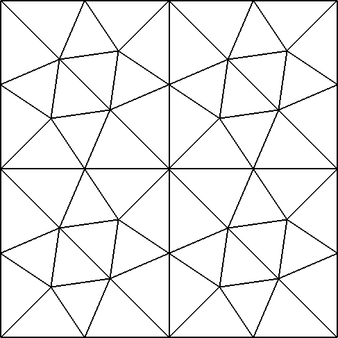
(a) “tri”

(b) “cart”

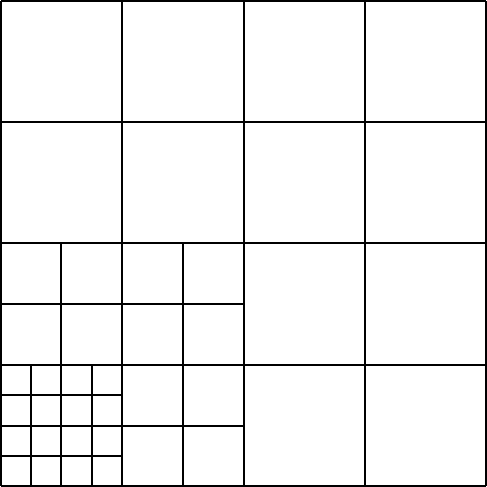
(c) “locref”

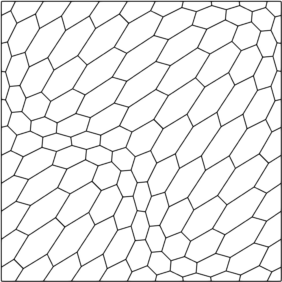
(d) “hexa”

Figure 1: Mesh families used in the numerical tests of Section 6.

$h$ $k$ System size $\|\underline{u}_{h}-\underline{I}_{U,h}u\|_{1,h}$ OCV $\|\nabla_{h}(r_{h}\underline{u}_{h}-u)\|_{L^{2}(\Omega)^{d\times d}}$ OCV $\|u_{h}-I_{U,h}u\|_{L^{2}(\Omega)^{d}}$ OCV $\|r_{h}\underline{u}_{h}-u\|_{L^{2}(\Omega)^{d}}$ OCV $\|p_{h}-I_{P,h}p\|_{L^{2}(\Omega)}$ OCV $\nu=1$ 0.25 0 393 3.222194e-02 – 2.358650e-02 – 3.157105e-03 – 1.079341e-03 – 8.353185e-03 – 0.125 0 1569 1.568367e-02 1.04 1.176665e-02 1.00 8.130095e-04 1.96 3.173216e-04 1.77 3.715999e-03 1.17 0.0625 0 6273 7.890606e-03 0.99 5.860134e-03 1.01 2.087535e-04 1.96 9.097616e-05 1.80 1.359228e-03 1.45 0.03125 0 25089 3.978745e-03 0.99 2.918938e-03 1.01 5.300457e-05 1.98 2.430899e-05 1.90 4.747372e-04 1.52 0.015625 0 100353 1.999853e-03 0.99 1.456954e-03 1.00 1.335882e-05 1.99 6.269384e-06 1.96 1.753818e-04 1.44 0.25 1 637 1.261567e-02 – 4.381984e-03 – 4.005323e-04 – 1.423174e-04 – 2.270947e-03 – 0.125 1 2561 3.012656e-03 2.07 1.239913e-03 1.82 5.094272e-05 2.97 2.011596e-05 2.82 6.069516e-04 1.90 0.0625 1 10273 7.423158e-04 2.02 3.140934e-04 1.98 6.487856e-06 2.97 2.558775e-06 2.97 1.515679e-04 2.00 0.03125 1 41153 1.846133e-04 2.01 7.882465e-05 1.99 8.261358e-07 2.97 3.225663e-07 2.99 3.765641e-05 2.01 0.015625 1 164737 4.606087e-05 2.00 1.974435e-05 2.00 1.046304e-07 2.98 4.050395e-08 2.99 9.359506e-06 2.01 0.25 2 881 4.901561e-03 – 6.467589e-04 – 7.339555e-05 – 1.163225e-05 – 3.628231e-04 – 0.125 2 3553 5.784949e-04 3.08 8.006862e-05 3.01 4.193709e-06 4.13 7.971323e-07 3.87 4.640113e-05 2.97 0.0625 2 14273 6.973436e-05 3.05 9.896615e-06 3.02 2.512826e-07 4.06 5.200708e-08 3.94 5.795639e-06 3.00 0.03125 2 57217 8.605670e-06 3.02 1.246030e-06 2.99 1.554178e-08 4.02 3.388334e-09 3.94 7.286071e-07 2.99 0.015625 2 229121 1.070946e-06 3.01 1.570128e-07 2.99 9.699535e-10 4.00 2.175903e-10 3.96 9.142654e-08 2.99 $\nu=0.001$ 0.25 0 393 3.222194e-02 – 2.358650e-02 – 3.157105e-03 – 1.079341e-03 – 8.353185e-06 – 0.125 0 1569 1.568367e-02 1.04 1.176665e-02 1.00 8.130095e-04 1.96 3.173216e-04 1.77 3.715999e-06 1.17 0.0625 0 6273 7.890606e-03 0.99 5.860134e-03 1.01 2.087535e-04 1.96 9.097616e-05 1.80 1.359228e-06 1.45 0.03125 0 25089 3.978745e-03 0.99 2.918938e-03 1.01 5.300457e-05 1.98 2.430899e-05 1.90 4.747372e-07 1.52 0.015625 0 100353 1.999853e-03 0.99 1.456954e-03 1.00 1.335882e-05 1.99 6.269384e-06 1.96 1.753818e-07 1.44 0.25 1 637 1.261567e-02 – 4.381984e-03 – 4.005323e-04 – 1.423174e-04 – 2.270947e-06 – 0.125 1 2561 3.012656e-03 2.07 1.239913e-03 1.82 5.094272e-05 2.97 2.011596e-05 2.82 6.069516e-07 1.90 0.0625 1 10273 7.423158e-04 2.02 3.140934e-04 1.98 6.487856e-06 2.97 2.558775e-06 2.97 1.515679e-07 2.00 0.03125 1 41153 1.846133e-04 2.01 7.882465e-05 1.99 8.261358e-07 2.97 3.225663e-07 2.99 3.765641e-08 2.01 0.015625 1 164737 4.606087e-05 2.00 1.974435e-05 2.00 1.046304e-07 2.98 4.050395e-08 2.99 9.359506e-09 2.01 0.25 2 881 4.901561e-03 – 6.467589e-04 – 7.339555e-05 – 1.163225e-05 – 3.628231e-07 – 0.125 2 3553 5.784949e-04 3.08 8.006862e-05 3.01 4.193709e-06 4.13 7.971323e-07 3.87 4.640113e-08 2.97 0.0625 2 14273 6.973436e-05 3.05 9.896615e-06 3.02 2.512826e-07 4.06 5.200708e-08 3.94 5.795639e-09 3.00 0.03125 2 57217 8.605670e-06 3.02 1.246030e-06 2.99 1.554178e-08 4.02 3.388334e-09 3.94 7.286071e-10 2.99 0.015625 2 229121 1.070946e-06 3.01 1.570128e-07 2.99 9.699535e-10 4.00 2.175903e-10 3.96 9.142654e-11 2.99 $\nu=1e-06$ 0.25 0 393 3.222194e-02 – 2.358650e-02 – 3.157105e-03 – 1.079341e-03 – 8.353185e-09 – 0.125 0 1569 1.568367e-02 1.04 1.176665e-02 1.00 8.130095e-04 1.96 3.173216e-04 1.77 3.715999e-09 1.17 0.0625 0 6273 7.890606e-03 0.99 5.860134e-03 1.01 2.087535e-04 1.96 9.097616e-05 1.80 1.359228e-09 1.45 0.03125 0 25089 3.978745e-03 0.99 2.918938e-03 1.01 5.300457e-05 1.98 2.430899e-05 1.90 4.747372e-10 1.52 0.015625 0 100353 1.999853e-03 0.99 1.456954e-03 1.00 1.335882e-05 1.99 6.269385e-06 1.96 1.753818e-10 1.44 0.25 1 637 1.261567e-02 – 4.381984e-03 – 4.005323e-04 – 1.423174e-04 – 2.270947e-09 – 0.125 1 2561 3.012656e-03 2.07 1.239913e-03 1.82 5.094272e-05 2.97 2.011596e-05 2.82 6.069516e-10 1.90 0.0625 1 10273 7.423158e-04 2.02 3.140934e-04 1.98 6.487856e-06 2.97 2.558775e-06 2.97 1.515679e-10 2.00 0.03125 1 41153 1.846133e-04 2.01 7.882465e-05 1.99 8.261358e-07 2.97 3.225663e-07 2.99 3.765642e-11 2.01 0.015625 1 164737 4.606087e-05 2.00 1.974435e-05 2.00 1.046304e-07 2.98 4.050395e-08 2.99 9.359491e-12 2.01 0.25 2 881 4.901561e-03 – 6.467589e-04 – 7.339556e-05 – 1.163225e-05 – 3.628230e-10 – 0.125 2 3553 5.784949e-04 3.08 8.006862e-05 3.01 4.193709e-06 4.13 7.971323e-07 3.87 4.640111e-11 2.97 0.0625 2 14273 6.973438e-05 3.05 9.896615e-06 3.02 2.512827e-07 4.06 5.200708e-08 3.94 5.795651e-12 3.00 0.03125 2 57217 8.605698e-06 3.02 1.246029e-06 2.99 1.554182e-08 4.02 3.388331e-09 3.94 7.285984e-13 2.99 0.015625 2 229121 1.072212e-06 3.00 1.570176e-07 2.99 9.707280e-10 4.00 2.176095e-10 3.96 9.160016e-14 2.99 $\nu=1e-09$ 0.25 0 393 3.222197e-02 – 2.358650e-02 – 3.157101e-03 – 1.079343e-03 – 8.353126e-12 – 0.125 0 1569 1.568351e-02 1.04 1.176655e-02 1.00 8.128663e-04 1.96 3.172635e-04 1.77 3.716196e-12 1.17 0.0625 0 6273 7.890564e-03 0.99 5.860114e-03 1.01 2.086862e-04 1.96 9.094945e-05 1.80 1.359335e-12 1.45 0.03125 0 25089 3.978735e-03 0.99 2.918933e-03 1.01 5.297332e-05 1.98 2.429646e-05 1.90 4.747921e-13 1.52 0.015625 0 100353 1.999850e-03 0.99 1.456953e-03 1.00 1.334166e-05 1.99 6.262585e-06 1.96 1.754138e-13 1.44 0.25 1 637 1.261571e-02 – 4.381978e-03 – 4.005307e-04 – 1.423153e-04 – 2.270990e-12 – 0.125 1 2561 3.012621e-03 2.07 1.239912e-03 1.82 5.093999e-05 2.98 2.011354e-05 2.82 6.069569e-13 1.90 0.0625 1 10273 7.422844e-04 2.02 3.140926e-04 1.98 6.486999e-06 2.97 2.558201e-06 2.97 1.515955e-13 2.00 0.03125 1 41153 1.849331e-04 2.00 7.882788e-05 1.99 8.264979e-07 2.97 3.225103e-07 2.99 3.774118e-14 2.01 0.015625 1 164737 4.819223e-05 1.94 1.975600e-05 2.00 1.062163e-07 2.96 4.051995e-08 2.99 9.917517e-15 1.93 0.25 2 881 4.901606e-03 – 6.467540e-04 – 7.339583e-05 – 1.163162e-05 – 3.628306e-13 – 0.125 2 3553 5.784848e-04 3.08 8.006882e-05 3.01 4.193606e-06 4.13 7.971120e-07 3.87 4.645136e-14 2.97 0.0625 2 14273 7.017755e-05 3.04 9.899016e-06 3.02 2.526041e-07 4.05 5.206829e-08 3.94 6.384613e-15 2.86 0.03125 2 57217 1.670814e-05 2.07 1.294704e-06 2.93 2.775679e-08 3.19 3.717234e-09 3.81 3.168766e-15 1.01 0.015625 2 229121 5.230319e-05 -1.65 1.214343e-06 0.09 3.896141e-08 -0.49 1.919767e-09 0.95 5.651455e-15 -0.83

Table 3: Numerical results for the Botti–Massa method of Section 5.2.

$h$ $k$ System size $\|\underline{u}_{h}-\underline{I}_{U,h}u\|_{1,h}$ OCV $\|\nabla_{h}(r_{h}\underline{u}_{h}-u)\|_{L^{2}(\Omega)^{d\times d}}$ OCV $\|u_{h}-I_{U,h}u\|_{L^{2}(\Omega)^{d}}$ OCV $\|r_{h}\underline{u}_{h}-u\|_{L^{2}(\Omega)^{d}}$ OCV $\|p_{h}-I_{P,h}p\|_{L^{2}(\Omega)}$ OCV $\nu=1$ 0.25 0 301 5.091366e-02 – 3.763716e-02 – 5.452321e-03 – 2.192226e-03 – 1.057235e-02 – 0.125 0 1217 2.664248e-02 0.93 1.953002e-02 0.95 1.438660e-03 1.92 6.349527e-04 1.79 5.209898e-03 1.02 0.0625 0 4897 1.371812e-02 0.96 9.874165e-03 0.98 3.749484e-04 1.94 1.811691e-04 1.81 1.987649e-03 1.39 0.03125 0 19649 6.961800e-03 0.98 4.949384e-03 1.00 9.571999e-05 1.97 4.831682e-05 1.91 6.963471e-04 1.51 0.015625 0 78721 3.504377e-03 0.99 2.476364e-03 1.00 2.416339e-05 1.99 1.243355e-05 1.96 2.562386e-04 1.44 0.25 1 545 1.260873e-02 – 5.067568e-03 – 4.695794e-04 – 1.661224e-04 – 2.574142e-03 – 0.125 1 2209 3.495394e-03 1.85 1.437499e-03 1.82 6.391980e-05 2.88 2.394042e-05 2.79 7.023496e-04 1.87 0.0625 1 8897 9.150857e-04 1.93 3.657393e-04 1.97 8.347818e-06 2.94 3.061214e-06 2.97 1.747567e-04 2.01 0.03125 1 35713 2.353234e-04 1.96 9.211973e-05 1.99 1.076894e-06 2.95 3.867520e-07 2.98 4.309645e-05 2.02 0.015625 1 143105 5.983437e-05 1.98 2.312937e-05 1.99 1.373785e-07 2.97 4.860589e-08 2.99 1.063320e-05 2.02 0.25 2 789 1.989339e-03 – 7.215444e-04 – 4.092264e-05 – 1.437024e-05 – 5.024945e-04 – 0.125 2 3201 1.714420e-04 3.54 9.153136e-05 2.98 1.755080e-06 4.54 1.012735e-06 3.83 6.278277e-05 3.00 0.0625 2 12897 1.816462e-05 3.24 1.149733e-05 2.99 9.536951e-08 4.20 6.728081e-08 3.91 7.930655e-06 2.98 0.03125 2 51777 2.172452e-06 3.06 1.459545e-06 2.98 5.795572e-09 4.04 4.417584e-09 3.93 1.011191e-06 2.97 0.015625 2 207489 2.715882e-07 3.00 1.846122e-07 2.98 3.642384e-10 3.99 2.845126e-10 3.96 1.280167e-07 2.98 $\nu=0.001$ 0.25 0 301 5.091366e-02 – 3.763716e-02 – 5.452321e-03 – 2.192226e-03 – 1.057235e-05 – 0.125 0 1217 2.664248e-02 0.93 1.953002e-02 0.95 1.438660e-03 1.92 6.349527e-04 1.79 5.209898e-06 1.02 0.0625 0 4897 1.371812e-02 0.96 9.874165e-03 0.98 3.749484e-04 1.94 1.811691e-04 1.81 1.987649e-06 1.39 0.03125 0 19649 6.961800e-03 0.98 4.949384e-03 1.00 9.571999e-05 1.97 4.831682e-05 1.91 6.963471e-07 1.51 0.015625 0 78721 3.504377e-03 0.99 2.476364e-03 1.00 2.416339e-05 1.99 1.243355e-05 1.96 2.562386e-07 1.44 0.25 1 545 1.260873e-02 – 5.067568e-03 – 4.695794e-04 – 1.661224e-04 – 2.574142e-06 – 0.125 1 2209 3.495394e-03 1.85 1.437499e-03 1.82 6.391980e-05 2.88 2.394042e-05 2.79 7.023496e-07 1.87 0.0625 1 8897 9.150857e-04 1.93 3.657393e-04 1.97 8.347818e-06 2.94 3.061214e-06 2.97 1.747567e-07 2.01 0.03125 1 35713 2.353234e-04 1.96 9.211973e-05 1.99 1.076894e-06 2.95 3.867520e-07 2.98 4.309645e-08 2.02 0.015625 1 143105 5.983437e-05 1.98 2.312937e-05 1.99 1.373785e-07 2.97 4.860589e-08 2.99 1.063320e-08 2.02 0.25 2 789 1.989339e-03 – 7.215444e-04 – 4.092264e-05 – 1.437024e-05 – 5.024945e-07 – 0.125 2 3201 1.714420e-04 3.54 9.153136e-05 2.98 1.755080e-06 4.54 1.012735e-06 3.83 6.278277e-08 3.00 0.0625 2 12897 1.816462e-05 3.24 1.149733e-05 2.99 9.536951e-08 4.20 6.728081e-08 3.91 7.930655e-09 2.98 0.03125 2 51777 2.172452e-06 3.06 1.459545e-06 2.98 5.795572e-09 4.04 4.417584e-09 3.93 1.011191e-09 2.97 0.015625 2 207489 2.715882e-07 3.00 1.846122e-07 2.98 3.642384e-10 3.99 2.845126e-10 3.96 1.280167e-10 2.98 $\nu=1e-06$ 0.25 0 301 5.091366e-02 – 3.763716e-02 – 5.452321e-03 – 2.192226e-03 – 1.057235e-08 – 0.125 0 1217 2.664248e-02 0.93 1.953002e-02 0.95 1.438660e-03 1.92 6.349527e-04 1.79 5.209898e-09 1.02 0.0625 0 4897 1.371812e-02 0.96 9.874165e-03 0.98 3.749484e-04 1.94 1.811691e-04 1.81 1.987649e-09 1.39 0.03125 0 19649 6.961800e-03 0.98 4.949384e-03 1.00 9.571999e-05 1.97 4.831682e-05 1.91 6.963471e-10 1.51 0.015625 0 78721 3.504377e-03 0.99 2.476364e-03 1.00 2.416339e-05 1.99 1.243355e-05 1.96 2.562386e-10 1.44 0.25 1 545 1.260873e-02 – 5.067568e-03 – 4.695794e-04 – 1.661224e-04 – 2.574142e-09 – 0.125 1 2209 3.495394e-03 1.85 1.437499e-03 1.82 6.391980e-05 2.88 2.394042e-05 2.79 7.023496e-10 1.87 0.0625 1 8897 9.150857e-04 1.93 3.657393e-04 1.97 8.347818e-06 2.94 3.061214e-06 2.97 1.747568e-10 2.01 0.03125 1 35713 2.353234e-04 1.96 9.211973e-05 1.99 1.076894e-06 2.95 3.867520e-07 2.98 4.309646e-11 2.02 0.015625 1 143105 5.983437e-05 1.98 2.312937e-05 1.99 1.373785e-07 2.97 4.860590e-08 2.99 1.063319e-11 2.02 0.25 2 789 1.989339e-03 – 7.215444e-04 – 4.092264e-05 – 1.437023e-05 – 5.024945e-10 – 0.125 2 3201 1.714420e-04 3.54 9.153136e-05 2.98 1.755080e-06 4.54 1.012735e-06 3.83 6.278276e-11 3.00 0.0625 2 12897 1.816462e-05 3.24 1.149733e-05 2.99 9.536949e-08 4.20 6.728081e-08 3.91 7.930667e-12 2.98 0.03125 2 51777 2.172451e-06 3.06 1.459544e-06 2.98 5.795567e-09 4.04 4.417579e-09 3.93 1.011182e-12 2.97 0.015625 2 207489 2.717105e-07 3.00 1.846151e-07 2.98 3.643416e-10 3.99 2.845273e-10 3.96 1.281173e-13 2.98 $\nu=1e-09$ 0.25 0 301 5.091363e-02 – 3.763719e-02 – 5.452310e-03 – 2.192225e-03 – 1.057255e-11 – 0.125 0 1217 2.664234e-02 0.93 1.952987e-02 0.95 1.438559e-03 1.92 6.348927e-04 1.79 5.210224e-12 1.02 0.0625 0 4897 1.371811e-02 0.96 9.874163e-03 0.98 3.749366e-04 1.94 1.811630e-04 1.81 1.987694e-12 1.39 0.03125 0 19649 6.961792e-03 0.98 4.949376e-03 1.00 9.569553e-05 1.97 4.830410e-05 1.91 6.963895e-13 1.51 0.015625 0 78721 3.504375e-03 0.99 2.476363e-03 1.00 2.415342e-05 1.99 1.242844e-05 1.96 2.562572e-13 1.44 0.25 1 545 1.260861e-02 – 5.067566e-03 – 4.695673e-04 – 1.661151e-04 – 2.574172e-12 – 0.125 1 2209 3.495056e-03 1.85 1.437494e-03 1.82 6.390885e-05 2.88 2.393561e-05 2.79 7.023477e-13 1.87 0.0625 1 8897 9.149967e-04 1.93 3.657387e-04 1.97 8.346386e-06 2.94 3.060646e-06 2.97 1.747808e-13 2.01 0.03125 1 35713 2.353216e-04 1.96 9.212023e-05 1.99 1.076851e-06 2.95 3.867169e-07 2.98 4.316424e-14 2.02 0.015625 1 143105 5.989604e-05 1.97 2.313613e-05 1.99 1.374942e-07 2.97 4.863242e-08 2.99 1.107310e-14 1.96 0.25 2 789 1.989319e-03 – 7.215433e-04 – 4.092234e-05 – 1.437001e-05 – 5.025068e-13 – 0.125 2 3201 1.714564e-04 3.54 9.153210e-05 2.98 1.755206e-06 4.54 1.012769e-06 3.83 6.282424e-14 3.00 0.0625 2 12897 1.826850e-05 3.23 1.149849e-05 2.99 9.575826e-08 4.20 6.730105e-08 3.91 8.367764e-15 2.91 0.03125 2 51777 3.348559e-06 2.45 1.494559e-06 2.94 8.286685e-09 3.53 4.796850e-09 3.81 3.193360e-15 1.39 0.015625 2 207489 8.084852e-06 -1.27 9.689466e-07 0.63 8.450114e-09 -0.03 2.358977e-09 1.02 5.357670e-15 -0.75

Table 4: Numerical results for the new method with Raviart–Thomas–Nédélec velocities at elements of Section 5.4.

$h$ $k$ System size $\|\underline{u}_{h}-\underline{I}_{U,h}u\|_{1,h}$ OCV $\|\nabla_{h}(r_{h}\underline{u}_{h}-u)\|_{L^{2}(\Omega)^{d\times d}}$ OCV $\|u_{h}-I_{U,h}u\|_{L^{2}(\Omega)^{d}}$ OCV $\|r_{h}\underline{u}_{h}-u\|_{L^{2}(\Omega)^{d}}$ OCV $\|p_{h}-I_{P,h}p\|_{L^{2}(\Omega)}$ OCV “tri” mesh family 0.25 0 301 2.871509e-01 – 1.388025e-01 – 2.593695e-02 – 1.600589e-02 – 1.181657e-01 – 0.125 0 1217 1.777113e-01 0.69 8.032856e-02 0.79 8.742641e-03 1.57 6.711338e-03 1.25 7.136302e-02 0.73 0.0625 0 4897 1.056728e-01 0.75 4.066457e-02 0.98 2.754628e-03 1.67 2.345353e-03 1.52 3.546204e-02 1.01 0.03125 0 19649 5.919433e-02 0.84 1.909566e-02 1.09 7.961755e-04 1.79 7.104760e-04 1.72 1.499777e-02 1.24 0.015625 0 78721 3.155741e-02 0.91 8.815891e-03 1.12 2.154894e-04 1.89 1.964997e-04 1.85 5.693412e-03 1.40 0.25 1 545 1.094570e-01 – 1.442178e-02 – 3.566780e-03 – 5.455960e-04 – 9.971271e-03 – 0.125 1 2209 2.864697e-02 1.93 4.029509e-03 1.84 4.708069e-04 2.92 7.396471e-05 2.88 2.444760e-03 2.03 0.0625 1 8897 7.259557e-03 1.98 1.048116e-03 1.94 5.981108e-05 2.98 9.481457e-06 2.96 5.908448e-04 2.05 0.03125 1 35713 1.824671e-03 1.99 2.671313e-04 1.97 7.525256e-06 2.99 1.202422e-06 2.98 1.452048e-04 2.02 0.015625 1 143105 4.572920e-04 2.00 6.745664e-05 1.99 9.435208e-07 3.00 1.516119e-07 2.99 3.603847e-05 2.01 0.25 2 789 2.229905e-02 – 1.419633e-03 – 4.267495e-04 – 3.575930e-05 – 1.104445e-03 – 0.125 2 3201 2.913007e-03 2.94 2.057320e-04 2.79 2.782726e-05 3.94 2.784274e-06 3.68 1.603266e-04 2.78 0.0625 2 12897 3.697032e-04 2.98 2.803240e-05 2.88 1.766127e-06 3.98 1.983784e-07 3.81 2.182177e-05 2.88 0.03125 2 51777 4.652907e-05 2.99 3.679046e-06 2.93 1.112016e-07 3.99 1.332765e-08 3.90 2.855088e-06 2.93 0.015625 2 207489 5.835491e-06 3.00 4.719275e-07 2.96 6.976227e-09 3.99 8.650121e-10 3.95 3.653625e-07 2.97 “cart” mesh family 0.141421 0 681 7.431549e-02 – 5.434746e-02 – 8.757928e-03 – 6.594299e-03 – 6.380900e-02 – 0.0707107 0 2761 3.107123e-02 1.26 2.721935e-02 1.00 2.655586e-03 1.72 2.306187e-03 1.52 3.273492e-02 0.96 0.0353553 0 11121 1.241095e-02 1.32 1.190420e-02 1.19 7.555894e-04 1.81 7.039030e-04 1.71 1.413110e-02 1.21 0.0176777 0 44641 4.881669e-03 1.35 4.782175e-03 1.32 2.034841e-04 1.89 1.960254e-04 1.84 5.418242e-03 1.38 0.141421 1 1261 2.231652e-02 – 2.071433e-03 – 5.267229e-04 – 3.493709e-05 – 7.189385e-04 – 0.0707107 1 5121 5.649050e-03 1.98 4.834399e-04 2.10 6.658733e-05 2.98 3.655879e-06 3.26 9.922670e-05 2.86 0.0353553 1 20641 1.418751e-03 1.99 1.153138e-04 2.07 8.350360e-06 3.00 3.970154e-07 3.20 1.301183e-05 2.93 0.0176777 1 82881 3.553536e-04 2.00 2.813487e-05 2.04 1.044885e-06 3.00 4.589223e-08 3.11 1.674172e-06 2.96 0.141421 2 1841 2.306263e-03 – 2.086652e-04 – 2.840043e-05 – 2.186706e-06 – 1.069296e-04 – 0.0707107 2 7481 2.916838e-04 2.98 2.723758e-05 2.94 1.793080e-06 3.99 1.453602e-07 3.91 1.532567e-05 2.80 0.0353553 2 30161 3.672161e-05 2.99 3.453053e-06 2.98 1.127570e-07 3.99 9.301390e-09 3.97 2.018631e-06 2.92 0.0176777 2 121121 4.610043e-06 2.99 4.335188e-07 2.99 7.073963e-09 3.99 5.863440e-10 3.99 2.574813e-07 2.97 “locref” mesh family 0.176777 0 1121 9.662929e-02 – 6.562072e-02 – 1.260023e-02 – 8.866492e-03 – 7.575972e-02 – 0.0883883 0 4481 4.099609e-02 1.24 3.436386e-02 0.93 3.906079e-03 1.69 3.286328e-03 1.43 4.145393e-02 0.87 0.0441942 0 17921 1.652976e-02 1.31 1.560495e-02 1.14 1.135878e-03 1.78 1.043778e-03 1.65 1.880963e-02 1.14 0.0220971 0 71681 6.483533e-03 1.35 6.378802e-03 1.29 3.108131e-04 1.87 2.979813e-04 1.81 7.448419e-03 1.34 0.176777 1 2081 3.419560e-02 – 2.922194e-03 – 1.009461e-03 – 6.113120e-05 – 1.309813e-03 – 0.0883883 1 8321 8.705068e-03 1.97 6.775391e-04 2.11 1.285386e-04 2.97 6.530443e-06 3.23 1.873541e-04 2.81 0.0441942 1 33281 2.190150e-03 1.99 1.594929e-04 2.09 1.615289e-05 2.99 6.990477e-07 3.22 2.489209e-05 2.91 0.0220971 1 133121 5.489024e-04 2.00 3.859099e-05 2.05 2.022588e-06 3.00 7.936535e-08 3.14 3.227847e-06 2.95 0.176777 2 3041 4.385363e-03 – 3.551913e-04 – 6.724034e-05 – 4.645085e-06 – 1.904914e-04 – 0.0883883 2 12161 5.582283e-04 2.97 4.762003e-05 2.90 4.278387e-06 3.97 3.194758e-07 3.86 2.847426e-05 2.74 0.0441942 2 48641 7.038299e-05 2.99 6.108618e-06 2.96 2.695583e-07 3.99 2.082572e-08 3.94 3.835956e-06 2.89 0.0220971 2 194561 8.841014e-06 2.99 7.707985e-07 2.99 1.692408e-08 3.99 1.324258e-09 3.98 4.942612e-07 2.96 “hexa” mesh family 0.241412 0 1162 5.770683e-02 – 6.001934e-02 – 8.695028e-03 – 7.650827e-03 – 7.183858e-02 – 0.129713 0 4322 2.732537e-02 1.20 3.083595e-02 1.07 3.271674e-03 1.57 3.088796e-03 1.46 3.427624e-02 1.19 0.0657364 0 16642 1.135351e-02 1.29 1.347297e-02 1.22 1.012115e-03 1.73 9.847495e-04 1.68 1.426008e-02 1.29 0.0329799 0 65282 4.499879e-03 1.34 5.454410e-03 1.31 2.820949e-04 1.85 2.784537e-04 1.83 5.489740e-03 1.38 0.241412 1 2202 1.590592e-02 – 4.250048e-03 – 4.983831e-04 – 2.051919e-04 – 3.726391e-03 – 0.129713 1 8202 4.682540e-03 1.97 1.069133e-03 2.22 7.943574e-05 2.96 2.543882e-05 3.36 7.854022e-04 2.51 0.0657364 1 31602 1.239505e-03 1.96 2.457061e-04 2.16 1.069243e-05 2.95 2.458947e-06 3.44 1.487627e-04 2.45 0.0329799 1 124002 3.171237e-04 1.98 5.656809e-05 2.13 1.373283e-06 2.98 2.383934e-07 3.38 2.744157e-05 2.45 0.241412 2 3242 2.485494e-03 – 4.271783e-04 – 4.614337e-05 – 9.897321e-06 – 2.615419e-04 – 0.129713 2 12082 4.180162e-04 2.87 7.454427e-05 2.81 4.305935e-06 3.82 9.444987e-07 3.78 4.017522e-05 3.02 0.0657364 2 46562 5.918798e-05 2.88 1.066472e-05 2.86 3.168190e-07 3.84 7.066557e-08 3.81 5.338156e-06 2.97 0.0329799 2 182722 7.815297e-06 2.94 1.411474e-06 2.93 2.122297e-08 3.92 4.763964e-09 3.91 6.820794e-07 2.98

Table 5: Numerical results for the polytopal method of Section 5.5.

References

• [1] J. Aghili, S. Boyaval and D.. Di Pietro “Hybridization of mixed high-order methods on general meshes and application to the Stokes equations” In Comput. Meth. Appl. Math. 15.2, 2015, pp. 111–134 DOI: 10.1515/cmam-2015-0004
• [2] B. Ayuso de Dios, K. Lipnikov and G. Manzini “The nonconforming virtual element method” In ESAIM: Math. Model Numer. Anal. 50.3, 2016, pp. 879–904 DOI: 10.1051/m2an/2015090
• [3] S. Baier-Reino and G.. Wells “Analysis of Pressure-Robust Embedded-Hybridized Discontinuous Galerkin Methods for the Stokes Problem Under Minimal Regularity” In J. Sci. Comput. 92.51, 2022 DOI: 10.1007/s10915-022-01889-6
• [4] Lourenço Beirão da Veiga, Franco Dassi, Daniele A. Di Pietro and Jérôme Droniou “Arbitrary-order pressure-robust DDR and VEM methods for the Stokes problem on polyhedral meshes” In Comput. Meth. Appl. Mech. Engrg. 397.115061, 2022 DOI: 10.1016/j.camwa.2022.08.041
• [5] L. Belenki, L.. Berselli, L. Diening and M. Růžička “On the finite element approximation of $p$-Stokes systems” In SIAM J. Numer. Anal. 50.2, 2012, pp. 373–397 DOI: 10.1137/10080436X
• [6] D. Boffi, F. Brezzi and M. Fortin “Mixed finite element methods and applications” 44, Springer Series in Computational Mathematics Heidelberg: Springer, 2013, pp. xiv+685 DOI: 10.1007/978-3-642-36519-5
• [7] L. Botti and F.. Massa “HHO methods for the incompressible Navier-Stokes and the incompressible Euler equations” In J. Sci. Comput. 92.28, 2022 DOI: 10.1007/s10915-022-01864-1
• [8] Lorenzo Botti, Daniele A. Di Pietro and Jérôme Droniou “A Hybrid High-Order discretisation of the Brinkman problem robust in the Darcy and Stokes limits” In Comput. Methods Appl. Mech. Engrg. 341, 2018, pp. 278–310 DOI: 10.1016/j.cma.2018.07.004
• [9] M. Botti, D. Castanon Quiroz, D.. Di Pietro and A. Harnist “A Hybrid High-Order method for creeping flows of non-Newtonian fluids” In ESAIM: Math. Model Numer. Anal. 55.5, 2021, pp. 2045–2073 DOI: 10.1051/m2an/2021051
• [10] S.. Brenner “Forty years of the Crouzeix-Raviart element” In Numer. Methods PDEs 31.2, 2014, pp. 367–396 DOI: 10.1002/num.21892
• [11] F. Brezzi, J.. Douglas, M. Fortin and L.. Marini “Efficient rectangular mixed finite elements in two and three space variables” In ESAIM: Math. Model Numer. Anal. 21.4, 1987, pp. 581–604 DOI: 10.1051/m2an/1987210405811
• [12] D. Castanon Quiroz and D.. Di Pietro “A Hybrid High-Order method for the incompressible Navier–Stokes problem robust for large irrotational body forces” In Comput. Math. Appl. 79.8, 2020, pp. 2655–2677 DOI: 10.1016/j.camwa.2019.12.005
• [13] D. Castanon Quiroz and D.. Di Pietro “A pressure-robust HHO method for the solution of the incompressible Navier–Stokes equations on general meshes” In IMA J. Numer. Anal. 44.1, 2024, pp. 397–434 DOI: 10.1093/imanum/drad007
• [14] A. Cesmelioglu, B. Cockburn and W. Qiu “Analysis of a hybridizable discontinuous Galerkin method for the steady-state incompressible Navier-Stokes equations” In Math. Comp. 86.306, 2017, pp. 1643–1670 DOI: 10.1090/mcom/3195
• [15] B. Cockburn, D.. Di Pietro and A. Ern “Bridging the Hybrid High-Order and Hybridizable Discontinuous Galerkin methods” In ESAIM: Math. Model. Numer. Anal. 50.3, 2016, pp. 635–650 DOI: 10.1051/m2an/2015051
• [16] B. Cockburn and J. Gopalakrishnan “The derivation of hybridizable discontinuous Galerkin methods for Stokes flow” In SIAM J. Numer. Anal. 47.2, 2009, pp. 1092–1125 DOI: 10.1137/080726653
• [17] B. Cockburn, J. Gopalakrishnan, N.. Nguyen, J. Peraire and F.-J. Sayas “Analysis of HDG methods for Stokes flow” In Math. Comp. 80.274, 2011, pp. 723–760 DOI: 10.1090/S0025-5718-2010-02410-X
• [18] B. Cockburn, G. Kanschat and D. Schötzau “A note on Discontinuous Galerkin divergence-free solutions of the Navier–Stokes equations” In J. Sci. Comput. 31.190, 2007, pp. 61–73 DOI: 10.1007/s10915-006-9107-7
• [19] M. Crouzeix and P.-A. Raviart “Conforming and nonconforming finite element methods for solving the stationary Stokes equations” In RAIRO Modél. Math. Anal. Num. 7.3, 1973, pp. 33–75
• [20] D.. Di Pietro and J. Droniou “A polytopal method for the Brinkman problem robust in all regimes” In Comput. Meth. Appl. Mech. Engrg. 409.115981, 2023 DOI: 10.1016/j.cma.2023.115981
• [21] D.. Di Pietro and J. Droniou “A third Strang lemma for schemes in fully discrete formulation” In Calcolo 55.40, 2018 DOI: 10.1007/s10092-018-0282-3
• [22] D.. Di Pietro and J. Droniou “The Hybrid High-Order method for polytopal meshes”, Modeling, Simulation and Application 19 Springer International Publishing, 2020 DOI: 10.1007/978-3-030-37203-3
• [23] D.. Di Pietro, J. Droniou and J.. Qian “A pressure-robust Discrete de Rham scheme for the Navier–Stokes equations” In Comput. Meth. Appl. Mech. Engrg. 421.116765, 2024 DOI: 10.1016/j.cma.2024.116765
• [24] D.. Di Pietro and A. Ern “Mathematical aspects of discontinuous Galerkin methods” 69, Mathématiques & Applications (Berlin) [Mathematics & Applications] Springer, Heidelberg, 2012, pp. xviii+384 DOI: 10.1007/978-3-642-22980-0
• [25] D.. Di Pietro, A. Ern, A. Linke and F. Schieweck “A discontinuous skeletal method for the viscosity-dependent Stokes problem” In Comput. Meth. Appl. Mech. Engrg. 306, 2016, pp. 175–195 DOI: 10.1016/j.cma.2016.03.033
• [26] D. Frerichs and C. Merdon “Divergence-preserving reconstructions on polygons and a really pressure-robust virtual element method for the Stokes problem” In IMA J. Numer. Anal. 42.1, 2022, pp. 597–619 DOI: 10.1093/imanum/draa073
• [27] V. John, A. Linke, C. Merdon, M. Neilan and L.. Rebholz “On the divergence constraint in mixed finite element methods for incompressible flows” In SIAM Rev. 59.3, 2017, pp. 492–544
• [28] Keegan L.. Kirk and Sander Rhebergen “Analysis of a Pressure-Robust Hybridized Discontinuous Galerkin Method for the Stationary Navier–Stokes Equations” In J. Sci. Comput. 81.2, 2019, pp. 881–897 DOI: 10.1007/s10915-019-01040-y
• [29] C. Kreuzer, R. Verfürth and P. Zanotti “Quasi-Optimal and Pressure Robust Discretizations of the Stokes Equations by Moment- and Divergence-Preserving Operators” In Comp. Meth. Appl. Math. 21.2, 2021, pp. 423–443 DOI: 10.1515/cmam-2020-0023
• [30] C. Kreuzer and P. Zanotti “Quasi-optimal and pressure-robust discretizations of the Stokes equations by new augmented Lagrangian formulations” In IMA J. Numer. Anal. 40.4, 2020, pp. 2553–2583 DOI: 10.1093/imanum/drz044
• [31] P.. Lederer, A. Linke, C. Merdon and J. Schöberl “Divergence-free reconstruction operators for pressure-robust Stokes discretization s with continuous pressure finite elements” In SIAM J. Numer. Anal. 55.3, 2017, pp. 1291–1314 DOI: 10.1137/16M10899
• [32] C. Lehrenfeld and J. Schöberl “High order exactly divergence-free Hybrid Discontinuous Galerkin Methods for unsteady incompressible flows” In Comput. Methods Appl. Mech. Engrg. 307, 2016, pp. 339–361 DOI: 10.1016/j.cma.2016.04.025
• [33] A. Linke and C. Merdon “Pressure-robustness and discrete Helmholtz projectors in mixed finite element methods for the incompressible Navier-Stokes equations” In Comput. Methods Appl. Mech. Engrg. 311, 2016, pp. 304–326 DOI: 10.1016/j.cma.2016.08.018
• [34] Alexander Linke “On the role of the Helmholtz decomposition in mixed methods for incompressible flows and a new variational crime” In Comput. Methods Appl. Mech. Engrg. 268, 2014, pp. 782–800 DOI: 10.1016/j.cma.2013.10.011
• [35] Sander Rhebergen and Garth N. Wells “A hybridizable discontinuous Galerkin method for the Navier-Stokes equations with pointwise divergence-free velocity field” In J. Sci. Comput. 76.3, 2018, pp. 1484–1501 DOI: 10.1007/s10915-018-0671-4
• [36] J. Wang and X. Ye “New Finite Element Methods in Computational Fluid Dynamics by $H(div)$ Elements” In SIAM Journal on Numerical Analysis 45.3, 2007, pp. 1269–1286 DOI: 10.1137/060649227
• [37] J. Zhao, B. Zhang, S. Mao and S. Chen “The nonconforming virtual element method for the Darcy–Stokes problem” In Comput. Methods Appl. Mech. Engrg. 370.113251, 2020 DOI: 10.1016/j.cma.2020.113251