Cosmology from String T-duality and zero-point length

Abstract

Inspired by String T-duality and taking into account the zero-point length correction, $l_{0}$, to the gravitational potential, we construct modified Friedmann equations by applying the first law of thermodynamics on the apparent horizon of the Friedmann-Robertson-Walker (FRW) Universe. The cosmological viability of this extended scenario is investigated by studying influences on the evolution of the early Universe and performing the cosmographic analysis. Furthermore, we explore the inflationary paradigm under the slow-roll condition. By testing the model against observational data, the zero-point length is constrained around the Planck scale, in compliance with the original assumption from String T-duality. We also study the growth of density perturbations in the linear regime. It is shown that the zero-point length stands out as an alternative characterization for the broken-power-law spectrum, which provides a better fitting for the experimental measurements comparing to the simple power-law potential. Finally, we focus on implications for the primordial gravitational waves (PGWs) spectrum. Should the zero-point length be running over energy scales, as is the case for all parameters and coupling constants in quantum gravity under renormalization group considerations, deviations from General Relativity (GR) might be potentially tested through upcoming PGW observatories.

I Introduction

Nowadays, it is a general belief that laws of gravity may be regarded as a manifestation of laws of thermodynamics for the large scale spacetime systems. This idea has been well established in the past three decades, where it has been confirmed that the gravitational field equations can be constructed from the first law of thermodynamics on the boundary of spacetime Jac ; Pad1 ; Pad2 . This approach is also reversible, namely one can start from gravitational field equations governing dynamics of the system in the bulk and show that it can be rewritten in the form of the first law of thermodynamics on the boundary of the system Pad3 . The deep connection between thermodynamics and gravity has been explored in different setups. In particular, in the context of FRW cosmology, it has been shown that the Friedmann equations describing the evolution of the Universe can be rewritten as the first law of thermodynamics on the apparent horizon and vice versa CaiKim ; Cai2 ; wang1 ; SheyWC ; SheyWC2 ; SheyCQ .

Although GR has successfully passed a number of experimental and observational tests, it still suffers from some problems such as curvature singularity at the center of black holes or initial singularity in the standard cosmology. Removing these singularities, using the first principles and fundamental theories such as string theory and quantum gravity, is one of the main challenges of modern theoretical physics. To relax singularity in the black hole solutions, regular black holes were proposed by combining the non-linear electrodynamics with Einstein-Hilbert Lagrangian RegBH1 ; RegBH2 . An attempt towards constructing singularity free black holes was performed by averaging noncommutative coordinates on suitable coherent states in string theory Nico1 ; Nico2 ; Nico3 . It was argued that the effects of noncommutative is equivalent to a nonlocal deformation of the Einstein-Hilbert action Nico4 ; Mod .

Another approach to deal with nonsingular black holes comes from the concept of T-duality in string theory. It was argued that the momentum space propagator induced by the path integral duality, for a particle with mass $m_{0}$, is given by Padm ; Sma ; Spa ; Fon

$$G(p)=-\frac{l_{0}}{\sqrt{p^{2}+m_{0}^{2}}}K_{1}\left(l_{0}\sqrt{p^{2}+m_{0}^{2}}\right),$$ (1)

where $p^{2}=(\hbar k)^{2}$ is now the squared momentum, $l_{0}$ represents the zero-point length of spacetime and $K_{1}(x)$ is a modified Bessel function of the second kind. For the massless particles the above propagator can be written as ($\hbar=1$) td1

$$G(k)=-\frac{l_{0}}{\sqrt{k^{2}}}K_{1}\left(l_{0}\sqrt{k^{2}}\right).$$ (2)

In the limiting case where $(l_{0}k^{2})\rightarrow 0$, one find $G(k)=-k^{-2}$ for the massless propagator.

The static Newtonian potential corresponding to $G(k)$ at distance $r$ is obtained as td1

$$V(r)=-\frac{M}{\sqrt{r^{2}+l_{0}^{2}}},$$ (3)

where $M$ is the mass of the source of the potential. It has been shown that this finite potential changes the metric around an electrically neutral black hole and leads to a regular spacetime at $r=0$ td1 . Besides, it modifies the Hawking temperature, the entropy associated with the horizon, and hence thermodynamics of black holes td1 .

Following the entropic force scenario proposed by Verlinde Ver , the effects of zero-point length on the Newton’s law of gravity were explored in KS . Nevertheless, since cosmology can explore physics at higher energy scales, it seems natural that the implications of the zero-point length could be more likely tested in this context. On the cosmological scales, Eq. (3) along with Verlinde’s conjecture lead to correction terms to the Newtonian cosmology, while in the relativistic regime they give rise to modified Friedmann equations in a FRW background KS . This procedure also leads to a modified expression for the entropy, due to the zero-point length, associated with the horizon, which is useful in studying thermodynamics of the Universe. In passing, we mention that the hypothesis of modified horizon entropy is widespread across many extended theories of gravity, see for instance ME1 ; ME2 ; ME3 ; ME4 ; ME6 ; ME7 ; ME8 and references therein.

Using thermodynamics-gravity conjecture and applying the first law of thermodynamics on the apparent horizon, in this work we derive the modified cosmological field equations in the presence of zero-point length from string T-duality. Research in this direction has been active in the last three decades Q0 ; Q1 ; Q2 ; Q3 , focusing primarily on the development of a minimal-length cosmology in the framework of the generalized uncertainty principle Lit1 ; Lit2 ; Lit3 ; Lit4 ; Lit5 ; Lit6 ; Lit7 ; Lit8 ; Lit9 ; Lit10 . Compared to the previous efforts, our analysis provides an advancement in understanding the semiclassical regime of quantum cosmology. Indeed, on the one hand we offer an alternative perspective by embedding a minimal length from a novel theoretical standpoint. On the other hand, we explore phenomenological consequences of the obtained modified field equations on a wide range of energy scales, including implications for the dynamics of the Universe in the radiation and matter dominated eras, the early inflation, the growth of perturbations and gravitational waves. To the best of our knowledge, such a dedicated analysis has not yet been considered in literature. On top of that, we extract a constraint on the zero-point length. The result aligns with the original assumption that this cutoff scale is identifiable with the Planck length Padm , as well as with the recent estimate of the zero-point length in the context of quantum corrected black holes td1 .

The work is structured as follows. In the next section we develop a modified cosmological scenario based on the zero-point length and study its implications for the evolution of the Universe. Section III is devoted to analyze of inflation, while in Sec. IV we focus on the growth of perturbations and structure formation. Effects on the spectrum of primordial gravitational waves are explored in Sec. V. The discussion of closing remarks and perspectives is reserved for Sec. VI. Unless otherwise stated, we shall use Planck units $\hslash=c=G=k_{B}=1$.

II Modified Friedman Equations through zero-point length

According to T-duality the zero-point length affects the gravitational potential td1 . Thus, the gravitational potential of a spherical mass distribution $M$ at distance $r=R$ is modified as td2 ; td3

$$\phi(r)=-\frac{M}{\sqrt{r^{2}+l_{0}^{2}}}|_{r=R},$$ (4)

where $l_{0}$ is the zero-point length and its value is expected to be of Planck length td1 . Thus the Newton’s law of gravity for a mass point $m$ get modified as

$$\vec{F}=-m\vec{\nabla}\phi(r)|_{r=R}=-\frac{Mm}{R^{2}}\left[1+\frac{l_{0}^{2}}{R^{2}}\right]^{-3/2}\hat{r}.$$ (5)

Using the entropic force scenario, this leads to correction to the entropy associated with the horizon as KS

$$1+\left(\frac{1}{2\pi R}\right)\frac{d{s}}{dR}=\left(1+\frac{l_{0}^{2}}{R^{2}}\right)^{-3/2}$$ (6)

where $s$ is the correction term to the total entropy of the horizon,

$$S_{h}=\frac{A}{4}+s(A).$$ (7)

and $A=4\pi R^{2}$ is the area of the horizon enveloped the volume $V=4\pi R^{3}/3$. Combining Eqs. (6) and (7), we arrive at

$$dS_{h}=2\pi R\left(1+\frac{l_{0}^{2}}{R^{2}}\right)^{-3/2}dR\,.$$ (8)

Before moving onto the cosmological analysis, it is noteworthy that deviations from the area-law scaling are very common in quantum gravity, e.g. in string theory Log1 , loop quantum gravity Log2 , AdS/CFT correspondence Carlip , generalized uncertainty principle Log3 , etc. Additionally, entropic corrections appear from entanglement entropy calculations in four spacetime dimensions at UV scale UV1 ; UV2 . Therefore, despite the specific String T-duality framework we are considering here, our next arguments are expected to have more general validity in the context of quantum gravity.

Let us assume our Universe is described by the line element

$$ds^{2}={h}_{\mu\nu}dx^{\mu}dx^{\nu}+R^{2}(d\theta^{2}+\sin^{2}\theta d\phi^{2}),$$ (9)

where $R=a(t)r$, $x^{0}=t,x^{1}=r$, and $h_{\mu\nu}$=diag $(-1,a^{2}/(1-kr^{2}))$ stands for the two dimensional metric. $k=-1,0,1$ represents the curvature of the Universe and $a$ the (time-dependent) scale factor. The apparent horizon is the suitable boundary of the Universe from thermodynamic viewpoint, which has radius SheyLog

$$R=\frac{1}{\sqrt{H^{2}+k/a^{2}}}.$$ (10)

The associated temperature with the horizon is given by Cai2 ; Sheyem

$$T_{h}=-\frac{1}{2\pi R}\left(1-\frac{\dot{R}}{2HR}\right),$$ (11)

where the overdot denotes derivative with respect to the cosmic time $t$. For an adiabatic expansion, one may assume $\dot{R}\ll 2HR$ in the infinitesimal interval $dt$, which physically implies that the apparent horizon radius is kept nearly fixed CaiKim .

The total energy momentum tensor is assumed in the form of the perfect fluid

$$T_{\mu\nu}=(\rho+p)u_{\mu}u_{\nu}+pg_{\mu\nu},$$ (12)

where $\rho$ and $p$ are the energy density and pressure, respectively. The conservation of energy for the metric leads to

$$\dot{\rho}+3H(\rho+p)=0,$$ (13)

where $H=\dot{a}/a$ is the Hubble parameter. The work density due to the volume change of the Universe is Hay2

$$W=-\frac{1}{2}T^{\mu\nu}h_{\mu\nu}=\frac{1}{2}(\rho-p).$$ (14)

Taking differential form of the total energy $E=\rho(4\pi R^{3}/3)$ and using the conservation equation (13), we find

$$dE=4\pi\tilde{r}_{A}^{2}\rho d\tilde{r}_{A}-4\pi H\tilde{r}_{A}^{3}(\rho+p)dt.$$ (15)

Inserting Eqs. (8), (11), (14), (15) in the first law of thermodynamics on the apparent horizon, $dE=T_{h}dS_{h}+WdV$, and using the definition (11) for the temperature, after some calculations, one gets

$$4\pi HR^{3}(\rho+p)dt=\left(1+\frac{l_{0}^{2}}{R^{2}}\right)^{-3/2}dR.$$ (16)

Using the continuity equation (13), we arrive at

$$-\frac{2}{R^{3}}\left(1+\frac{l_{0}^{2}}{R^{2}}\right)^{-3/2}dR=\frac{8\pi}{3}d\rho.$$ (17)

After integrating, we have

$$-\frac{2}{l_{0}^{2}}\left(1+\frac{l_{0}^{2}}{R^{2}}\right)^{-1/2}+C=\frac{8\pi}{3}\rho,$$ (18)

where $C$ is the constant of integration. Since ${l_{0}^{2}}/{R^{2}}$ is expected to be small, we can expand the LHS of the above equations. We find

$$-\frac{2}{l_{0}^{2}}\left[1-\frac{l_{0}^{2}}{2R^{2}}+\frac{3}{8}\frac{l_{0}^{4}}{R^{4}}+\mathcal{O}\left(\frac{l_{0}}{R}\right)^{6}\right]+C=\frac{8\pi}{3}\rho.$$ (19)

Clearly, in the limiting case where $l_{0}^{2}\rightarrow 0$, we must restore the standard Friedmann equation. Thus, we set

$$C\equiv\frac{2}{l_{0}^{2}}-\frac{\Lambda}{3},$$ (20)

where $\Lambda$ is the cosmological constant. The final form of the modified Friedmann equation is obtained as

$$H^{2}+\frac{k}{a^{2}}-\alpha\left(H^{2}+\frac{k}{a^{2}}\right)^{2}+\mathcal{O}(\alpha^{2})=\frac{8\pi}{3}\rho+\frac{\Lambda}{3},$$ (21)

where $\alpha=3l_{0}^{2}/4$, and we have used relation (10). In a flat Universe ($k=0$), the above Friedmann equation reads

$$H^{2}-\alpha H^{4}=\frac{8\pi}{3}\rho+\frac{\Lambda}{3}.$$ (22)

As we can see, the use of the modified entropy (7) results to a modified Friedmann equation, with an extra term comparing to GR. In passing, we notice that such correction could be re-interpreted as an effective dark energy sector by recasting Eq. (22) as

$$H^{2}=\frac{8\pi}{3}\left(\rho+\rho_{DE}\right),$$ (23)

where

$$\rho_{DE}=\frac{3}{8\pi}\left(\frac{\Lambda}{3}+\alpha H^{4}\right).$$ (24)

Similarly, the modified second Friedmann equation can be derived by differentiating Eq. (23) with respect to $t$ and using Eq. (13). After some algebra, we obtain

$$\dot{H}=-4\pi\left[\rho+p+\rho_{DE}+p_{DE}\right],$$ (25)

where we have defined the pressure of the effective dark energy sector as

$$p_{DE}=-\frac{1}{8\pi}\left[\Lambda+\alpha H^{2}\left(4\dot{H}+3H^{2}\right)\right].$$ (26)

Hence, the effective equation of state becomes

$$w_{DE}=\frac{p_{DE}}{\rho_{DE}}=-1-\frac{4\alpha H^{2}\dot{H}}{3\alpha H^{4}+\Lambda}=-1-\frac{4\alpha H^{2}\dot{H}}{\Lambda}+\mathcal{O}(\alpha^{2}).$$ (27)

We would like to notice, however, that in the forthcoming analysis we do not conceptualize the zero-point length correction as an effective dark energy contribute. Instead, we adhere to the original interpretation of T-duality and consider the additional term as due to a modified description of gravity.

As expected, in the case $\alpha=0$, the modified Friedmann equations (23) and (25) reduce to the $\Lambda\textrm{CDM}$ paradigm

$$H^{2} = \frac{8\pi}{3}\rho+\frac{\Lambda}{3}\,,$$ (28)

$$\dot{H} = -4\pi\left(\rho+p\right).$$ (29)

II.1 Cosmological solutions

Now we study the cosmological implications of the zero-point length scenario. We shall consider the interesting case where the perfect fluid includes dust matter ($p_{m}\approx 0$) and radiation. From the continuity equation, these components components evolve according to

$$\rho_{m} = \rho_{m,0}a^{-3}\,,$$ (30)

$$\rho_{r} = \rho_{r,0}a^{-4}\,,$$ (31)

where the subscript “0” denotes the values at present time and we set $a_{0}=1$.

Dividing both side of Eq. (22) by $H_{0}^{2}$, we find

$$-\beta\left(\frac{H}{H_{0}}\right)^{4}+\left(\frac{H}{H_{0}}\right)^{2}-\Omega_{m,0}a^{-3}-\Omega_{r,0}a^{-4}-\Omega_{\Lambda,0}=0\,,$$ (32)

where

$$\beta\equiv\alpha H_{0}^{2}=\frac{3}{4}l_{0}^{2}H_{0}^{2}\ll 1\,,$$ (33)

and we have introduced the dimensionless density parameters

$$\Omega_{i} = \frac{8\pi}{3H^{2}}\rho_{i},\quad(i=m,r)\,,$$ (34)

$$\Omega_{\Lambda} = \frac{\Lambda}{3H^{2}}\,.$$ (35)

To convert $\beta$ in terms of the dimensional zero-point length, it proves convenient to restore for a while the gravitational constant $G=\ell_{p}^{2}=6.7\times 10^{-39}\,\mathrm{GeV}^{-2}$, where $\ell_{p}$ is the Planck length. For $H_{0}\simeq 10^{-42}\,\mathrm{GeV}$, we find $l_{0}\simeq 1.4\times 10^{61}\sqrt{\beta}\ell_{p}$. Coming back to our original units, we have

$$l_{0}\simeq 1.4\times 10^{61}\sqrt{\beta}\,.$$ (36)

Therefore, $l_{0}\sim\mathcal{O}(1)$ corresponds to $\beta\sim\mathcal{O}(10^{-122})$.

Now, solving Eq. (32), we are led to

$$\left(\frac{H}{H_{0}}\right)^{2}=\frac{1}{2\beta}\left\{1-\sqrt{1-4\beta\left[\Omega_{m,0}a^{-3}+\Omega_{r,0}a^{-4}+\Omega_{\Lambda,0}\right]}\right\}.$$ (37)

Since $\beta$ is expected to be small, we can expand the RHS to the linear order. The result is

$$\frac{H^{2}}{H_{0}^{2}}=\left(\Omega_{m,0}a^{-3}+\Omega_{r,0}a^{-4}+\Omega_{\Lambda,0}\right)$$ (38)

$$\times\left[1+\beta\left(\Omega_{m,0}a^{-3}+\Omega_{r,0}a^{-4}+\Omega_{\Lambda,0}\right)\right]+\mathcal{O}(\beta^{2})\,.$$

If we define, as usual, the redshift parameter as

$$\frac{1}{a}=1+z\,,$$ (39)

we can rewrite Eq. (38) as

$$\frac{H^{2}(z)}{H_{0}^{2}}=\left[\Omega_{m,0}\left(1+z\right)^{3}+\Omega_{r,0}\left(1+z\right)^{4}+\Omega_{\Lambda,0}\right]$$ (40)

$$\times\left\{1+\beta\left[\Omega_{m,0}\left(1+z\right)^{3}+\Omega_{r,0}\left(1+z\right)^{4}+\Omega_{\Lambda,0}\right]\right\}+\mathcal{O}(\beta^{2})\,.$$

The value of $\Omega_{\Lambda,0}$ can be set by imposing the flatness condition $H(0)/H_{0}=1$, which gives

$$\Omega_{\Lambda,0}=1-\Omega_{m,0}-\Omega_{r,0}-\beta+\mathcal{O}(\beta^{2})\,.$$ (41)

A relevant quantity in understanding the dynamics governing the Universe’s evolution is the deceleration parameter

$$q=-1-\frac{\dot{H}}{H^{2}}=-1+\left(1+z\right)\frac{\partial_{z}H}{H}\,.$$ (42)

For $q>0$, the expansion of the Universe is decelerating, which implies that the gravitational pull of matter dominates over any other influences, causing the expansion to slow down over time. On the other hand, $q<0$ signifies an accelerating Universe. The discovery of the accelerated expansion, supported by observations of distant type Ia Supernovae meas1 ; meas2 and the CMB SDSS:2005xqv , has led to the acceptance of the existence of some exotic component that exerts negative pressure and counteracts the gravitational attraction of matter.

Implications of the zero-point length on the acceleration of the Universe can be studied by plugging Eq. (37) into (42). We get

$$q = \frac{\Omega_{m,0}\left(1+z\right)^{3}+2\Omega_{r,0}\left(1+z\right)^{4}-2\Omega_{\Lambda,0}}{2\left[\Omega_{m,0}\left(1+z\right)^{3}+\Omega_{r,0}\left(1+z\right)^{4}+\Omega_{\Lambda,0}\right]}$$

$$+\,\frac{\beta}{2}\left[3\Omega_{m,0}\left(1+z\right)^{3}+4\Omega_{r,0}\left(1+z\right)^{4}\right]+\mathcal{O}(\beta^{2})\,.$$

At present time, this reduces to

$$q_{0}=-1+\frac{3}{2}\Omega_{m,0}+2\Omega_{r,0}+\beta\left(3\Omega_{m,0}+4\Omega_{r,0}\right)+\mathcal{O}(\beta^{2})\,,$$ (44)

where we have used the condition (41). Notice that, in the limiting case where $\beta=0$, we obtain $q_{0}=-1+\frac{3}{2}\Omega_{m,0}+2\Omega_{r,0}$, which correctly reproduces the $\Lambda$CDM expression.

It might be interesting to constrain $\beta$ using the observational value $q_{0}=-0.56^{+0.04(0.09)}_{-0.04(0.08)}$ CapozDag . Substitution into Eq. (44) with $\Omega_{m,0}\simeq 0.3$ and $\Omega_{r,0}\simeq 5\times 10^{-5}$ yields $\beta<\mathcal{O}(10^{-1})$. Additionally, for such range of values of $\beta$, the transition from deceleration to acceleration phase would occur at redshift $z_{t}\in[0.48,0,75]$, which aligns with the estimate $z_{t}=0.789^{+0.186}_{-0.165}$ derived from the combined CC+BAO+SNeIa dataset (see also Naik:2023ykt ). It should be noted, however, that the above constraint on $\beta$ provides a very weak condition. This could somehow be expected, since it is inferred from measurements of cosmic parameters at present time. A more stringent bound will be derived below through the study of inflation.

II.1.1 Matter dominated era

Let us now investigate the impact of the zero-point length on the dynamics of the scale factor. For the matter dominated era, neglecting the effects of radiation and cosmological constants, Eq. (38) can be approximated as

$$\frac{H^{2}}{H_{0}^{2}}=\Omega_{m,0}a^{-3}\left(1+\beta\Omega_{m,0}a^{-3}\right)+\mathcal{O}(\beta^{2}).$$ (45)

The explicit form of the scale factor as a function of time is obtained by integrating the above relation. We find

$$a(t)=\left[\frac{9}{4}\Omega_{m,0}\left(H_{0}^{2}t^{2}-\frac{4}{9}\beta\right)\right]^{\frac{1}{3}}\,.$$ (46)

where we have set the integration constant equal to zero. This is indeed the case if we assume $a\rightarrow 0$ as $t\rightarrow 0$.

The plot in Fig. 1 shows that the modified scale factor lies below the standard curve for $t$ small enough and vanishes for $H_{0}t=2\sqrt{\beta}/3>0$. Below this threshold, Eq. (46) apparently takes complex values. This is, however, a “border” regime, since we are extrapolating our model to scales comparable or lower than the zero-point length, where the approximation (19) fails. Clearly, such phenomenon indicates a breakdown of the conventional Cosmology approaching $l_{0}$ and the need for a comprehensive quantum gravity framework. On the other hand, $a(t)$ approaches the standard behavior as the Universe evolves for sufficiently large $t$, since the zero-point length corrections become increasingly negligible. In the limiting case where $\beta=0$, one recovers $a(t)\sim t^{2/3}$, which is the well-known solution in standard Cosmology for the matter dominated Universe.

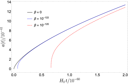
Figure 1: Plot of $a(t)$ versus $H_{0}t$ for the matter dominated era and various values of $\beta$. We set $\Omega_{m,0}\simeq 0.3$.

II.1.2 Radiation dominated era

For the radiation dominated era, the Friedmann equation (38) can be rewritten as

$$\frac{H^{2}}{H_{0}^{2}}=\Omega_{r,0}a^{-4}\left(1+\beta\Omega_{r,0}a^{-4}\right)+\mathcal{O}(\beta^{2}).$$ (47)

In this case the modified scale factor is obtained as

$$a(t)=\left[4\Omega_{r,0}\left(H_{0}^{2}t^{2}-\frac{\beta}{4}\right)\right]^{1/4}\,.$$ (48)

where again we have set the integration constant equal to zero. The curves in Fig. 2 display the same qualitative behavior as discussed in the previous case, both for small and large $t$. When $\beta=0$, one recovers $a(t)\sim t^{1/2}$, which is the expected result in standard Cosmology for the radiation dominated epoch.

For later convenience, we notice that the $a$-dependence in Eq. (47) can be converted to a temperature-dependence through the condition $Ta(t)=T_{0}$, where $T_{0}\simeq 3\,\mathrm{K}$ is the average temperature of the observable Universe at present time. The latter holds true for any $\beta$, as it can be checked by using the relation $\rho\sim T^{4}$ along with Eqs. (31) and (48). In terms of redshift, we can equivalently write

$$\frac{T}{T_{0}}=z+1\,.$$ (49)

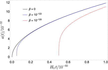
Figure 2: Plot of $a(t)$ versus $H_{0}t$ for the matter dominated era and various values of $\beta$. We set $\Omega_{r,0}\simeq 5\times 10^{-5}$.

II.2 Cosmographic Analysis

The depiction of the Universe, as established by the cosmological principle, is referred to as cosmography WeinbergBook . Cosmography deals with the study of geometric properties, embedding dimensionless higher derivative terms of the scale factor Visser . For the FRW Universe, the latter can be expanded as

$$a(t)=1+\sum_{n=1}^{\infty}\frac{1}{n!}\frac{d^{n}a}{dt^{n}}\left(t-t_{0}\right)^{n}\,.$$ (50)

The coefficients of this Taylor expansion are usually referred to as cosmographic parameters. It is easy to check that the first two parameters are related with the Hubble rate and deceleration parameter, respectively. On the other hand, the third derivative of the scale factor with respect to cosmic time gives the jerk parameter Jerk1 ; Jerk2

$$j=\frac{1}{aH^{3}}\frac{d^{3}a}{dt^{3}}=q\left(2q+1\right)+\left(1+z\right)\frac{dq}{dz}\,,$$ (51)

which is useful in understanding the acceleration of the Universe and, in particular, the departure of a cosmological model from the $\Lambda$CDM.

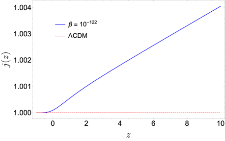
Figure 3: Plot of $j(z)$ versus $z$ (blue solid curve). The red dashed line sets the $\Lambda$CDM value $j=1$. We set $\Omega_{m,0}\simeq 0.3$ and $\Omega_{r,0}\simeq 5\times 10^{-5}$.

The evolution of $j$ as a function of redshift is plotted in Fig. 3 (blue solid curve) in comparison with the $\Lambda$CDM prediction $j=1$ (red dashed line). The analytical computation is easily performed by plugging Eq. (II.1) into (51). As expected, our model mostly deviates from the $\Lambda$CDM at higher redshift, while the standard description is recovered approaching the present time. This observation prompts the anticipation of an alternative description of early Universe in the presence of zero-point length. Furthermore, we find $j>0$, which is consistent with an accelerated expansion.

Although the first three cosmographic parameters are sufficient to determine the overall kinematics of the Universe CapozCosm , it is sometimes convenient to consider extra terms in the expansion (50). For example, the snap parameter $s$ is a dimensionless quantity that describes the fourth derivative of the scale factor of the Universe with respect to cosmic time. It provides information about the rate of change of acceleration in the expansion of the Universe, thus characterizing the dynamics of cosmic acceleration. Following Pan:2017ent , we have

$$s=\frac{1}{aH^{4}}\frac{d^{4}a}{dt^{4}}=-j\left(2+3q\right)-\left(1+z\right)\frac{dj}{dz}\,.$$ (52)

Clearly, for the $\Lambda$CDM model $s=-(2+3q)$ since $j=1$. Thus, the departure of $ds/dq$ from $-3$ quantifies the deviation of the evolution of the Universe from the $\Lambda$CDM dynamics.

By using Eqs. (II.1) and (51), we infer the evolution of $s$ in the presence of zero-point length (see Fig. 4). For such small values of $\beta$, deviations from the $\Lambda$CDM model are hardly appreciable in this case even at high redshifts. Observing the behavior of $s$, it is evident that it assumes negative values in the early Universe, transitioning to positive values as the evolution progresses. At present time $s_{0}\simeq-0.2$, consistently with the observational estimate of the deceleration parameter $q_{0}\simeq-0.6$.

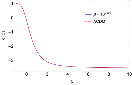
Figure 4: Plot of $s(z)$ versus $z$ (blue solid curve). The red dashed curve gives the $\Lambda$CDM prediction. We set $\Omega_{m,0}\simeq 0.3$ and $\Omega_{r,0}\simeq 5\times 10^{-5}$.

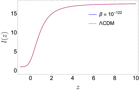
Figure 5: Plot of $l(z)$ versus $z$ (blue solid curve). The red dashed curve gives the $\Lambda$CDM prediction. We set $\Omega_{m,0}\simeq 0.3$ and $\Omega_{r,0}\simeq 5\times 10^{-5}$.

Let us finally consider the lerk parameter, which is given by the fifth derivative of the scale factor as Pan:2017ent

$$l=\frac{1}{aH^{5}}\frac{d^{5}a}{dt^{5}}=-s\left(3+4q\right)-\left(1+z\right)\frac{ds}{dz}\,.$$ (53)

The evolution of $l$ is plotted in Fig. 5, which displays that the lerk parameter exclusively maintains positive values. Similar to the jerk parameter $j$, both the snap parameter s and the lerk parameter $l$ tend to unity during the later stages of the Universe’s evolution. This trend emphasizes the consistent dynamics exhibited by these parameters in our model.

III Slow-roll inflation in zero-point length Cosmology

Since the zero-point length is expected to primarily influence the evolution of the early Universe, in this Section we investigate its implications for inflation. This phase is usually described in terms of a hypothetical scalar field $\phi$ - the inflaton - which is thought to have been the driving force behind the inflationary expansion. The dynamics of the inflaton field is governed by the (spatially homogenous) potential $V(\phi)$.

Under the canonical scalar field assumption, the model lagrangian takes the usual form $\mathcal{L}=X-V(\phi)$, where $X=-\frac{1}{2}h^{\mu\nu}\partial_{\mu}\phi\hskip 0.56905pt\partial_{\nu}\phi$ is the kinetic term. The energy density and pressure for the inflation are

$$\rho_{\phi} = \frac{\dot{\phi}^{2}}{2}+V(\phi)\,,$$ (54)

$$p_{\phi} = \frac{\dot{\phi}^{2}}{2}-V(\phi)\,.$$ (55)

The continuity equation (13) implies the dynamics

$$\ddot{\phi}+3H\dot{\phi}+\partial_{\phi}V(\phi)=0\,,$$ (56)

where $\partial_{\phi}V\equiv\frac{dV}{d\phi}$.

The successful models of inflation are typically characterized by a very flat potential along which the inflaton rolls down towards a minimum. If the evolution of the field occurs so slowly that the kinetic energy is negligible compared to the potential term, then the inflaton exhibits a cosmological constant-like behavior, leading to an exponential expansion of the Universe. During this phase, which is referred to as slow-roll inflation, matter and radiation components are diluted away rapidly, allowing us to neglect all sources of energy density other than the inflaton.

Mathematically speaking, the slow-roll approximation is expressed by the conditions Luciano:2023roh ; Keskin ; OdSR

$$\ddot{\phi} \ll H\dot{\phi}\,,$$ (57)

$$\frac{\dot{\phi}^{2}}{2} \ll V(\phi)\,.$$ (58)

The second relation effectively states that $V(\phi)$ is nearly constant, since the inflaton changes very slowly in time. This implies that the Hubble rate remains approximately constant. Therefore, it proves useful to introduce the dimensionless parameter

$$\epsilon\equiv-\frac{\dot{H}}{H^{2}}\,,$$ (59)

where it is understood that $\epsilon\ll 1$. Additionally, to keep track of the relative change of $\epsilon$ per Hubble time, we define a second slow-roll parameter as

$$\eta\equiv\frac{\dot{\epsilon}}{H\epsilon}\,.$$ (60)

For a sufficiently long inflation, it is likewise needed $\eta\ll 1$.

The total amount of expansion that occurred during inflation is quantified by the number of e-folds efolds

$$\mathcal{N}=\int Hdt=\int\frac{H}{\dot{\phi}}d\phi\,,$$ (61)

from the horizon crossing $\phi_{c}$ to the end of inflation defined by $\epsilon(\phi_{f})=1$. For typical inflationary models, a sensible working hypothesis is $\mathcal{N}$ larger than $\sim 50-60$ Liddlebis , which weakly depends on the inflation scale and the thermal history after inflation. However, an extremely long duration of inflation is not excluded, and appears even necessary in certain scenarios. For example, the stochastic axion framework SAM ; SAM2 , the relaxation scenario Relax and a quintessence model Quint require $\log_{10}\mathcal{N}\sim\mathcal{O}(10)$, depending on model parameters. Recently, a simple single-field model has been proposed in the context of stochastic inflation with an average $e$-folds $\langle\mathcal{N}\rangle\sim{10^{10}}^{10}$ StocInf . In the following, we shall consider more traditional and experimentally favored scenarios involving $\mathcal{O}(10^{2})\lesssim\mathcal{N}\lesssim\mathcal{O}(10^{3})$.

According to the inflationary paradigm, the rapid growth of the Universe caused fluctuations of the scalar field to be stretched to large scales and, upon crossing the horizon, to freeze in. In the Fourier space, such fluctuations are characterized by a power spectrum with spectral index Liddle

$$n_{s}-1=2\eta-6\epsilon\,,$$ (62)

There is another kind of density perturbations, the tensor modes, which are fluctuations in the fabric of spacetime. Similarly to the scalar modes, their spectrum is expected to follow a power-law behavior (see Sec. V for more details). The ratio of the tensor to scalar spectra is given by

$$r=16\epsilon\,.$$ (63)

The parameters (62), (63) play a crucial role, as for the possibility to constrain or rule out inflationary models by comparison with observations. In particular, the latest Planck Public Release 4, BICEP/Keck Array 2018, Planck CMB lensing and BAO data set the experimental bounds $r<0.037$ rconst and $n_{s}\simeq 0.97$ SpecCons1 .

To study how the zero-point length affects the above parameters, we now consider the modified Friedmann equation (22), where we neglect for simplicity the cosmological constant. Using Eq. (54) for the inflaton energy density along with the first slow-roll condition (57), we obtain

$$H(\phi)\simeq\sqrt{\frac{8\pi V}{3}}\left(1+\frac{4\pi\beta}{3H_{0}^{2}}V\right)+\mathcal{O}(\beta^{2})\,,$$ (64)

where the $\phi$-dependence of $V$ has been omitted in the RHS.

On the other hand, by differentiating Eq. (22) with respect to $t$ and using the conditions (54), (55), we find

$$\dot{H}\simeq-4\pi\left(1+\frac{16\pi\beta}{3H_{0}^{2}}V\right)\dot{\phi}^{2}+\mathcal{O}(\beta^{2})\,.$$ (65)

Notice that the time derivative $\dot{\phi}$ can be expressed in terms of $\phi$ through Eq. (56), which in the slow-roll approximation simplifies to

$$\dot{\phi} \simeq -\frac{1}{3H}\partial_{\phi}V$$

$$= \left(-\frac{1}{2\sqrt{6\pi}}+\sqrt{\frac{2\pi}{27}}\frac{\beta}{H_{0}^{2}}V\right)\frac{\partial_{\phi}V}{\sqrt{V}}\,+\,\mathcal{O}(\beta^{2})\,.$$

III.1 Power-law potential

The latter equation indicates that the dynamics of $\phi$ is ruled by the potential $V(\phi)$. It should be noted that two different approaches are typically considered in studying inflation. The dynamically motivated approach involves reconstructing $V$ by requiring the Universe to evolve following a specific dynamics, which is set by a fixed time-dependence of the Hubble rate. From this perspective, inflationary models are classified according to the corresponding Universe evolution. As an example, in DMA the scale factor is set to $a(t)=t^{m}$ for a suitable choice of the power term $m$. Nevertheless, the disadvantage is that the predicted scalar-to-tensor ratio exceeds the constraint set by the BICEP and Planck data. Moreover, the slow-roll parameters turn out to be constant. On the other hand, the potential motivated method involves setting the inflaton potential first and then solving the ensuing Friedmann equations. Such an approach finds wide application in extended theories gravity Liddle ; Keskin ; Luciano:2023roh ; NojiOd ; DiValentino:2016ziq ; Adhikari:2020xcg , where deviations of the dynamics of the early Universe from GR are admitted. Inflationary models are in this case categorized based on the form of the potential, which is fixed a priori.

In order to discuss a concrete model of inflation, in the following we consider the potential motivated approach. Specifically, we assume the power-law form

$$V=V_{0}\phi^{n}\,,$$ (67)

where the amplitude $V_{0}$ and the power term $n$ are both positive constants. Following Liddle ; Luciano:2023roh , $V_{0}$ is set to unity. Although its actual value may vary in a wide range Matarrese , this assumption is justified by the fact that the magnitude of $V_{0}$ is expected not to alter the power-law function during inflation. Furthermore, experimental evidence favors inflationary models with $n\sim\mathcal{O}\left(10^{-1}\div 1\right)$, while $n\geq 2$ tends to be ruled out in the minimal coupling scenario. We shall here consider $n=1$.

With the ansatz (67), the dimensionless parameter (59) is found to be

$$\epsilon(\phi)\simeq\frac{1}{16\pi\phi^{2}}+\mathcal{O}(\beta^{2})\,,$$ (68)

which also allows us to derive the inflaton at the end of inflation as

$$\epsilon(\phi_{f})=1\,\,\Longrightarrow\,\,\phi_{f}\simeq\frac{1}{4\sqrt{\pi}}+\mathcal{O}(\beta^{2})\,.$$ (69)

The spectral index $n_{s}$ and the tensor-to-scalar ratio $r$ are typically evaluated at the horizon crossing, where the fluctuations of the inflaton freeze and remain nearly constant Liddle ; Keskin ; Luciano:2023roh ; LucSheLamb . From Eq. (61), the inflaton at the horizon crossing is obtained as

$$\phi_{c}\simeq\frac{1}{4}\sqrt{\frac{f(\mathcal{N})}{\pi}}+\frac{\beta}{18H_{0}^{2}}\left[\frac{1-\sqrt{f^{3}(\mathcal{N})}}{\sqrt{f(\mathcal{N})}}\right]+\mathcal{O}(\beta^{2})\,,$$ (70)

where we have used the shorthand notation

$$f(\mathcal{N})\equiv 1+4\mathcal{N}\,.$$ (71)

Therefore, the slow-roll parameters (62), (63) become

$$r_{\beta} = 16\epsilon(\phi_{c})$$ (72)

$$\simeq \frac{16}{f(\mathcal{N})}+\frac{64\sqrt{\pi}\beta}{9H_{0}^{2}}\,\frac{\sqrt{f^{3}(\mathcal{N})}-1}{f^{2}(\mathcal{N})}+\mathcal{O}(\beta^{2})\,,$$

$$n_{s}{{}_{\beta}} = 1+2\eta(\phi_{c})-6\epsilon(\phi_{c})$$ (73)

$$\simeq 1+\frac{2}{f(\mathcal{N})}-\frac{8\sqrt{\pi}\beta}{9H_{0}^{2}}\,\frac{5\sqrt{f^{3}(\mathcal{N})}+1}{f^{2}(\mathcal{N})}+\mathcal{O}(\beta^{2})\,.$$

In order to constrain the parameter $\beta$ (or, equivalently, the zero-point length $l_{0}$), let us compare the above expressions with experimental bounds on $n_{s}$ and $r$ (see below Eq. (63)). Assuming the expected-inflation duration $\mathcal{N}\sim\mathcal{O}(10^{3})$, it can be inferred from Fig. 6 that

$$r_{\beta}<0.037\Longrightarrow\l_{0}\lesssim\mathcal{O}(1)\,,$$ (74)

corresponding to $\beta\lesssim\mathcal{O}(10^{-122})$. This turns into the more stringent condition $l_{0}\lesssim\mathcal{O}(10^{-1})$ $(\beta\lesssim\mathcal{O}(10^{-124}))$ for a total number of $e$-folds $\mathcal{N}\sim\mathcal{O}(10^{2})$. Direct substitution into Eq. (73) shows that these bounds are consistent with the observational measurement $n_{s}\simeq 0.97$ too.

Interestingly enough, the above constraints align with the original assumption $l_{0}\lesssim 1$ of the zero-point length from quantum fluctuations of the background spacetime Padm and the recent result td1 in quantum corrected black holes from String T-Duality.

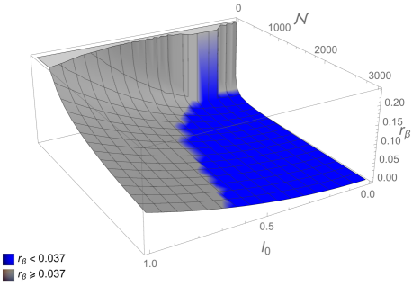
Figure 6: 3D Plot of $r_{\beta}$ versus $\mathcal{N}$ and $l_{0}$. The grey region is excluded by observational constraints rconst .

IV Structure formation

A key challenge in modern Cosmology lies in comprehending the origin and dynamics of perturbation growth during the early Universe, as these fluctuations eventually give rise to the formation of the observed large-scale structures. It is widely accepted that these structures emerge from the amplification of tiny initial density fluctuations through gravitational instability during cosmic evolution. These fluctuations gradually grow until they become sufficiently robust to break away from the background expansion and collapse into gravitationally-bound systems (see Mukhanov:1990me and Malik:2008im for a recent review).

An effective framework for investigating the growth of matter perturbations and structure formation in the linear regime is the Top-Hat Spherical Collapse (SC) model Abramo:2007iu . This approach considers a uniform and spherically symmetric perturbation in an expanding background, describing the growth of perturbations within a spherical region using the Friedmann equations of gravity Planelles:2014zaa . Employing this model, in the following we study the impact of the zero-point length Cosmology on the growth of cosmic perturbations and the power spectrum of scalar fluctuations at the early stages of the Universe.

IV.1 Growth of perturbations in linear regime

As a first step, by using the relation

$$\frac{\ddot{a}}{a}=\dot{H}+H^{2}\,,$$ (75)

let us recast the second modified Friedmann equation as

$$\frac{\ddot{a}}{a}=-\frac{4\pi}{3}\rho\left(1+\frac{32\pi\beta}{3H_{0}^{2}}\rho\right)\,.$$ (76)

To apply the Top-Hat SC model, we focus on a spherical region of radius $a_{p}$ and with a homogenous density $\rho_{c}$. Assume that, at time $t$, $\rho_{c}(t)=\rho(t)+\delta\rho$, where $\delta\rho$ is the density fluctuation. The conservation equation in such simplified spherical region is given by Abramo:2007iu

$$\dot{\rho}_{c}+3h\rho_{c}=0\,,$$ (77)

where $h=\dot{a}_{p}/a_{p}$ denotes the local expansion rate inside the spherical region. The second Friedmann equation applied to this region reads

$$\frac{\ddot{a}_{p}}{a_{p}}=-\frac{4\pi}{3}\rho_{c}\left(1+\frac{32\pi\beta}{3H_{0}^{2}}\rho_{c}\right)\,.$$ (78)

It is now useful to define the density contrast of the fluid by the relation

$$\delta\equiv\frac{\rho_{c}}{\rho}-1=\frac{\delta\rho}{\rho}\,.$$ (79)

Since the fluctuation $\delta\rho$ is expected to be smaller than $\rho$, we can assume $\delta\ll 1$ (linear regime). This is a reasonable approximation, as the initial stages of the gravitational collapse are well described by the linear regime for all but the very smallest sales Abramo:2007iu .

Differentiating Eq. (79) with respect to $t$, we find

$$\dot{\delta}=3\left(1+\delta\right)\left(H-h\right),$$ (80)

where we have used the continuity equation. Further differentiation gives

$$\ddot{\delta}=3\left(1+\delta\right)(\dot{H}-\dot{h})+\frac{\dot{\delta}^{2}}{1+\delta}\,.$$ (81)

Equation (81) governs the dynamics of matter perturbations in the Top-Hat SC model. It can be further manipulated by noting that

$$\dot{H}-\dot{h}=h^{2}-H^{2}+\frac{4\pi\rho}{3}\left(1+\frac{64\pi\beta}{3H_{0}^{2}}\rho\right)\delta+\mathcal{O}(\delta^{2})\,,$$ (82)

where we have neglected higher order terms in $\delta$. After some algebra, substitution into Eq. (81) gives

$$\ddot{\delta}+2H\dot{\delta}-{4\pi\rho}\left(1+\frac{64\pi\beta}{3H_{0}^{2}}\rho\right)\delta+\mathcal{O}(\delta^{2})=0\,.$$ (83)

Changing the time variable to the sale factor $a$, we have

$$\dot{\delta} = aH\delta^{\prime}\,,$$ (84)

$$\ddot{\delta} = a^{2}H^{2}\delta^{\prime\prime}+aH\left(H+aH^{\prime}\right)\delta^{\prime}\,,$$ (85)

where the prime denotes derivative with respect to $a$. Upon substituting into Eq. (83), we obtain

$$\delta^{\prime\prime}+\delta^{\prime}\left(\frac{3}{2a}-\frac{4\pi\beta}{H_{0}^{2}}\frac{\rho}{a}\right)-\delta\left(\frac{3}{2a^{2}}+\frac{28\pi\beta}{H_{0}^{2}}\frac{\rho}{a^{2}}\right)+\mathcal{O}(\delta^{2})=0.$$ (86)

It is easy to check that the standard dynamics is recovered for $\beta\rightarrow 0$ Abramo:2007iu .

Equation (86) has been solved numerically. The solution is plotted in Fig. 7 for various values of $\beta$ consistent with Eq. (74). As expected, effects of the zero-point length mainly manifest as $z$ increases, with the matter density contrast growing more slowly than the standard behavior (black solid curve) in the very early Universe. Therefore, unlike the classical framework, where small-scale fluctuations evolve unhindered, such fluctuations are smoothed out due to the quantum gravity corrections associated with the zero-point length. This smoothing effect limits the growth of fluctuations, leading to a slower increase in the density contrast. A similar suppression has been discussed in Galaxies , assuming a running gravitational constant. Other studies appear in Oth1 ; Oth2 ; Oth3 in the context of full quantum and/or extended gravity.

It should be noted that the above conclusions provide preliminary, but still insightful results toward understanding the effects of zero-point length on the evolution of the density contrast and structure formation. Indeed, for $l_{0}$ around the Planck length, deviations from the classical model could become appreciable at very high redshift, where the linear regime may break down and higher order corrections should be taken into account. A more refined analysis going beyond the linear regime is reserved for the future.

Before moving on, it is interesting to observe that the evolution of matter overdensity $\delta$ is closely related to the $\sigma_{8}$ tension, which quantifies the gravitational matter clustering from the amplitude of the linearly evolved power spectrum at the scale of $8h^{-1}\,\mathrm{Mpc}$. This tension arises from the fact that the Cosmic Microwave Background (CMB) estimation Planck:2018vyg differs from the SDSS/BOSS direct measurements eBOSS:2018cab ; BOSS:2016wmc . The later growth of $\delta$ in Fig. 7 for non-vanishing $\beta$ indicates a less efficient clustering of matter over the time in the presence of a minimal length, which provides a possible mechanism to alleviate the $\sigma_{8}$ tension Heis . A similar outcome in the framework of modified gravity has been found in sig8 using a Tsallis-like deformation of the Bekenstein-Hawking entropy.

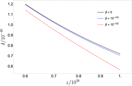
Figure 7: Log-linear plot of $\delta$ versus $z$, for various values of $\beta$. We set the same initial conditions as in Abramo:2007iu .

IV.2 Power spectrum

We now look into the primordial power spectrum for scalar perturbations, which provides an indirect probe of inflation or other structure-formation mechanisms. The simplest inflationary models predict almost purely adiabatic primordial perturbations with a nearly scale-invariant power spectrum given by Har ; Zel

$$P_{\zeta}(k)=A_{S}\left(\frac{k}{k_{*}}\right)^{n_{s}-1}\,,$$ (87)

where $A_{s}\simeq 10^{-9}$ is the power amplitude and $k_{*}$ a characteristic pivot scale.

The form (87) is the statistically preferred by Planck, since it yields a good fit to data with a remarkably small number of parameters. However, it does not provide the best observational fit. Improvements can be obtained by allowing for a deviation from the simple power spectrum, either considering a running spectral index or different functional forms deBlas . This is mainly due to the possibility of suppressing the primordial power spectrum at large scales.

A paradigmatic modification considered by the Planck Collaboration consists in a broken-power-law (bpl) spectrum of the form deBlas

$$P^{bpl}_{\zeta}\propto\left(\frac{k}{k_{*}}\right)^{n_{s}^{bpl}-1+\delta}\,,$$ (88)

for $k$ below a certain cutoff scale. The best fit is obtained for $\delta=1.14$ deBlas .

Interestingly enough, the zero-point length model naturally fits the profile (88). To check this, let us recast Eq. (73) as

$$n_{s}{{}_{\beta}}=n_{s}+g_{\beta}\,,$$ (89)

where $n_{s}$ is the usual spectral index in standard Cosmology ($\beta=0$) and

$$g_{\beta}\equiv-\frac{8\sqrt{\pi}\beta}{9H_{0}^{2}}\,\frac{5\sqrt{f^{3}(\mathcal{N})}+1}{f^{2}(\mathcal{N})}+\mathcal{O}(\beta^{2})$$ (90)

is the zero-point length correction. The latter term has the same role as the $\delta$-shift in the bpl spectrum (88). Said another way, the correction (88) is reproduced in the zero-point length Cosmology while still maintaining the simple power spectrum (87). Indeed, upon replacing the modified spectral index (89), the exponent of Eq. (87) becomes

$$n_{s}-1\,\,\longrightarrow\,\,n_{s}{{}_{\beta}}-g_{\beta}-1\,.$$ (91)

The RHS fits Eq. (88), provided that

$$n_{s}{{}_{\beta}}-g_{\beta}-1=n_{s}^{bpl}-1+\delta\,.$$ (92)

Setting $n_{s}{{}_{\beta}}$ and $n_{s}^{bpl}$ equal to the experimental value SpecCons1 and using Eq. (33), we find

$$l_{0}=\frac{f(\mathcal{N})}{\pi^{1/4}}\sqrt{\frac{3\delta}{2+10f^{3/2}(\mathcal{N})}}\,,$$ (93)

which, for $\mathcal{O}(10^{2})\lesssim N\lesssim\mathcal{O}(10^{3})$ and $\delta=1.14$, gives $l_{0}\sim\mathcal{O}(1)$, in compliance with Eq. (74).

Therefore, zero-point length Cosmology stands out as an alternative characterization for the bpl spectrum, which is still consistent with latest observations.

V Primordial Gravitational Waves

The first ever detection of gravitational waves (GWs) by the LIGO LIGOScientific:2014pky and VIRGO VIRGO:2014yos collaborations has opened up fresh avenues for investigating the Universe. From a theoretical perspective, GWs originate from three main sources categorized based on their generation mechanisms: astrophysical, cosmological and inflationary sources. Astrophysical GWs are notoriously influenced by the mass of the emitting object, with massive compact objects like black holes expected to produce strong GWs. For the minimum mass $M_{\odot}$, for instance, the maximal frequency would be around $10\,\mathrm{kHz}$. On the other hand, various cosmological phenomena in the early Universe, such as first-order phase transitions at $10^{-2}\,\mathrm{GeV}$ or just below the Grand Unified Theory scale, can produce GWs with frequency around $10^{-5}\,\mathrm{Hz}$ or roughly lower than the $\mathrm{GHz}$ range, respectively. Finally, primordial GWs generated during inflation span frequencies from $10^{-18}\,\mathrm{Hz}$ to $1\,\mathrm{GHz}$ (see Ito:2022rxn for more details). While current observatories are primarily focused on astrophysical signals, it is clear that the exploration of high-frequency GWs represents a promising yet challenging test bench for theories beyond the standard Cosmology, that could not be tested otherwise. Starting from these premises, in what follows we compute the spectrum of primordial gravitational waves (PGWs) in the zero-point length Cosmology and compare it with predictions of the standard scenario.

V.1 Standard Cosmology

GWs in the linearized approximation are described as metric perturbations on a curved background. Using the transverse traceless conditions, the equation of motion for tensor perturbation at the first order takes the form Watanabe:2006qe

$$\ddot{h}_{ij}+3H\dot{h}_{ij}-\frac{\nabla^{2}}{a^{2}}h_{ij}=16\pi\Pi_{ij}^{TT}\,,$$ (94)

where $\Pi_{ij}^{TT}$ is the transverse-traceless part of the anisotropic stress tensor

$$\Pi_{ij}=\frac{T_{ij}-p\hskip 0.85358ptg_{ij}}{a^{2}}\,,$$ (95)

and $T_{ij},g_{ij}$ and $p$ denote the stress-energy tensor, metric tensor and background pressure, respectively (latin indices run over the three spatial coordinates of spacetime).

We now focus on GW signals with frequencies higher than $10^{-11}\,\mathrm{Hz}$ Weinberg:2003ur . To solve Eq. (94), it proves convenient to work in the Fourier space, where

$$h_{ij}(t,\vec{x})=\sum_{\lambda}\int\frac{d^{3}k}{\left(2\pi\right)^{3}}\hskip 0.56905pth^{\lambda}(t,\vec{k})\hskip 0.56905pt\epsilon^{\lambda}_{ij}(\vec{k})\hskip 0.56905pte^{i\vec{k}\cdot\vec{x}}\,.$$ (96)

The two independent polarizations have been denoted by $\lambda=+,\times$, while $\epsilon^{\lambda}$ is the (normalized) spin-2 polarization tensor obeying $\sum_{ij}\epsilon^{\lambda}_{ij}\epsilon^{\lambda^{\prime}*}_{ij}=2\delta^{\lambda\lambda^{\prime}}$ (it is understood that arrows in Eq. (96) denote three-vectors). In this way, the tensor perturbation $h^{\lambda}(t,\vec{k})$ can be factorized as

$$h^{\lambda}(t,\vec{k})=h_{prim}^{\lambda}(\vec{k})X(t,k)\,,$$ (97)

where $X(t,k)$ and $h_{prim}^{\lambda}$ denote the transfer function and amplitude of the primordial tensor perturbations, respectively.

In this setting, the tensor power spectrum is Bernal:2020ywq

$$\mathcal{P}_{T}(k)=\frac{k^{3}}{\pi^{2}}\sum_{\lambda}\Big{|}h^{\lambda}_{prim}(\vec{k})\Big{|}^{2}=\frac{2}{\pi^{2}}\hskip 0.85358ptG\hskip 0.85358ptH^{2}\Big{|}_{k=aH}\,,$$ (98)

while the dynamics (94) takes the form of a damped harmonic oscillator-like equation

$$X^{\prime\prime}\ +\ 2\hskip 0.56905pt\frac{a^{\prime}}{a}X^{\prime}\ +\ k^{2}X\ =\ 0\,.$$ (99)

With abuse of notation, the prime here indicates derivative with respect to the conformal time $d\tau=dt/a$.

In standard Cosmology, the relic density of PGW from first-order tensor perturbation reads Bernal:2020ywq ; Watanabe:2006qe

$$\Omega_{GW}(\tau,k) = \frac{[X^{\prime}(\tau,k)]^{2}}{12a^{2}(\tau)H^{2}(\tau)}\,\mathcal{P}_{T}(k)$$ (100)

$$\simeq \left[\frac{a_{hc}}{a(\tau)}\right]^{4}\left[\frac{H_{hc}}{H(\tau)}\right]^{2}\frac{P_{T}(k)}{24}\,,$$

where we have averaged over oscillation periods in the second step, i.e.

$$X^{\prime}(\tau,k)\simeq k\hskip 0.56905ptX(\tau,k)\simeq\frac{k\hskip 0.85358pta_{hc}}{\sqrt{2}a(\tau)}\simeq\frac{a^{2}_{hc}\hskip 0.85358ptH_{hc}}{\sqrt{2}a(\tau)}\,.$$ (101)

Moreover, we have used

$$k=2\pi f=a_{hc}H(a_{hc})$$ (102)

for the horizon crossing moment. Therefore, the PGW relic density at present time is

$$\Omega_{GW}(\tau_{0},k)h^{2}\simeq\left[\frac{g_{*}(T_{\mathrm{hc}})}{2}\right]\left[\frac{g_{*s}(T_{0})}{g_{*s}(T_{\mathrm{hc}})}\right]^{4/3}\frac{\mathcal{P}_{T}(k)\Omega_{r}(T_{0})h^{2}}{24}\,,\,,$$ (103)

where $h$ is the dimensionless (or reduced) Hubble constant, while $g_{*}(T)$ and $g_{*s}(T)$ denote the effective numbers of relativistic degrees of freedom that contribute to the radiation energy density $\rho$ and entropy density $s$, respectively, i.e.

$$\rho_{r}=\frac{\pi^{2}}{30}g_{*}(T)T^{4}\,,\quad\,\,s_{r}=\frac{2\pi^{2}}{45}g_{*s}(T)T^{3}\,.$$ (104)

Next, the scale dependence of the tensor power spectrum is given by

$$\mathcal{P}_{T}(k)=A_{T}\left(\frac{k}{k_{*}}\right)^{n_{T}}\,,$$ (105)

where the amplitudes of the tensor and scalar perturbations are related via the the tensor-to-scalar ratio $r$ as $A_{T}=rA_{S}$, while $n_{T}$ is the tensor spectral index.

The plot in Fig. 8 displays the behavior of the PGW spectrum in Eq. (103) (red dashed line) versus the frequency (we have restored correct units for comparison with literature). The colored regions delineate the projected sensitivities for the Square Kilometre Array (SKA) telescope Janssen:2014dka , LISA interferometer LISA:2017pwj , Einstein Telescope (ET) detector Sathyaprakash:2012jk and the successor Big Bang Observer (BBO) Crowder:2005nr . Moreover, the Big Bang Nucleosynthesis (BBN) bound is set by the constraint on the effective number of neutrinos Boyle:2007zx ; Stewart:2007fu .

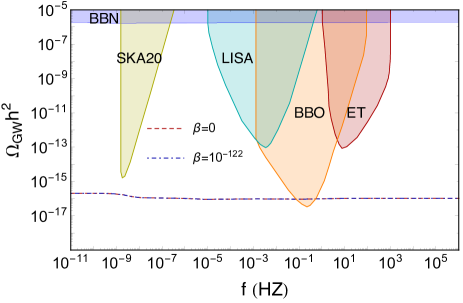
Figure 8: Plot of the PGW spectrum versus the frequency $f$, for $n_{T}=0$ and $A_{S}\sim 10^{-9}$, consistently with the Planck observational constraints at the CMB scale ConPlanck . The colored regions delineate the projected sensitivities for several GW observatories Breitbach:2018ddu .

V.2 Zero-point length Cosmology

We now study implications of the zero-point length for the PGW spectrum. Toward this end, we make use of the modified Friedmann equation (38) and the relation (102). Following Bernal:2020ywq , we can write from Eq. (100)

$$\Omega_{\mathrm{GW}}(\tau,k) \simeq \left[\frac{a_{hc}}{a(\tau)}\right]^{4}\left[\frac{H_{hc}}{H_{\mathrm{GR}}(\tau)}\right]^{2}\left[\frac{H_{\mathrm{GR}}(\tau)}{H(\tau)}\right]^{2}\frac{P_{T}(k)}{24}$$

$$=\,\Omega^{\mathrm{GR}}_{\mathrm{GW}}(\tau,k)\left[\frac{H_{\mathrm{GR}}(\tau)}{H(\tau)}\right]^{2}\left[\frac{a_{hc}}{a_{hc}^{GR}}\right]^{4}\left[\frac{a^{GR}(\tau)}{a(\tau)}\right]^{4}\left[\frac{H_{hc}}{H_{hc}^{GR}}\right]^{2}\,,$$

with

$$k\ =\ a_{\mathrm{hc}}^{\mathrm{GR}}H^{\mathrm{GR}}(a_{\mathrm{hc}}^{\mathrm{GR}})\,.$$ (107)

Here, standard quantities in General Relativity have been denoted by GR, e.g., $\Omega^{\mathrm{GR}}_{\mathrm{GW}}(\tau,k)$ is the PGW relic density

Next, using the flatness condition $H(z)/H_{0}=1$, we obtain

$$\Omega_{\mathrm{GW}}(\tau_{0},k)\ \simeq\ \Omega^{\mathrm{GR}}_{\mathrm{GW}}(\tau_{0},k)\left[\frac{a_{hc}}{a_{hc}^{GR}}\right]^{4}\left[\frac{H_{hc}}{H_{hc}^{GR}}\right]^{2}\,.$$ (108)

The modified PGW spectrum for $\beta\sim\mathcal{O}(10^{-122})$ (blue dot-dashed line) is plotted in Fig. 8. Unfortunately, if the zero-point length is around the Planck scale, no significant deviation from GR (red dashed curve) could be detected in upcoming GW observatories, at least up to frequencies around $10^{-3}\,\mathrm{GHz}$. Nevertheless, it is interesting to note that appreciable effects might still be observed in the frequency range $f\gtrsim 10^{-4}\,\mathrm{GHz}$, provided that $\beta\gtrsim 10^{-104}$ ($l_{0}\gtrsim 10^{9}$) (green dot-dashed curve in Fig. 9). If, on the one hand, this range of $\beta$ values does not fit the constraint set above through the inflation measurements, on the other hand it could be understood by allowing for a running zero-point length parameter. Although not contemplated in the original model, such a scale-dependent behavior would be fully justified, as it is consistent with the typical case occurring in quantum field theory and quantum gravity under renormalization group applications, where all parameters and coupling constants are dynamical in tandem with the energy scale. Moreover, the coupling constant in conventional quantum gravity decreases with increasing distance, in such a way that the larger the distance scale, the smaller the coupling, and vice-versa (cf. e.g. Hooft ). Notice that a similar framework has been investigated in Petroz assuming a fluctuating minimal length in the Generalized Uncertainty Principle, and in Runde by setting a varying exponent in Barrow holographic dark energy. Clearly, such a scenario may open up the possibility of new physics to be tested through future measurements of high-frequency GWs above the LIGO/VIRGO range. This analysis goes beyond the scope of the present work and will be explored elsewhere.

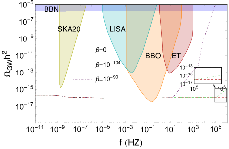
Figure 9: Plot of the PGW spectrum versus the frequency $f$ for various values of $\beta$, $n_{T}=0$ and $A_{S}\sim 10^{-9}$, consistently with the Planck observational constraints at the CMB scale ConPlanck . The colored regions delineate the projected sensitivities for several GW observatories Breitbach:2018ddu .

Moreover, a zero-point length exceeding $l_{0}\simeq 10^{16}$ ($\beta\simeq 10^{-90}$, purple dot-dashed curve in Fig. 9) appears disfavored (although not yet excluded) in our model, since it would entail a dramatic departure from GR for even GWs below $10\,\mathrm{KHz}$. This prediction is somehow consistent with the experimental evidence from particle physics LHC (we remind that subatomic distances have been directly measured up to $10^{-18}\,\mathrm{m}$ and beyond, corresponding to length scales $l\simeq 10^{17}$ in our units). The same rapid increase of the PGW spectrum at low-frequencies has been exhibited in extended scalar-tensor and extradimensional gravity Bernal:2020ywq .

VI Discussion and Conclusions

An approach to overcome the singularity problem in black hole physics is using string inspired T-duality model. In this method one can remove the singularity at the center of black hole by taking into account a zero-point length in the gravitational potential, which come from momentum space propagator induced by the path integral duality td1 . Based on this, in the present paper we have explored the effects of the zero-point length in the cosmological setup. We first derived the modified Friedmann equations due to zero-point length by applying the first law of thermodynamics on the apparent horizon. Then, we have explored the cosmological consequences of this model and disclosed the influences of the zero-point length on the history of the Universe in both the matter and radiation dominated era. The next effort has been devoted to slow-roll solutions for power-law inflation. Comparison of the slow-roll parameters with the observational values has given the constraint $l_{0}\lesssim\mathcal{O}(10^{-1}\div 1)$, depending on the expected-inflation duration. This is consistent with the original assumption Padm and the recent result in quantum corrected black holes from String T-Duality td1 .

Using the Top-Hat Spherical Collapse model, we have explored the impact on the growth of matter fluctuations in the linear regime. In spite of this minimal assumption, it has been shown that the zero-point length affects the evolution of the density contrast in a non-trivial way, leading to a slower growth of the primordial seed fluctuations into cosmic structures. In this context, we have also analyzed implications for the power spectrum of scalar perturbations. Although the simplest (and statistically preferred) inflationary models predict almost purely adiabatic perturbations with a power-law spectrum, a better observational fit is obtained by either assuming a running spectral index or different functional forms deBlas . We have found that our model naturally fits the broken-power-law (88), where the role of the $\delta$-shift is played by the zero-point length correction (see Eq. (92)).

We have finally studied the spectrum of primordial gravitational waves in the early Universe. Although Planck scale corrections to GR are hardly detectable in the near future, non-trivial effects might still be observed at frequencies accessible to the next generation GW experiments if $l_{0}\gtrsim 10^{9}$. Such a scenario is not that speculative, as it could be understood within the context of a dynamical, energy-scale-dependent behavior for the zero-point length. This would align with the typical case observed in quantum field theory and quantum gravity under renormalization group considerations (see, e.g. Hooft )..

Further aspects are yet to be investigated. First, we would like to relax our leading order assumption (19) and possibly develop exact analytical computations. This is essential for a thorough application of our model to the Planck era, which could provide hints toward the formulation of a modified Cosmology in full quantum gravity. Additionally, it would be suggestive to adapt the analysis of Sec. III to different inflationary models. A paradigmatic case is the Starobinsky inflation (and related generalizations) Staro , which is largely studied, for instance, for the theory of the origin of the Universe from a quantum multiverse Multiv .

On the other hand, recent advancements in GW experiments offer a fresh perspective on the nature of gravity in the early Universe. By probing different cosmic scales, these experiments provide a window into potential modifications to Einstein’s theory of gravity. For instance, once we detect PGWs, we will gain valuable insights that could help narrow down the parameter space for possible modifications to GR during the early Universe. While the present effort provides a preliminary analysis in this area, it is crucial to emphasize that a detailed comparison of various laboratory/astrophysical gravity tests with PGW detection appears essential. Work is in progress in this direction and will be presented elsewhere.

The era between the end of inflation and the onset of radiation domination in the Universe remains largely unexplored, and there are several UV-complete scenarios that suggest nonstandard Cosmology or modifications to gravity. In this sense, the timing of our study is very pertinent, as the next generation of GW observatories will cover several decades of frequency ranges of various GW amplitudes, allowing for the possibility to uncover new physics related to the pre-BBN era.

- (1) T. Jacobson, Phys. Rev. Lett. 75 1260 (1995).
- (2) T. Padmanabhan, Phys. Rept. 406, 49 (2005).
- (3) T. Padmanabhan, Rept. Prog. Phys. 73 046901 (2010).
- (4) A. Paranjape, S. Sarkar, T. Padmanabhan, Phys. Rev. D 74, 104015 (2006).
- (5) R. G. Cai and S. P. Kim, JHEP 02, 050 (2005).
- (6) M. Akbar and R. G. Cai, Phys. Rev. D 75, 084003 (2007).
- (7) B. Wang, Y. Gong and E. Abdalla, Phys. Rev. D 74, 083520 (2006).
- (8) A. Sheykhi, B. Wang and R. G. Cai, Nucl. Phys. B 779, 1 (2007).
- (9) A. Sheykhi, B. Wang and R. G. Cai, Phys. Rev. D 76, 023515 (2007).
- (10) A. Sheykhi, Class. Quantum Grav. 27, 025007 (2010).
- (11) E. Ayon-Beato, A. Garcia, Phys. Rev. Lett. 80 5056 (1998).
- (12) E. Ayon-Beato, A. Garcia, Phys. Lett. B 493, 149 (2000).
- (13) P. Nicolini, A. Smailagic, E. Spallucci, Phys. Lett. B 632 547 (2006).
- (14) P. Nicolini, Int. J. Mod. Phys. A 24 1229 (2009).
- (15) P. Nicolini, E. Spallucci, Class. Quant. Gravit. 27, 015010 (2010).
- (16) P. Nicolini, E. Winstanley, J. High Energy Phys. 11, 075 (2011). .
- (17) L. Modesto, J.W. Moffat, P. Nicolini, Phys. Lett. B 695 397 (2011).
- (18) T. Padmanabhan, Phys. Rev. Lett. 78 1854 (1997).
- (19) A. Smailagic, E. Spallucci, T. Padmanabhan, [arXiv:hep-th /0308122].
- (20) E. Spallucci, M. Fontanini, [arXiv:gr-qc/0508076].
- (21) M. Fontanini, E. Spallucci, T. Padmanabhan, Phys. Lett. B 633, 627 (2006).
- (22) P. Nicolini, E. Spallucci and M. F. Wondrak, Phys. Lett. B 797, 134888 (2019).
- (23) E. P. Verlinde, JHEP 1104, (2011) 029.
- (24) K. Jusufi and A. Sheykhi, Phys. Lett. B 836, 137621 (2023).
- (25) C. Tsallis and L. J. L. Cirto, Eur. Phys. J. C 73, 2487 (2013).
- (26) J. D. Barrow, Phys. Lett. B 808, 135643 (2020).
- (27) P. Jizba, G. Lambiase, G. G. Luciano and L. Petruzziello, Phys. Rev. D 105, L121501 (2022).
- (28) S. Nojiri, S. D. Odintsov and E. N. Saridakis, Eur. Phys. J. C 79, 242 (2019).
- (29) R. G. Cai, L. M. Cao and Y. P. Hu, JHEP 08, 090 (2008).
- (30) N. Komatsu, Eur. Phys. J. C 77, 229 (2017).
- (31) M. de Cesare and G. Gubitosi, JCAP 01, 046 (2024).
- (32) A. Vilenkin, Phys. Rev. D 37, 888 (1988).
- (33) A. Ashtekar and P. Singh, Class. Quant. Grav. 28, 213001 (2011).
- (34) S. Weinberg, Phys. Rev. D 72, 043514 (2005).
- (35) M. Bojowald, Phys. Rev. Lett. 86, 5227-5230 (2001).
- (36) A. Ashoorioon and R. B. Mann, Can. J. Phys. 84, 481-491 (2006).
- (37) M. V. Battisti and G. Montani, Int. J. Mod. Phys. A 23, 1257-1265 (2008).
- (38) B. Vakili, Int. J. Mod. Phys. D 18, 1059-1071 (2009).
- (39) A. F. Ali and B. Majumder, Class. Quant. Grav. 31, 215007 (2014).
- (40) S. Jalalzadeh, S. M. M. Rasouli and P. V. Moniz, Phys. Rev. D 90, 023541 (2014).
- (41) P. Bosso and O. Obregón, Class. Quant. Grav. 37, 045003 (2020).
- (42) M. F. Gusson, A. O. O. Gonçalves, R. G. Furtado, J. C. Fabris and J. A. Nogueira, Eur. Phys. J. C 81, 336 (2021).
- (43) G. G. Luciano, Eur. Phys. J. C 81, 1086 (2021).
- (44) G. G. Luciano and J. Gine, Phys. Lett. B 833, 137352 (2022).
- (45) G. G. Luciano, Eur. Phys. J. C 81, 672 (2021).
- (46) P. Nicolini, Gen. Rel. Grav. 54, 106 (2022).
- (47) P. Gaete, K. Jusufi and P. Nicolini, Phys. Lett. B 835, 137546 (2022).
- (48) S. Banerjee, R. K. Gupta, I. Mandal and A. Sen, JHEP 11, 143 (2011).
- (49) R. K. Kaul and P. Majumdar, Phys. Rev. Lett. 84, 5255-5257 (2000).
- (50) S. Carlip, Class. Quant. Grav. 17, 4175-4186 (2000).
- (51) R. J. Adler, P. Chen and D. I. Santiago, Gen. Rel. Grav. 33, 2101-2108 (2001)
- (52) S. N. Solodukhin, Living Rev. Rel. 14, 8 (2011).
- (53) A. Alonso-Serrano and M. Liška, Phys. Rev. D 108, 084057 (2023).
- (54) A. Sheykhi, Eur. Phys. J. C 69, 265-269 (2010).
- (55) A. Sheykhi, Phys. Rev. D 87, 061501 (2013).
- (56) S. A. Hayward, Class. Quant. Grav. 15, 3147 (1998).
- (57) A. G. Riess et al. [Supernova Search Team], Astron. J. 116, 1009 (1998).
- (58) D. H. Weinberg, M. J. Mortonson, D. J. Eisenstein, C. Hirata, A. G. Riess and E. Rozo, Phys. Rept. 530, 87 (2013).
- (59) D. J. Eisenstein et al. [SDSS], Astrophys. J. 633, 560-574 (2005).
- (60) S. Capozziello, R. D’Agostino and O. Luongo, Mon. Not. Roy. Astron. Soc. 494, 2576-2590 (2020).
- (61) D. M. Naik, N. S. Kavya, L. Sudharani and V. Venkatesha, Eur. Phys. J. C 83, 840 (2023).
- (62) S. Weinberg, Gravitation and cosmology, John Wiley & Sons Inc, Ne. Yo. (1972).
- (63) M. Visser, Class. Quant. Grav. 21, 2603 (2004).
- (64) D. Rapetti, S. W. Allen, M. A. Amin and R. D. Blandford, Mon. Not. Roy. Astron. Soc. 375, 1510-1520 (2007).
- (65) R. D. Blandford, M. A. Amin, E. A. Baltz, K. Mandel and P. J. Marshall, ASP Conf. Ser. 339, 27 (2005).
- (66) S. Capozziello, O. Farooq, O. Luongo and B. Ratra, Phys. Rev. D 90, 044016 (2014).
- (67) S. Pan, A. Mukherjee and N. Banerjee, Mon. Not. Roy. Astron. Soc. 477, 1189-1205 (2018).
- (68) G. G. Luciano, Eur. Phys. J. C 83, 329 (2023).
- (69) A. I. Keskin, Int. J. Geom. Meth. Mod. Phys. 19, 2250005 (2022).
- (70) S. D. Odintsov and V. K. Oikonomou, JCAP 04, 041 (2017).
- (71) G.N. Remmen, S.M. Carroll, Phys. Rev. D 90, 063517 (2014).
- (72) A.R. Liddle, S.M. Leach, Phys. Rev. D 68, 103503 (2003).
- (73) P. W. Graham and A. Scherlis, Phys. Rev. D 98, 035017 (2018).
- (74) S. Y. Ho, F. Takahashi and W. Yin, JHEP 04, 149 (2019).
- (75) P. W. Graham, D. E. Kaplan and S. Rajendran, Phys. Rev. Lett. 115, 221801 (2015).
- (76) C. Ringeval, T. Suyama, T. Takahashi, M. Yamaguchi and S. Yokoyama, Phys. Rev. Lett. 105, 121301 (2010).
- (77) N. Kitajima, Y. Tada and F. Takahashi, Phys. Lett. B 800, 135097 (2020).
- (78) A. R. Liddle, Phys. Lett. B 220, 502-508 (1989).
- (79) P. Campeti and E. Komatsu, Astrophys. J. 941, 110 (2022).
- (80) W. Giarè, S. Pan, E. Di Valentino, W. Yang, J. de Haro and A. Melchiorri, JCAP 09, 019 (2023).
- (81) M. Alhallak, N. Chamoun and M. S. Eldaher, Eur. Phys. J. C 83, 533 (2023).
- (82) S. Nojiri, S. D. Odintsov and V. K. Oikonomou, Phys. Rept. 692, 1-104 (2017).
- (83) E. Di Valentino and L. Mersini-Houghton, JCAP 03, 020 (2017).
- (84) R. Adhikari, M. R. Gangopadhyay and Yogesh, Eur. Phys. J. C 80, 899 (2020).
- (85) F. Lucchin and S. Matarrese, Phys. Rev. D 32, 1316 (1985).
- (86) G. Lambiase, G. G. Luciano and A. Sheykhi, Eur. Phys. J. C 83, 936 (2023).
- (87) V. F. Mukhanov, H. A. Feldman and R. H. Brandenberger, Phys. Rept. 215, 203-333 (1992).
- (88) K. A. Malik and D. Wands, Phys. Rept. 475, 1-51 (2009).
- (89) L. R. Abramo, R. C. Batista, L. Liberato and R. Rosenfeld, JCAP 11, 012 (2007).
- (90) S. Planelles, D. R. G. Schleicher and A. M. Bykov, Space Sci. Rev. 188, 93-139 (2015).
- (91) H. Hamber and R. Toriumi, Galaxies 2, 275-291 (2014).
- (92) G. M. Hossain, Class. Quant. Grav. 22, 2511-2532 (2005).
- (93) S. Carloni, P. K. S. Dunsby and A. Troisi, Phys. Rev. D 77, 024024 (2008).
- (94) S. Gielen and D. Oriti, Phys. Rev. D 98, 106019 (2018).
- (95) N. Aghanim et al. [Planck], Astron. Astrophys. 641, A6 (2020) [erratum: Astron. Astrophys. 652, C4 (2021)].
- (96) P. Zarrouk et al. [eBOSS], Mon. Not. Roy. Astron. Soc. 477, 1639-1663 (2018).
- (97) S. Alam et al. [BOSS], Mon. Not. Roy. Astron. Soc. 470, 2617-2652 (2017).
- (98) L. Heisenberg, H. Villarrubia-Rojo and J. Zosso, Phys. Rev. D 106, 043503 (2022).
- (99) S. Basilakos, A. Lymperis, M. Petronikolou and E. N. Saridakis, Eur. Phys. J. C 84, 297 (2024).
- (100) E. R. Harrison, Phys. Rev. D 1, 2726 (1970).
- (101) Y. B. Zeldovich, Mon. Not. Roy. Astron. Soc. 160, 1P-3P (1972).
- (102) D. M. de Blas and J. Olmedo, JCAP 06, 029 (2016).
- (103) J. Aasi et al. [LIGO Scientific], Class. Quant. Grav. 32, 074001 (2015).
- (104) F. Acernese et al. [VIRGO], Class. Quant. Grav. 32, 024001 (2015).
- (105) A. Ito and J. Soda, Eur. Phys. J. C 83, 766 (2023).
- (106) Y. Watanabe and E. Komatsu, Phys. Rev. D 73, 123515 (2006).
- (107) S. Weinberg, Phys. Rev. D 69, 023503 (2004).
- (108) N. Bernal, A. Ghoshal, F. Hajkarim and G. Lambiase, JCAP 11, 051 (2020).
- (109) M. C. Guzzetti, N. Bartolo, M. Liguori and S. Matarrese, Riv. Nuovo Cim. 39, 399-495 (2016).
- (110) Y. Akrami et al. [Planck], Astron. Astrophys. 641, A10 (2020).
- (111) M. Breitbach, J. Kopp, E. Madge, T. Opferkuch and P. Schwaller, JCAP 07, 007 (2019).
- (112) G. Janssen, G. Hobbs, M. McLaughlin, C. Bassa, A. T. Deller, M. Kramer, K. Lee, C. Mingarelli, P. Rosado and S. Sanidas, et al. PoS AASKA14, 037 (2015).
- (113) P. Amaro-Seoane et al. [LISA], [arXiv:1702.00786 [astro-ph.IM]].
- (114) B. Sathyaprakash, M. Abernathy, F. Acernese, P. Ajith, B. Allen, P. Amaro-Seoane, N. Andersson, S. Aoudia, K. Arun and P. Astone, et al. Class. Quant. Grav. 29, 124013 (2012) [erratum: Class. Quant. Grav. 30, 079501 (2013)].
- (115) J. Crowder and N.J. Cornish, Phys. Rev. D 72, 083005 (2005).
- (116) L.A. Boyle and A. Buonanno, Phys. Rev. D 78, 043531 (2008).
- (117) A. Stewart and R. Brandenberger, JCAP 08, 012 (2008).
- (118) G. ’t Hooft, Nucl. Phys. B 256, 727 (1985).
- (119) L. Petruzziello and F. Illuminati, Nature Commun. 12, 4449 (2021).
- (120) S. Basilakos, A. Lymperis, M. Petronikolou and E. N. Saridakis, [arXiv:2312.15767 [gr-qc]].
- (121) P. A. Zyla et al. [Particle Data Group], PTEP 2020, 083C01 (2020).
- (122) A. A. Starobinsky, Phys. Lett. B 91, 99-102 (1980).
- (123) L. Mersini-Houghton, Class. Quant. Grav. 34, 047001 (2017).