Exploiting New Properties of String Net Frequency for Efficient Computation

Abstract

Knowing which strings in a massive text are significant – that is, which strings are common and distinct from other strings – is valuable for several applications, including text compression and tokenization. Frequency in itself is not helpful for significance, because the commonest strings are the shortest strings. A compelling alternative is net frequency, which has the property that strings with positive net frequency are of maximal length. However, net frequency remains relatively unexplored, and there is no prior art showing how to compute it efficiently. We first introduce a characteristic of net frequency that simplifies the original definition. With this, we study strings with positive net frequency in Fibonacci words. We then use our characteristic and solve two key problems related to net frequency. First, single-nf, how to compute the net frequency of a given string of length $m$, in an input text of length $n$ over an alphabet size $\sigma$. Second, all-nf, given length-$n$ input text, how to report every string of positive net frequency (and its net frequency). Our methods leverage suffix arrays, components of the Burrows-Wheeler transform, and solution to the coloured range listing problem. We show that, for both problems, our data structure has $\text{O}(n)$ construction cost: with this structure, we solve single-nf in $\text{O}(m+\sigma)$ time and all-nf in $\text{O}(n)$ time. Experimentally, we find our method to be around 100 times faster than reasonable baselines for single-nf. For all-nf, our results show that, even with prior knowledge of the set of strings with positive net frequency, simply confirming that their net frequency is positive takes longer than with our purpose-designed method. All in all, we show that net frequency is a cogent method for identifying significant strings. We show how to calculate net frequency efficiently, and how to report efficiently the set of plausibly significant strings.

1 Introduction

When analysing, storing, manipulating, or working with text, identification of notable (or significant) strings is typically a key component. These notable strings could form the basis of a dictionary for compression, be exploited by a tokenizer, or form the basis of trend detection. Here, a text is a sequence of characters drawn from a fixed alphabet, such as a book, collection of articles, or a Web crawl. A string is a contiguous sub-sequence of the text; in this paper, we seek to efficiently identify notable strings.

Given a text, $T$, and a string, $S$, the frequency of $S$ is the number of occurrences of $S$ in $T$. The frequency of a string is inherently a basis for its significance. However, frequency is in some sense uninformative. Sometimes a shorter string is frequent only because it is part of many different longer strings, or of a frequent longer string, or of many frequent longer strings. That is, the frequency of a string may be inflated by the occurrences of the longer strings that contain it. Moreover, every substring of a string of frequency $f$ has frequency at least $f$. Indeed, the most frequent string in the text has length $1$.

A compelling means of identifying notable strings is via net frequency (NF), introduced by Lin and Yu [23]. Let $T=\texttt{r\hbox{\pagecolor{lightgray!40}\vrule width=0.0pt,height=0.0pt,depth=0.0ptst\/}k\text@underline{\hbox{\pagecolor{lightgray!40}\vrule width=0.0pt,height=0.0pt,depth=0.0ptst\/}}ca\hbox{\pagecolor{lightgray!40}\vrule width=0.0pt,height=0.0pt,depth=0.0ptst\/}ar\hbox{\pagecolor{lightgray!40}\vrule width=0.0pt,height=0.0pt,depth=0.0ptst\/}a\hbox{\pagecolor{lightgray!40}\vrule width=0.0pt,height=0.0pt,depth=0.0ptst\/}\$}$ be an input text. The highlighted string st has frequency five. But to arrive at a more helpful notion of the frequency of the string st, the occurrences of st in repeated longer strings – that is, rst and ast – should be excluded, leaving one occurrence left (underlined). Defined precisely in Section 3, net frequency (NF) captures this idea; indeed, the NF of st in $T$ is $1$. For now, strings with positive NF are those that are repeated in the text and are maximal (see Theorem 3.3, below): if extended to either left or right the frequency of the extended string would be $1$. For the underlined st above, the frequency of both kst (left) and stc (right) is $1$.

It is worth noting the difference between a string with positive NF and a maximal repeat [21, 33, 35]: when extending a string with positive NF, the frequency of the extended string becomes 1, whereas when extending a maximal repeat, the frequency of the extended string decreases, but does not necessarily become 1.

Motivation.

NF has been demonstrated to be useful in tasks such as Chinese phoneme-to-character (and character-to-phoneme) conversion, the determination of prosodic segments in a Chinese sentence for text-to-speech output, and Chinese toneless phoneme-to-character conversion for Chinese spelling error correction [23, 24]. NF could also be complementary to tasks such as parsing in NLP and structure discovery in genomic strings. However, even though the original paper on NF [23] suggested that “suitable indexing can be used to improve efficiency”, efficient structures and algorithms for NF were not explicitly described. In this work, we bridge this gap by delving into the properties of NF. Through these properties, we introduce efficient algorithms for computing NF.

Problem definition.

Throughout, $T$ is our length-$n$ input text and $S$ a length-$m$ string in $T$. We consider two problems relating to computing NF in $T$: the Single-string Net Frequency problem single-nf and the All-strings Net Frequency problem all-nf:

• single-nf: given a text, $T$, and a query string, $S$, report the NF of $S$ in $T$.

• all-nf: given a text, $T$, identify each string that has positive NF in $T$. Concretely, the identification could be one of the following two forms. all-nf-report: for each string of positive NF, report one occurrence and its NF; or all-nf-extract: extract a multiset, where each element is a string with positive NF and its multiplicity is its NF.

Our contribution.

In this work, we first reconceptualise NF through our new characteristic that simplifies the original definition. We then apply it and identify strings with positive NF in Fibonacci words. For single-nf, we introduce an $\text{O}(m+\sigma)$ time algorithm, where $m$ is the length of the query and $\sigma$ is the size of the alphabet. This is achieved via several augmentation to suffix array from LF mapping to LCP array, as well as solution to the coloured range listing problem. For all-nf, we establish a connection to branching strings and LCP intervals, then solve all-nf-report in $\text{O}(n)$ time, and all-nf-extract in $\text{O}(n\log\delta)$ time, where $\delta$ is a repetitiveness measure defined as $\delta:=\max\left\{S(k)/k:k\in[n]\right\}$ and $S(k)$ denotes the number of distinct strings of length $k$ in $T$. The cost is bounded by making a connection to irreducible LCP values. We also conducted extensive experiments and demonstrated the efficiency of our algorithms empirically. The code for our experiments is available at https://github.com/peakergzf/string-net-frequency.

2 Preliminaries

Strings.

Let $\Sigma$ be a finite alphabet of size $\sigma$. Given a character, $x$, and two strings, $S$ and $T$, some of their possible concatenations are written as $xS$, $Sx$, $\mathit{ST}$, and $\mathit{TS}$. If $S$ is a substring of $T$, we write $S\prec T$ or $T\succ S$. Let $[n]$ denote the set $\{1,2,\ldots,n\}$. A substring of $T$ with starting position $i\in[n]$ and end position $j\in[n]$ is written as $T[i\ldots j]$. A substring $T[1\ldots j]$ is called a prefix of $T$, and $T[i\ldots n]$ is called a suffix of $T$. Let $T_{i}$ denote the $i^{\text{th}}$ suffix of $T$, $T[i\ldots n]$. An occurrence in the text $T$ is a pair of starting and ending positions $(s,e)\in[n]\times[n]$. We say $(s,e)$ is an occurrence of string $S$ if $S=T[s\ldots e]$, and $i$ is an occurrence of $S$ if $S=T[i\ldots i+|S|-1]$. The frequency of $S$, denoted by $f(S)$, is the number of occurrences of $S$ in $T$. A string $S$ is unique if $f(S)=1$ and is repeated if $f(S)\geq 2$.

Suffix arrays and Burrows-Wheeler transform.

The suffix array (SA) [27] of $T$ is an array of size $n$ where $\mathit{SA}[i]$ stores the text position of the $i^{\text{th}}$ lexicographically smallest suffix. For a string $S$, let $l$ and $r$ be the smallest and largest positions in $\mathit{SA}$, respectively, where $S$ is a prefix of the corresponding suffixes $T_{\mathit{SA}[l]}$ and $T_{\mathit{SA}[r]}$. Then, the closed interval $\langle l,r\rangle$ is referred to as the SA interval of $S$. The inverse suffix array (ISA) of a suffix array $\mathit{SA}$ is an array of length $n$ where $\mathit{ISA}[i]=j$ if and only if $\mathit{SA}[j]=i$. The Burrows-Wheeler transform (BWT) [29] of $T$ is a string of length $n$ where $\mathit{BWT}[i]=T[\mathit{SA}[i]-1]$ for $\mathit{SA}[i]>1$ and $\mathit{BWT}[i]=\$$ if $\mathit{SA}[i]=1$. The LF mapping is an array of length $n$ where $\mathit{LF}[i]=\mathit{ISA}[\mathit{SA}[i]-1]$ for $\mathit{SA}[i]>1$, and $\mathit{LF}[i]=1$ if $\mathit{SA}[i]=1$.

LCP arrays and irreducible LCP values.

The longest common prefix array (LCP) [17, 28] is an array of length $n$ where the $i^{\text{th}}$ entry in the LCP array stores the length of the longest common prefix between $T_{\mathit{SA}[i-1]}$ and $T_{\mathit{SA}[i]}$, which is denoted $\mathit{lcp}\left(T_{\mathit{SA}[i-1]},T_{\mathit{SA}[i]}\right)$. An entry $\mathit{LCP}[i]$ is called reducible if $\mathit{BWT}[i-1]=\mathit{BWT}[i]$ and irreducible otherwise. The sum of irreducible LCP values was first bounded as $\text{O}(n\log n)$ [16]. Later the bound has been refined with the development of repetitiveness measures [31]. Let $r$ be the number of equal-letter runs in the BWT of $T$. The bound on the sum of irreducible LCP values was improved [15] to $\text{O}(n\log r)$. Let $S(k)$ be the number of distinct strings of length $k$ in $T$, and define $\delta:=\max\left\{S(k)/k:k\in[n]\right\}$ [6, 20, 36]. The bound was further improved in the following result.

Lemma 2.1 ([18]).

The sum of irreducible LCP values is at most $\text{O}(n\log\delta)$.

Coloured range listing.

The coloured range listing (CRL) problem is defined as follows. Preprocess a text $T$ of length $n$ such that, later, given a range $i,\ldots,j$, list the position of each distinct character (“colour”) in $T[i\ldots j]$. The data structure introduced in [30] lists each such position in $\text{O}(1)$ time, occupying $\text{O}(n\log n)$ bits of space. Compressed structures for the CRL problem have also been introduced [10].

3 A Fresh Examination of Net Frequency

In this section, we lay the foundation for efficient net frequency (NF) computation by re-examining NF and proving several properties. Before we formally define NF, we first introduce the notion of extensions.

Definition 3.1 (Extensions).

Given a string $S$ and two symbols $x,y\in\Sigma$, strings $xS$, $Sy$, and $xSy$ are called the left, right, and bidirectional extension of $S$, respectively. A left or right extension is also called a unidirectional extension. We then define the following sets of extensions: $L(S):=\left\{x\in\Sigma:f(xS)\geq 2\right\},R(S):=\left\{y\in\Sigma:f(Sy)\geq 2\right\},\text{\leavevmode\nobreak\ and\leavevmode\nobreak\ }B(S):=\left\{(x,y)\in L(S)\times R(S):f(xSy)\geq 1\right\}.$

Note that the definition of $B(S)$ does not require that string $xSy$ needs to repeat; only the unidirectional extensions, $xS$ and $Sy$, must do so.

Definition 3.2 (Net frequency [23]).

Given a string $S$ in $T$, the NF of $S$ is zero if it is unique in $T$; otherwise $S$ repeats and the NF of $S$ is defined as

$$\mathit{\phi}(S):=f(S)-\sum_{x\in L(S)}f(xS)-\sum_{y\in R(S)}f(Sy)+\sum_{(x,y)\in B(S)}f(xSy)\,.$$

The two subtraction terms discount the occurrences that are part of longer repeated strings while the addition term compensates for double counting (occurrences of $xS$ and $Sy$ could correspond to the same occurrence of $S$), an inclusion-exclusion approach. We now introduce a fresh examination of NF that significantly simplifies the original definition and will be the backbone of our algorithms for NF computation later.

Theorem 3.3 (Net frequency characteristic).

Given a repeated string $S$,

$$\mathit{\phi}(S)=\left|\left\{\,(x,y)\in\Sigma\times\Sigma:f(xS)=1\text{\leavevmode\nobreak\ and\leavevmode\nobreak\ }f(Sy)=1\text{\leavevmode\nobreak\ and\leavevmode\nobreak\ }f(xSy)=1\,\right\}\right|\,.$$

Proof 3.4.

We first define the following sets:

$$L^{+}(S) :=\{(x,y)\in\Sigma\times\Sigma:f(xS)\geq 2\text{\leavevmode\nobreak\ and\leavevmode\nobreak\ }f(Sy)=1\},$$

$$R^{+}(S) :=\{(x,y)\in\Sigma\times\Sigma:f(xS)=1\text{\leavevmode\nobreak\ and\leavevmode\nobreak\ }f(Sy)\geq 2\},\text{\leavevmode\nobreak\ and\leavevmode\nobreak\ }$$

$$U(S) :=\{(x,y)\in\Sigma\times\Sigma:f(xS)=1\text{\leavevmode\nobreak\ and\leavevmode\nobreak\ }f(Sy)=1\}.$$

For convenience, we define

$$F(W):=\sum_{(x,y)\in W(S)}f(xSy)\quad\text{where}\quad W\in\{B,L^{+},R^{+},U\}.$$

Then, we have $f(S)=F(L^{+})+F(B)+F(R^{+})+F(U)$. Also note that

$$\sum_{x\in L(S)}f(xS)=F(L^{+})+F(B)\quad\text{and}\quad\sum_{y\in R(S)}f(Sy)=F(R^{+})+F(B).$$

Substituting these to Definition 3.2, we have

$$\mathit{\phi}(S)=\left(F(L^{+})+F(B)+F(R^{+})+F(U)\right) -\left(F(L^{+})+F(B)\right)$$

$$-\left(F(R^{+})+F(B)\right)+F(B)=F(U).$$

Finally, observe that $F(U)$ equals to the expression in Theorem 3.3 since when $f(xS)=1$ and $f(Sy)=1$, $f(xSy)$ can only be 0 or 1.

In the original definition of NF and in our characteristics, extensions are limited to adding only one character to one side of the string. It is intriguing to explore the impact of longer extensions. Surprisingly, the analogous quantity of NF with longer extensions is equal to NF.

Lemma 3.5.

Given a repeated string $S$, for each $k\geq 1$, we have $\mathit{\phi}(S)=\mathit{\phi}_{k}(S)$ where

$$\mathit{\phi}_{k}(S):=\left|\left\{\,(X,Y)\in\Sigma^{k}\times\Sigma^{k}:f(XS)=1\text{\leavevmode\nobreak\ and\leavevmode\nobreak\ }f(SY)=1\text{\leavevmode\nobreak\ and\leavevmode\nobreak\ }f(XSY)=1\,\right\}\right|\,.$$

Proof 3.6.

First note that $\mathit{\phi}_{1}(S)=\mathit{\phi}(S)$ by Theorem 3.3. We then aim to show that for each $k>1$, $\mathit{\phi}_{k}(S)=\mathit{\phi}_{k+1}(S)$. For convenience, we express $\mathit{\phi}_{k}$ in the following summation. Note that we do not need the condition $f(XSY)=1$ because it is either 0 or 1 for each summand.

$$\mathit{\phi}_{k}(S)=\sum_{(X,Y)\in\Sigma^{k}\times\Sigma^{k}}^{\begin{subarray}{c}f(XS)=1\\ f(SY)=1\end{subarray}}f(XSY).$$

Next, observe that for any string $S$, its frequency can be expressed using the frequencies of the bidirectional extensions of $S$:

$$f(S)=\sum_{(a,b)\in\Sigma\times\Sigma}f(aSb).$$

We then substitute $f(XSY)$ in $\mathit{\phi}_{k}(S)$ using the above equality:

$$\mathit{\phi}_{k}(S)=\sum_{(X,Y)\in\Sigma^{k}\times\Sigma^{k}}^{\begin{subarray}{c}f(XS)=1\\ f(SY)=1\end{subarray}}\sum_{(a,b)\in\Sigma\times\Sigma}f(aXSYb).$$

For the inner summation, observe that $f(aXS)\leq f(XS)=1$ and $f(SYb)\leq f(SY)=1$, thus,

$$\mathit{\phi}_{k}(S)=\sum_{(X,Y)\in\Sigma^{k}\times\Sigma^{k}}^{\begin{subarray}{c}f(XS)=1\\ f(SY)=1\end{subarray}}\sum_{(a,b)\in\Sigma\times\Sigma}^{\begin{subarray}{c}f(aXS)=1\\ f(SYb)=1\end{subarray}}f(aXSYb)=\sum_{(aX,Yb)\in\Sigma^{k+1}\times\Sigma^{k+1}}^{\begin{subarray}{c}f(aXS)=1\\ f(SYb)=1\end{subarray}}f(aXSYb).$$

Let $X^{\prime}:=aX$ and $Y^{\prime}:=Yb$, we have

$$\mathit{\phi}_{k}(S)=\sum_{(X^{\prime},Y^{\prime})\in\Sigma^{k+1}\times\Sigma^{k+1}}^{\begin{subarray}{c}f(X^{\prime}S)=1\\ f(SY^{\prime})=1\end{subarray}}f(X^{\prime}SY^{\prime})=\mathit{\phi}_{k+1}(S).$$

And therefore, we have shown that $\mathit{\phi}_{k}(S)=\mathit{\phi}(S)$ for each $k\geq 1$.

So far the definition and properties of NF have been formulated in terms of symbols from the alphabet. To facilitate our discussion on the properties and algorithms of NF later, we switch our focus away from symbols and reformulate NF in terms of occurrences. Recall that the frequency of a string $S$ is the number of occurrences of $S$. Analogously, the NF of $S$ is the number of net occurrences of $S$.

Definition 3.7 (Net occurrence).

An occurrence $(i,j)$ is a net occurrence if $f(T[i\ldots j])\geq 2$, $f(T[i-1\ldots j])=1$, and $f(T[i\ldots j+1])=1$. When $i=1$, $f(T[i-1\ldots j])=1$ is assumed to be true; when $j=n$, $f(T[i\ldots j+1])=1$ is assumed to be true.

When $f(xS)=1$ and $f(Sy)=1$, $f(xSy)$ is either 0 or 1. But when $f(T[i-1\ldots j])=1$ and $f(T[i\ldots j+1])=1$, $f(T[i-1\ldots j+1])$ must be 1 and cannot be 0. Thus, the conditions in Definition 3.7 do not mention the bidirectional extension, $f(T[i-1\ldots j+1])=1$.

3.1 Net Frequency of Fibonacci Words: A Case Study

Let $F_{i}$ be the $i^{\text{th}}$ (finite) Fibonacci word over binary alphabet $\{\texttt{a},\texttt{b}\}$, where $F_{1}:=\texttt{b},F_{2}:=\texttt{a}$, and for each $i\geq 3$, $F_{i}:=F_{i-1}F_{i-2}$. Note that $|F_{i}|=f_{i}$ where $f_{i}$ is the $i^{\text{th}}$ Fibonacci number. There has been an extensive line of research on Fibonacci words, from their combinatorial properties [19] to lower bounds and worst-case examples for strings algorithms [14]. The first ten Fibonacci words are presented in Table 1.

In this section, we examine the NF of Fibonacci words, which later will help us obtain a lower bound on the sum of lengths of strings with positive NF in a text. Specifically, we assume $i\geq 7$, we regard $F_{i}$ as our input text, and we study the net frequency of $F_{i-2}$ and $S_{i}:=F_{i-1}[1\ldots f_{i-1}-2]$ in $F_{i}$.

Table 1: The $i^{\text{th}}$ Fibonacci number $f_{i}$ and the $i^{\text{th}}$ Fibonacci word $F_{i}$ are listed for $1\leq i\leq 10$. Net occurrences in $F_{i}$ are underlined for $i\geq 7$.

$i$	$f_{i}$	$F_{i}$
1	1	b
2	1	a
3	2	ab
4	3	aba
5	5	abaab
6	8	abaababa
7	13	abaababaabaab
8	21	abaababaabaababaababa
9	34	abaababaabaababaababaabaababaabaab
10	55	abaababaabaababaababaabaababaabaababaababaabaababaababa

Net Frequency of $F_{i-2}$ in $F_{i}$

We begin by introducing some basic concepts in combinatorics on words [25]. A nonempty word $u$ is a repetition of a word $w$ if there exist words $x,y$ such that $w=xu^{k}y$ for some integer $k\geq 2$. When $k=2$, the repetition is called a square. A word $v$ that is both a prefix and a suffix of $w$, with $v\neq w$, is called a border of $w$. Stronger results on the borders and squares of $F_{i}$ have been introduced before [7, 13], but for our purposes, the following suffices.

$F_{i-2}$ is a border and a square of $F_{i}$.

Proof 3.8.

We apply the recurrence and factorise $F_{i}$ as follows. Occurrences of $F_{i-2}$ as a border or a square of $F_{i}$ are underlined. $F_{i}=F_{i-1}\ F_{i-2}=\underline{F_{i-2}}\ F_{i-3}\ \underline{F_{i-2}}=F_{i-2}\ F_{i-3}\ F_{i-3}\ F_{i-4}=F_{i-2}\ F_{i-3}\ F_{i-4}\ F_{i-5}\ F_{i-4}=\underline{F_{i-2}}\ \underline{F_{i-2}}\ F_{i-5}\ F_{i-4}.$

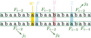
Figure 1: Illustration of proof of Theorem 3.9. Two factorisations of $F_{8}$ are depicted with rectangles.

Theorem 3.9.

$\mathit{\phi}(F_{i-2})\geq 1$.

Proof 3.10.

The proof is illustrated in Figure 1. In the following two factorisations of $F_{i}$, $F_{i}=F_{i-2}\ F_{i-3}\ F_{i-2}$ and $F_{i}=F_{i-2}\ F_{i-2}\ F_{i-5}\ F_{i-4}$, consider $j_{1},j_{2}$, and $j_{3}$, three occurrences of $F_{i-2}$. Let $w$ and $y$ be the left extension characters of $j_{2}$ and $j_{3}$, respectively, and let $x$ and $z$ be the right extension characters of $j_{1}$ and $j_{2}$, respectively. Using the factorisation $F_{i}=F_{i-2}\ F_{i-3}\ F_{i-2}$, observe that $w=F_{i-2}[f_{i-2}]$, $x=F_{i-2}[1]$, and $y=F_{i-3}[f_{i-3}]$. Using the factorisation $F_{i}=F_{i-2}\ F_{i-2}\ F_{i-5}\ F_{i-4}$, we have $z=F_{i-5}[1]$. Thus, $x=z=\texttt{a}$, and $w\neq y$ because the last character of consecutive Fibonacci words alternates. Therefore, $j_{1}$ and $j_{2}$ are not net occurrences of $F_{i-2}$ in $F_{i}$ and only $j_{3}$ is.

Net Frequency of $S_{i}$ in $F_{i}$

In the recurrence of Fibonacci word, $F_{i-2}$ is appended to $F_{i-1}$, $F_{i}=F_{i-1}\ F_{i-2}$. When we reverse the order of the concatenation and prepend $F_{i-2}$ to $F_{i-1}$, for example, notice that $F_{6}\ F_{5}=\texttt{abaababa|aba\text@underline{ab}}$ and $F_{5}\ F_{6}=\texttt{abaab|abaaba\text@underline{ba}}$ only differ in the last two characters. Such property is referred to as near-commutative in [34]. In our case, we characterise the string that is invariant under such reversion with $Q_{i}$ in the following definition.

Definition 3.11 ($Q_{i}$ and $\Delta(j)$).

Let $Q_{i}:=F_{i-5}\ F_{i-6}\cdots F_{3}\ F_{2}$ be the concatenation of $i-6$ consecutive Fibonacci words in decreasing length. For $j\in\{0,1\}$, we define $\Delta(j):=\texttt{ba}$ if $j=0$, and $\Delta(j):=\texttt{ab}$ otherwise.

In Figure 2, $F_{i-4}\ F_{i-5}$ and $F_{i-5}\ F_{i-4}$ only differ in the last two characters, and their common prefix is $Q_{i}$. The alternation between ab and ba was also observed in [8], but their focus was on capturing the length-2 suffix appended to the palindrome $F_{i}[1\ldots f_{i}-2]$.

Observe that $F_{i-3}=F_{i-4}\ F_{i-5}$, the invariant discussed earlier is captured as follows.

Lemma 3.12.

$F_{i-3}=Q_{i}\ \Delta\left(1-(i\bmod 2)\right)\quad\text{and}\quad F_{i-5}\ F_{i-4}=Q_{i}\ \Delta(i\bmod 2).$

Proof 3.13 (Proof of Lemma 3.12 (first equality)).

Let $P(i)$ be the statement $F_{i-3}=Q_{i}\ \Delta(1-(i\bmod 2))$. We prove $P(i)$ by strong induction. Base case: observe that $F_{7-3}=\texttt{aba}$, $Q_{7}=F_{2}=\texttt{a}$, and $\Delta(1-(7\bmod 2))=\Delta(0)=\texttt{ba}$. Inductive step: consider $k>7$, assume that $P(j)$ holds for every $j\leq k$. We now prove $P(k+1)$ holds. First, $F_{k-2}=F_{k-3}\ F_{k-4}=F_{k-4}\ F_{k-5}\ F_{k-4}$. Then, based on our inductive hypothesis, $F_{k-4}=Q_{k-1}\ \Delta(1-(k-1)\bmod 2)=F_{k-6}\ F_{k-7}\cdots F_{3}\ F_{2}\ \Delta(1-(k-1)\bmod 2).$ Substituting the second $F_{k-4}$ in $F_{k-2}$, we have

$$F_{k-2}=F_{k-4}\ F_{k-5}\ F_{k-6}\ F_{k-7}\cdots F_{3}\ F_{2}\ \Delta(1-(k-1)\bmod 2)=Q_{k+1}\ \Delta(1-(k+1)\bmod 2).$$

By induction, $P(i)$ holds for all $i$.

Proof 3.14 (Proof of Lemma 3.12 (second equality)).

Let $P(i)$ be the statement $F_{i-5}\ F_{i-4}=Q_{i}\ \Delta(i\bmod 2)$. We prove $P(i)$ by strong induction. Base case: observe that $F_{7-5}=\texttt{a}$, $F_{7-4}=\texttt{ab}$, $Q_{7}=F_{2}=\texttt{a}$, and $\Delta(7\bmod 2)=\Delta(1)=\texttt{ab}$. Inductive step: consider $k>7$, assume that $P(j)$ holds for every $j\leq k$. We now prove $P(k+1)$ holds. First, $F_{k-4}\ F_{k-3}=F_{k-4}\ F_{k-4}\ F_{k-5}=F_{k-4}\ F_{k-5}\ F_{k-6}\ F_{k-5}.$ Then, based on our inductive hypothesis, $F_{k-6}\ F_{k-5}=Q_{k-1}\ \Delta((k-1)\bmod 2)=F_{k-6}\ F_{k-7}\cdots F_{3}\ F_{2}\ \Delta((k-1)\bmod 2),$ which means $F_{k-5}=F_{k-7}\cdots F_{3}\ F_{2}\ \Delta((k-1)\bmod 2).$ Substituting the second $F_{k-5}$ in $F_{k-4}\ F_{k-3}$, we have

$$F_{k-4}\ F_{k-3}=F_{k-4}\ F_{k-5}\ F_{k-6}\ F_{k-7}\cdots F_{3}\ F_{2}\ \Delta((k-1)\bmod 2)=Q_{k+1}\ \Delta((k+1)\bmod 2).$$

By induction, $P(i)$ holds for all $i$.

Previously we defined $S_{i}$ as the length $(f_{i-1}-2)$ prefix of $F_{i-1}$, now we can see that this is to remove $\Delta$ ($|\Delta|=2$). With Lemma 3.12, we now present the main result on the NF of $S_{i}$.

Theorem 3.15.

$\mathit{\phi}(S_{i})\geq 2$.

Proof 3.16.

It follows from Lemma 3.12 that $F_{i-1}=F_{i-2}\ F_{i-3}=F_{i-2}\ Q_{i}\ \Delta(1-(i\bmod 2))$. Then, $S_{i}=F_{i-1}[1\ldots f_{i-1}-2]=F_{i-2}\ Q_{i}$. Consider the two occurrences of $S_{i}$, observe that the right extension characters of these occurrences are different: $\Delta(1-(i\bmod 2))[1]\neq\Delta(i\bmod 2)[1]$. (In Figure 2, $\Delta(1)[1]\neq\Delta(0)[1]$.) Therefore, both occurrences are net occurrences.

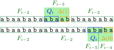
Figure 2: Illustration of Lemma 3.12 with $F_{8}$. Note that $F_{i-5}=\texttt{ab}$ and $F_{i-4}=\texttt{aba}$.

Remark 3.17.

Theorem 3.9 and Theorem 3.15 show that there are at least three net occurrences in $F_{i}$ (one of $F_{i-2}$ and two of $S_{i}$). Empirically, we have verified that these are the only three net occurrences in $F_{i}$ for each $i$ until a reasonably large $i$. Future work can be done to prove this tightness.

4 New Algorithms for Net Frequency Computation

Our reconceptualisation of NF provides a basis for computation of NF in practice. In this section, we introduce our efficient approach for NF computation.

4.1 SINGLE-NF Algorithm

To compute the NF of a query string $S$, it is sufficient to enumerate the SA interval of $S$ and count the number of net occurrences of $S$. To determine which occurrence is a net occurrence, we need to check if the relevant extensions are unique. Locating the occurrences of the left extensions is achieved via LF mapping and checking for uniqueness is assisted by the LCP array. For convenience, we define the following. We then observe how to determine the uniqueness of a string as a direct consequence of a property of the LCP array.

Definition 4.1.

For each $1\leq i\leq n-1$, $\ell(i):=\max(\mathit{LCP}[i],\,\mathit{LCP}[i+1])$.

[Uniqueness characteristic] Let $\langle l,r\rangle$ be the SA interval of $S$, and let $l\leq i\leq r$, then $S$ is unique if and only if $|S|>\ell(i)$, and $S$ repeats if and only if $|S|\leq\ell(i)$.

Proof 4.2.

String $S$ is unique if and only if $\mathit{SA}[i]$ is the only occurrence of $S$, meaning neither $\mathit{SA}[i-1]$ nor $\mathit{SA}[i+1]$ is an occurrence of $S$. that is, $S$ is not a prefix of neither $T_{\mathit{SA}[i-1]}$ nor $T_{\mathit{SA}[i+1]}$. In terms of the LCP values, this is equivalent to $|S|>\mathit{LCP}[i]$ and $|S|>\mathit{LCP}[i+1]$, which is $|S|>\ell(i)$. String $S$ repeats if and only if $\mathit{SA}[i]$ is not the only occurrence of $S$, meaning either $\mathit{SA}[i-1]$ or $\mathit{SA}[i+1]$ is an occurrence of $S$, that is, $S$ is a prefix of either $T_{\mathit{SA}[i-1]}$ or $T_{\mathit{SA}[i+1]}$. In terms of the LCP values, this is equivalent to $|S|\leq\mathit{LCP}[i]$ or $|S|\leq\mathit{LCP}[i+1]$, which is $|S|\leq\ell(i)$.

Now, we present the main result that underpins our single-nf algorithm.

Theorem 4.3 (Net occurrence characteristic).

Given an occurrence $(s,e)$ in $T$, let $S:=T[s\ldots e]$, $i:=\mathit{ISA}[s]$, and $j:=\mathit{LF}[i]$. Then, $(s,e)$ is a net occurrence if and only if $|S|=\ell(i)\text{ and }|S|\geq\ell(j)$.

Proof 4.4.

Let $x:=T[s-1]$ and $y:=T[e+1]$. We use Definition 4.1 to translate the conditions in Definition 3.7 from checking for uniqueness to comparison of string length with relevant LCP values. Specifically, $f(S)\geq 2$ if and only if $|S|\leq\ell(i)$, $f(Sy)=1$ if and only if $|S|+1>\ell(i)$, and $f(xS)=1$ if and only if $|S|+1>\ell(j)$. Combining the inequalities gives the desired result.

Let $\langle l,r\rangle$ be the SA interval of $S$ and let $f$ be the frequency of $S$. With Theorem 4.3, we have an $\text{O}(m+f)$ time single-nf algorithm by exhaustively enumerating $\langle l,r\rangle$. Note that it takes $\text{O}(m)$ time to locate $\langle l,r\rangle$ [1] and $\text{O}(f)$ to enumerate the interval. However, with the data structure for CRL, we can improve this time usage. Specifically, observe that if we preprocess the BWT of $T$ for CRL, then, instead of enumerating each position within $\langle l,r\rangle$, we only need to examine each position that corresponds to a distinct character of $\mathit{BWT}[l\ldots r]$. Observe that each such character is precisely a distinct left extension character. We write $\mathit{CRL}_{\mathit{BWT}}(l,r)$ for such set of positions. Our algorithm for single-nf is presented in Algorithm 1, which takes $\text{O}(m+\sigma)$ time where $\sigma$ is a loose upper bound on the number of distinct characters in $\mathit{BWT}[l\ldots r]$.

Input : $S\leftarrow$ a string;

1 $\mathit{\phi}\leftarrow 0$; // the NF of $S$

2 $\langle l,r\rangle\leftarrow$ the SA interval of $S$;

3 for $i\leftarrow\mathit{CRL}_{\mathit{BWT}}(l,r)$ do

4       $j\leftarrow\mathit{LF}[i]$;

5       if $|S|=\ell(i)\text{\leavevmode\nobreak\ and\leavevmode\nobreak\ }|S|\geq\ell(j)$ then // see Theorem 4.3

6             $\mathit{\phi}\leftarrow\mathit{\phi}+1$;

7            

8      

return $\mathit{\phi}$;

Algorithm 1 for single-nf

1 $\mathcal{N}\leftarrow\emptyset$;

2 // $\mathcal{N}$ is a multiset of strings with positive NF. We write $\mathcal{N}|_{S}$ for the NF of $S$ in $\mathcal{N}$.

3 for $i\leftarrow 1,\ldots,n$ do

4       $j\leftarrow\mathit{LF}[i]$;

5       if $\ell(i)\geq\ell(j)$ then

6             $S\leftarrow T[C_{i}]$; // see Definition 4.5

7             $\mathcal{N}|_{S}\leftarrow\mathcal{N}|_{S}+1$;

8            

9      

return $\mathcal{N}$;

Algorithm 2 for all-nf-extract

4.2 ALL-NF Algorithms

From Theorem 4.3, observe that for each position in the suffix array, only one string occurrence could be a net occurrence, namely, the occurrence that corresponds to a repeated string with a unique right extension. This occurrence will be a net occurrence if the repeated string also has a unique left extension. For convenience, we define the following.

Definition 4.5 (Net occurrence candidate).

For each $i\in[n]$, let $C_{i}:=\left(\mathit{SA}[i],\mathit{SA}[i]+\ell(i)-1\right)$ be the net occurrence candidate at position $i$. We write $T[C_{i}]$ for the string $T[\mathit{SA}[i]\ldots\mathit{SA}[i]+\ell(i)-1]$, the candidate string at position $i$.

In our approach for solving single-nf, Theorem 4.3 is applied within a SA interval. To solve all-nf, there is an appealing direct generalisation that would apply Theorem 4.3 to each candidate string in the entire suffix array. However, there is a confound: consecutive net occurrence candidates in the suffix array do not necessarily correspond to the same string. To mitigate this confound, we introduce a hash table representing a multiset that maps each string with positive NF to a counter that keeps track of its NF. With this, Algorithm 2 iterates over each row of the suffix array, identifies the only net occurrence candidate $C_{i}$, then increment the NF of $T[C_{i}]$, if $C_{i}$ is indeed a net occurrence.

Remark 4.6.

Algorithm 2 is natural for all-nf-extract, but cannot support all-nf-report without the extraction first. In contrast, our second all-nf method, Algorithm 3, which we will discuss next, supports both all-nf-extract and all-nf-report without having to complete the other first.

We next consider the only strings that could have positive NF. A string $S$ is branching [26] in $T$ if $S$ is the longest common prefix of two distinct suffixes of $T$.

Lemma 4.7.

For every non-branching string $S$, $\mathit{\phi}(S)=0$.

Proof 4.8.

If $S$ is unique, then, by Definition 3.2, $\mathit{\phi}(S)=0$. If $S$ is repeated but not branching, by definition, $S$ only has one right extension character $y^{*}\in\Sigma$ with $f(Sy^{*})=f(S)\geq 2$, which means in Theorem 3.3, there does not exist $y\in\Sigma$ such that $f(Sy)=1$, thus, $\mathit{\phi}(S)=0$.

Now, we make the following observation, which aligns with the previous result.

Each net occurrence candidate is an occurrence of a branching string.

Proof 4.9.

For each $i\in[n]$, consider the string $S=T[C_{i}]$ and the following two cases: when $\ell(i)=\mathit{LCP}[i]$, $S$ is the longest common prefix of $T_{\mathit{SA}[i-1]}$ and $T_{\mathit{SA}[i]}$; when $\ell(i)=\mathit{LCP}[i+1]$, $S$ is the longest common prefix of $T_{\mathit{SA}[i]}$ and $T_{\mathit{SA}[i+1]}$. In both cases, $S$ is branching.

The SA intervals of branching strings are better known as the LCP intervals in the literature.

Definition 4.10 (LCP interval [1]).

An LCP interval of LCP value $\ell$, written as $\ell\textnormal{-}\langle l,r\rangle$, is an interval $\langle l,r\rangle$ that satisfies the following: $\mathit{LCP}[l]<\ell$, $\mathit{LCP}[r+1]<\ell$, for each $l+1\leq i\leq r$, $\mathit{LCP}[i]\geq\ell$, and there exists $l+1\leq k\leq r$ such that $\mathit{LCP}[k]=\ell$,

Traversing the LCP intervals is a standard task and can be accomplished by a stack-based algorithm: examples include Figure 7 in [17] and Algorithm 4.1 in [1]. These algorithms were originally conceived for emulating a bottom-up traversal of the internal nodes in a suffix tree using a suffix array and an LCP array. In a suffix tree, an internal node has multiple child nodes and thus its corresponding string is branching.

Thus, Algorithm 3 is an adaptation of the LCP interval traversal algorithms in [1, 17] with an integration of our NF computation. Notice that in the $i^{\text{th}}$ iteration of the algorithm, we set Boolean variable for_next to true if $\ell(i)=\mathit{LCP}[i+1]$. That is, for_next is true if the current net occurrence candidate that we are examining corresponds to an LCP interval that will be pushed onto the stack in the next iteration, $i+1$.

Note that the correctness of Algorithms 1 to 3 follows from the correctness of Theorem 4.3.

1 $s\leftarrow\emptyset$;

2 // an empty stack; the standard stack operations used in the algorithm are: $\mathit{s.push(\,),s.top(\,),\text{\leavevmode\nobreak\ and\leavevmode\nobreak\ }s.pop(\,)}$

3 $s.\mathit{push}(\,\langle 0,0,0\rangle\,)$;

4 // an LCP interval $\mathit{len}\textnormal{-}\langle\mathit{lb},\mathit{rb}\rangle$ with NF $\mathit{\phi}$ is written as $\langle\mathit{len},\mathit{lb},\mathit{\phi}\rangle$; note that $\mathit{rb}$ is not used in this algorithm

5 // $\langle 0,0,0\rangle$ is the LCP interval for the empty string

6 $\texttt{for\_next}\leftarrow\mathit{false}\,$;

7 // $\texttt{for\_next}\mathit{=true}$ indicates that the current net occurrence is for the interval that will be pushed onto the stack in the next iteration function process_interval($I$):

8       // $I$: an LCP interval

9       if $I.\mathit{\phi}>0$ then

10             $j\leftarrow\mathit{SA}[I.\mathit{lb}]$;

11             $S\leftarrow\mathit{T[j\ldots j+I.\mathit{len}]}$;

12             // to be reported or extracted

13             $\mathit{\phi}(S)=I.\mathit{\phi}$;

14      

15for $i\leftarrow 2\ldots n$ do

16       $\mathit{lb}\leftarrow i-1$;

17       while $\mathit{LCP}[i]<s.\mathit{top(\,).len}$ do

18             $I\leftarrow s.\mathit{pop}(\,)$;

19             process_interval($I$);

20             $\mathit{lb}\leftarrow I.\mathit{lb}\,$;

21      if $\mathit{LCP}[i]>s.\mathit{top(\,).len}$ then

22             $s.\mathit{push(\,\langle\,\mathit{LCP}[i],lb,0\,\rangle\,)}$;

23             if for_next then

24                   $s.\mathit{top(\,).\mathit{\phi}}\leftarrow s.\mathit{top(\,).\mathit{\phi}}+1$;

25                   $\texttt{for\_next}\leftarrow\mathit{false}\,$;

26            

27      $j\leftarrow\mathit{LF}[i]$;

28       if $\ell(i)\geq\ell(j)$ then

29             if $\mathit{LCP}[i]=\ell(i)$ then

30                   $s.\mathit{top(\,).\mathit{\phi}}\leftarrow s.\mathit{top(\,).\mathit{\phi}}+1$;

31            else $\texttt{for\_next}=\mathit{true}\,$;

32            

33      

34while $s$ is not empty do

35       process_interval($s.\mathit{pop}(\,)$);

36      

Algorithm 3 for all-nf-report or all-nf-extract

Analysis of the ALL-NF algorithms.

When Algorithm 3 is used for all-nf-report, it runs in $\text{O}(n)$ time in the worst case. We can also use Algorithm 3 for all-nf-extract. To analyse the asymptotic cost for all-nf-extract (using either Algorithm 2 or Algorithm 3), we first define the following.

Definition 4.11.

Given an input text $T$, let $\mathcal{S}:=\{S\prec T:\mathit{\phi}(S)>0\}$ be the set of strings with positive NF in $T$. Then, we define $N:=\sum_{S\in\mathcal{S}}|S|$ and $L:=\sum_{S\in\mathcal{S}}\mathit{\phi}(S)\cdot|S|$.

With these definitions, we first present the following bounds.

Lemma 4.12.

$\sum_{S\in\mathcal{S}}\mathit{\phi}(S)\leq n\quad\text{and}\quad|\mathcal{S}|\leq n$.

Proof 4.13.

First observe that for each suffix array position $i\in[n]$, there is at most one net occurrence candidate and thus at most one net occurrence. Then, the total number of net occurrences is bounded by $n$, which means the sum of NFs of all the strings in $T$ is also bounded by $n$. Furthermore, this implies that there are at most $n$ distinct strings in $T$ with positive NF.

For all-nf-extract, when a hash table is used, Algorithm 2 takes $\text{O}(L)$ time while Algorithm 3 only takes $\text{O}(N)$, both in expectation. Note that for each $S\in\mathcal{S}$, in Algorithm 2, $S$ is hashed $\mathit{\phi}(S)$ times, but in Algorithm 3, $S$ is only hashed once.

Since $N\leq L$, a lower bound on $N$ is also a lower bound on $L$, and an upper bound on $L$ is also an upper bound on $N$. The next two results present a lower bound on $N$ and an upper bound on $L$.

Lemma 4.14.

$N\in\Omega(n)\,.$

Proof 4.15.

We use our results on Fibonacci words. From Theorem 3.9 and Theorem 3.15, $N(F_{i})\geq|F_{i-2}|+|F_{i-2}\ Q_{i}|=f_{i-2}+\left(f_{i-2}+\sum_{j=2}^{i-5}f_{j}\right).$ Using the equality $\sum_{j=1}^{i}f_{j}=f_{i+2}-1$, we have $L(F_{i})\geq f_{i-2}+\left(f_{i-2}+f_{i-3}-1-f_{1}\right)$. With further simplification, $N(F_{i})\geq f_{i}-2$.

We can similarly show that $L(F_{i})\geq f_{i}+f_{i-2}-2$. Next, we present an upper bound on $L$.

Theorem 4.16.

$L\in\text{O}(n\log\delta)\,.$

Proof 4.17.

First observe that $L=\sum_{i\in[n]\,:\,\mathit{net\texttt{\_}occ}(C_{i})}\ell(i)$ where $\mathit{net\texttt{\_}occ}(C_{i})$ denotes that $C_{i}$ is a net occurrence. Thus, $L$ can be expressed as the sum of certain LCP values. Next, when $C_{i}$ is a net occurrence, its left extension is unique, which means $\mathit{LCP}[i]$ or $\mathit{LCP}[i+1]$ is irreducible. Notice that each irreducible $\mathit{LCP}[i]$ contributes to $L$ at most twice due to $C_{i}$ or $C_{i-1}$. It follows that $L$ is at most twice the sum of irreducible LCP values. Using Lemma 2.1, we have the desired result.

5 Experiments

In this section, we evaluate the effectiveness of our single-nf and all-nf algorithms empirically. The datasets used in our experiments are news collections from TREC 2002 [37] and DNA sequences from Genbank [5]. Statistics are in Table 2. Relatively speaking, there are far fewer strings with positive NF in the DNA data because, with a smaller alphabet, the extensions of strings are less variant, and DNA is more nearly random in character sequence than is English text. All of our experiments are conducted on a server with a 3.0GHz Intel(R) Xeon(R) Gold 6154 CPU. All the algorithms are implemented in C++ and GCC 11.3.0 is used. Our implementation is available at https://github.com/peakergzf/string-net-frequency.

Table 2: Statistics for each dataset, $T$. The first three datasets are news collections. Definition 4.11 explains $\mathcal{S}$, $N$, and $L$. As described in Section 5.1, it is practical to bound the length of each query by $35$: in parentheses, therefore, we also include the values of $N$ and $L$ with a length upper bound (u.b.) of 35 on the individual strings. That is, we replace $\mathcal{S}$ with $\{S\prec T:\mathit{\phi}(S)>0\text{ and }|S|\leq 35\}$. Also recall that $L$ and $N$ are used in the asymptotic costs of our all-nf algorithms.

$T$	$n\;(\times 10^{6})$	$|\Sigma|$	$|\mathcal{S}|$	$N\leavevmode\nobreak\ (\text{with u.b.})$	$L\leavevmode\nobreak\ (\text{with u.b.})$
NYT	435.3	89	$0.1n$	$1.7n\leavevmode\nobreak\ (1.4n)$	$2.7n\leavevmode\nobreak\ (2.2n)$
APW	152.2	92	$0.1n$	$1.6n\leavevmode\nobreak\ (1.3n)$	$2.6n\leavevmode\nobreak\ (2.1n)$
XIE	98.9	91	$0.1n$	$1.7n\leavevmode\nobreak\ (1.4n)$	$2.8n\leavevmode\nobreak\ (2.2n)$
DNA	505.9	4	$0.001n$	$0.5n\leavevmode\nobreak\ (0.005n)$	$1.1n\leavevmode\nobreak\ (0.007n)$

5.1 SINGLE-NF Experiments

For the news datasets, each query string is randomly selected as a concatenation of several consecutive space-delimited strings. We set a query-string length lower bound of $5$ because we regard very short strings as not noteworthy. We set a practical upper bound of $35$ because there are few strings longer than $35$ with positive NF. (See NF distribution shown in Figure 3.) For DNA, each query string is selected by randomly choosing a start and end position from the text.

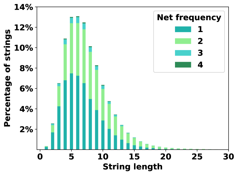
(a) $n=10^{6}$

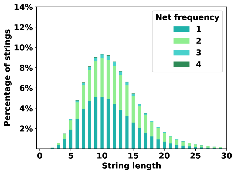
(b) $n=10^{8}$

Figure 3: Net frequency distribution on input texts of two different lengths drawn from NYT corpus. For each string length the column shows the percentage of strings with positive NF; strings of NF larger than $4$ are so rare that they are not visible in this plot.

Algorithms.

As discussed in Section 1, there are no prior efficient algorithms for single-nf. Thus, we came up with two reasonable baselines, CSA and HSA, and compare their performance against our new efficient algorithms, CRL and ASA.

• CRL: presented in Algorithm 1. We implement the algorithm for coloured range listing (CRL) following [30], which uses structures for range minimum query [9].

• ASA: removing the CRL augmentation from Algorithm 1, but keeping all other augmentations, hence the name augmented suffix array (ASA). Specifically, we replace “$\mathit{CRL}_{\mathit{BWT}}(l,r)$” with “$\langle l,r\rangle$” in Line 1 of Algorithm 1.

• CSA: algorithmically the same as ASA, but the data structure used is the compressed suffix array (CSA) [32]. We use the state-of-the-art implementation of CSA from the SDSL library (https://github.com/simongog/sdsl-lite). Specifically, their Huffman-shaped wavelet tree [11, 12] was chosen based on our preliminary experimental results.

• HSA: presented in Algorithm 5. Hash table-augmented suffix array (HSA) is a naive baseline approach that does not use LF, LCP, or CRL, but only augments the suffix array with hash tables to maintain the frequencies of the extensions. These hash tables are later used to determine if an extension is unique or not.

1 // return three hash tables containing the frequencies of the left, right, and bidirectional extensions of $S$, together with the extension characters

2 function extension_frequencies($S$):

3       $\langle l,r\rangle\leftarrow$ the SA interval of $S$;

4       // three hash tables:

5       $L\leftarrow\emptyset,R\leftarrow\emptyset,B\leftarrow\emptyset$;

6       for $i=l,\ldots,r$ do

7             $x\leftarrow T[\mathit{SA}[i]-1]$;  $L[x]\leftarrow L[x]+1$;

8             $y\leftarrow T[\mathit{SA}[i]+|S|]$;  $R[y]\leftarrow R[y]+1$;

9             $B[(x,y)]\leftarrow B[(x,y)]+1$;

10      return $L,R,B$;

Algorithm 4 Subroutine in Algorithm 5

1

Input : $S\leftarrow$ a string

2 // see Algorithm 4

3 $L,R,B\leftarrow\textnormal{{extension\_frequencies}}(S)$;

4 $\mathit{\phi}\leftarrow 0$; // the NF of $S$

5 for $(x,y)\in B$ do

6       // unique left and right extensions

7       if $L[x]=1$ and $R[y]=1$ then

8            $\mathit{\phi}\leftarrow\mathit{\phi}+1$;

9      

return $\mathit{\phi}$

Algorithm 5 single-nf baseline

The asymptotic running times of CRL, ASA, CSA, and HSA are $\text{O}(m+\sigma),\text{O}(m+f),\text{O}(m+f\log\sigma)$, and $\text{O}(m+f\cdot\sigma)$, respectively, where $\sigma$ is the size of the alphabet and the query has length $m$ and frequency $f$.

Comparing CRL against ASA, we expect CRL to be faster for more frequent queries as ASA needs to enumerate the entire SA interval of the query string while CRL does not. ASA is compared against CSA to illustrate the trade-off between query time and space usage: ASA is expected to be faster while CSA is expected to be more space-efficient, and indeed this trade-off is observed in our experiments. We also compare ASA against HSA to demonstrate the speedup provided by the augmentations of LF and LCP.

Results.

The average query time of each algorithm is presented in Table 3. Since the results from the three news datasets exhibit similar behaviours, only the results from NYT are included: henceforth, NYT is the representative for the three news datasets. Overall, our approaches, CRL and ASA, outperform the baseline approaches, HSA and CSA, on both NYT and DNA, but all the algorithms are slower on the DNA data because the query strings are much more frequent. Notably, CRL outperforms the baseline by a factor of up to almost $1000$, across all queries, validating the improvement in the asymptotic cost. Since non-existent and unique queries have zero NF by definition, we next specifically look at the results on repeated queries.

All approaches are slower when the query string is repeated, as further NF computation is required after locating the string in the data structure. For this reason we additionally report results on queries with positive NF. For NYT, similar relative behaviours are observed, but for DNA, all algorithms are significantly faster, likely because strings with positive NF on DNA data are shorter and have much lower frequency. For the same reason of queries being less frequent, ASA is faster than CRL on DNA queries with positive NF because the advantage of CRL over ASA is more apparent when the queries are more frequent.

Table 3: Average single-nf query time (in microseconds) over all the queries, repeated queries ($f\geq 2$), and queries with positive NF ($\mathit{\phi}>0$). The query set from NYT has $2\times 10^{6}$ queries in total, $38.3\%$ repeated, while $1.4\%$ have positive NF. The query set from DNA has $3\times 10^{6}$ queries in total, $51.9\%$ repeated, while $2.5\%$ have positive NF.

Dataset	Algorithm	All	$f\geq 2$	$\mathit{\phi}>0$
NYT	CRL	3.9	7.3	12.6
	ASA	9.4	21.4	39.7
	HSA	695.0	1813.9	3755.4
	CSA	1002.1	2595.7	4884.3
DNA	CRL	6.8	10.1	5.5
	ASA	64.9	122.4	3.3
	HSA	5655.5	10884.9	11.8
	CSA	6348.6	12209.0	10.9

Further results on CRL and ASA.

Previously we have seen that, empirically, the augmentation of CRL accelerates our single-nf algorithm, but is that the case for queries of different frequency and length? We now investigate how query string frequency and length contribute to single-nf query time of CRL and ASA.

For NYT we do not consider strings with frequency greater than 2000, as we observe that these are rare outliers that obscure the overall trend. For each frequency $f\in[0,2000]$ (or length $l\in[5,35]$) and each algorithm $A$, a data point is plotted as the average time taken by $A$ over all the query strings with frequency $f$ (or length $l$). Since there are far more data points in the frequency plot than the length plot, we use a scatter plot for frequency (left of Figure 4) while a line plot for length (right of Figure 4). For frequency, as we anticipated, CRL is faster than ASA on more frequent queries. Empirically, on NYT, the turning point seems to be around 700. Note that the plot for CRL seems more scattered, likely because its time usage does not depend on frequency, but depends on query length. For length, on very short queries, CRL is faster because these queries are highly frequent. Then, generally, query time does not increase as the query strings become longer because they tend to correspondingly become less frequent. This suggests that length is not as significant as frequency in affecting the query time of these approaches.

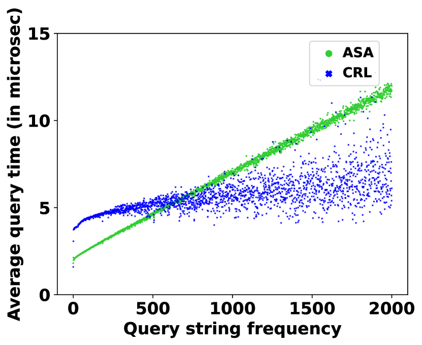
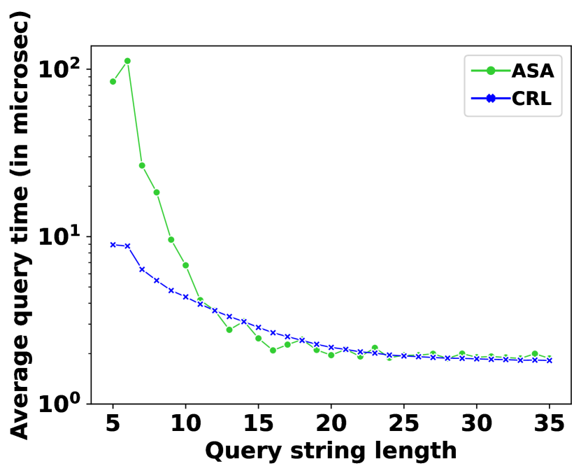
Figure 4: Average single-nf query time (in microseconds) of ASA and CRL against query string frequency (left) and length (right) on the NYT dataset. Note that the $y$-axis on the right is scaled logarithmically.

We similarly examine the effect of frequency and length on ASA and CRL query time using the DNA data. As the query strings are more frequent in DNA than in NYC, we use a higher frequency upper bound of 5000 and the results are presented in Figure 5. The most notable difference between the DNA and NYT is that the former has a much smaller alphabet. Thus, the gap between ASA and CRL becomes more evident for more frequent queries. Additionally, it is notable that the frequency plot for CRL on the DNA dataset appears less scattered compared to the NYT plot, also because of a much smaller alphabet.

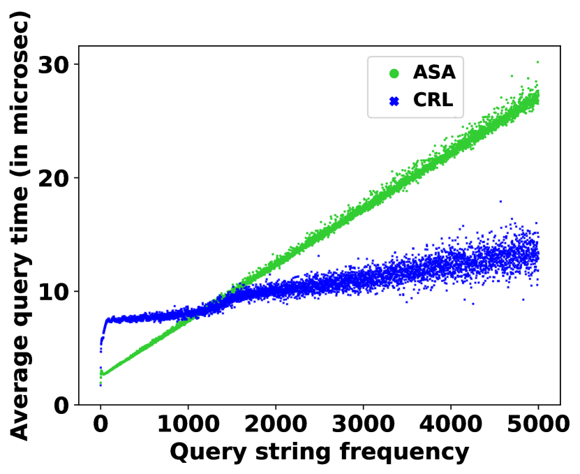
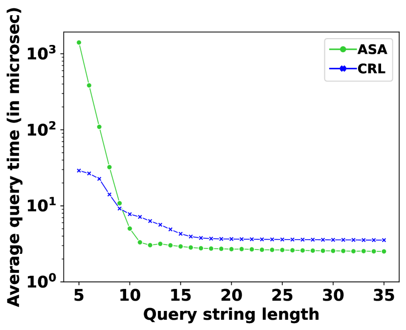
Figure 5: Average single-nf query time (in microseconds) of ASA and CRL against query string frequency (left) and length (right) on the DNA dataset. Note that the $y$-axis on the right is scaled logarithmically.

Remark 5.1.

Although asymptotically CRL is faster than ASA, we have seen that empirically ASA is faster on less frequent queries. This suggests a hybrid algorithm that switches between ASA and CRL depending on the frequency of the query string.

5.2 ALL-NF Experiments

In this section, we present the analyse and empirical results for the two tasks all-nf-report and all-nf-extract. In this setting, each dataset from Table 2 is taken directly an as input text, without having to generate queries. Each reported time is an average of five runs. As seen in Table 4, for all-nf-extract, Algorithm 2 is consistently faster than Algorithm 3 in practice, even though $L\geq N$ (see Definition 4.11). We believe this is because Algorithm 2 is more cache-friendly and does not involve stack operations. Each algorithm is slower for all-nf-report than all-nf-extract, likely due to random-access requirements. For Algorithm 2, although DNA is the largest dataset, the method is faster than on other datasets because there are far fewer strings with positive NF. However, this is not the case for Algorithm 3, because it has to spend much time on other operations, regardless of whether an occurrence is a net occurrence.

Comparing these results to those of the single-nf methods, observe that, for NYT, calculation of NF for each string with $\mathit{\phi}>0$ takes on average 12.6 microseconds, or a total of around 548.5 seconds for the complete set of such strings – which is only possible if the set of these strings is known before the computation begins. Using all-nf, these NF values can be determined in about 39 seconds for extraction and a further 65 seconds to report.

Table 4: Asymptotic cost and average time (in seconds) for all-nf. Build involves building an augmented suffix array including the off-the-shelf suffix array, the LCP array, and the LF mapping of text $T$. See Definition 4.11 for $L$ and $N$. Recall that $N\leq L$ and $L\in\text{O}(n\log\delta)$.

Task	Approach	Cost	Average time
			NYT	APW	XIE	DNA
Build	prior alg.	$\text{O}(n)$	186.7	61.3	39.0	219.6
Extract	Alg. 2	$\text{O}(L)$	38.8	13.6	8.6	6.6
	Alg. 3	$\text{O}(N)$	100.1	33.2	21.9	76.2
Report	Alg. 2	$\text{O}(L+n)$	65.6	20.8	14.3	6.7
	Alg. 3	$\text{O}(n)$	231.6	81.2	52.6	77.4

6 Conclusion and Future Work

Net frequency is a principled method for identifying which strings in a text are likely to be significant or meaningful. However, to our knowledge there has been no prior investigation of how it can be efficiently calculated. We have approached this challenge with fresh theoretical observations of NF’s properties, which greatly simplify the original definition. We then use these observations to underpin our efficient, practical algorithmic solutions, which involve several augmentations to the suffix array, including LF mapping, LCP array, and solutions to the colour range listing problem. Specifically, our approach solves single-nf in $\text{O}(m+\sigma)$ time and all-nf in $\text{O}(n)$ time, where $n$ and $m$ are the length of the input text and a string, respectively, and $\sigma$ is the size of the alphabet. Our experiments on large texts showed that our methods are indeed practical.

We showed that there are at least three net occurrences in a Fibonacci word, $F_{i}$, and verified that these are the only three for each $i$ until reasonably large $i$. Proving there are exactly three is an avenue of future work. We also proved that $\Omega(n)\leq N\leq L\leq\text{O}(n\log\delta)$. Closing this gap remains an open problem. Another open question is determining a lower bound for single-nf. We have focused on static text with exact NF computation in this work. It would be interesting to address dynamic and streaming text and to consider how approximate NF calculations might trade accuracy for time and space usage improvements. Future research could also explore how bidirectional indexes [2, 3, 4, 22] can be adapted for NF computation.

References

- [1] Mohamed Ibrahim Abouelhoda, Stefan Kurtz, and Enno Ohlebusch. Replacing suffix trees with enhanced suffix arrays. Journal of Discrete Algorithms, 2(1):53–86, 2004. doi:10.1016/S1570-8667(03)00065-0.
- [2] Yuma Arakawa, Gonzalo Navarro, and Kunihiko Sadakane. Bi-directional r-indexes. In 33rd Annual Symposium on Combinatorial Pattern Matching, CPM 2022, June 27-29, 2022, Prague, Czech Republic, volume 223 of LIPIcs, pages 11:1–11:14. Schloss Dagstuhl - Leibniz-Zentrum für Informatik, 2022. doi:10.4230/LIPICS.CPM.2022.11.
- [3] Djamal Belazzougui and Fabio Cunial. Smaller fully-functional bidirectional BWT indexes. In String Processing and Information Retrieval - 27th International Symposium, SPIRE 2020, Orlando, FL, USA, October 13-15, 2020, Proceedings, volume 12303 of Lecture Notes in Computer Science, pages 42–59. Springer, 2020. doi:10.1007/978-3-030-59212-7\_4.
- [4] Djamal Belazzougui, Fabio Cunial, Juha Kärkkäinen, and Veli Mäkinen. Versatile succinct representations of the bidirectional Burrows-Wheeler Transform. In Algorithms - ESA 2013 - 21st Annual European Symposium, Sophia Antipolis, France, September 2-4, 2013. Proceedings, volume 8125 of Lecture Notes in Computer Science, pages 133–144. Springer, 2013. doi:10.1007/978-3-642-40450-4\_12.
- [5] Dennis A. Benson, Mark Cavanaugh, Karen Clark, Ilene Karsch-Mizrachi, James Ostell, Kim D. Pruitt, and Eric W. Sayers. Genbank. Nucleic Acids Research, 46(Database-Issue):D41–D47, 2018. doi:10.1093/nar/gkx1094.
- [6] Anders Roy Christiansen, Mikko Berggren Ettienne, Tomasz Kociumaka, Gonzalo Navarro, and Nicola Prezza. Optimal-time dictionary-compressed indexes. ACM Transactions on Algorithms, 17(1):8:1–8:39, 2021. doi:10.1145/3426473.
- [7] Larry J. Cummings, D. Moore, and J. Karhumäki. Borders of Fibonacci strings. Journal of Combinatorial Mathematics and Combinatorial Computing, 20:81–88, 1996.
- [8] Aldo de Luca. A combinatorial property of the Fibonacci words. Information Processing Letters, 12(4):193–195, 1981. doi:10.1016/0020-0190(81)90099-5.
- [9] Johannes Fischer and Volker Heun. Space-efficient preprocessing schemes for range minimum queries on static arrays. SIAM Journal on Computing, 40(2):465–492, 2011. doi:10.1137/090779759.
- [10] Travis Gagie, Juha Kärkkäinen, Gonzalo Navarro, and Simon J. Puglisi. Colored range queries and document retrieval. Theoretical Computer Science, 483:36–50, 2013. doi:10.1016/j.tcs.2012.08.004.
- [11] Simon Gog, Timo Beller, Alistair Moffat, and Matthias Petri. From theory to practice: Plug and play with succinct data structures. In Experimental Algorithms - 13th International Symposium, SEA 2014, Copenhagen, Denmark, June 29 - July 1, 2014. Proceedings, volume 8504 of Lecture Notes in Computer Science, pages 326–337. Springer, 2014. doi:10.1007/978-3-319-07959-2\_28.
- [12] Simon Gog and Enno Ohlebusch. Compressed suffix trees: Efficient computation and storage of LCP-values. ACM Journal of Experimental Algorithmics, 18, 2013. doi:10.1145/2444016.2461327.
- [13] Costas S. Iliopoulos, Dennis W. G. Moore, and William F. Smyth. A characterization of the squares in a Fibonacci string. Theoretical Computer Science, 172(1-2):281–291, 1997. doi:10.1016/S0304-3975(96)00141-7.
- [14] Hiroe Inoue, Yoshiaki Matsuoka, Yuto Nakashima, Shunsuke Inenaga, Hideo Bannai, and Masayuki Takeda. Factorizing strings into repetitions. Theory of Computing Systems, 66(2):484–501, 2022. doi:10.1007/S00224-022-10070-3.
- [15] Juha Kärkkäinen, Dominik Kempa, and Marcin Piatkowski. Tighter bounds for the sum of irreducible LCP values. Theoretical Computer Science, 656:265–278, 2016. doi:10.1016/j.tcs.2015.12.009.
- [16] Juha Kärkkäinen, Giovanni Manzini, and Simon J. Puglisi. Permuted longest-common-prefix array. In Combinatorial Pattern Matching, 20th Annual Symposium, CPM 2009, Lille, France, June 22-24, 2009, Proceedings, volume 5577 of Lecture Notes in Computer Science, pages 181–192. Springer, 2009. doi:10.1007/978-3-642-02441-2\_17.
- [17] Toru Kasai, Gunho Lee, Hiroki Arimura, Setsuo Arikawa, and Kunsoo Park. Linear-time longest-common-prefix computation in suffix arrays and its applications. In Combinatorial Pattern Matching, 12th Annual Symposium, CPM 2001 Jerusalem, Israel, July 1-4, 2001 Proceedings, volume 2089 of Lecture Notes in Computer Science, pages 181–192. Springer, 2001. doi:10.1007/3-540-48194-X\_17.
- [18] Dominik Kempa and Tomasz Kociumaka. Resolution of the Burrows-Wheeler Transform conjecture. In 61st IEEE Annual Symposium on Foundations of Computer Science, FOCS 2020, Durham, NC, USA, November 16-19, 2020, pages 1002–1013. IEEE, 2020. doi:10.1109/FOCS46700.2020.00097.
- [19] Kaisei Kishi, Yuto Nakashima, and Shunsuke Inenaga. Largest repetition factorization of Fibonacci words. In String Processing and Information Retrieval - 30th International Symposium, SPIRE 2023, Pisa, Italy, September 26-28, 2023, Proceedings, volume 14240 of Lecture Notes in Computer Science, pages 284–296. Springer, 2023. doi:10.1007/978-3-031-43980-3\_23.
- [20] Tomasz Kociumaka, Gonzalo Navarro, and Nicola Prezza. Toward a definitive compressibility measure for repetitive sequences. IEEE Transactions on Information Theory, 69(4):2074–2092, 2023. doi:10.1109/TIT.2022.3224382.
- [21] M. Oguzhan Külekci, Jeffrey Scott Vitter, and Bojian Xu. Efficient maximal repeat finding using the Burrows-Wheeler Transform and wavelet tree. IEEE ACM Trans. Comput. Biol. Bioinform., 9(2):421–429, 2012. doi:10.1109/TCBB.2011.127.
- [22] Tak Wah Lam, Ruiqiang Li, Alan Tam, Simon C. K. Wong, Edward Wu, and Siu-Ming Yiu. High throughput short read alignment via bi-directional BWT. In 2009 IEEE International Conference on Bioinformatics and Biomedicine, BIBM 2009, Washington, DC, USA, November 1-4, 2009, Proceedings, pages 31–36. IEEE Computer Society, 2009. doi:10.1109/BIBM.2009.42.
- [23] Yih-Jeng Lin and Ming-Shing Yu. Extracting Chinese frequent strings without dictionary from a Chinese corpus and its applications. Journal of Information Science and Engineering, 17(5):805–824, 2001. URL: https://jise.iis.sinica.edu.tw/JISESearch/pages/View/PaperView.jsf?keyId=86_1308.
- [24] Yih-Jeng Lin and Ming-Shing Yu. The properties and further applications of Chinese frequent strings. International Journal of Computational Linguistics and Chinese Language Processing, 9(1), 2004. URL: http://www.aclclp.org.tw/clclp/v9n1/v9n1a7.pdf.
- [25] M. Lothaire. Combinatorics on words, Second Edition. Cambridge mathematical library. Cambridge University Press, 1997.
- [26] Moritz G. Maaß. Linear bidirectional on-line construction of affix trees. In Combinatorial Pattern Matching, 11th Annual Symposium, CPM 2000, Montreal, Canada, June 21-23, 2000, Proceedings, volume 1848 of Lecture Notes in Computer Science, pages 320–334. Springer, 2000. doi:10.1007/3-540-45123-4\_27.
- [27] Udi Manber and Eugene W. Myers. Suffix arrays: a new method for on-line string searches. SIAM Journal on Computing, 22(5):935–948, 1993. doi:10.1137/0222058.
- [28] Giovanni Manzini. Two space saving tricks for linear time LCP array computation. In Algorithm Theory - SWAT 2004, 9th Scandinavian Workshop on Algorithm Theory, Humlebaek, Denmark, July 8-10, 2004, Proceedings, volume 3111 of Lecture Notes in Computer Science, pages 372–383. Springer, 2004. doi:10.1007/978-3-540-27810-8\_32.
- [29] Burrows Michael and Wheeler David. A block-sorting lossless data compression algorithm. In Digital SRC Research Report, 1994.
- [30] S. Muthukrishnan. Efficient algorithms for document retrieval problems. In Proceedings of the Thirteenth Annual ACM-SIAM Symposium on Discrete Algorithms, January 6-8, 2002, San Francisco, CA, USA, pages 657–666. ACM/SIAM, 2002. URL: http://dl.acm.org/citation.cfm?id=545381.545469.
- [31] Gonzalo Navarro. Indexing highly repetitive string collections, part I: repetitiveness measures. ACM Computing Surveys, 54(2):29:1–29:31, 2022. doi:10.1145/3434399.
- [32] Gonzalo Navarro. Indexing highly repetitive string collections, part II: compressed indexes. ACM Computing Surveys, 54(2):26:1–26:32, 2022. doi:10.1145/3432999.
- [33] Julian Pape-Lange. On extensions of maximal repeats in compressed strings. In 31st Annual Symposium on Combinatorial Pattern Matching, CPM 2020, June 17-19, 2020, Copenhagen, Denmark, volume 161 of LIPIcs, pages 27:1–27:13. Schloss Dagstuhl - Leibniz-Zentrum für Informatik, 2020. doi:10.4230/LIPICS.CPM.2020.27.
- [34] Giuseppe Pirillo. Fibonacci numbers and words. Discrete Mathematics, 173(1-3):197–207, 1997. doi:10.1016/S0012-365X(94)00236-C.
- [35] Mathieu Raffinot. On maximal repeats in strings. Information Processing Letters, 80(3):165–169, 2001. doi:10.1016/S0020-0190(01)00152-1.
- [36] Sofya Raskhodnikova, Dana Ron, Ronitt Rubinfeld, and Adam D. Smith. Sublinear algorithms for approximating string compressibility. Algorithmica, 65(3):685–709, 2013. doi:10.1007/s00453-012-9618-6.
- [37] Ellen M. Voorhees. Overview of TREC 2003. In Proceedings of The Twelfth Text REtrieval Conference, TREC 2003, Gaithersburg, Maryland, USA, November 18-21, 2003, volume 500-255 of NIST Special Publication, pages 1–13. National Institute of Standards and Technology (NIST), 2003. URL: http://trec.nist.gov/pubs/trec12/papers/OVERVIEW.12.pdf.