Neural Semantic Parsing with Extremely Rich Symbolic Meaning Representations

Abstract

Current open-domain neural semantics parsers show impressive performance. However, closer inspection of the symbolic meaning representations they produce reveals significant weaknesses: sometimes they tend to merely copy character sequences from the source text to form symbolic concepts, defaulting to the most frequent word sense based in the training distribution. By leveraging the hierarchical structure of a lexical ontology, we introduce a novel compositional symbolic representation for concepts based on their position in the taxonomical hierarchy. This representation provides richer semantic information and enhances interpretability. We introduce a neural "taxonomical" semantic parser to utilize this new representation system of predicates, and compare it with a standard neural semantic parser trained on the traditional meaning representation format, employing a novel challenge set and evaluation metric for evaluation. Our experimental findings demonstrate that the taxonomical model, trained on much richer and complex meaning representations, is slightly subordinate in performance to the traditional model using the standard metrics for evaluation, but outperforms it when dealing with out-of-vocabulary concepts. This finding is encouraging for research in computational semantics that aims to combine data-driven distributional meanings with knowledge-based symbolic representations.

1 Introduction

The task of formal semantic parsing is to map natural language expressions (words, sentences and texts) to unambiguous interpretable formal meaning representations. The components of these meaning representations can be divided into two parts: the domain-independent logical symbols (such as negation $\lnot$, conjunction $\land$, disjunction $\lor$, equality $=$, and the quantifiers $\exists$, $\forall$), and the non-logical symbols (the concepts and relations between them—the predicates), possibly tailored to a specific domain. It is the latter component that forms the focus of this article, as we see several shortcomings in the way predicates are represented in mainstream computational semantics, since this is usually done by combining a lemma, part-of-speech tag and sense number. This representation of concepts is not only language-specific, but also doesn’t exploit the power of pre-trained language models used in neural approaches, currently the state of the art in semantic parsing Bai, Chen, and Zhang (2022); Martínez Lorenzo, Maru, and Navigli (2022); Wang et al. (2023).

Figure 1: Graphical display of a meaning representation for the sentence John, a keen birdwatcher, was delighted to see a hobby in the style of the Parallel Meaning Bank. Oval nodes represent concepts, boxed nodes introduce contexts, and labeled edges denote thematic roles or semantic relations.

Let us elaborate on this a bit further to make our point clear. Figure 1 shows a meaning representation in the form of a directed acyclic graph, as is common in currently used frameworks in computational semantics Allen, Swift, and de Beaumont (2008); Banarescu et al. (2013); Oepen et al. (2020a); Abzianidze, Bos, and Oepen (2020); Bos (2023). The nodes represent concepts that are symbolized by the lemmas of the content words (nouns, verbs, adjectives, adverbs) that triggered them. As content words are often polysemous, they are usually disambiguated using one of the standard lexical ontologies, including WordNet (Fellbaum, 1998), OntoNotes (Hovy et al., 2006), VerbNet (Bonial et al., 2011) and BabelNet (Navigli and Ponzetto, 2012). This can be done by adding a part-of-speech sign and sense number suffix to the symbol, and is mainstream practice across a wide spectrum of semantic formalisms, such as AMR (Banarescu et al., 2013), BMR (Martínez Lorenzo, Maru, and Navigli, 2022), DRS (Bos et al., 2017), PTG Hajič et al. (2012), EDS Oepen and Lønning (2006). However, the (interrelated) problems that we observe with this approach are the following:

• The same concept can be expressed in various ways (synonyms in the same language, or with different lemma’s in different languages). Yet, they are usually represented with different predicate symbols;

• The predicate symbols possess minimal or no inherent semantic structure. This makes it impossible to determine how they are related to other predicates without access to external knowledge bases;

• The predicate symbols are essentially atomic. Yet, a neural network’s tokenizer will typically break down the symbols into meaningless sequences of characters to reduce the size of its vocabulary.

The first problem can be illustrated with a simple example. Consider the English synonyms car and automobile. In most current approaches, their concepts would be represented with different predicate symbols (e.g., car.n.01 and automobile.n.01, following WordNet), even though they share the same lexical meaning. For non-English lexicalizations for this concept, for instance Italian macchina or French voiture, one could opt to use English-based predicate symbols (as is done by Abzianidze et al. (2017) or use a multi-lingual lexical ontology Tedeschi and Navigli (2022), but these solutions are not language-neutral.

The second problem has risen more to the foreground with the rise of distributional semantics to capture word meanings. While certain predicate symbols exhibit an accidental internal structure that provides additional insight about them (e.g., blackbird.n.01 is a kind of bird.n.01), for most symbols, it is not possible to determine, without external resources, that dog.n.01 is closely related to and compatible with animal.n.01 or puppy.n.01. This is in stark contrast with semantics based on embeddings where meanings are represented by large vectors based on their contextual occurrences in corpora Mikolov, Yih, and Zweig (2013). Some attempts have already been made to close the gap between semantic networks and semantic spaces Rothe and Schütze (2015); Saedi et al. (2018); Scarlini, Pasini, and Navigli (2020); Lees et al. (2020).

The third problem is perhaps more of a theoretical issue, with the desire to use a clean and sound methodology for composing meanings. From an engineering point of view, what happens under the hood of a semantic parser isn’t that important as long as it produces satisfactory accuracy scores. However, a clear disadvantage is that predicted concepts are not guaranteed to exist in the external knowledge base (e.g., WordNet).

These three issues were not particularly pressing in the past or considered problematic, perhaps mainly because word sense disambiguation was seen as a separate task in the sequential symbolic pipeline of traditional semantic parsing. However, the advent of neural methods in semantic processing has magnified these concerns. Neural networks, due to their statistical nature, are confined to their training data distribution, and are therefore struggling in understanding and generating out-of-distribution concepts Groschwitz et al. (2023). Additionally, neural networks tend to find typographical correspondences between the input words and output concepts Edman (2024), thereby copying from the input which, we argue, artificially inflates parsing performance scores. Nevertheless, we believe that pre-trained language models possess the capability to comprehend the semantics of unseen words and concepts within context, but the current representations used in semantic parsing form an obstacle to exploit it.

Let us illustrate this issue with the following scenario. Consider a neural semantic parser trained on a corpus that pairs English sentences with meanings that encode concepts in the standard symbolic format based on a lemma and a sense number. We give this parser the sentence in Figure 1 about birdwatcher John who spotted a hobby, a rare type of falcon. Assume that the word hobby is not in the training data at all. It is very likely that this kind of parser would associate the word hobby with the incorrect concept hobby.n.01, the "spare-time activity" sense, because it learned how to lemmatize from other examples and the suffix "n.01" appears to be the most frequent noun sense. By chance, the parser could produce the correct concept hobby.n.03 (the bird sense), maybe because the suffix "n.03" is often associated with lemmas that end in "by". In our view, we don’t want to develop semantic parsers that make a wild guess for unknown concepts. Instead, we would like to develop semantic parsers that make an educated guess: perhaps it could come up with a concept that it has seen during training, e.g., bird.n.01 or even falcon.n.01 that appears in a similar context as the sentence it tries to parse. Our aim is to combine pre-trained language models with symbolic meaning representations. One possibility to achieve this is to combine semantic parsing with word sense disambiguation based on sense embeddings but this approach requires extensive resources and is not language neutral. Instead, we present a way to develop such a semantic parser by making use of taxonomical encodings.

2 Taxonomical Encodings

In this article we radically deviate from the view of representing non-logical symbols based on lemmas, part-of-speech tags and sense numbers. Instead we introduce a way to encode concepts and relations with internally structured blocks of meaning based on external lexical ontologies or taxonomies. These predicate symbols are not directly interpretable for human beings as they do not correspond to units of language. For instance, the taxonomical encodings for cat and dog share a common prefix that tells us that both are of the category mammal. The encodings for adjectives like good and bad will be very similar, with the only difference indicating that they are antonyms. The idea, llustrated in Figure 2, draws inspiration from research in image classification Mukherjee, Garg, and Roy (2021); Bertinetto et al. (2020).

Figure 2: Simple illustration of a taxonomical encoding. Each box denotes a concept within a typical ontological ISA-hierarchy. The longer the encoding, the more specific its concepts is.

Our research questions are the following. First of all, how can we take existing lexical ontologies as a starting point to encode symbols for concepts (nouns, verbs, adjectives, adverbs) in a compositional way? Secondly, are current neural models actually capable of learning these abstract symbols that have no direct connection with any surface form of language, without reducing parsing performance too much? And finally, do taxonomical encodings of concepts give the semantic parser the ability to make sense of out-of-distribution concepts by assigning a meaning that is compatible with or close to the ground truth, rather than producing a symbol based on the lemma of the word and hoping for the best. In other words, can the parser make an educated guess based on distributional meaning rather than on superficial features when it encounters word meanings that it has never seen before, taking advantage of pre-trained language models?

Our work’s primary contribution lies in presenting a taxonomy-based approach to meaning representation, which is very distinct from prior methods. Accordingly, we connect symbolic and neural techniques in a semantic parsing system. It is symbolic because the semantic parser generates interpretable and transparent meaning representations. It is neural because it harnesses the power of distributional meaning models and neural networks to enhance robustness in unexpected circumstances. A direct consequence of our new approach to semantic parsing is that current evaluation methods, that are based on graph matching, are not sufficient for our purposes, as comparing concepts will be beyond simple string matching and needs to be based and implemented using semantic rather than syntactic similarity. Hence, to assess the capabilities to deal with out-of-vocabulary concepts, we have developed a new challenge test and new semantic evaluation tools. Our experiments reveal that our new representation-based parser performs comparably to the original representation in standard tests but excels in predicting unknown concepts on challenge sets.

3 Background and Related Work

3.1 Semantic Parsing

Early approaches to semantic parsing were mostly based on rule-based systems with compositional semantics defined on top of a syntactic structure obtained by a parser Woods (1973); Hendrix et al. (1977); Templeton and Burger (1983). The development of syntactic treebanks contributed to the creation of robust statistical syntactic parsers, thereby facilitating semantic parsing with broad coverage Bos et al. (2004). The emergence of neural methodologies and the availability of extensive semantically annotated datasets Bos et al. (2017); Banarescu et al. (2013); Abzianidze et al. (2017) marked a shift in semantic parsing techniques, diminishing the emphasis on syntactic analysis van Noord and Bos (2017). The introduction of pre-trained language models within the sequence-to-sequence framework led to further enhancements in parsing accuracy Samuel and Straka (2020); Shou and Lin (2021); Lee et al. (2021, 2022); Bai, Chen, and Zhang (2022); Martínez Lorenzo, Maru, and Navigli (2022); Wang et al. (2023).

Various meaning representations have been the target for semantic parsing Oepen et al. (2020b). Dominating in the field is semantic parsing for Abstract Meaning Representation, AMR, facilitated by the large supply of annotated data and the simplicity of its meaning structures. In this work we focus on DRS, a richer meaning representation, a semantic formalism that drew substantial interest in computational semantics Bos et al. (2004); Evang and Bos (2016); van Noord et al. (2018b); van Noord, Toral, and Bos (2019); Evang (2019); Liu, Cohen, and Lapata (2019); van Noord, Toral, and Bos (2020); Wang et al. (2021); Poelman, van Noord, and Bos (2022); Wang et al. (2023).

3.2 Evaluating Semantic Parsing

A common way of evaluating semantic parsing is to compare parser output with a gold standard using graph overlap Allen, Swift, and de Beaumont (2008); Cai and Knight (2013); van Noord et al. (2018a). A well-known implementation is Smatch, Semantic Match, that measures the structural similarity by mapping graphs into triples and determining the maximum amount of triples that are shared by two semantic graphs, computed by taking the harmonic mean of precision and recall of matching triples Cai and Knight (2013). Smatch is mostly used to assess AMR parsing, but not exclusively, and Poelman, van Noord, and Bos (2022) adopt it for DRS parsing. The original Smatch implements matching of semantic material without further nuances, so several variations and extensions of Smatch have been proposed and developed to enhance semantic evaluation.

Cai and Lam (2019) argue that more weight should be given to triples that form the core of the meaning expressed by a semantic graph. They propose a variant of Smatch that based root-distance by reducing the significance of triple matches that are further away from the root of the graph Cai and Lam (2019). In the meaning representations of our choice, DRS, there is no designated root, so we cannot adopt this variant of Smatch straightaway. Although we think the idea of giving more importance to triples that form the core of the meaning expressed by a text is interesting, we believe more research is required to establish what exactly constitutes this and we therefore will consider this outside the scope of this article.

Opitz, Parcalabescu, and Frank (2020) argue that the "hard" matching of Smatch is not always justified and propose S²Match, Soft Similarity Match, by implementing a graded semantic match of concepts with the help of a distance function that computes a number between $0$ and $1$. The distance function can be anything that fulfills its purpose. Opitz, Parcalabescu, and Frank (2020) showcase their idea using GloVe embeddings to get a similarity score between lemmas. Wein and Schneider (2022) propose LaBSE embeddings Feng et al. (2022) to compute the similarity between two concepts in different languages for cross-lingual comparison of meaning representations. However, these choices of distance functions ignore scenarios where different concepts are expressed by the same lemma. We embrace the use of S²Match in our work but will replace the distance function by an operation that measures the ontological distance between two concepts or relations.

3.3 WordNet

We make heavy use of the lexical ontology WordNet, a handcrafted electronic dictionary Fellbaum (1998). In WordNet, words are organized around synsets, i.e., sets of words that have similar meanings. A synset consists of one or more words; an ambiguous word (a word with more than one sense) is placed into several synsets, one for each distinct meaning. Synsets are connected to each other by several semantic relations (see below). Each synset has a unique identifier, a 9-digit number based on the byte offset in the WordNet database, where the first number identifies the part of speech.

The original WordNet was designed for English Fellbaum (1998). Subsequent efforts have been undertaken to establish WordNets for various languages and to develop multilingual lexical resources Navigli and Ponzetto (2012); Vossen (1998); Bond and Foster (2013), or to include WordNet into a formal ontology Gangemi et al. (2003) and to integrate it with Wikipedia Suchanek, Kasneci, and Weikum (2008); Speer, Chin, and Havasi (2017).

Only parts of speech of content words are included in WordNet: nouns (n), verbs (v), adjectives (a), and adverbs (r). There are several ways to refer to a specific synset: by using the unique identifier, or more commonly, by a combination of lemma, part of speech, and sense number of one of its members. For instance, the English noun hobby is placed into three synsets in Princeton’s WordNet for English: the first sense, hobby.n.01, is glossed as "an auxiliary activity", and two of its other synset members are pursuit.n.03 and avocation.n.01; hobby.n.02 denotes the sense of plaything for children, and hobby.n.03 refers to the bird of prey with the scientific name Falco subbuteo.

The power of WordNet manifests itself by the relations between synsets that it offers. The hypernym and hyponym relations connect generic with specific synsets. For instance, the direct hypernym of hobby.n.03 is falcon.n.01. Synsets that share the same hypernym are called co-hyponyms. For example, hobby.n.03 and peregrine.n.01 are co-hyponyms, as they are both falcons. Verbs are similarly organised in WordNet, but the term troponym is used instead of hyponym to indicate a more fine-grained sense of a verb. For instance, falcon.v.01 is a troponym of hunt.v.01. Some verbs are related to other verbs via the entailment relation, e.g., oversleep.v.01 entails sleep.v.01, and some verbs have derivationally related forms corresponding to nouns, e.g., hunt.v.01 is related to hunt.n.08.

Adjectives and adverbs are quite differently inserted into WordNet than nouns and verbs are. Adjectives are arranged by falling into one of the categories of head and satellite, the former playing a more pivotal role, and the latter a specialisation of a certain adjective. For some adjectives, there exists the antonym relation between synsets of head adjectives, indicating opposite meanings. For instance, good.a.01 and bad.a.01 are antonyms, with satellites cracking.a.01, superb.a.02, among others, for the former, and awful.a.01 and terrible.a.02 (among many others) for the latter. Some adjectives are connected to attribute nouns, e.g., fast.a.01 has the attribute synset speed.n.02. Adjectives are also connected to their derivationally related forms of verbs and nouns. Some adverbs are connected to adjective by the pertainym relation, e.g., quickly.r.01 is a pertainym of quick.a.01. However, there are several adverbs that have no connection with other synsets in WordNet.

The structure of WordNet triggered various proposals to calculate some kind of similarity score between two concepts: the Wu-Palmer similarity Wu and Palmer (1994), the Resnik similarity Resnik (1995) and the Leacock & Chodorow similarity Leacock and Chodorow (1998). In our work, we employ the Wu-Palmer method to compute the conceptual distance between synsets, because it is the simplest of the three and suffices for our purposes. It calculates the distance of two synsets by computing the ratio of the depth of their least common subsumer (LCS, e.g., the first hypernym they share) and the depths of the two synsets, as shown in Equation 1.

$$\textrm{WPS}=2*\frac{depth(\textrm{LCS}(s_{1},s_{2}))}{depth(s_{1})+depth(s_{2})}$$ (1)

For instance, the WPS of the first and third (semantically unrelated) senses of the noun hobby is low: WPS(hobby.n.01, hobby.n.03)=0.087, whereas the similarity between hobby (the bird) and falcon is high: WPS(falcon.n.01, hobby.n.03)=0.963. Note that the similarity metrics mentioned are grounded in WordNet’s taxonomy and typically are most appropriate for noun comparisons, and less so for other parts of speech. In Section 4, we delve into the distinct taxonomies of verbs, adjectives, and adverbs in WordNet. These structural differences lead to inaccuracies in measuring concept similarity for non-noun categories using the existing WordNet taxonomy. To address this issue, we calculate the similarity using the taxonomy encodings described in Section 4 instead of using original WordNet taxonomy. It should also be highlighted that cosine similarity is commonly employed for assessing the similarity between two vectors, which could also be applied to our encodings discussed in Section 2. However, this method is less preferred because it would assign equal weight to every element within the vector, thereby overlooking the inherent hierarchical structure of encodings.

3.4 Non-logical Symbols, Concepts, and Word Senses

Symbolic meaning representations consists of the logical and non-logical parts. The non-logical symbols, the predicates and relations, define the concepts in the domain of interest. Here we assume an open-domain approach where nouns, verbs, adjectives and adverbs are mapped to predicates taken from an ontology, proper names and numbers are mapped to literals, and prepositions and implicit arguments are mapped to an inventory of roles and relations.

In NLP, distinct formats for non-logical symbols have been adopted, ranging from words, lemmas, a combination of a lemma and a sense number, to entries in a lexical ontology. In AMR, predicate symbols are typically derived from PropBank framesets Kingsbury and Palmer (2002), formatted either as lemma-sense and are restricted to verbs. Nouns in AMR are simply represented by their lemmas, and not subject to further disambiguation. In DRS in the style of the Parallel Meaning Bank (Abzianidze et al., 2017, PMB) predicates for noun, verbs, adjectives and adverbs follow the corresponding WordNet synsets and adheres strictly to the lemma-pos-sense format (Figure 1).

Hence, one important subtask of semantic parsing is Word Sense Disambiguation (WSD), the process of identifying the appropriate meaning of a word within its context. Traditionally, this is approached as a classification task with the goal of selecting the correct sense from a set of predefined sense inventories Bevilacqua et al. (2021). In contrast, the task of concept prediction in semantic parsing is treating WSD as a generative task. Here, semantic parsers are expected to generate the correct word sense without given the inventories of senses. This presents a significant challenge, as it is considered currently “impossible” to accurately generate word senses without external knowledge sources, particularly when the word senses have not been encountered in the training data Groschwitz et al. (2023).

The treatment of the WSD task by neural networks can essentially be viewed as a computation involving the comparison of sense embeddings. This involves computing the embedding of a word within its context and contrasting this with the neural encoding listed in the sense inventory. In the case of semantic parsing, the sense number system acts as an instrument for sense prediction. However, numbering senses is fairly arbitrary, only constrained by the tendency that senses encountered frequently in corpora get assigned a low sense number. Consequently, for concepts not encountered in the training data, predicting whether a word corresponds to sense number 3, 4 or 5 holds no distinguishable difference: the best strategy to use for a WSD component would be choosing a low sense number, like 1 or 2. A new representation for concepts presented in Section 4 addresses this issue by refraining from using sense numbers and instead incorporating taxonomical information in concept representation.

Using sense embeddings is perhaps an alternative. Various approaches have been introduced to generate the sense embeddings: AutoExtend Rothe and Schütze (2015) derives synset and lexeme embeddings from word embeddings, and SensEmBERT Scarlini, Pasini, and Navigli (2020) employs the word2vec algorithm Mikolov et al. (2013) for training on a sense-annotated corpus. There are two potential approaches to incorporate sense embeddings, but each has its own limitations. The first method involves replacing the model and tokenizer’s embeddings with pre-trained sense embeddings to provide the model with a basic understanding of WordNet senses. However, this method faces two drawbacks: the pre-trained sense embeddings are independently trained, leading to compatibility issues, such as mismatched dimensions (300 dimensions for AutoExtend and 2048 for SensEmbERT, which do not align with the 768 dimensions of the T5-base model and 1024 dimensions of the T5-large). The second problem is that this method would drastically increase the size of tokenizer’s dictionary, considering that WordNet has more than 100,000 senses.

Another approach is to use the embeddings in the same way as our proposed encodings. However, the substantial dimensionality of embeddings, represented by floating-point numbers, means that explicitly merging them into representations of meaning would significantly increase the representation length. Although compressing their dimensions and transforming the numbers into integers could serve as a potential solution, this approach would result in a huge information loss. Additionally, the interpretability of the resulted embeddings is substantially lower compared to our proposed symbolic encodings, and is relying on annotated corpora available only for a few languages.

3.5 Discourse Representation Structures

In order to run our experiments we need a reasonably-sized annotated corpus of sentences and their meaning representations. Several such annotated corpora are available for AMR, Abstract Meaning Representation Banarescu et al. (2013), and the majority of current semantic parsing methods are developed using AMR datatset. However, for our purposes, we are not able to make use of these linguistic resources because only part of the non-logical symbols (predicates) are disambiguated in AMR, as we outlined in the previous section).

Instead, we will work with a variant of Discourse Representation Structure (DRS), the meaning representation proposed in Discourse Representation Theory Kamp and Reyle (1993). The Parallel Meaning Bank (PMB) offers a large corpus of sentences paired with DRSs with concepts represented by WordNet synsets and a neo-Davidsonian event semantics with VerbNet-inspired thematic roles.

x1 x2 x3 s1 s2 e1 x4
male.n.02(x1)  Name(x1, "John")
keen.a.01(s1)  AttributeOf(s1,x3)
person.n.01(x2)  x2=x1  Role(x2,x3)
birdwatcher.n.01(x3)
delighted.a.01(s2)  Experiencer(s2,x1)  Topic(s2,e1)
see.v.01(e1)  Experiencer(e1,x1)  Stimulus(e1,x4)
hobby.n.03(x4)

male.n.02 Name "John"

keen.a.01 AttributeOf +2

person.n.01 EQU -2 Role +1

birdwatcher.n.01

delighted.a.01 Experiencer -3 Topic +1

see.v.01 Experiencer -1 Stimulus +1

hobby.n.03

Figure 3: Discourse Representation Structure for a sentence shown in box format (left) and sequence notation (right). The corresponding graph for this DRS is shown in Figure 1.

The formal language of DRS consists of discourse referents, and DRS conditions. DRS conditions are predicates applied to discourse referents, relations between discourse referents or literals, or comparison statements (i.e., equality, approximately, temporal precedence, see Appendix). DRSs are recursive data structures; complex DRSs can be constructed to express negation, conjunction, and discourse relations.

An example DRS in box format, the equivalent for the meaning representation graph in Figure 1, is shown on the left in Figure 3. However, in our experiments in Section 6, we will use neither of these formats when training our semantic parsing models. Instead, we will use the sequence notation for DRS where variables are replaced by De Bruijnian indices Bos (2023). The sequence notation is a convenient way for training neural semantic parsers that are based on seq2seq architectures, because there are variables names and a minimal amount of punctuation symbols. Our running example in sequence notation is shown on the right in Figure 3.

4 Encoding Concepts and Relations

There are four parts of speech in WordNet, all with a different ontological organisation. Therefore, we describe for each category how we compute its taxonomical encodings. These encodings will be our new way to represent concepts in a formal meaning representation and used to improve semantic parsing. We use Princeton WordNet version 3.0 Fellbaum (1998), compatible with the Parallel Meaning Bank.

4.1 Nouns

For the encoding of nouns we will make use of the WordNet hyponym-hypernym relation between synsets. Each noun synset has one or more hypernyms, except entity.n.01, which therefore represents the most general synset. For noun synsets with more than one synset (i.e., indicating multiple inheritance) we consider just one of the possible hypernyms.

This procedure maps all the noun synsets to one large isa-hierarchy with the top node entity.n.01. Given a synset within this obtained hierarchy, we give each direct hyponym-hypernym edge a label (a single ASCII character, excluding the zero "0"), ensuring that the labels for each co-hyponyms are all distinct. Once we have done this for each edge, we can read off a unique sequence of labels for each synset. The maximum length of this sequence is the maximum depth of hyponym-hypernym links in WordNet. We pad encodings with trailing zeroes in order to give each synset encoding the same length The number of different labels that we need corresponds to the maximum of co-hyponyms for a synset in WordNet.

Table 1 gives a snapshot of how this labeling works. The resulting taxonomical code gives us a symbolic representation that groups similar concepts (i.e., synsets) together based on their internal structure. The more labels that they share from left-to-right in the encoding, the more they have in common. The more zeroes an encoding has, the more general its synsets is. To distinguish noun synsets from other parts of speech, we attach the prefix "n" to the encoding.

Table 1: Snapshot of generated taxonomy encodings for a group of related noun synsets. Synonyms receive the same encodings, hyponyms get encodings that are more specific (less zeroes).

WordNet synset member	WordNet ID	Taxonomical encoding
entity.n.01	100001740	n$1000000000000000000000$
food.n.01	100021265	n$1233100000000000000000$
beverage.n.01	107881800	n$1233110000000000000000$
drink.n.03	107881800	n$1233110000000000000000$
alcoholic_drink.n.01	107884567	n$1233111000000000000000$
alcohol.n.01	107884567	n$1233111000000000000000$
brew.n.01	107886572	n$1233111100000000000000$
beer.n.01	107886849	n$1233111110000000000000$
booze.n.01	107901587	n$1233111200000000000000$
brandy.n.01	107903208	n$1233111210000000000000$

4.2 Verbs

For verb synsets we follow essentially the same procedure as for nouns presented in tne previous section making use of the troponym and entailment relations available in WordNet. However, the hierarchy of verbs is much flatter than that of nouns, resulting in too many top nodes (synsets without hypernym). For verb synsets without a hypernym, we create edges to noun synset to which they are derivationally related, as shown in Table 2. For noun synsets inserted in this way, we expand the hierarchy as we did for nouns. To distinguish verb concepts from noun-derived concepts, we attach the prefix "v" to it.

Table 2: Snapshot of generated taxonomy encodings that link verb synsets to a noun synset.

WordNet synset member	WordNet Id	Taxonomical encoding
change_of_integrity.n.01	100376063	n$1111211500000000000000$
separation.n.09	100383606	n$1111211510000000000000$
removal.n.01	100391599	n$1111211511000000000000$
get_rid_of.v.01	202224055	v$1111211511100000000000$
throw_away.v.01	202222318	v$1111211511110000000000$
abandon.v.01	202228031	v$1111211511111000000000$
dump.v.02	202224945	v$1111211511120000000000$

4.3 Adjectives and Adverbs

For adjective synsets we create a hierarchical link between satellites and their heads. The head adjectives will be related to noun synsets using derivationally related verb or noun synsets or attribute nouns. To distinguish the adjective encodings, we attach the prefix "a" to it. Antonyms receive the same encodings but are decorated with a positive or negative suffix. WordNet doesn’t provide information whether an antonym is positive or negative, so we use a simple heuristic to check the prefix of the adjective’s lemma (im-, non-, un-), see van Son Chantal, van Miltenburg, and Morante (2016); Blanco and Moldovan (2010). Adverbs are linked to adjectives via the pertainym relation and receive the same encoding but with the prefix "r".

Table 3: Snapshot of generated taxonomy encodings that link adjective and adverb synsets to a noun synset. Encodings for adjectives and adverbs have an additional suffix encoding polarity.

WordNet synset member	WordNet Id	Taxonomical encoding
speed.n.02	105058140	n$1133931000000000000000$
fast.a.01	300976508	a$1133931100000000000000$$+$
fast.r.01	400086000	r$1133931100000000000000$$+$
lazy.a.01	300981304	a$1133931121000000000000$$-$
slow.a.01	300980527	a$1133931120000000000000$$-$
slowly.r.01	400161630	r$1133931120000000000000$$-$
quick.a.01	300979366	a$1133931130000000000000$$+$
haste.n.01	105060189	n$1133931300000000000000$
abruptness.n.03	105060476	n$1133931310000000000000$
sudden.a.01	301143279	a$1133931311000000000000$ $|$
all_of_a_sudden.r.02	400061677	r$1133931311000000000000$ $|$
suddenly.r.01	400061677	r$1133931311000000000000$ $|$

4.4 Roles, Operators and Discourse Relations

The meaning representations that we employ follow a neo-Davidsonian way of representing events Parsons (1990), where events are related to their participants by a close set of thematic roles, i.e., Agent, Theme, Patient, Result, and so on. The inventory of roles is an extension of the hierarchical set proposed in VerbNet Bonial et al. (2011), extended with roles used in the Parallel Meaning Bank. The elaboration of the complete taxonomy of these roles is meticulously outlined in Appendix 8. There are also roles to connect non-event entities, for instance those appearing in genitive constructions or noun compounds. Some thematic roles are paired with their inverse roles, for instance, Sub and SubOf. To clearly distinguish between these roles, we employ distinct prefixes: ’t’ denotes a thematic role, whereas ’i’ signifies an inverse role.

We also convert each Discourse Relation and operator into distinct mathematical symbols, as shown in Appendix 9. In contrast to roles, these two logical components lack a taxonomy structure, therefore their encoding is straightforward, involving a direct mapping to single-byte symbols.

4.5 Semantic Graph with Taxonomical Encodings

Following the encoding process, we can transform the semantic graph into a graph encoded with the WordNet Identifier and WordNet taxonomical encoding, as illustrated in the graphs in Appendix 7. The sequential representations of meanings, which are used for training in Section 6, are illustrated in Table 4.

Table 4: First-order Logic representation and the three sequential meaning representations (Lemma-Pos-Sense, WordNet-Identifier and Taxonomical-encodings) for "John doesn’t laugh."

FOL	$\exists$x(male.n.02(x) $\land$ Name(x,"John") $\land$ $\exists$t(time.n.08(t) $\land$ t=now
	$\lnot\exists$e(laugh.v.01(e) $\land$ Agent(e,x) $\land$ Time(e,t)))
LPS	male.n.02 Name "John" time.n.08 EQU now
	NEGATION <1 laugh.v.01 Agent –2 Time –1
WID	109624168 500000018 "John" 115135822 = now
	$\neg$ <1 200031820 500000004 –2 500000003 –1
TAX	n1222211O00000000000000 t12000 "John" n1133222000000000000000 = now
	$\neg$ <1 v9200000000000000000000 t22100 –2 t21000 –1

5 Developing Taxonomy-based Semantic Tools

Several new tools are required to work with the taxonomical encoding of concepts that we proposed in the previous section. First of all, we need to revise the existing way of measuring semantic parsing performance. We will do so by replacing the well-known Smatch metric with one that takes concept similarity into account. Second, we need a new challenge set that measures parsing performance on out-of-distribution concepts. Finally, we need to add an interpretation component to the semantic parser that maps taxonomical encodings back to human-readable concepts.

5.1 Soft Semantic Matching using the WordNet Taxonomy

We adopt Opitz, Parcalabescu, and Frank (2020)’s S²Match framework (see Section 3.2) but replace its distance function to incorporate taxonomical encodings. Recall that Smatch converts a semantic graph into node-edge-node triples and computes a score based on the maximum number of matching triples. In standard Smatch, two triples get a matching score of 1 if and only if there is a perfect match between the two nodes and the edge. S²Match extends this approach by introducing a soft matching between instance triples, where a distance function based GloVe embedding similarity returns a score between 0 and 1. We modify Smatch and S²Match with respect to three issues:

1. We replace the distance function based on word embeddings by the Wu-Palmer Score (see Section 3.3);

2. We not only allow soft matching based on the Wu-Palmer Score for instance triples, but also for role triples;

3. In the implementation of Smatch, triples featuring TOP were discarded since DRS, unlike AMR, does not contain roots.

In the rest of this article we refer to these alterations of Smatch and S²Match as Hard Smatch and Soft Smatch, respectively. Note that the Wu-Palmer distance based on the standard WordNet taxonomy struggles with accurately measuring the distance for verbs, adjectives, and adverbs because these parts of speech have less hierarchical structure and are sometimes unconnected. To overcome this limitation, we measure the distance with the generated encodings discussed in Section 4, enabling a more precise computation of Wu-Palmer similarity.

5.2 Creating a Challenge Set for Out-of-Distribution Concepts

One of our research objectives is to make a model that is able to come up with a reasonable interpretation of a concept that it has never encountered during training. The Parallel Meaning Bank offers training, development, and test sets, all featuring similar distributions (Figure 4). The PMB data indicates that concepts are frequently with the first word sense. This is not very surprising, because WordNet tends to list the most used senses first for each word.

Figure 4: Distribution of word senses in the different data splits of the Parallel Meaning Bank. Note that except sense "01", sense "02" is prominent because every person name incorporates either the female.n.02 or male.n.02 and "08" also stands out because every meaning for a tensed clause includes the time.n.08 concept.

This poses the following problem to meet our research objective. Say we give the model for semantic parsing a sentence with an unknown word (a word that the model hasn’t seen during training). The model will likely transform it into a WordNet concept with sense number $1$, based on the statistics seen on training. Hence, the chance that the model got it correct is very high. But does such a model demonstrate some kind of semantic understanding? Not really—it just produced a pattern that it has seen many, many times during training.

In this case, we need to evaluate capability of dealing with rare or unseen word senses. We do this by creating a challenge test set consisting of more than a hundred English sentences and their gold standard meaning representations, where each sentence contains one or more words (nouns, verbs, or adjectives) that are not part of the training and development set, or are present in the training set with a different sense. To ensure an insightful evaluation, we make certain that the corresponding meaning for these unknown concepts do not correspond to the first sense. As a source of inspiration we use the glosses and example sentences found in WordNet for a particular word sense, and add enough context to disambiguate the meaning of the word. For instance, in "the moon is waxing", we have the third sense for the verb, resulting in the concept wax.v.03, not seen in training (although wax.v.01 could be part of the training data).

After gathering $129$ example sentences containing $103$ unknown nouns, $37$ unknown verbs and $27$ adjectives/adverbs, we conduct manual annotations on these samples to guarantee their gold-standard quality. For sentences that are deficient in contextual details, we supplement additional context to enhance their significance. In Table 9 in Section 6, we showcase some examples along with the predictions of different parsers.

5.3 Desiging a Taxonomy-based Semantic Parsing Architecture

Modern semantic parsing predominantly employs sequence-to-sequence models. In our approach, we retain the sequence-to-sequence architecture but adapt the output to represent a linearized graph of semantic representation encoded with taxonomical encodings. This output representation needs to undergo a process of interpretation (Figure 5). This interpretation is implemented by mapping the taxonomical encodings into concepts and relations of our human-readable dictionary. This dictionary consists of WordNet and the ontology of other symbols including the semantic roles. In other words, what the mapper does is translating each encoding into a traditional format found in the standard meaning representations.

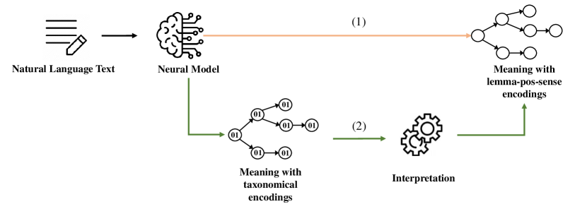
Figure 5: The pipelines for semantic parsing in comparison. Route (1) shows a neural semantic parsing system based on traditional concepts representations. Route (2) illustrates the taxonomy-based parsing system where a mapper interprets the produced symbols.

Let $\cal{M}$ be a dictionary that maps taxonomical encodings to unambiguous predicate symbols, much like as shown in Tables 1–4. Let $T_{n}$ denote a taxonomical sequence meaning representation of length $n$, where $T_{n}=(t_{1},t_{2},\ldots,t_{n})$. Then the interpretation function $\mathcal{I}$ is defined as follows:

$$\mathcal{I}(T_{n})=(I(t_{1}),I(t_{2}),\ldots,I(t_{m}),\ldots,I(t_{n}))$$ (2)

$$I(t_{m})=\left\{\begin{array}[]{ll}\mathcal{M}(t_{m}),&\text{if }t_{m}\in\text{tax-format}\text{ and }t_{m}\in\mathcal{M}\\ \mathcal{M}(C(t_{m})),&\text{if }t_{m}\in\text{tax-format}\text{ and }t_{m}\notin\mathcal{M}\\ t_{m},&\text{otherwise}\end{array}\right.$$ (6)

The function $\mathcal{I}$ denotes the symbolic interpretation process, encapsulating the overall mapping. The function $I$ operates on individual elements within the tax code sequence. If an element $t_{m}$ strictly follows the tax code format and is listed in the dictionary, it is directly mapped to the corresponding lemma-pos-sense, role, operator or discourse relation format. If it is not part of the dictionary but a valid taxonomical encoding it undergoes computation by the function $C$. This is a traversal function that sifts through all tax codes in the mapping to identify the encoding most similar to the input according to the Wu-Palmer similarity. Elements that are not encoded are regarded as literals and left unchanged.

In our parsing system, taxonomical encodings serve as an intermediate representation, not as the final output. The interpretation component in the pipeline (Figure 5) generates a meaning graph that is readable for humans, encoded with lemma-pos-sense information and the usual labels for roles, operators, and discourse relations format (Table 10). The advantages of taxonomical encodings will be revealed in the following experiment sections.

6 Experiments and Results

We will compare three different representation methods for conceptual predicates: the standard one based on lemma, part of speech and sense number (LPS, henceforth), one based on rather arbitrary WordNet identifiers (WID), and one based on our novel taxonomical encodings (TAX). The data that we use to run our experiments is drawn from the Parallel Meaning Bank. For evaluation we employ both the standard test set to assess the overall semantic parsing accuracy (for English and German) as well as the challenge set dedicated to measure the ability to interpret concepts not part of the training data (for English only).

6.1 Data

For our experiments, we selected the gold-standard English and German data from the Parallel Meaning Bank as detailed in Table 5. English data is divided into training, development, and test sets following an 8:1:1 split ratio, and German data follows 4:3:3 split ratio to make the development and test sufficiently large for evaluation purposes.

Table 5: Data statistics for two languages in the PMB 5.0.0. Words and Chars represents the average number of words and characters in one sample.

	Train			Development			Test
	Samples	Words	Chars	Samples	Words	Chars	Samples	Words	Chars
English	9,057	5.6	24.5	1,132	5.4	24.9	1,132	5.2	25.1
German	1,206	5.1	25.7	900	4.8	25.7	900	4.9	25.6

6.2 Experimental Settings

In our experiments, we utilized the most frequently used seq2seq architecture, specifically leveraging the transformer-based T5 Raffel et al. (2019) and BART Lewis et al. (2020), two pre-trained transformer-based architectures. Specifically, we fine-tuned their multilingual variants (because we include both English and German): mT5 Xue et al. (2021), byT5 Xue et al. (2022) and mBART Liu et al. (2020). mT5 builds upon the T5 model with pre-training on multi-languages corpus. byT5 enhances the multilingual approach through byte-level processing, making it especially effective at handling languages with limited data resources. Meanwhile, mBART also leverages multilingual corpus for its pre-training phase and adopts a denoising autoencoder strategy. A noteworthy distinction between these models lies in their tokenization approaches: mT5 and mBART utilize sub-word tokenization, while byT5 employs byte-level tokenization. In our task, whether employing the lemma-pos-sense notation, WordNet identifiers, or taxonomical encodings, each presents a format distinct from those languages which encounter in the pre-training corpus. This divergence challenges the models’ tokenization strategies and their proficiency in processing new language with limited data.

We set the learning rate to $1e-4$, included a decay rate of $0.1$ and set a patience threshold of $5$ for early stopping. More details are provided in Appendix 11. Given the relatively small size of the German dataset for fine-tuning (1,206 instances for training), we initially train the models on the English data for $3$ epochs before fine-tuning them with the German data. Each experiment is ran three times to calculate the average and standard deviation, which are detailed in the results tables.

6.3 Results on Semantic Parsing

The results for semantic parsing for each of the three different meaning representations are presented in Table 6 (English) and Table 7 (German). We show the standard (hard) Smatch score (HSm) for exact semantic matching and the soft Smatch score (SSm) for approximate semantic matching. We also include the rate of ill-formed output (IFR), as the seq2seq architectures that we employ do not guarantee well-formed graph meaning representations (any output that is ill-formed is assigned a score of $0$).

Table 6: Semantic parsing results (Hard Smatch, Soft Smatch, Ill-formed Rate) for English using three different models: Lemma-Pos-Sense, WordNet-IDs, and taxonomical encodings.

	LPS			WID			TAX
	HSm	SSm	IFR	HSm	SSm	IFR	HSm	SSm	IFR
mT5	75.4 $\pm 2.6$	78.5 $\pm 2.1$	8.7 $\pm 0.8$	79.3 $\pm 2.5$	82.7 $\pm 2.3$	3.9 $\pm 0.9$	74.0 $\pm 3.2$	82.3 $\pm 3.8$	3.4 $\pm 0.9$
byT5	87.5 $\pm 1.8$	89.1 $\pm 2.3$	4.7 $\pm 0.4$	84.7 $\pm 1.1$	86.9 $\pm 1.0$	2.7 $\pm 0.5$	85.3 $\pm 2.3$	90.3 $\pm 2.5$	2.0 $\pm 0.6$
mBART	81.1 $\pm 1.2$	83.7 $\pm 2.2$	5.0 $\pm 0.7$	83.3 $\pm 0.9$	83.9 $\pm 0.5$	3.0 $\pm 0.6$	81.4 $\pm 3.6$	88.4 $\pm 3.6$	2.1 $\pm 0.4$

The standard Smatch scores are a little bit below earlier reported F-scores on PMB data (Hard Smatch score $94.7$ English and $92.0$ for German, as reported by Wang et al. (2023)), but they are decent considering that we only train on the gold data part and we don’t employ pre-training. Besides, our research objective is not to reach the highest performance, but rather compare performance of differently structured predicate symbols in meaning representations. The results for German (Table 7) are lower than those for English. We think this is caused by two factors: there is, compared to English, less typographical correspondence between the input words and output meanings, and there is less training data available for German. Nonetheless, the results for German are in line with those for English.

Let us next compare the performance of the three architectures. Despite the fact that all models are based on the seq2seq and encoder-decoder framework, they exhibit non-consistent performance on these three representations. This is due to the difference in their pre-training objectives and corpora, activation functions, parameter initialization and other aspects (we kindly refer the reader to the original papers of these models, see Section 6.2). For instance, in English, mT5 and mBART, when trained using the WID representation, show superior Hard Smatch score compared to both LPS and TAX. Conversely, LPS get higher Hard Smatch score than WID and TAX using byT5.

Table 7: Semantic parsing results (Hard Smatch, Soft Smatch, Ill-formed Rate) for German using three different models: Lemma-Pos-Sense, WordNet-IDs, and taxonomical encodings.

	LPS			WID			TAX
	HSm	SSm	IFR	HSm	SSm	IFR	HSm	SSm	IFR
mT5	67.5 $\pm 2.2$	71.4 $\pm 2.4$	15.2 $\pm 1.7$	60.8 $\pm 2.3$	66.4 $\pm 2.1$	13.0 $\pm 1.3$	66.3 $\pm 2.4$	75.4 $\pm 2.5$	6.3 $\pm 1.5$
byT5	80.1 $\pm 1.1$	83.2 $\pm 1.2$	5.4 $\pm 0.6$	78.6 $\pm 1.0$	83.0 $\pm 1.3$	5.8 $\pm 0.8$	79.4 $\pm 1.2$	85.6 $\pm 1.3$	3.0 $\pm 0.7$
mBART	74.8 $\pm 2.3$	78.7 $\pm 2.5$	6.5 $\pm 0.6$	62.5 $\pm 2.4$	69.2 $\pm 2.3$	4.1 $\pm 0.7$	76.3 $\pm 2.1$	84.8 $\pm 1.1$	1.7 $\pm 0.7$

The byT5 model achieved the highest Smatch scores among for all settings and both languages. We believe that the tokenization strategy of byT5 is the main reason for its good performance. This is in line with the findings of van Noord, Toral, and Bos (2020), who suggest that DRS parsing benefits from the character-level tokenization. Giving a concrete example, mT5’s sub-word tokenizer segments $hobby.n.03$, $101612476$, and $n1222212113423100000000$ into disjointed chunks like $[hobby,.,n,.03]$, $[10,1612,476]$, and $[n,1222,2121,1342,31,00000000]$, respectively. In contrast, byT5’s byte-level tokenizer processes the same inputs into $[h,o,b,b,y,.,n,.,0,3]$, $[1,0,1,6,1,2,4,7,6]$, and $[n,1,2,2,2,1,2,1,1,3,4,2,3,1,0,0,0,0,0,0,0,0]$, offering a more meaningful and robust segmentation. This distinction is particularly crucial for taxonomical encodings, where each character represents a specific layer within the taxonomy.

In the rest of this discussion we will focus on byT5 given its superior performance. Let us delve into the comparison of the three semantic representations, based on ByT5’s performance. Based on the Hard Smatch scores, LPS emerged as the top performer, achieving scores of $80.1$ for English and $78.3$ for German. WID and TAX perform similarly: both are slightly lower than LPS. This result aligns with our expectations considering the LPS model’s tendency to copy the lemma while typically assigning a sense number of $01$ to each concept. As illustrated in Section 5.2, it is common for concepts to carry the sense number $01$, and LPS clearly benefits from this.

However, the situation changes when we turn to look at the results of approximate semantic matching, where the TAX-parser demonstrates better performance ($90.3$ for English and $85.6$ for German). The Soft Smatch score improved by a minimum of $5$ points over Hard Smatch, reaching a peak increase of $8.7$ for English and $9.1$ for German. Conversely, while the Soft Smatch scores for both LPS and WID saw a modest rise, both the magnitude of their increases and final Soft Smatch scores fell short when compared to the TAX-parser. In this case, the larger increase demonstrates that TAX is doing something interesting that LPS and WID are not capable of. In Section 6.4 we will perform a deeper analysis of this behaviour.

Considering the ill-formed rate we can observe that there are two main causes for ill-formed outputs. One is that the index points to a non-existent concept, and the other is that the generated graph is cyclic. We found that both the WID-parser and TAX-parser have significantly reduced the frequency of index-related prediction errors, which in case reduce the IFR for both English and German. These errors typically stem from the model’s limited understanding of the generated graph structure. The low IFR can be seen as the evidence that proposed uniform representation using encodings enhances the seq2seq model’s comprehension of semantic graph structures.

6.4 Results on Unknown Concept Identification

Although the overall results for semantic parsing already favor our newly proposed taxonomical encodings (TAX), we also want to show that TAX is making fewer absurd predictions than its alternatives, LPS and WID. In Section 5.2 we presented a challenge test set for semantic parsing that contains out-of-distribution concepts. There are two ways to look at the results of the three different approaches on this stress test: globally, using Smatch scores; or locally, looking in detail on how the three approaches react on unknown concepts. The global results in terms of Hard Smatch and Soft Smatch metrics remain in line with the results of the standard tests of the previous section: for ByT5, the LPS-parser scores the highest Hard Smatch ($77.0$) while the TAX-parser scores the highest Soft Smatch ($80.1$).

Table 8: Results on unknown concept identification for nouns, verbs, and adjectives, comparing meaning representations based on the standard lemma-pos-sense notation (LPS), WordNet identifiers (WID), with taxonomical encodings (TAX).

Category	Number	LPS	WID	TAX
noun	103	0.395	0.483	0.510
verb	37	0.328	0.357	0.393
adjective & adverb	27	0.503	0.373	0.374

For a more fine-grained analysis we looked at how the three approaches dealt with the unknown concepts. For each example sentence in the challenge test set we identified the unknown concepts and paired them with the prediction of the corresponding concepts in the output meaning representation. This was done via an automatic alignment of concepts followed by human verification and correction when needed. Then we applied the Wu-Palmer similarity to each concept pair (gold vs. predicted). The results of identifying these unknown concepts are presented in Table 8.

As Table 8 shows, none of the three approaches performs very well. Recall that achieving a perfect score on this task is highly unlikely — only by chance a parser might pick the correct word sense. Hence, all three parsers are expected to make mistakes, but there are important differences in the severity of these mistakes (Table 9).

The taxonomical encodings (TAX) show the best performance for unknown noun and verb concepts. The standard notation following the lemma-pos-sense (LPS) convention yields mediocre results because the parser will in most cases default to the most frequent (first or second) sense following the sense distribution in the training data (Table 9). The WID (WordNet IDs) parser performs surprisingly well, so the identifiers exhibit some systematic grouping that we are not aware of. Unknown verb concepts seem harder to predict, perhaps because they show less hierarchical structure in WordNet than nouns.

The LPS model makes the best predictions for adjectives and adverbs. This can probably be attributed to two factors. Firstly, there is even less hierarchical structure in WordNet for adjectives and adverbs, and the Wu-Palmer measure that we use for similarity is not optimal for adjectives and adverbs, as it doesn’t take polarity into account in a principled way. Secondly, the training set includes only a modest number of adjectives (2,665) and adverbs (609), limiting the model to effectively learn the taxonomical information inside the encodings. In contrast, with adequate data for nouns (33,675) and verbs (8,097), the model significantly benefits from taxonomical information.

Table 9: Some instances of the challenge set with words with out-of-vocabulary concepts in bold face, and the concepts predicted by the lemma-pos-sense parser (LPS) and the taxonomical encoding parser (TAX). In brackets the Wu-Palmer similarity score between gold and prediction.

Input Text	Gold	LPS prediction	TAX prediction
… went birdwatching. She saw … a hobby.	n.03	hobby.n.01 (0.09)	big_cat.n.01 (0.67)
The thrush’s song filled the forest with …	n.03	thrush.n.01 (0.17)	pigeon.n.01 (0.79)
The soldier was shot in the calf.	n.02	calf.n.01 (0.20)	arm.n.01 (0.57)
He wore a sling for his broken arm.	n.02	sling.n.01 (0.20)	suit.n.01 (0.67)
Jennifer cooked the bass in a large steamer.	n.02	steamer.n.01 (0.20)	microwave.n.02 (0.48)
… mayor proposed extensive cuts in the city …	n.19	cut.n.01 (0.24)	removal.n.01 (0.73)
Tiger Woods aced the 16th hole.	v.03	ace.v.02 (0.25)	penetrate.v.01 (0.18)
… musician was playing a … fugue …	n.03	fugue.n.01 (0.25)	harp.n.01 (0.20)
He shuffled the cards.	v.02	shuffle.v.01 (0.25)	rip.v.01 (0.80)
The moon is waxing.	v.03	wax.v.01 (0.25)	wake_up.v.02 (0.76)
The elephant’s trunk is an extended nose.	n.05	trunk.n.02 (0.26)	nose.n.01 (0.91)
The stripper in the club did a strip for us.	n.03	stripper.n.01 (0.27)	sailor.n.01 (0.73)
She dressed the salad.	v.10	dress.v.01 (0.29)	chew.v.01 (0.24)
The woman wore a short black mantle.	n.08	mantle.n.02 (0.36)	kimono.n.01 (0.78)
He has a very dry sense of humor.	a.02	dry.a.01 (0.38)	weak.a.01 (0.20)
The escaped convict took to the hills.	v.27	take.v.09 (0.45)	run.v.01 (0.78)
A tiny wren was hiding in the shrubs.	n.02	wren.n.01 (0.54)	pen.n.05 (0.81)
David was armed with a sling.	n.04	sling.n.02 (0.59)	bow.n.02 (0.67)
Hungarian is a challenging language with …	n.02	hungarian.n.02 (1.00)	italian.n.02 (0.54)
… was playing a … fugue on the grand.	n.02	grand.n.02 (1.00)	scene.n.01 (0.40)
They played Scrabble in the living room.	n.02	scrabble.n.02 (1.00)	chess.n.02 (0.82)

As Table 9 illustrates, the LPS model is extremely good at transforming word forms to a lemma and a high frequency sense number, but this strategy does not fare well on the challenge set. In fact, it makes severe mistakes, predicting thrush (the infection) instead of thrush (the bird), or Micky Mantle (the baseball player) rather than mantle (the garment). However, there were several cases where the LPS-parser had a "lucky strike", when it picked the second sense for a lemma which happened to be correct. A case in point is Hungarian (the language), where the LPS picked the second sense, perhaps because most languages in WordNet happen to be assigned the second sense (the first sense is usually the inhabitant of a country).

Most interestingly, in analogy with recent approaches to image classification Mukherjee, Garg, and Roy (2021); Bertinetto et al. (2020), the TAX-parser "makes the best mistakes", as it often predicted concepts similar to the unknowns. Table 9 shows some intriguing examples, e.g., microwave (the kitchen appliance sense) instead of steamer (the cooking utensil sense), or arm (human limb) instead of calf (part of a human leg). It makes mistakes, but less drastic than the mistakes made by the LPS-parser, because it will attempt to find a concept that is close in meaning (exploiting the contextual understanding of the pre-trained language model) rather than copying a lemma from the textual input to output meaning, as the LPS-parser seems to be doing.

7 Conclusion and Future Work

We showed that by take an existing lexical ontology, WordNet, we are able to generate hierarchical compositional encodings for predicate symbols for nouns, verbs, adjectives, and adverbs. We complemented these with encodings for semantic roles, relations, and operators. The resulting meaning representations are completely language-neutral (apart from literals, like proper names and numbers, obviously). These extremely rich conceptual representations are still "parseable" for neural models. For English and German, parsing performance is a little bit lower than the standard lemma-pos-sense notation under Hard Smatch (exact semantic matching), which we attribute to the input-output copying capabilities (translation) of the neural models. However, the advantage of taxonomical encodings is evidenced by a higher Soft Smatch score (approximate semantic matching) and a superior identification of out-of-distribution concepts.

We believe that these results are encouraging and a promising way to combine distributional semantics with formal semantics. We hope that the approach presented in this paper is inspirational for future work on neural-symbolic semantic processing. We envision potential both on the neural and the symbolic side.

On the neural side, one interesting direction to explore is incorporating large language models, such as BLOOM, Mistral, and Llama2. Another potential focal point is to investigate modifications of the loss function aimed at enhancing the models’ understanding of taxonomical information in the encodings, where weights are assigned to characters based on their positions. We initiated pilot studies along these ideas but they did not show promising results yet, so we need to investigate why this isn’t working as expected. Also, alternative ways of hierarchical machine learning are worthy of exploration.

On the symbolic side, there is a lot of space to further explore the taxonomical encodings. The current encodings are complex, and perhaps there are ways to reduce the number of layers, or different ways of incorporating verbs and adjectives. Ontology other than WordNet can be explored, different representations of concepts (perhaps pictograms), and better methods for measuring similarity, in particular that of adjectives and adverbs.

Meaning representations in LPS, WID and TAX

We show here the three different types of meaning representations used in our experiments. We do this for the text “John, a keen birdwatcher, was delighted to see a hobby.” in graph format for readability. In the experiments we use the sequence notation.

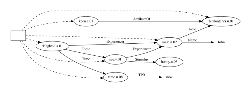
Figure 6: Meaning graph using the lemma-pos-sense (LPS) notation to encode concepts.

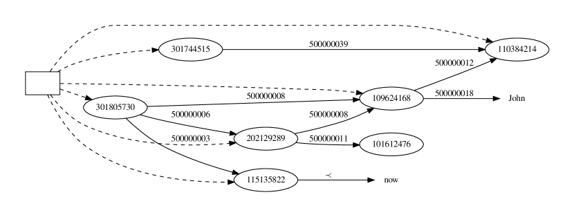
Figure 7: Meaning graph based on unique identifiers (WID). The identifiers for synsets are taken from WordNet. The identifiers for roles are assigned by us.

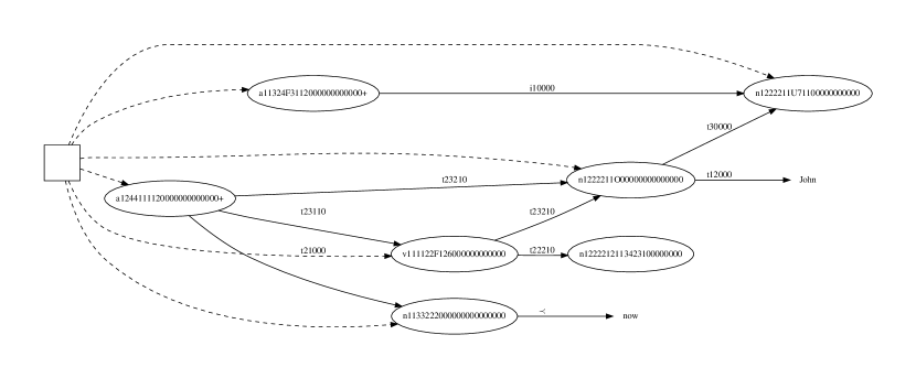
Figure 8: Meaning graph with taxonomical encodings for concepts and roles (TAX).

Taxonomy of Roles used in the Parallel Meaning Bank

Figure 10 shows the hierarchy of roles and relations as used in the Parallel Meaning Bank. This hierarchy is an extension of the one proposed for VerbNet Bonial et al. (2011).

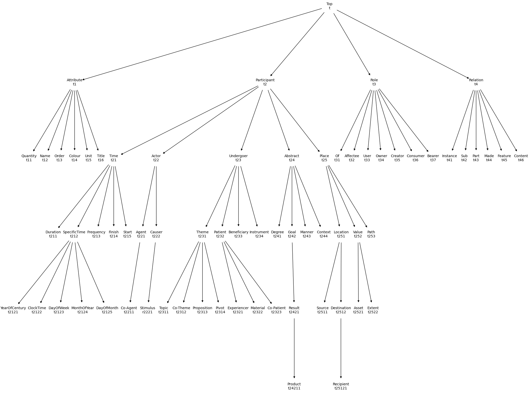
Figure 9: Complete hierarchy of semantic roles used in the semantic parsing experiments. Each role name is shown with the taxonomical encoding.

Taxonomy encodings of Operators and Discourse Relations.

The identifier and character encoding of operators and discourse relations in Table 10 and Table 11.

Table 10: Taxonomy encodings of Operators. Differently from the previous table, the id mentioned here is not the WordNet identifier, but rather one that we have assigned manually.

Operator	Identifier	Char code	Meaning
TPR	700000001	$\prec$	temporal precedes (before)
TSU	700000002	$\succ$	temporal succeeds (after)
TIN	700000003	$\sqsubset$	temporal inclusion
TCT	700000004	$\sqsupset$	temporal contains
TAB	700000005	$\bowtie$	temporal abut
LES	700000006	$<$	less than
LEQ	700000007	$\leq$	less or equal than
TOP	700000008	$\top$	not more than
MOR	700000010	$>$	greater than
EQU	700000011	$=$	equal
ANA	700000012	$\equiv$	anaphoric link
APX	700000013	$\approx$	approximately equal
NEQ	700000014	$\neq$	not equal
SXP	700000015	$\gg$	spatially behind
SXN	700000016	$\ll$	spatially before
SZN	700000017	$\veebar$	spatially under
SZP	700000018	$\curlyvee$	spatially above

Table 11: Taxonomy encodings of Discourse Relations.

Relation	Identifier	Char code
ALTERNATION	600000001	$\lor$
ATTRIBUTION	600000002	$@$
CONDITION	600000003	$\rightarrow$
CONSEQUENCE	600000004	$\Rightarrow$
CONTINUATION	600000005	$\leftrightarrow$
CONTRAST	600000006	$/$
EXPLANATION	600000007	$\infty$
NECESSITY	600000008	$\square$
NEGATION	600000009	$\neg$
POSSIBILITY	600000010	$\diamond$
PRECONDITION	600000011	$\leftarrow$
RESULT	600000012	$\sum$
SOURCE	600000013	$\hookleftarrow$
CONJUNCTION	600000014	$\land$
ELABORATION	600000015	$\supset$
COMMENTARY	600000016	${\dagger}$

Experimental Settings

To facilitate reproduction, we detail the important hyperparameters employed. For the WID and TAX encodings, we adopt a larger patience and decay rate, allowing ample time for convergence. This decision stems from experimental observations indicating that these novel (to the models) representations exhibit a slower convergence rate compared to LPS. We test using hierarchical loss, which give higher weight to the characters on the left within each word, but the initial experiments didn’t show any improvements.

Table 12: Hyperparameters for training different representations.

	Learning Rate	Epoch	Patience	Decay Rate	Optimizer	Loss Function
LPS	1e-4	50	10	0.1	AdamW	Cross Entropy
WID	1e-4	50	15	0.2	AdamW	Cross Entropy
TAX	1e-4	50	15	0.2	AdamW	Cross Entropy

Interpreting Misspellings

In order to assess the ability of models to deal with misspellings we created a test suite of English sentences paired with meaning representations where each sentence contained a commonly misspelled content word, i.e., acceptible, humourous, enterpreneur. The results, shown in Table 13, demonstrate that the traditional lemma-pos-sense notation fails to identify wrongly spelled content words caused by its tendency to copy character sequences from input words to output lemmas.

Table 13: Results on misspelled content words by computing concept identification scores for the three different models: lemma-pos-sense (LPS), WordNet identifiers (WID), and taxonomical encodings (TAX).

Category	Number	LPS	WID	TAX
noun	16	0.105	0.441	0.563
verb	10	0.149	0.648	0.593
adjective	16	0.000	0.415	0.510

Concept Identification Results

Table 14: All instances of the challenge set with words with out-of-vocabulary concepts, and the concepts predicted by the lemma-pos-sense parser (LPS), WordNet identifier (WID) and the taxonomical encoding parser (TAX). In brackets the Wu-Palmer similarity score between gold and prediction.

Gold	LPS	WID	TAX
extract.n.02	extract.n.01 (0.24)	speech.n.01 (0.35)	history.n.02 (0.47)
cruiser.n.03	cruiser.n.01 (0.36)	dancer.n.01 (0.40)	ship.n.01 (0.85)
warbler.n.02	warbler.n.02 (1.00)	fictional_animal.n.01 (0.70)	tower.n.01 (0.45)
rag.n.03	rag.n.01 (0.14)	song.n.01 (0.75)	pot.n.01 (0.20)
harrier.n.03	harrier.n.01 (0.46)	tiger.n.02 (0.67)	shed.n.01 (0.42)
hobby.n.03	hobby.n.01 (0.11)	luggage.n.01 (0.40)	lobby.n.01 (0.40)
stool.n.02	stool.n.01 (0.59)	stadium.n.01 (0.35)	tooth.n.01 (0.30)
eagle.n.02	eagle.n.01 (0.19)	eagle.n.01 (0.19)	eagle.n.01 (0.19)
wallflower.n.03	wallflower.n.01 (0.52)	vegetarian.n.01 (0.70)	comedian.n.01 (0.73)
beetle.n.02	beelte.n.02 (0.00)	bed.n.01 (0.61)	shed.n.01 (0.55)
stake.n.05	stake.n.01 (0.13)	storage_space.n.01 (0.55)	hull.n.06 (0.57)
hungarian.n.02	hungarian.n.02 (1.00)	german.n.02 (0.57)	Sanskrit.n.01 (0.57)
pen.n.02	pen.n.01 (0.60)	pen.n.01 (0.60)	pen.n.01 (0.60)
pen.n.05	pen.n.01 (0.42)	pen.n.01 (0.42)	pen.n.01 (0.42)
gondola.n.02	gondola.n.01 (0.57)	gun.n.01 (0.58)	bottle.n.01 (0.61)
bug.n.03	bug.n.02 (0.19)	coop.n.02 (0.52)	disease.n.01 (0.17)
investigation.n.02	investigation.n.01 (0.33)	practice.n.04 (0.78)	wrongdoing.n.02 (0.82)
thrush.n.03	thrush.n.01 (0.17)	lemur.n.01 (0.71)	hypocrite.n.01 (0.54)
song.n.04	song.n.01 (0.53)	song.n.01 (0.53)	song.n.01 (0.53)
admiral.n.02	admiral.n.01 (0.48)	aunt.n.01 (0.54)	crocodilian_reptile.n.01 (0.57)
flower.n.02	flower.n.01 (0.45)	flower.n.01 (0.45)	flower.n.01 (0.45)
bloom.n.02	bloom.n.01 (0.33)	blood.n.01 (0.33)	blood.n.01 (0.33)
wren.n.02	wren.n.01 (0.57)	grass.n.01 (0.56)	swan.n.01 (0.85)
bed.n.03	ocean_bed.n.01 (0.00)	picture.n.02 (0.47)	beach.n.01 (0.77)
impression.n.04	impression.n.01 (0.38)	tear.n.01 (0.38)	smell.n.01 (0.33)
tripper.n.04	tripper.n.01 (0.40)	tv_set.n.01 (0.61)	elevator.n.01 (0.76)
reel.n.05	reel.n.02 (0.12)	ranch.n.01 (0.17)	bike.n.02 (0.16)
course.n.07	course.n.01 (0.12)	candy.n.01 (0.78)	cup.n.02 (0.27)
mantle.n.08	mantle.n.02 (0.00)	(0.00)	scarf.n.01 (0.82)
joint.n.06	joint.n.01 (0.32)	jet.n.01 (0.23)	joint.n.01 (0.32)
net.n.05	net.n.02 (0.70)	napkin.n.01 (0.55)	net.n.02 (0.70)
rally.n.05	rally.n.02 (0.47)	initiation.n.01 (0.59)	race.n.02 (0.62)
adder.n.03	adder.n.01 (0.38)	back_door.n.03 (0.37)	astronaut.n.01 (0.56)
key.n.04	key.n.03 (0.13)	key.n.01 (0.22)	key.n.01 (0.22)
harrier.n.02	hard_coat.n.01 (0.00)	dog.n.01 (0.91)	joiner.n.01 (0.47)
drive.n.10	drive.n.01 (0.12)	dress.n.01 (0.63)	engine.n.01 (0.80)
fugue.n.03	fugue.n.01 (0.29)	music.n.01 (0.57)	tune.n.01 (0.53)
grand.n.02	grand.n.02 (1.00)	guitar.n.01 (0.78)	restaurant.n.01 (0.57)
application.n.04	application.n.01 (0.30)	comic_book.n.01 (0.17)	application_form.n.01 (0.50)
bag.n.03	bag.n.01 (0.70)	bag.n.01 (0.70)	bag.n.01 (0.70)
cover.n.09	cover.n.01 (0.62)	schoolroom.n.01 (0.57)	mask.n.04 (0.60)
pain.n.04	pain.n.01 (0.20)	pain.n.01 (0.20)	pain.n.01 (0.20)
stripper.n.03	stripper.n.01 (0.29)	wizard.n.02 (0.76)	passenger.n.01 (0.76)
strip.n.06	strip.n.02 (0.21)	trip.n.01 (0.50)	trip.n.01 (0.50)
substance.n.04	substance.n.01 (0.67)	object.n.04 (0.36)	drug.n.01 (0.60)
ray.n.07	ray.n.01 (0.21)	hedgehog.n.02 (0.69)	sand.n.01 (0.25)
increase.n.05	increase.n.01 (0.15)	eye_blink.n.01 (0.21)	rate.n.02 (0.30)
cut.n.19	cut.n.01 (0.27)	art.n.02 (0.60)	trip.n.01 (0.70)
antenna.n.03	antennae.n.01 (0.00)	airline.n.02 (0.20)	skeletal_muscle.n.01 (0.63)
entrance.n.03	entrance.n.02 (0.29)	laugh.n.01 (0.38)	landing.n.04 (0.89)

Gold	LPS	WID	TAX
operation.n.05	operation.n.01 (0.31)	war.n.01 (0.71)	job.n.02 (0.78)
service.n.15	service.n.01 (0.74)	sewing_machine.n.01 (0.18)	service.n.01 (0.74)
whisker.n.02	whisker.n.01 (0.10)	cat.n.01 (0.25)	mouse.n.01 (0.26)
attack.n.07	attack.n.03 (0.21)	cold.n.01 (0.27)	attack.n.07 (1.00)
appearance.n.04	appearance.n.01 (0.43)	negotiation.n.01 (0.38)	athletic_game.n.01 (0.44)
sub.n.02	sub.n.01 (0.29)	stuff.n.02 (0.40)	dagger.n.01 (0.52)
dock.n.03	dock.n.01 (0.44)	dog.n.01 (0.40)	dog.n.01 (0.40)
touch.n.10	touch.n.01 (0.47)	view.n.02 (0.53)	improvement.n.01 (0.44)
weight.n.07	weight.n.01 (0.43)	kilo.n.01 (0.75)	value.n.02 (0.43)
pan.n.03	scale_pan.n.01 (0.00)	sweater.n.01 (0.63)	tumbler.n.02 (0.84)
labor.n.02	labor.n.02 (1.00)	behavior.n.01 (0.82)	job.n.01 (0.82)
unit.n.03	offensive_unit.n.01 (0.00)	college.n.02 (0.75)	school.n.01 (0.75)
period.n.07	period.n.01 (0.33)	time.n.08 (0.33)	time.n.03 (0.35)
top.n.10	top.n.01 (0.47)	toe.n.01 (0.30)	roof.n.01 (0.74)
top.n.09	top.n.02 (0.42)	top.n.02 (0.42)	frontier.n.02 (0.47)
carton.n.02	carton.n.01 (0.13)	calculator.n.02 (0.70)	ax.n.01 (0.61)
trunk.n.05	trunk.n.02 (0.26)	hat.n.01 (0.27)	(0.53)
organ.n.03	organ_onstage.n.01 (0.00)	company.n.01 (0.21)	piano.n.01 (0.82)
cape.n.02	cape.n.02 (1.00)	calculator.n.02 (0.55)	wash.n.07 (0.82)
song.n.05	song.n.01 (0.33)	college.n.02 (0.32)	(0.27)
heat.n.06	heat.n.02 (0.38)	hour.n.01 (0.40)	heat.n.02 (0.38)
mouth.n.04	mouth.n.01 (0.35)	middle.n.01 (0.57)	frontier.n.02 (0.53)
calf.n.02	calf.n.01 (0.42)	calculator.n.02 (0.29)	face.n.01 (0.63)
chemistry.n.03	chemistry.n.01 (0.35)	chemistry.n.01 (0.35)	natural_science.n.01 (0.38)
crown.n.07	crown.n.01 (0.14)	bus_stop.n.01 (0.59)	haunt.n.01 (0.62)
mole.n.03	mole.n.02 (0.22)	bread.n.01 (0.40)	cup.n.01 (0.26)
almond.n.02	almond.n.02 (1.00)	sugar.n.01 (0.24)	entity.n.01 (0.25)
bass.n.04	bass.n.02 (0.12)	pretzel.n.01 (0.63)	sandglass.n.01 (0.29)
steamer.n.02	steamer.n.01 (0.24)	spoon.n.01 (0.52)	pistol.n.01 (0.56)
lock.n.02	lock.n.01 (0.48)	shit.n.01 (0.30)	screw.n.04 (0.48)
ace.n.06	ace.n.08 (0.00)	extraterrestrial.n.01 (0.32)	(0.00)
slide.n.03	slide.n.03 (1.00)	soccer_ball.n.01 (0.20)	sunglasses.n.01 (0.19)
slip.n.11	slip.n.01 (0.11)	sock.n.01 (0.73)	wash.n.07 (0.86)
scrabble.n.02	scrabble.n.02 (1.00)	rugby.n.01 (0.56)	board_game.n.01 (0.86)
decoy.n.02	decoy.n.01 (0.52)	fly.n.01 (0.45)	mosquito.n.01 (0.45)
jay.n.02	jay.n.01 (0.50)	hedgehog.n.02 (0.69)	dolphin.n.02 (0.62)
hole.n.03	hole.n.02 (0.29)	hole.n.02 (0.29)	shore.n.01 (0.33)
hawker.n.02	hawker.n.01 (0.55)	hunter.n.01 (0.96)	guest.n.01 (0.70)
merlin.n.02	merlin.n.01 (0.11)	match.n.01 (0.40)	bat.n.01 (0.71)
rocket.n.03	rocket.n.01 (0.48)	rayon.n.01 (0.53)	spoon.n.01 (0.45)
move.n.05	move.n.01 (0.63)	movie.n.01 (0.59)	assignment.n.05 (0.74)
barrel.n.02	barrel.n.02 (1.00)	basket.n.01 (0.84)	balcony.n.02 (0.67)
function.n.07	function.n.01 (0.38)	baseball_club.n.01 (0.30)	job.n.02 (0.30)
string.n.05	string.n.01 (0.22)	page.n.01 (0.21)	lock.n.01 (0.20)
green.n.06	green.n.02 (0.53)	tomb.n.01 (0.56)	grey.n.05 (0.21)
surge.n.03	surge.n.01 (0.15)	person.n.01 (0.24)	person.n.01 (0.24)
wave.n.06	wave.n.01 (0.21)	quantity.n.01 (0.27)	marker.n.02 (0.22)
sling.n.04	sling.n.02 (0.59)	soccer_ball.n.01 (0.64)	club.n.03 (0.67)
sling.n.05	sling.n.01 (0.20)	sock.n.01 (0.64)	canopy.n.03 (0.67)
china.n.02	china.n.02 (1.00)	continent.n.01 (0.42)	orange_juice.n.01 (0.29)
slug.n.07	slug.n.01 (0.32)	goose.n.01 (0.59)	mosquito.n.01 (0.72)
growth.n.04	growth.n.01 (0.29)	fruit.n.01 (0.24)	flower.n.01 (0.21)
bullfinch.n.02	bullfinch.n.01 (0.57)	metatherian.n.01 (0.74)	chicken.n.02 (0.76)

Table 15: All instances of the challenge set with verbs with out-of-vocabulary concepts.

Gold	LPS	WID	TAX
drive.v.08	drive.v.01 (0.40)	drive.v.01 (0.40)	drive.v.01 (0.40)
house.v.02	house.v.01 (0.00)	(0.00)	(0.00)
run.v.22	run.v.01 (0.15)	run.v.01 (0.15)	run.v.01 (0.15)
release.v.05	release.v.02 (0.27)	step_out.v.01 (0.20)	throw.v.03 (0.19)
serve.v.15	serve.v.07 (0.25)	serve.v.06 (0.50)	give.v.24 (0.50)
run.v.19	run.v.07 (0.24)	work.v.04 (0.24)	pass.v.14 (0.18)
recognize.v.08	recognize.v.01 (0.29)	remind.v.01 (0.17)	draw_up.v.04 (0.14)
describe.v.02	describe.v.01 (0.17)	kvetch.v.01 (0.29)	mislead.v.02 (0.91)
give.v.19	give.v.03 (0.50)	give.v.03 (0.50)	give.v.01 (0.13)
balloon.v.02	balloon.v.02 (1.00)	(0.00)	bathe.v.01 (0.21)
dress.v.10	dress.v.01 (0.29)	overcook.v.01 (0.26)	chew.v.01 (0.24)
ace.v.03	ace.v.02 (0.29)	improve.v.01 (0.18)	penetrate.v.01 (0.18)
poach.v.02	poach.v.01 (0.18)	catch.v.04 (0.18)	pour.v.01 (0.18)
hawk.v.02	hawk.v.01 (0.44)	sign.v.05 (0.29)	meow.v.01 (0.19)
shuffle.v.02	shuffle.v.01 (0.20)	braid.v.03 (0.17)	rip.v.01 (0.80)
bust.v.02	bust.v.01 (0.33)	push.v.01 (0.46)	block.v.01 (0.44)
check.v.19	check.v.01 (0.19)	recognize.v.04 (0.30)	draw_up.v.04 (0.30)
plug.v.04	plug.v.05 (0.25)	bewitch.v.01 (0.33)	search.v.01 (0.35)
ring.v.06	ring.v.01 (0.13)	wave.v.01 (0.18)	write.v.07 (0.42)
bark.v.03	bark.v.04 (0.17)	(0.00)	decapitate.v.01 (0.59)
refresh.v.02	refresh.v.01 (0.40)	leak.v.04 (0.26)	relax.v.01 (0.18)
take.v.27	take.v.09 (0.45)	take.v.09 (0.45)	run.v.01 (0.78)
draw.v.07	draw.v.06 (0.48)	draw.v.06 (0.48)	draw.v.13 (0.92)
order.v.05	order.v.02 (0.71)	order.v.02 (0.71)	dial.v.02 (0.56)
cram.v.03	cram.v.02 (0.15)	demolish.v.03 (0.62)	call.v.05 (0.12)
cram.v.02	cram.v.01 (0.20)	tear.v.01 (0.83)	slice.v.03 (0.80)
challenge.v.02	challenge.v.01 (0.15)	pick_up.v.02 (0.36)	elect.v.01 (0.47)
moderate.v.03	moderate.v.03 (1.00)	clear.v.24 (0.46)	grow.v.02 (0.17)
book.v.03	book.v.02 (0.14)	marry.v.01 (0.55)	allow.v.04 (0.14)
solicit.v.03	solicit.v.02 (0.25)	spy.v.02 (0.40)	sentence.v.01 (0.46)
hobble.v.03	hobble.v.01 (0.25)	brush.v.01 (0.11)	trap.v.04 (0.16)
wax.v.03	wax.v.01 (0.40)	shine.v.02 (0.19)	wake_up.v.02 (0.76)
breach.v.02	breach.v.01 (0.22)	leave.v.05 (0.18)	execute.v.03 (0.67)
swan.v.03	swan.v.01 (0.25)	send.v.01 (0.70)	swim.v.01 (0.45)

Table 16: All instances of the challenge set with adjectives and adverbs with out-of-vocabulary concepts.

Gold	LPS	WID	TAX
calm.a.02	calm.a.01 (0.16)	(0.00)	(0.00)
rare.a.03	rare.a.01 (0.42)	capable.a.05 (0.42)	large.a.01 (0.67)
firmly.r.02	firmly.r.02 (1.00)	all_of_a_sudden.r.01 (0.33)	comfortably.r.02 (0.47)
sturdy.a.03	sturdy.a.02 (0.50)	dirty.a.01 (0.47)	dirty.a.01 (0.47)
short.a.02	short.a.02 (1.00)	short.a.02 (1.00)	short.a.02 (1.00)
muscular.a.02	muscular.a.01 (0.00)	(0.00)	creative.a.01 (0.22)
hard.a.03	(0.00)	(0.00)	jacket.n.01 (0.00)
grand.a.08	grand.a.01 (0.50)	huge.a.01 (0.17)	huge.a.01 (0.17)
extended.a.03	extended.a.01 (0.50)	long.a.02 (0.93)	long.a.01 (0.38)
gently.r.02	gently.r.01 (0.32)	in_public.r.01 (0.47)	(0.50)
dry.a.02	dry.a.01 (0.38)	surprised.a.01 (0.33)	weak.a.01 (0.40)
broken.a.07	broken.a.03 (0.50)	international.a.01 (0.44)	right.a.02 (0.53)
special.a.04	special.a.01 (0.00)	(0.00)	bad.a.01 (0.18)
vicious.a.02	vicious.a.02 (1.00)	fishy.a.02 (0.43)	suspicious.a.01 (0.47)
rugged.a.03	rugged.a.01 (0.59)	dirty.a.01 (0.42)	upper.a.01 (0.16)
rather.r.04	rather.r.02 (0.86)	rather.r.04 (1.00)	rather.r.04 (1.00)
sleazy.a.02	sleazy.a.01 (0.50)	overweight.a.01 (0.53)	greasy.a.02 (0.42)
immature.a.05	immature.a.01 (0.50)	tense.a.01 (0.20)	impenetrable.a.01 (0.57)
plumy.a.03	(0.00)	(0.00)	(0.00)
fairly.r.03	fairly.r.02 (0.50)	quickly.r.02 (0.50)	seriously.r.01 (0.50)
unfledged.a.02	unfledged.a.01 (0.50)	nuts.a.01 (0.17)	wounded.a.01 (0.22)
furious.a.02	furious.a.02 (1.00)	angry.a.01 (0.96)	scared.a.01 (0.45)
uncontrollable.a.03	uncontrollable.a.01 (0.50)	dirty.a.01 (0.27)	unemployed.a.01 (0.52)
smart.a.05	smart.a.01 (0.35)	long.a.01 (0.62)	slow.a.03 (0.33)
horny.a.02	horny.a.01 (0.50)	wild.a.02 (0.17)	ridiculous.a.02 (0.17)
kafkaesque.a.02	(0.00)	(0.00)	armed.a.01 (0.20)
vivid.a.03	vivid.a.02 (0.50)	tired_of.a.01 (0.20)	excruciating.a.01 (0.42)

References

- Abzianidze et al. (2017) Abzianidze, Lasha, Johannes Bjerva, Kilian Evang, Hessel Haagsma, Rik van Noord, Pierre Ludmann, Duc-Duy Nguyen, and Johan Bos. 2017. The Parallel Meaning Bank: Towards a multilingual corpus of translations annotated with compositional meaning representations. In Proceedings of the 15th Conference of the European Chapter of the Association for Computational Linguistics: Volume 2, Short Papers, pages 242–247, Association for Computational Linguistics, Valencia, Spain.
- Abzianidze, Bos, and Oepen (2020) Abzianidze, Lasha, Johan Bos, and Stephan Oepen. 2020. Drs at mrp 2020: Dressing up discourse representation structures as graphs. In Proceedings of the CoNNL 2020 Shared Task: Cross-Framework Meaning Representation Parsing, pages 23–32.
- Allen, Swift, and de Beaumont (2008) Allen, James F., Mary Swift, and Will de Beaumont. 2008. Deep semantic analysis of text. In Semantics in Text Processing. STEP 2008 Conference Proceedings, pages 343–354, College Publications.
- Bai, Chen, and Zhang (2022) Bai, Xuefeng, Yulong Chen, and Yue Zhang. 2022. Graph pre-training for AMR parsing and generation. In Proceedings of the 60th Annual Meeting of the Association for Computational Linguistics (Volume 1: Long Papers), pages 6001–6015, Association for Computational Linguistics, Dublin, Ireland.
- Banarescu et al. (2013) Banarescu, Laura, Claire Bonial, Shu Cai, Madalina Georgescu, Kira Griffitt, Ulf Hermjakob, Kevin Knight, Philipp Koehn, Martha Palmer, and Nathan Schneider. 2013. Abstract Meaning Representation for sembanking. In Proceedings of the 7th Linguistic Annotation Workshop and Interoperability with Discourse, pages 178–186, Association for Computational Linguistics, Sofia, Bulgaria.
- Bertinetto et al. (2020) Bertinetto, L., R. Mueller, K. Tertikas, S. Samangooei, and N.A. Lord. 2020. Making better mistakes: Leveraging class hierarchies with deep networks. In 2020 IEEE/CVF Conference on Computer Vision and Pattern Recognition (CVPR), pages 12503–12512, IEEE Computer Society, Los Alamitos, CA, USA.
- Bevilacqua et al. (2021) Bevilacqua, Michele, Tommaso Pasini, Alessandro Raganato, and Roberto Navigli. 2021. Recent trends in word sense disambiguation: A survey. In Proceedings of the Thirtieth International Joint Conference on Artificial Intelligence, IJCAI-21, pages 4330–4338, International Joint Conferences on Artificial Intelligence Organization. Survey Track.
- Blanco and Moldovan (2010) Blanco, Eduardo and Dan Moldovan. 2010. Automatic discovery of manner relations and its applications. In Proceedings of the 2010 Conference on Empirical Methods in Natural Language Processing, pages 315–324, Association for Computational Linguistics, Cambridge, MA.
- Bond and Foster (2013) Bond, Francis and Ryan Foster. 2013. Linking and extending an open multilingual wordnet. In Proceedings of the 51st Annual Meeting of the Association for Computational Linguistics (Volume 1: Long Papers), pages 1352–1362.
- Bonial et al. (2011) Bonial, C., W. Corvey, M. Palmer, V.V. Petukhova, and H.C. Bunt. 2011. A hierarchical unification of lirics and verbnet semantic roles. In Proceedings IEEE-ICSC 2011 Workshop on Semantic Annotation for Computational Linguistic Resources, pages 1–7, Stanford University.
- Bos (2023) Bos, Johan. 2023. The sequence notation: Catching complex meanings in simple graphs. In Proceedings of the 15th International Conference on Computational Semantics (IWCS 2023), pages 1–14, Nancy, France.
- Bos et al. (2017) Bos, Johan, Valerio Basile, Kilian Evang, Noortje Venhuizen, and Johannes Bjerva. 2017. The groningen meaning bank. In Nancy Ide and James Pustejovsky, editors, Handbook of Linguistic Annotation, volume 2. Springer, pages 463–496.
- Bos et al. (2004) Bos, Johan, Stephen Clark, Mark Steedman, James R. Curran, and Julia Hockenmaier. 2004. Wide-coverage semantic representations from a CCG parser. In COLING 2004: Proceedings of the 20th International Conference on Computational Linguistics, pages 1240–1246, COLING, Geneva, Switzerland.
- Cai and Lam (2019) Cai, Deng and Wai Lam. 2019. Core semantic first: A top-down approach for AMR parsing. In Proceedings of the 2019 Conference on Empirical Methods in Natural Language Processing and the 9th International Joint Conference on Natural Language Processing (EMNLP-IJCNLP), pages 3799–3809, Association for Computational Linguistics, Hong Kong, China.
- Cai and Knight (2013) Cai, Shu and Kevin Knight. 2013. Smatch: an evaluation metric for semantic feature structures. In Proceedings of the 51st Annual Meeting of the Association for Computational Linguistics (Volume 2: Short Papers), pages 748–752, Association for Computational Linguistics, Sofia, Bulgaria.
- Edman (2024) Edman, Lukas. 2024. The Little Data That Could: Making the Most of Low-Resource Natural Language Processing. Ph.D. thesis, University of Groningen.
- Evang (2019) Evang, Kilian. 2019. Transition-based DRS parsing using stack-LSTMs. In Proceedings of the IWCS Shared Task on Semantic Parsing, Association for Computational Linguistics, Gothenburg, Sweden.
- Evang and Bos (2016) Evang, Kilian and Johan Bos. 2016. Cross-lingual learning of an open-domain semantic parser. In Proceedings of COLING 2016, the 26th International Conference on Computational Linguistics: Technical Papers, pages 579–588, The COLING 2016 Organizing Committee, Osaka, Japan.
- Fellbaum (1998) Fellbaum, Christiane, editor. 1998. WordNet: An Electronic Lexical Database. Language, Speech, and Communication. MIT Press, Cambridge, MA.
- Feng et al. (2022) Feng, Fangxiaoyu, Yinfei Yang, Daniel Cer, Naveen Arivazhagan, and Wei Wang. 2022. Language-agnostic BERT sentence embedding. In Proceedings of the 60th Annual Meeting of the Association for Computational Linguistics (Volume 1: Long Papers), pages 878–891, Association for Computational Linguistics, Dublin, Ireland.
- Gangemi et al. (2003) Gangemi, Aldo, Nicola Guarino, Claudio Masolo, and Alessandro Oltramari. 2003. Sweetening wordnet with dolce. AI Magazine, 24(3):13–24.
- Groschwitz et al. (2023) Groschwitz, Jonas, Shay Cohen, Lucia Donatelli, and Meaghan Fowlie. 2023. AMR parsing is far from solved: GrAPES, the granular AMR parsing evaluation suite. In Proceedings of the 2023 Conference on Empirical Methods in Natural Language Processing, pages 10728–10752, Association for Computational Linguistics, Singapore.
- Hajič et al. (2012) Hajič, Jan, Eva Hajičová, Jarmila Panevová, Petr Sgall, Ondřej Bojar, Silvie Cinková, Eva Fučíková, Marie Mikulová, Petr Pajas, Jan Popelka, Jiří Semecký, Jana Šindlerová, Jan Štěpánek, Josef Toman, Zdeňka Urešová, and Zdeněk Žabokrtský. 2012. Announcing Prague Czech-English Dependency Treebank 2.0. In Proceedings of the Eighth International Conference on Language Resources and Evaluation (LREC’12), pages 3153–3160, European Language Resources Association (ELRA), Istanbul, Turkey.
- Hendrix et al. (1977) Hendrix, Gary G., Earl D. Sacerdoti, Daniel Sagalowicz, and Jonathan Slocum. 1977. Developing a natural language interface to complex data. In TODS.
- Hovy et al. (2006) Hovy, Eduard, Mitchell Marcus, Martha Palmer, Lance Ramshaw, and Ralph Weischedel. 2006. OntoNotes: The 90% solution. In Proceedings of the Human Language Technology Conference of the NAACL, Companion Volume: Short Papers, pages 57–60, Association for Computational Linguistics, New York City, USA.
- Kamp and Reyle (1993) Kamp, H. and U. Reyle. 1993. From Discourse to Logic: Introduction to Modeltheoretic Semantics of Natural Language, Formal Logic and Discourse Representation Theory. Number pt. 2 in Developments in Cardiovascular Medicine. Kluwer Academic.
- Kingsbury and Palmer (2002) Kingsbury, Paul and Martha Palmer. 2002. From TreeBank to PropBank. In Proceedings of the Third International Conference on Language Resources and Evaluation (LREC’02), European Language Resources Association (ELRA), Las Palmas, Canary Islands - Spain.
- Leacock and Chodorow (1998) Leacock, Claudia and Martin Chodorow. 1998. Combining local context and wordnet similarity for word sense identification.
- Lee et al. (2022) Lee, Young-Suk, Ramón Astudillo, Hoang Thanh Lam, Tahira Naseem, Radu Florian, and Salim Roukos. 2022. Maximum Bayes Smatch ensemble distillation for AMR parsing. In Proceedings of the 2022 Conference of the North American Chapter of the Association for Computational Linguistics: Human Language Technologies, pages 5379–5392, Association for Computational Linguistics, Seattle, United States.
- Lee et al. (2021) Lee, Young-Suk, Ramón Fernández Astudillo, Thanh Hoang, Tahira Naseem, Radu Florian, and Salim Roukos. 2021. Maximum bayes smatch ensemble distillation for amr parsing. In North American Chapter of the Association for Computational Linguistics.
- Lees et al. (2020) Lees, Alyssa, Chris Welty, Shubin Zhao, Jacek Korycki, and Sara Mc Carthy. 2020. Embedding semantic taxonomies. In Proceedings of the 28th International Conference on Computational Linguistics, pages 1279–1291, International Committee on Computational Linguistics, Barcelona, Spain (Online).
- Lewis et al. (2020) Lewis, Mike, Yinhan Liu, Naman Goyal, Marjan Ghazvininejad, Abdelrahman Mohamed, Omer Levy, Veselin Stoyanov, and Luke Zettlemoyer. 2020. BART: Denoising sequence-to-sequence pre-training for natural language generation, translation, and comprehension. In Proceedings of the 58th Annual Meeting of the Association for Computational Linguistics, pages 7871–7880, Association for Computational Linguistics, Online.
- Liu, Cohen, and Lapata (2019) Liu, Jiangming, Shay B. Cohen, and Mirella Lapata. 2019. Discourse representation structure parsing with recurrent neural networks and the transformer model. In Proceedings of the IWCS Shared Task on Semantic Parsing, Association for Computational Linguistics, Gothenburg, Sweden.
- Liu et al. (2020) Liu, Yinhan, Jiatao Gu, Naman Goyal, Xian Li, Sergey Edunov, Marjan Ghazvininejad, Mike Lewis, and Luke Zettlemoyer. 2020. Multilingual denoising pre-training for neural machine translation. Transactions of the Association for Computational Linguistics, 8:726–742.
- Martínez Lorenzo, Maru, and Navigli (2022) Martínez Lorenzo, Abelardo Carlos, Marco Maru, and Roberto Navigli. 2022. Fully-Semantic Parsing and Generation: the BabelNet Meaning Representation. In Proceedings of the 60th Annual Meeting of the Association for Computational Linguistics (Volume 1: Long Papers), pages 1727–1741, Association for Computational Linguistics, Dublin, Ireland.
- Mikolov et al. (2013) Mikolov, Tomas, Ilya Sutskever, Kai Chen, Greg S Corrado, and Jeff Dean. 2013. Distributed representations of words and phrases and their compositionality. In Advances in Neural Information Processing Systems, volume 26, Curran Associates, Inc.
- Mikolov, Yih, and Zweig (2013) Mikolov, Tomas, Wen-tau Yih, and Geoffrey Zweig. 2013. Linguistic regularities in continuous space word representations. In Proceedings of the 2013 Conference of the North American Chapter of the Association for Computational Linguistics: Human Language Technologies, pages 746–751, Association for Computational Linguistics, Atlanta, Georgia.
- Mukherjee, Garg, and Roy (2021) Mukherjee, Amitangshu, Isha Garg, and Kaushik Roy. 2021. Encoding hierarchical information in neural networks helps in subpopulation shift. CoRR, abs/2112.10844.
- Navigli and Ponzetto (2012) Navigli, Roberto and Simone Ponzetto. 2012. Babelnet: The automatic construction, evaluation and application of a wide-coverage multilingual semantic network. Artificial Intelligence, 193:217–250.
- van Noord et al. (2018a) van Noord, Rik, Lasha Abzianidze, Hessel Haagsma, and Johan Bos. 2018a. Evaluating scoped meaning representations. In Proceedings of the Eleventh International Conference on Language Resources and Evaluation (LREC 2018), European Language Resources Association (ELRA), Miyazaki, Japan.
- van Noord et al. (2018b) van Noord, Rik, Lasha Abzianidze, Antonio Toral, and Johan Bos. 2018b. Exploring neural methods for parsing discourse representation structures. Transactions of the Association for Computational Linguistics, 6:619–633.
- van Noord and Bos (2017) van Noord, Rik and Johan Bos. 2017. Neural semantic parsing by character-based translation: Experiments with abstract meaning representations. Computational Linguistics in the Netherlands Journal, 7:93–108.
- van Noord, Toral, and Bos (2019) van Noord, Rik, Antonio Toral, and Johan Bos. 2019. Linguistic information in neural semantic parsing with multiple encoders. In Proceedings of the 13th International Conference on Computational Semantics - Short Papers, pages 24–31, Association for Computational Linguistics, Gothenburg, Sweden.
- van Noord, Toral, and Bos (2020) van Noord, Rik, Antonio Toral, and Johan Bos. 2020. Character-level representations improve DRS-based semantic parsing even in the age of BERT. In Proceedings of the 2020 Conference on Empirical Methods in Natural Language Processing (EMNLP), pages 4587–4603, Association for Computational Linguistics, Online.
- Oepen et al. (2020a) Oepen, Stephan, Omri Abend, Lasha Abzianidze, Johan Bos, Jan Hajic, Daniel Hershcovich, Bin Li, Tim O’Gorman, Nianwen Xue, and Daniel Zeman. 2020a. MRP 2020: The second shared task on cross-framework and cross-lingual meaning representation parsing. In Proceedings of the CoNLL 2020 Shared Task: Cross-Framework Meaning Representation Parsing, pages 1–22, Association for Computational Linguistics, Online.
- Oepen et al. (2020b) Oepen, Stephan, Omri Abend, Lasha Abzianidze, Johan Bos, Jan Hajič, Daniel Hershcovich, Bin Li, Tim O’Gorman, Nianwen Xue, and Daniel Zeman, editors. 2020b. Proceedings of the CoNLL 2020 Shared Task: Cross-Framework Meaning Representation Parsing. Association for Computational Linguistics, Online.
- Oepen and Lønning (2006) Oepen, Stephan and Jan Tore Lønning. 2006. Discriminant-based MRS banking. In Proceedings of the Fifth International Conference on Language Resources and Evaluation (LREC’06), European Language Resources Association (ELRA), Genoa, Italy.