Estimating weak periodic vector autoregressive time series

Abstract

This article develops the asymptotic distribution of the least squares estimator of the model parameters in periodic vector autoregressive time series models (hereafter PVAR) with uncorrelated but dependent innovations. When the innovations are dependent, this asymptotic distributions can be quite different from that of PVAR models with independent and identically distributed (iid for short) innovations developed in Ursu and Duchesne (2009). Modified versions of the Wald tests are proposed for testing linear restrictions on the parameters. These asymptotic results are illustrated by Monte Carlo experiments. An application to a bivariate real financial data is also proposed.

1 Introduction

Many phenomena observed over time are subject to seasonal effects, which are variations occurring at specific regular time intervals. The autoregressive integrated moving average (ARIMA) model could be modified by employing the seasonal differencing operator: if considered period magnitude is $s$, this operator subtracts from each observation the corresponding value at $s$ previous time instants. The result is the seasonal autoregressive integrated moving average (SARIMA) model developed originally by Box and Jenkins (1970). This way of proceeding has been proven useful when mean for a given season is not stationary across years (Hipel and McLeod, 1994). However, it turns out that many seasonal time series cannot be filtered to achieve second-order stationarity due to the correlation structure of these time series with the season (Vecchia, 1985b). For this reason a different procedure of accounting for seasonality has been proposed in literature, leading to periodic models. The use of periodic models appears to be well-suited to deal with many real life phenomena characterized by a seasonal behavior: climatology (Lu et al., 2010), hydrology (Vecchia, 1985a), macroeconomics (Franses and Paap, 2004) and engineering (Schlick et al., 2013). Multivariate models are expected to be more useful in practice, since most real-life situations involve several variables and vector time series. The maximum likelihood estimation (Lütkepohl, 2005) and the least squares (LS) method (Ursu and Duchesne, 2009) are efficient methods to estimate the PVAR models. However, the innovations in these PVAR models have the iid property. We refer to these as strong PVAR models, by opposition to weak PVAR models where the innovations are only uncorrelated.

In recent years, a large part of the time series and econometric literature was devoted to weaken the independence innovation assumption. This independence assumption is restrictive because it excludes conditional heteroscedasticity and other forms of nonlinearity (Francq et al., 2005). Another argument in favor for considering the weak PVAR models comes from Wang et al. (2005) as they found evidences of the existence of autoregressive conditional heteroskedastic (ARCH) effects in modelling daily streamflow series in China. They argued that, the strong periodic autoregressive (hereafter PAR) models would perform better than the SARIMA model for capturing the ARCH effect in monthly flow series, but insufficient to fully capture the ARCH effects in daily flow series. Francq et al. (2011) investigate the asymptotic properties of weighted least squares (WLS) estimation for causal and invertible periodic autoregressive moving average (PARMA) models with uncorrelated but dependent errors. Francq and Raïssi (2007) proposed a method to adjust the critical values of the portmanteau test for multiple autoregressive time series models with nonindependent innovations.

This article is organized as follows. In Section 2, the weak PVAR model is introduced and the asymptotic properties of the least squares estimators are given in Section 3. An example of analytic computation of the asymptotic variance matrices is also given in Section 3. Two weakly consistent estimators of the asymptotic variance matrix are proposed in Section 4. In Section 5 it is shown how the standard Wald test must be adapted in the weak PVAR case in order to test for general linearity constraints. This section is also of interest in the univariate framework because, to our knowledge, this test has not been studied for weak PAR models. In Section 6, some simulation results are reported, and in Section 7, an application to the daily returns of two European stock market indices, CAC 40 (Paris) and DAX (Frankfurt), is made. Finally, Section 8 offers some concluding remarks.

2 Weak periodic vector autoregressive time series models

In this section, we present principal results on the least squares estimators in the unconstrained and constrained case of the weak PVAR model.

Let $\mathbf{Y}=\{\mathbf{Y}_{t},t\in\mathbb{Z}\}$ be a stochastic process, where

$$\mathbf{Y}_{t}=(Y_{t}(1),\ldots,Y_{t}(d))^{\top}$$

represents a random vector of dimension $d$. The process $\mathbf{Y}$ is a PVAR process of order $p(\nu)$, $\nu\in\{1,\ldots,s\}$ (s is a predetermined value), if there exist $d\times d$ matrices $\mathbf{\Phi}_{k}(\nu)=\left(\Phi_{k,ij}(\nu)\right)_{i,j=1,\ldots,d}$, $k=1,\ldots,p(\nu)$ such that

$$\mathbf{Y}_{ns+\nu}=\sum_{k=1}^{p(\nu)}\mathbf{\Phi}_{k}(\nu)\mathbf{Y}_{ns+\nu-k}+\mbox{\boldmath$\epsilon$}_{ns+\nu}.$$ (1)

The process $\mbox{\boldmath$\epsilon$}:=(\mbox{\boldmath$\epsilon$}_{t})_{t}=(\mbox{\boldmath$\epsilon$}_{ns+\nu})_{n\in\mathbb{Z}}$ can be interpreted as in Francq et al. (2011) as the linear innovation of $\mathbf{Y}:=(\mathbf{Y}_{t})_{t}=(\mathbf{Y}_{ns+\nu})_{n\in\mathbb{Z}}$, i.e. $\mbox{\boldmath$\epsilon$}_{t}=\mathbf{Y}_{t}-\mathbb{E}[\mathbf{Y}_{t}|\mathcal{H}_{\mathbf{Y}}(t-1)]$, where $\mathcal{H}_{\mathbf{Y}}(t-1)$ is the Hilbert space generated by $(\mathbf{Y}_{u},u<t)$. The innovation process $\epsilon$ is assumed to be a stationary sequence satisfying

• $\mathbb{E}\left[\mbox{\boldmath$\epsilon$}_{t}\right]=0,\ \mathrm{Var}\left(\mbox{\boldmath$\epsilon$}_{t}\right)=\Sigma_{\mbox{\boldmath$\epsilon$}}(\nu)\text{ and }\mathrm{Cov}\left(\mbox{\boldmath$\epsilon$}_{t},\mbox{\boldmath$\epsilon$}_{t-h}\right)=0$ for all $t\in\mathbb{Z}$ and all $h\neq 0$. The covariance matrix $\Sigma_{\mbox{\boldmath$\epsilon$}}(\nu)$ is assumed to be non-singular.

Under the above assumptions the process $(\mbox{\boldmath$\epsilon$}_{ns+\nu})_{n\in\mathbb{Z}}$ is called a weak multivariate periodic white noise. An example of weak multivariate periodic white noise is the multivariate periodic generalized autoregressive conditional heteroscedastic (MPGARCH) model (see for instance Bibi (2018)). Many others univarites examples can also be find in Francq et al. (2011) and can be extended to multivariate periodic white noise.

It is customary to say that $(\mathbf{Y}_{ns+\nu})_{n\in\mathbb{Z}}$ is a strong PVAR representation and we will do this henceforth if in (1) $(\mbox{\boldmath$\epsilon$}_{ns+\nu})_{n\in\mathbb{Z}}$ is a strong multivariate periodic white noise, namely an iid sequence of random variables with mean $0$ and common variance matrix. A strong white noise is obviously a weak white noise because independence entails uncorrelatedness. Of course the converse is not true. In contrast with this previous definition, the representation (1) is called a weak PVAR if no additional assumption is made on $(\mbox{\boldmath$\epsilon$}_{ns+\nu})_{n\in\mathbb{Z}}$, that is if $(\mbox{\boldmath$\epsilon$}_{ns+\nu})_{n\in\mathbb{Z}}$ is only a weak periodic white noise (not necessarily iid). It is clear from these definitions that the following inclusions hold:

$$\left\{\text{strong PVAR}\right\}\subset\left\{\text{weak PVAR}\right\}.$$

Nonlinear models are becoming more and more employed because numerous real time series exhibit nonlinear dynamics. For instance conditional heteroscedasticity can not be generated by PVAR models with iid noises. As mentioned by Francq and Zakoïan (2005, 1998) in the case of autoregressive moving average (ARMA) models, many important classes of nonlinear processes admit weak ARMA representations.

The main issue with nonlinear models is that they are generally hard to identify and implement. These technical difficulties certainly explain the reason why the asymptotic theory of PVAR model estimation is mainly limited to the strong PVAR model.

To derive some basic properties, it is convenient to write the model (1) in VAR representation:

$$\mathbf{\Phi}_{0}^{\ast}\mathbf{Y}_{n}^{\ast}=\sum_{k=1}^{p^{*}}\mathbf{\Phi}_{k}^{\ast}\mathbf{Y}_{n-k}^{\ast}+\mbox{\boldmath$\epsilon$}_{n}^{\ast},$$ (2)

where $\mathbf{Y}_{n}^{\ast}=(\mathbf{Y}_{ns+s}^{\top},\mathbf{Y}_{ns+s-1}^{\top},\ldots,\mathbf{Y}_{ns+1}^{\top})^{\top}$ and $\mbox{\boldmath$\epsilon$}_{n}^{\ast}=(\mbox{\boldmath$\epsilon$}_{ns+s}^{\top},\mbox{\boldmath$\epsilon$}_{ns+s-1}^{\top},\ldots,\mbox{\boldmath$\epsilon$}_{ns+1}^{\top})^{\top}$ are $(ds)\times 1$ random vectors. The autoregressive model order in (2) is given by $p^{\ast}=\lfloor p/s\rfloor$, where $\lfloor x\rfloor$ denotes the smallest integer greater than or equal to the real number $x$. The matrix $\mathbf{\Phi}_{0}^{\ast}$, and the autoregressive coefficients $\mathbf{\Phi}_{k}^{\ast}$, $k=1,\ldots,p^{\ast}$, all of dimension $(ds)\times(ds)$, are given by the non-singular matrix:

$$\mathbf{\Phi}_{0}^{\ast}=\left[\begin{array}[]{cccccc}\mathbf{I}_{d}&-\mathbf{\Phi}_{1}(s)&-\mathbf{\Phi}_{2}(s)&\ldots&-\mathbf{\Phi}_{s-2}(s)&-\mathbf{\Phi}_{s-1}(s)\\ \mathbf{0}&\mathbf{I}_{d}&-\mathbf{\Phi}_{1}(s-1)&\ldots&-\mathbf{\Phi}_{s-3}(s-1)&-\mathbf{\Phi}_{s-2}(s-1)\\ \vdots&&&\ddots&&\vdots\\ \mathbf{0}&\mathbf{0}&\mathbf{0}&\ldots&\mathbf{I}_{d}&-\mathbf{\Phi}_{1}(2)\\ \mathbf{0}&\mathbf{0}&\mathbf{0}&\ldots&\mathbf{0}&\mathbf{I}_{d}\end{array}\right],$$

where $\mathbf{I}_{d}$ denotes the $d\times d$ identity matrix, and:

$$\mathbf{\Phi}_{k}^{\ast}=\left[\begin{array}[]{cccc}\mathbf{\Phi}_{ks}(s)&\mathbf{\Phi}_{ks+1}(s)&\ldots&\mathbf{\Phi}_{ks+s-1}(s)\\ \mathbf{\Phi}_{ks-1}(s-1)&\mathbf{\Phi}_{ks}(s-1)&\ldots&\mathbf{\Phi}_{ks+s-2}(s-1)\\ \vdots&&\ddots&\vdots\\ \mathbf{\Phi}_{ks-s+1}(1)&\mathbf{\Phi}_{ks-s+2}(1)&\ldots&\mathbf{\Phi}_{ks}(1)\end{array}\right],$$

where $k=1,2,\ldots,p^{\ast}$ and $\mathbf{\Phi}_{k}(\nu)=\mathbf{0}$, $k>p$.

From (2) we can in principle deduce the properties of weak PVAR parameters estimation, identification and validation from existing results on parameters estimation, identification and validation of the weak VARMA (Vector ARMA) models (see for instance Boubacar Mainassara and Francq (2011); Boubacar Maïnassara (2012); Boubacar Maïnassara and Kokonendji (2016); Boubacar Mainassara (2011); Boubacar Maïnassara and Saussereau (2018)). Therefore we have preferred to work in the PVAR setting for various reasons. Firstly, in particular the results obtained directly in terms of the univariate PAR representation are more directly usable because fewer parameters are involved and their estimation is easier (see Francq et al. (2011) for more details). Secondly, the number of parameters in (2) is very huge, which entails statistical difficulties. Finally the VAR representation (2) is so-called structural form and is not standard when the matrix $\mathbf{\Phi}_{0}^{\ast}\neq\mathbf{I}_{ds}$. The structural PVAR representation (2) can be rewritten in a standard reduced PVAR form if the matrix $\mathbf{\Phi}_{0}^{\ast}$ is non singular, by multiplying (2) by $\mathbf{\Phi}_{0}^{\ast-1}$ and introducing the innovation process $e_{n}=\mathbf{\Phi}_{0}^{\ast-1}\mbox{\boldmath$\epsilon$}_{n}^{\ast}$, with non singular variance $\mathbf{\Phi}_{0}^{\ast-1}\text{var}(\mbox{\boldmath$\epsilon$}_{n}^{\ast})\left(\mathbf{\Phi}_{0}^{\ast-1}\right)^{\top}$. This rescaling operation complicates the interpretation of the estimated parameters and the derivation of their statistical properties in the original scale, since the covariance matrix of the error term of the standard VARMA model now depends on the autoregressive parameters. The structural form (2) is mainly used in econometric to introduce instantaneous relationships between economic variables. The reduced form is more practical from a statistical viewpoint, because it gives the forecasts of each component of $({\mathbf{Y}}_{n}^{\ast})$ according to the past values of the set of the components. The above discussion shows that the PVAR representation (2) is not unique, that is, a given process $({\mathbf{Y}}_{n}^{\ast})$ can be written in reduced form or in structural form by pre-multiplying by any non singular $(ds\times ds)$ matrix. Of course, in order to ensure the uniqueness of this representation, constraints are necessary for the identifiability of the $(p^{\ast}+2)d^{2}s^{2}$ elements of the matrices involved in the PVAR equation (2).

Let $\det(\mathbf{A})$ be the determinant of the squared matrix $\mathbf{A}$. Using general properties of VAR models, it follows that the multivariate stochastic process $\{\mathbf{Y}_{t}^{\ast}\}$ is causal if:

• $\det\left(\mathbf{\Phi}_{0}^{\ast}-\mathbf{\Phi}_{1}^{\ast}z-\ldots-\mathbf{\Phi}_{p^{\ast}}z^{p^{\ast}}\right)\neq 0,$ for all complex numbers $z$ satisfying the condition $|z|\leq 1$.

Under Assumption (A1), there exists a sequence of constant matrices $(\mathbf{C}_{i}(\nu))_{i\geq 0}$ such that, for $\nu=1,2,\dots,s$, $\sum_{i=0}^{\infty}\|\mathbf{C}_{i}(\nu)\|<\infty$ with $\mathbf{C}_{0}(\nu)=\mathbf{I}_{d}$ and

$$\mathbf{Y}_{ns+\nu}=\sum_{i=0}^{\infty}\mathbf{C}_{i}(\nu)\mbox{\boldmath$\epsilon$}_{ns+\nu-i},$$ (3)

where the sequence of matrices $\|\mathbf{C}_{i}(\nu)\|\to 0$ at a geometric rate as $i\to\infty$. The $\|\mathbf{A}\|$ denotes the Euclidean norm of the matrix $\mathbf{A}$, that is $\|\mathbf{A}\|=\{\mbox{tr}(\mathbf{A}\mathbf{A}^{\top})\}^{1/2}$, with $\mbox{tr}(\mathbf{B})$ being the trace of the squared matrix $\mathbf{B}$.

To establish the consistency of the least squares estimators, an additional assumption is needed.

• The $ds$-dimensional process $\left(\boldsymbol{\epsilon}^{\ast}_{n}\right)_{n\in\mathbb{Z}}$ is ergodic and strictly stationary.

Note that Assumption (A2) is entailed by an iid assumption on $\boldsymbol{\epsilon}^{\ast}_{n}$, but not by Assumption (A0).

For the asymptotic normality of least squares estimators, additional assumptions are also required. To control the serial dependence of the stationary process $(\boldsymbol{\epsilon}^{\ast}_{n})_{n\in\mathbb{Z}}$, we introduce the strong mixing coefficients $\alpha_{\boldsymbol{\epsilon}^{\ast}}(h)$ defined by

$$\alpha_{\boldsymbol{\epsilon}^{\ast}}\left(h\right)=\sup_{A\in\mathcal{F}^{n}_{-\infty},B\in\mathcal{F}_{n+h}^{+\infty}}\left|\mathbb{P}\left(A\cap B\right)-\mathbb{P}(A)\mathbb{P}(B)\right|,$$

where $\mathcal{F}_{-\infty}^{n}=\sigma(\boldsymbol{\epsilon}^{\ast}_{u},u\leq n)$ and $\mathcal{F}_{n+h}^{+\infty}=\sigma(\boldsymbol{\epsilon}^{\ast}_{u},u\geq n+h)$.

We use $\|\cdot\|$ to denote the Euclidean norm of a vector. We will make an integrability assumption on the moment of the noise and a summability condition on the strong mixing coefficients $(\alpha_{\boldsymbol{\epsilon}^{\ast}}(k))_{k\geq 0}$.

• $\text{We have }\mathbb{E}\|{\boldsymbol{\epsilon}}^{\ast}_{n}\|^{4+2\kappa}<\infty\text{ and }\sum_{k=0}^{\infty}\left\{\alpha_{{\boldsymbol{\epsilon}}^{\ast}}(k)\right\}^{\frac{\kappa}{2+\kappa}}<\infty\text{ for some }\kappa>0.$

3 Unconstrained least squares estimators and least squares estimation with linear constraint on the parameters.

In this section, we study the asymptotic properties of least squares estimators from a causal PVAR model. Let $\mbox{\boldmath$\beta$}(\nu)=(\mbox{{vec}}^{\top}\{\mathbf{\Phi}_{1}(\nu)\},\ldots,\mbox{{vec}}^{\top}\{\mathbf{\Phi}_{p(\nu)}(\nu)\})^{\top}$ be a $\{d^{2}p(\nu)\}\times 1$ vector of parameters, where $\mbox{{vec}}(\mathbf{A})$ corresponds to the vector obtained by stacking the columns of $\mathbf{A}$ (Harville, 1997, Chapter 16.3) The PVAR model in (1) has $d^{2}\sum_{\nu=1}^{s}p(\nu)$ autoregressive parameters $\mathbf{\Phi}_{k}(\nu)$, $k=1,\ldots,p(\nu)$, $\nu=1,\ldots,s$, and $s$ additional $d\times d$ covariance matrices $\mbox{\boldmath$\Sigma$}_{\mbox{\boldmath$\epsilon$}}(\nu)$, $\nu=1,\ldots,s$. For multivariate processes, the number of parameters can be quite large; for vector periodic processes, the inflation of parameters is due to the $s$ seasons. For example, in the case of bivariate monthly data where $d=2$, $s=12$, and, in the simplest case $p(\nu)\equiv 1$, this means that 48 independent autoregressive parameters must be estimated (by comparison, a traditional VAR(1) process relies on four independent parameters). In view of these considerations, we consider estimation in the unrestricted case but also in the situation where the parameters of the same season $\nu$ satisfy the relation:

$$\mbox{\boldmath$\beta$}(\nu)=\mathbf{R}(\nu)\mbox{\boldmath$\xi$}(\nu)+\mathbf{b}(\nu),$$ (4)

where $\mathbf{R}(\nu)$ is a known $\{d^{2}p(\nu)\}\times K(\nu)$ matrix of rank $K(\nu)$, $\mathbf{b}(\nu)$ a known $\{d^{2}p(\nu)\}\times 1$ vector and $\mbox{\boldmath$\xi$}(\nu)$ represents a $K(\nu)\times 1$ vector of unknown parameters. Letting $\mathbf{R}(\nu)=\mathbf{I}_{d^{2}p(\nu)}$, $\mathbf{b}(\nu)=\mathbf{0}$, $\nu=1,\ldots,s$ give what we call the full unconstrained case. In general, the matrices $\mathbf{R}(\nu)$ and the vectors $\mathbf{b}(\nu)$ allow for linear constraints on the parameters of the same season $\nu$, $\nu=1,\ldots,s$.

This linear constraint includes the important special case of parameters set to zero on certain components of $\mathbf{\Phi}_{k}(\nu)$, $\nu=1,\ldots,s$. In practice, a two-step procedure could consist of fitting a full unconstrained model, and, in a second stage of inference, the estimators which are statistically not significant could be considered known zero parameters, providing frequently more parsimonious models.

Consider the time series data $\mathbf{Y}_{ns+\nu}$, $n=0,1,\ldots,N-1$, $\nu=1,\ldots,s$, giving a sample size equal to $n=Ns$. Let

$$\mathbf{Z}(\nu) = \left(\mathbf{Y}_{\nu},\mathbf{Y}_{s+\nu},\ldots,\mathbf{Y}_{(N-1)s+\nu}\right),$$ (5)

$$\mathbf{E}(\nu) = \left(\mbox{\boldmath$\epsilon$}_{\nu},\mbox{\boldmath$\epsilon$}_{s+\nu},\ldots,\mbox{\boldmath$\epsilon$}_{(N-1)s+\nu}\right),$$ (6)

$$\mathbf{X}(\nu) = \left(\mathbf{X}_{0}(\nu),\ldots,\mathbf{X}_{N-1}(\nu)\right),$$ (7)

be $d\times N$, $d\times N$ and $\{dp(\nu)\}\times N$ random matrices, where

$$\mathbf{X}_{n}(\nu)=(\mathbf{Y}_{ns+\nu-1}^{\top},\ldots,\mathbf{Y}_{ns+\nu-p(\nu)}^{\top})^{\top},$$

$n=0,1,\ldots,N-1,$ denote $\{dp(\nu)\}\times 1$ random vectors. The PVAR model can be reformulated as:

$$\mathbf{Z}(\nu)=\mathbf{B}(\nu)\mathbf{X}(\nu)+\mathbf{E}(\nu),\;\nu=1,\ldots,s,$$ (8)

where the model parameters are collected in the $d\times\{dp(\nu)\}$ matrix $\mathbf{B}(\nu)$ which is defined as:

$$\mathbf{B}(\nu)=\left(\mathbf{\Phi}_{1}(\nu),\ldots,\mathbf{\Phi}_{p(\nu)}(\nu)\right).$$ (9)

Vectorizing, we obtain:

$$\mathbf{z}(\nu) = \{\mathbf{X}^{\top}(\nu)\otimes\mathbf{I}_{d}\}\mbox{{vec}}\{\mathbf{B}(\nu)\}+\mbox{{vec}}\{\mathbf{E}(\nu)\},$$ (10)

$$= \{\mathbf{X}^{\top}(\nu)\otimes\mathbf{I}_{d}\}\mbox{\boldmath$\beta$}(\nu)+\mathbf{e}(\nu),$$

$$= \{\mathbf{X}^{\top}(\nu)\otimes\mathbf{I}_{d}\}\{\mathbf{R}(\nu)\mbox{\boldmath$\xi$}(\nu)+\mathbf{b}(\nu)\}+\mathbf{e}(\nu),$$

where $\mathbf{z}(\nu)=\mbox{{vec}}\{\mathbf{Z}(\nu)\}$, $\mbox{\boldmath$\beta$}(\nu)=\mbox{{vec}}\{\mathbf{B}(\nu)\}$, $\mathbf{e}(\nu)=\mbox{{vec}}\{\mathbf{E}(\nu)\}$.

The covariance matrix of the random vector $\mathbf{e}(\nu)$ is $\mathbf{I}_{N}\otimes\mbox{\boldmath$\Sigma$}_{\mbox{\boldmath$\epsilon$}}(\nu)$.

The multivariate least squares estimators of $\mbox{\boldmath$\xi$}(\nu)$, $\nu=1,\ldots,s$ are obtained by minimizing the generalized least squares criterion:

$$S_{G}(\mbox{\boldmath$\xi$})=\sum_{\nu=1}^{s}\mathbf{e}^{\top}(\nu)\{\mathbf{I}_{N}\otimes\mbox{\boldmath$\Sigma$}_{\mbox{\boldmath$\epsilon$}}(\nu)\}^{-1}\mathbf{e}(\nu),$$ (11)

where $\mbox{\boldmath$\xi$}=(\mbox{\boldmath$\xi$}^{\top}(1),\ldots,\mbox{\boldmath$\xi$}^{\top}(s))^{\top}$ represents a $\{\sum_{\nu=1}^{s}K(\nu)\}\times 1$ vector. It may be worth nothing to mention that the GLS and LS estimation in a multiple equation model are identical if the regressors in all equations are the same (see for example a result for VAR models in Lütkepohl (2005, p.71)). In the next subsections, we discuss separately the unrestricted and restricted cases.

3.1 Unconstrained least squares estimators

The least squares estimators are obtained by minimizing the ordinary least squares:

$$S(\mbox{\boldmath$\beta$})=\sum_{\nu=1}^{s}\mathbf{e}^{\top}(\nu)\mathbf{e}(\nu),$$ (12)

where $\mbox{\boldmath$\beta$}=(\mbox{\boldmath$\beta$}^{\top}(1),\ldots,\mbox{\boldmath$\beta$}^{\top}(s))^{\top}$ is the $\{d^{2}\sum_{\nu=1}^{s}p(\nu)\}\times 1$ vector of model parameters. To obtain the least squares estimators, we differentiate $S(\mbox{\boldmath$\beta$})$ with respect to each parameter $\mathbf{\Phi}_{k}(\nu)$, $k=1,\ldots,p(\nu)$, $\nu=1,\ldots,s$. Thus we obtain easily:

$$\frac{\partial S(\mbox{\boldmath$\beta$})}{\partial\mbox{{vec}}\{\mathbf{\Phi}_{k}(\nu)\}}=-2\sum_{n=0}^{N-1}(\mathbf{Y}_{ns+\nu-k}\otimes\mbox{\boldmath$\epsilon$}_{ns+\nu}),\;k=1,\ldots,p(\nu),\;\nu=1,\ldots,s.$$

Setting the derivatives equal to zero, $k=1,\ldots,p(\nu)$, gives the following system for a given season $\nu$:

$$\sum_{n=0}^{N-1}\left\{\mathbf{X}_{n}(\nu)\otimes\mbox{\boldmath$\epsilon$}_{ns+\nu}\right\}=\mathbf{0},$$

where $\mathbf{0}$ is the $\{d^{2}p(\nu)\}\times 1$ null vector. Since $\mbox{\boldmath$\epsilon$}_{ns+\nu}=\mathbf{Y}_{ns+\nu}-\{\mathbf{X}_{n}^{\top}(\nu)\otimes\mathbf{I}_{d}\}\mbox{\boldmath$\beta$}(\nu)$, the normal equations at season $\nu$ are:

$$\sum_{n=0}^{N-1}\{\mathbf{X}_{n}(\nu)\otimes\mathbf{Y}_{ns+\nu}\}=\left[\sum_{n=0}^{N-1}\left\{\mathbf{X}_{n}(\nu)\mathbf{X}_{n}^{\top}(\nu)\otimes\mathbf{I}_{d}\right\}\right]\mbox{\boldmath$\beta$}(\nu).$$

Consequently, the least squares estimators of $\mbox{\boldmath$\beta$}(\nu)$ satisfy the relation:

$$\hat{\mbox{\boldmath$\beta$}}(\nu)=\left[\{\mathbf{X}(\nu)\mathbf{X}^{\top}(\nu)\}^{-1}\mathbf{X}(\nu)\otimes\mathbf{I}_{d}\right]\mathbf{z}(\nu),$$

and the residuals are $\hat{\mbox{\boldmath$\epsilon$}}_{ns+\nu}=\mathbf{Y}_{ns+\nu}-\{\mathbf{X}_{n}^{\top}(\nu)\otimes\mathbf{I}_{d}\}\hat{\mbox{\boldmath$\beta$}}(\nu)$. Using the properties of the $\mbox{{vec}}(\cdot)$ operator, it should be noted that an alternative expression for the least squares estimators is given by:

$$\hat{\mathbf{B}}(\nu)=\mathbf{Z}(\nu)\mathbf{X}^{\top}(\nu)\{\mathbf{X}(\nu)\mathbf{X}^{\top}(\nu)\}^{-1}.$$ (13)

The asymptotic properties of the least squares estimators in the unrestricted case are stated in Theorem 3.1. The symbols ’$\stackrel{{\scriptstyle d}}{{\to}}$’, ’$\stackrel{{\scriptstyle p}}{{\to}}$’ and ’$\stackrel{{\scriptstyle a.s.}}{{\to}}$’ stand for convergence in distribution, in probability and almost surely, respectively, and $N_{d}(\mbox{\boldmath$\mu$},\mbox{\boldmath$\Sigma$})$ denotes a $d$-dimensional normal distribution with mean $\mu$ and covariance matrix $\Sigma$.

Theorem 3.1.

Let a time series be generated by equation (1). Under the assumptions (A0), (A1), (A2) and (A3), for $\nu=1,\ldots,s$, we have

$$N^{-1/2}\sum_{n=0}^{N-1}\mbox{{vec}}\{\mbox{\boldmath$\epsilon$}_{ns+\nu}\mathbf{X}_{n}^{\top}(\nu)\} \stackrel{{\scriptstyle d}}{{\to}} N_{d^{2}p(\nu)}\left(\mathbf{0},\mathbf{\Psi}(\nu)\right),$$ (14)

$$\mathbf{\Psi}(\nu) = \sum_{h=-\infty}^{\infty}\mathbb{E}\left(\mathbf{X}_{n}(\nu)\mathbf{X}_{n-h}^{\top}(\nu)\otimes\mbox{\boldmath$\epsilon$}_{ns+\nu}\mbox{\boldmath$\epsilon$}_{(n-h)s+\nu}^{\top}\right)$$

$$\hat{\mbox{\boldmath$\beta$}}(\nu) \stackrel{{\scriptstyle a.s.}}{{\to}} \mbox{\boldmath$\beta$}(\nu),$$ (15)

$$N^{1/2}\{\hat{\mbox{\boldmath$\beta$}}(\nu)-\mbox{\boldmath$\beta$}(\nu)\} \stackrel{{\scriptstyle d}}{{\to}} N_{d^{2}p(\nu)}\left(\mathbf{0},\mathbf{\Theta}(\nu)\right),$$ (16)

$$\mathbf{\Theta}(\nu) = \left(\mathbf{\Omega}^{-1}(\nu)\otimes\mathbf{I}_{d}\right)\mathbf{\Psi}(\nu)\left(\mathbf{\Omega}^{-1}(\nu)\otimes\mathbf{I}_{d}\right)$$

where $\mathbf{\Omega}(\nu)$ corresponds to the $\{dp(\nu)\}\times\{dp(\nu)\}$ covariance matrix of the $\{dp(\nu)\}\times 1$ random vector $\mathbf{X}_{n}(\nu)$. Furthermore, we also hawe

$$N^{1/2}\{\hat{\mbox{\boldmath$\beta$}}-\mbox{\boldmath$\beta$}\} \stackrel{{\scriptstyle d}}{{\to}} N_{sd^{2}p(\nu)}\left(\mathbf{0},\mathbf{\Theta}\right),$$

where the asymptotic covariance matrix $\mathbf{\Theta}$ is a block matrix, with the asymptotic variances given by $\mathbf{\Theta}(\nu)$, $\nu=1,\dots,s$, and the asymptotic covariances given by:

$$\lim_{N\to\infty}\text{cov}\left(N^{1/2}\{\hat{\mbox{\boldmath$\beta$}}(\nu)-\mbox{\boldmath$\beta$}(\nu)\},N^{1/2}\{\hat{\mbox{\boldmath$\beta$}}(\nu^{\prime})-\mbox{\boldmath$\beta$}(\nu^{\prime})\}\right)=\left(\mathbf{\Omega}^{-1}(\nu)\otimes\mathbf{I}_{d}\right)\sum_{h=-\infty}^{\infty}\mathbb{E}\left(\mathbf{X}_{n}(\nu)\mathbf{X}_{n-h}^{\top}(\nu^{\prime})\otimes\mbox{\boldmath$\epsilon$}_{ns+\nu}\mbox{\boldmath$\epsilon$}_{(n-h)s+\nu^{\prime}}^{\top}\right)\left(\mathbf{\Omega}^{-1}(\nu^{\prime})\otimes\mathbf{I}_{d}\right),$$

for $\nu\neq\nu^{\prime}$ and $\nu,\nu^{\prime}=1,\ldots,s$.

The proof of Theorem 3.1 is postponed to Section A.

Remark 3.1.

When $s=1$, we retrieve the well-known result on weak VAR obtained by Francq and Raïssi (2007).

Remark 3.2.

If the moving average orders are null and when $d=1$ we retrieve the results obtained on weak periodic autoregressive model by (Francq et al., 2011).

Remark 3.3.

In the standard strong PVAR case, i.e. when (A2) is replaced by the assumption that $\left(\boldsymbol{\epsilon}^{\ast}_{n}\right)_{n\in\mathbb{Z}}$ is an iid sequence, we have

$$\mathbf{\Psi}(\nu)=\mathbf{\Omega}(\nu)\otimes\mbox{\boldmath$\Sigma$}_{\mbox{\boldmath$\epsilon$}}(\nu).$$

Thus the asymptotic covariance matrix is reduced as

$$\mathbf{\Theta}_{S}(\nu):=\{\mathbf{\Omega}^{-1}(\nu)\otimes\mathbf{I}_{d}\}\{\mathbf{\Omega}(\nu)\otimes\mbox{\boldmath$\Sigma$}_{\mbox{\boldmath$\epsilon$}}(\nu)\}\{\mathbf{\Omega}^{-1}(\nu)\otimes\mathbf{I}_{d}\}=\mathbf{\Omega}^{-1}(\nu)\otimes\mbox{\boldmath$\Sigma$}_{\mbox{\boldmath$\epsilon$}}(\nu),$$

and we obtain the result of Ursu and Duchesne (2009).

Generally, when the noise is not an independent sequence, this simplification can not be made and we have $\mathbf{\Psi}(\nu)\neq\mathbf{\Omega}(\nu)\otimes\mbox{\boldmath$\Sigma$}_{\mbox{\boldmath$\epsilon$}}(\nu)$. The true asymptotic covariance matrix $\mathbf{\Theta}(\nu)$ obtained in the weak PVAR framework can be very different from $\mathbf{\Theta}_{S}(\nu)$. As a consequence, for the statistical inference on the parameter, the ready-made software used to fit PVAR do not provide a correct estimation of $\mathbf{\Theta}(\nu)$ for weak PVAR processes because the standard time series analysis software use empirical estimators of $\mathbf{\Theta}_{S}(\nu)$. The problem also holds in the weak PARMA case (see Francq et al. (2011) and the references therein). This is why it is interesting to find an estimator of $\mathbf{\Theta}(\nu)$ which is consistent for both weak and strong PVAR cases.

3.2 Least squares estimation with linear constraints on the parameters

When the parameters satisfy the linear constraint (4), the least squares estimators of $\mbox{\boldmath$\xi$}(\nu)$, $\nu=1,\ldots,s$, minimize the generalized criterion (11), which is not equivalent to (12), see Lütkepohl (2005), amongst others. Recall that from (10) we have the following relation:

$$\mathbf{e}(\nu)=\mathbf{z}(\nu)-\{\mathbf{X}^{\top}(\nu)\otimes\mathbf{I}_{d}\}\{\mathbf{R}(\nu)\mbox{\boldmath$\xi$}(\nu)+\mathbf{b}(\nu)\},$$

which is convenient to derive the asymptotic properties of the least squares estimator of $\mbox{\boldmath$\xi$}(\nu)$.

Proceeding as in the previous section, it is possible to show that the least squares estimator $\hat{\mbox{\boldmath$\xi$}}(\nu)$ of $\mbox{\boldmath$\xi$}(\nu)$ is given by:

$$\hat{\mbox{\boldmath$\xi$}}(\nu) =\left[\mathbf{R}^{\top}(\nu)\{\mathbf{X}(\nu)\mathbf{X}^{\top}(\nu)\otimes\mbox{\boldmath$\Sigma$}^{-1}_{\mbox{\boldmath$\epsilon$}}(\nu)\}\mathbf{R}(\nu)\right]^{-1}\mathbf{R}^{\top}(\nu)\{\mathbf{X}(\nu)\otimes\mbox{\boldmath$\Sigma$}^{-1}_{\mbox{\boldmath$\epsilon$}}(\nu)\}$$

$$\hskip 199.16928pt\times\left[\mathbf{z}(\nu)-\{\mathbf{X}^{\top}(\nu)\otimes\mathbf{I}_{d}\}\mathbf{b}(\nu)\right].$$

Furthermore, the following relation is satisfied:

$$N^{1/2} \{\hat{\mbox{\boldmath$\xi$}}(\nu)-\mbox{\boldmath$\xi$}(\nu)\}$$

$$=N^{1/2}\left[\mathbf{R}^{\top}(\nu)\{\mathbf{X}(\nu)\mathbf{X}^{\top}(\nu)\otimes\mbox{\boldmath$\Sigma$}^{-1}_{\mbox{\boldmath$\epsilon$}}(\nu)\}\mathbf{R}(\nu)\right]^{-1}\mathbf{R}^{\top}(\nu)\{\mathbf{X}(\nu)\otimes\mbox{\boldmath$\Sigma$}^{-1}_{\mbox{\boldmath$\epsilon$}}(\nu)\}\mathbf{e}(\nu)$$

$$=\left[\mathbf{R}^{\top}(\nu)\frac{1}{N}\{\mathbf{X}(\nu)\mathbf{X}^{\top}(\nu)\otimes\mbox{\boldmath$\Sigma$}^{-1}_{\mbox{\boldmath$\epsilon$}}(\nu)\}\mathbf{R}(\nu)\right]^{-1}\mathbf{R}^{\top}(\nu)$$

$$\hskip 170.71652pt\times\{\mathbf{I}_{dp(\nu)}\otimes\mbox{\boldmath$\Sigma$}^{-1}_{\mbox{\boldmath$\epsilon$}}(\nu)\}N^{-1/2}\mbox{{vec}}\{\mathbf{E}(\nu)\mathbf{X}^{\top}(\nu)\}.$$

Consequently, under the conditions of Theorem 3.1, the estimator $\hat{\mbox{\boldmath$\xi$}}(\nu)$ is consistent for $\mbox{\boldmath$\xi$}(\nu)$, and $\hat{\mbox{\boldmath$\xi$}}(\nu)$ follows asymptotically a normal distribution, that is:

$$N^{1/2}\{\hat{\mbox{\boldmath$\xi$}}(\nu)-\mbox{\boldmath$\xi$}(\nu)\}\stackrel{{\scriptstyle d}}{{\to}}N_{K(\nu)}\left(\mathbf{0},\mathbf{\Theta}^{\mbox{\boldmath$\xi$}}(\nu)\right),$$ (17)

where

$$\mathbf{\Theta}^{\mbox{\boldmath$\xi$}}(\nu) =\left[\mathbf{R}^{\top}(\nu)\{\mathbf{\Omega}(\nu)\otimes\mbox{\boldmath$\Sigma$}^{-1}_{\mbox{\boldmath$\epsilon$}}(\nu)\}\mathbf{R}(\nu)\right]^{-1}\mathbf{R}^{\top}(\nu)\{\mathbf{I}_{dp(\nu)}\otimes\mbox{\boldmath$\Sigma$}^{-1}_{\mbox{\boldmath$\epsilon$}}(\nu)\}\mathbf{\Psi}(\nu)$$

$$\qquad\times\{\mathbf{I}_{dp(\nu)}\otimes\mbox{\boldmath$\Sigma$}^{-1}_{\mbox{\boldmath$\epsilon$}}(\nu)\}\mathbf{R}(\nu)\left(\left[\mathbf{R}^{\top}(\nu)\{\mathbf{\Omega}(\nu)\otimes\mbox{\boldmath$\Sigma$}^{-1}_{\mbox{\boldmath$\epsilon$}}(\nu)\}\mathbf{R}(\nu)\right]^{-1}\right)^{\top}.$$

Moreover we have

$$\{\mathbf{I}_{dp(\nu)}\otimes\mbox{\boldmath$\Sigma$}^{-1}_{\mbox{\boldmath$\epsilon$}}(\nu)\}\mathbf{\Psi}(\nu)\{\mathbf{I}_{dp(\nu)}\otimes\mbox{\boldmath$\Sigma$}^{-1}_{\mbox{\boldmath$\epsilon$}}(\nu)\}$$

$$=\left(\mathbf{I}_{dp(\nu)}\otimes\mbox{\boldmath$\Sigma$}^{-1}_{\mbox{\boldmath$\epsilon$}}(\nu)\right)\sum_{h=-\infty}^{\infty}\mathbb{E}\left(\mathbf{X}_{n}(\nu)\mathbf{X}_{n-h}^{\top}(\nu)\otimes\mbox{\boldmath$\epsilon$}_{ns+\nu}\mbox{\boldmath$\epsilon$}_{(n-h)s+\nu}^{\top}\right)\left(\mathbf{I}_{dp(\nu)}\otimes\mbox{\boldmath$\Sigma$}^{-1}_{\mbox{\boldmath$\epsilon$}}(\nu)\right)$$

$$=\sum_{h=-\infty}^{\infty}\mathbb{E}\left[\mathbf{X}_{n}(\nu)\mathbf{X}_{n-h}^{\top}(\nu)\otimes\mbox{\boldmath$\Sigma$}^{-1}_{\mbox{\boldmath$\epsilon$}}(\nu)\mbox{\boldmath$\epsilon$}_{ns+\nu}\mbox{\boldmath$\epsilon$}_{(n-h)s+\nu}^{\top}\mbox{\boldmath$\Sigma$}^{-1}_{\mbox{\boldmath$\epsilon$}}(\nu)\right].$$

It should be noted that the estimator $\hat{\mbox{\boldmath$\xi$}}(\nu)$ is unfeasible in practice, since it relies on the unknown matrix $\mbox{\boldmath$\Sigma$}_{\mbox{\boldmath$\epsilon$}}(\nu)$. A feasible estimator is given by:

$$\hat{\hat{\mbox{\boldmath$\xi$}}}(\nu) =\left[\mathbf{R}^{\top}(\nu)\{\mathbf{X}(\nu)\mathbf{X}^{\top}(\nu)\otimes\tilde{\mbox{\boldmath$\Sigma$}}^{-1}_{\mbox{\boldmath$\epsilon$}}(\nu)\}\mathbf{R}(\nu)\right]^{-1}\mathbf{R}(\nu)\{\mathbf{X}(\nu)\otimes\tilde{\mbox{\boldmath$\Sigma$}}^{-1}_{\mbox{\boldmath$\epsilon$}}(\nu)\}$$

$$\hskip 199.16928pt\times[\mathbf{z}(\nu)-\{\mathbf{X}^{\top}(\nu)\otimes\mathbf{I}_{d}\}\mathbf{b}(\nu)],$$

where $\tilde{\mbox{\boldmath$\Sigma$}}_{\mbox{\boldmath$\epsilon$}}(\nu)$ denotes a consistent estimator of the covariance matrix $\mbox{\boldmath$\Sigma$}_{\mbox{\boldmath$\epsilon$}}(\nu)$ for $\nu=1,\ldots,s$. A possible candidate is obtained from the unconstrained least squares estimators:

$$\tilde{\mbox{\boldmath$\Sigma$}}_{\mbox{\boldmath$\epsilon$}}(\nu)=\{N-dp(\nu)\}^{-1}\left\{\mathbf{Z}(\nu)-\hat{\mathbf{B}}(\nu)\mathbf{X}(\nu)\right\}\left\{\mathbf{Z}(\nu)-\hat{\mathbf{B}}(\nu)\mathbf{X}(\nu)\right\}^{\top},$$

where $\hat{\mathbf{B}}(\nu)$ represents the unconstrained least squares estimators (13) obtained in Section 3.1. The resulting estimator of $\mbox{\boldmath$\beta$}(\nu)$ is given by $\hat{\hat{\mbox{\boldmath$\beta$}}}(\nu)=\mathbf{R}(\nu)\hat{\hat{\mbox{\boldmath$\xi$}}}(\nu)+\mathbf{b}(\nu)$, and its asymptotic distribution is normal:

$$N^{1/2}\{\hat{\hat{\mbox{\boldmath$\beta$}}}(\nu)-\mbox{\boldmath$\beta$}(\nu)\}\stackrel{{\scriptstyle d}}{{\to}}N_{d^{2}p(\nu)}\left(\mathbf{0},\mathbf{R}(\nu)\mathbf{\Theta}^{\mbox{\boldmath$\xi$}}(\nu)\mathbf{R}^{\top}(\nu)\right).$$

The proof of the above result follows, using arguments similar to those of Theorem 3.1.

Remark 3.4.

In the standard strong PVAR case, i.e. when (A2) is replaced by the assumption that $\left(\boldsymbol{\epsilon}^{\ast}_{n}\right)_{n\in\mathbb{Z}}$ is an iid sequence and in view of Remark 3.3, we have

$$N^{1/2}\{\hat{\mbox{\boldmath$\xi$}}(\nu)-\mbox{\boldmath$\xi$}(\nu)\} \stackrel{{\scriptstyle d}}{{\to}}N_{K(\nu)}\left(\mathbf{0},\mathbf{\Theta}_{S}^{\mbox{\boldmath$\xi$}}(\nu)=:\left[\mathbf{R}^{\top}(\nu)\{\mathbf{\Omega}(\nu)\otimes\mbox{\boldmath$\Sigma$}^{-1}_{\mbox{\boldmath$\epsilon$}}(\nu)\}\mathbf{R}(\nu)\right]^{-1}\right),$$

$$N^{1/2}\{\hat{\hat{\mbox{\boldmath$\beta$}}}(\nu)-\mbox{\boldmath$\beta$}(\nu)\} \stackrel{{\scriptstyle d}}{{\to}}N_{d^{2}p(\nu)}\left(\mathbf{0},\mathbf{R}(\nu)\mathbf{\Theta}_{S}^{\mbox{\boldmath$\xi$}}(\nu)\mathbf{R}^{\top}(\nu)\right),$$

which are the results obtained by Ursu and Duchesne (2009).

3.3 Example of analytic computation of $\mathbf{\Theta}(\nu)$ and $\mathbf{\Theta}_{S}(\nu)$

Consider a bi-variate periodic white noise defined by:

$$\mbox{\boldmath$\epsilon$}_{ns+\nu}=\begin{pmatrix}\mbox{\boldmath$\epsilon$}_{1,ns+\nu}\\ \mbox{\boldmath$\epsilon$}_{2,ns+\nu}\end{pmatrix}=\mathbf{M}_{\nu}^{\top}\begin{pmatrix}\eta_{1,ns+\nu}\eta_{1,ns+\nu-1}\eta_{1,ns+\nu-2}\cdots\eta_{1,ns+\nu-m}\\ \eta_{2,ns+\nu}\eta_{2,ns+\nu-1}\eta_{2,ns+\nu-2}\cdots\eta_{2,ns+\nu-m}\end{pmatrix},$$ (18)

where $m>0$ is a fixed integer, $\mbox{\boldmath$\eta$}_{t}=(\eta_{1,t},\eta_{2,t})^{\top}$ iid $\mathcal{N}(\mathbf{0},\mathbf{I}_{2})$ and $\mathbf{M}_{\nu}$ is the upper triangular matrix satisfying the equation $\mathbf{M}^{T}_{\nu}\mathbf{M}_{\nu}=\mbox{\boldmath$\Sigma$}_{\mbox{\boldmath$\epsilon$}}(\nu)$. The periodic process $\mbox{\boldmath$\epsilon$}_{ns+\nu}$ is a weak white noise because $\mathbb{E}[\mbox{\boldmath$\epsilon$}_{t}]=\mathbf{0}$ for all $t$, $\mathbb{E}[\mbox{\boldmath$\epsilon$}_{t}\mbox{\boldmath$\epsilon$}_{t^{\prime}}^{\top}]=\mathbf{0}$ for all $t\neq t^{\prime}$, $\mathbb{E}[\mbox{\boldmath$\epsilon$}_{ns+\nu}\mbox{\boldmath$\epsilon$}_{ns+\nu}^{\top}]=\mbox{\boldmath$\Sigma$}_{\mbox{\boldmath$\epsilon$}}(\nu)$. The variables $\mbox{\boldmath$\epsilon$}_{t}$ and $\mbox{\boldmath$\epsilon$}_{t^{\prime}}$ are dependent if $|t-t^{\prime}|\leq m$ but they are independent for $|t-t^{\prime}|>m$. The process (18) can be viewed as a multivariate extension of univariate weak noises considered in Francq et al. (2011).

The results of Section 3 is particularized in the following PVAR case of order one with $s=2$ of the form:

$$\left\{\begin{array}[]{ll}\mathbf{Y}_{2n+1}=\mathbf{\Phi}(1)\mathbf{Y}_{2n}+\mbox{\boldmath$\epsilon$}_{2n+1}\\ \mathbf{Y}_{2n+2}=\mathbf{\Phi}(2)\mathbf{Y}_{2n+1}+\mbox{\boldmath$\epsilon$}_{2n+2}\end{array}\right.,$$ (19)

where the unknown parameter is $\mbox{\boldmath$\beta$}(\nu)=\mbox{{vec}}{(\mathbf{\Phi}(\nu))}$ and the innovation process $(\mbox{\boldmath$\epsilon$}_{2n+\nu})_{n\in\mathbb{Z}}$ is given by (18). For simplification, we assume that in (19), $\mathbf{\Phi}(\nu)$ and $\mbox{\boldmath$\Sigma$}_{\nu}$ are diagonals:

$$\mathbf{\Phi}(\nu)=\begin{pmatrix}\phi_{11}(\nu)&0\\ 0&\phi_{22}(\nu)\end{pmatrix}\qquad\text{and}\qquad\mbox{\boldmath$\Sigma$}_{\mbox{\boldmath$\epsilon$}}(\nu)=\begin{pmatrix}\sigma_{11}(\nu)&0\\ 0&\sigma_{22}(\nu)\end{pmatrix}.$$

From (2) and under (A1) we deduce that:

$$\left\{\begin{array}[]{ll}\mathbf{Y}_{2n+1}=\mbox{\boldmath$\epsilon$}_{2n+1}+{\mathbf{\Phi}^{-1}(2)}\sum_{i\geq 1}\mathbf{\Phi}(2)^{i}\mathbf{\Phi}^{i}(1)\mbox{\boldmath$\epsilon$}_{2(n-i)+2}\\ \mathbf{Y}_{2n+2}=\mathbf{\Phi}(2)\mbox{\boldmath$\epsilon$}_{2n+1}+\sum_{i\geq 0}\mathbf{\Phi}^{i}(2)\mathbf{\Phi}^{i}(1)\mbox{\boldmath$\epsilon$}_{2(n-i)+2}\end{array}\right..$$ (20)

With our notations $\mathbf{X}_{n}(\nu)=\mathbf{Y}_{2n+\nu-1}$ and by using (20), it follows that:

$$\mathbf{\Omega}(1) =\mathbb{E}\left(\mathbf{Y}_{2n}\mathbf{Y}_{2n}^{\top}\right)=\begin{pmatrix}\mathbf{\Omega}_{11}(1)&0\\ 0&\mathbf{\Omega}_{22}(1)\end{pmatrix}\quad\text{ and }\quad\mathbf{\Omega}(2)=\mathbb{E}\left(\mathbf{Y}_{2n+1}\mathbf{Y}_{2n+1}^{\top}\right)=\begin{pmatrix}\mathbf{\Omega}_{11}(2)&0\\ 0&\mathbf{\Omega}_{22}(2)\end{pmatrix},$$ (21)

where for $i=1,2$ we have

$$\mathbf{\Omega}_{ii}(1) =\frac{\phi_{ii}^{2}(2)\sigma_{ii}(1)\left(1-\phi_{ii}^{2}(1)\phi_{ii}^{2}(2)\right)+\sigma_{ii}(2)}{1-\phi_{ii}^{2}(1)\phi_{ii}^{2}(2)},\text{ and }\mathbf{\Omega}_{ii}(2)=\frac{\phi_{ii}^{2}(2)\sigma_{ii}(1)\left(1-\phi_{ii}^{2}(1)\phi_{ii}^{2}(2)\right)+\sigma_{ii}(2)\phi_{ii}^{2}(1)\phi_{ii}^{2}(2)}{\phi_{ii}^{2}(2)\left(1-\phi_{ii}^{2}(1)\phi_{ii}^{2}(2)\right)}.$$ (22)

In view of Remark 3.3 and using (21), a simple calculation implies that

$$\mathbf{\Theta}_{S}(\nu)=\mathbf{\Omega}^{-1}(\nu)\otimes\mbox{\boldmath$\Sigma$}_{\mbox{\boldmath$\epsilon$}}(\nu)=\begin{pmatrix}\mathbf{\Omega}_{11}^{-1}(\nu)\mbox{\boldmath$\Sigma$}_{\mbox{\boldmath$\epsilon$}}(\nu)&0\vspace{0.2cm}\\ 0&\mathbf{\Omega}_{22}^{-1}(\nu)\mbox{\boldmath$\Sigma$}_{\mbox{\boldmath$\epsilon$}}(\nu)\end{pmatrix},\quad\nu=1,2,$$ (23)

where $\mathbf{\Omega}_{ii}(1)$, $\mathbf{\Omega}_{ii}(2)$ are given by (22) and we obtain the result of Ursu and Duchesne (2009).

We now investigate a similar tractable expression for $\mathbf{\Psi}(\nu)=\sum_{h=-\infty}^{\infty}\mathbb{E}\left(\mathbf{X}_{n}(\nu)\mathbf{X}_{n-h}^{\top}(\nu)\otimes\mbox{\boldmath$\epsilon$}_{ns+\nu}\mbox{\boldmath$\epsilon$}_{(n-h)s+\nu}^{\top}\right)$. Using (18) and (20), the matrix $\mathbf{\Psi}(\nu)$ is given by

$$\mathbf{\Psi}(1)=\mbox{Diag}\begin{pmatrix}\mathbf{\Psi}_{11}(1),\mathbf{\Psi}_{22}(1),\mathbf{\Psi}_{33}(1),\mathbf{\Psi}_{44}(1)\end{pmatrix}\quad\text{and}\quad\mathbf{\Psi}(2)=\mbox{Diag}\begin{pmatrix}\mathbf{\Psi}_{11}(2),\mathbf{\Psi}_{22}(2),\mathbf{\Psi}_{33}(2),\mathbf{\Psi}_{44}(2)\end{pmatrix},$$ (24)

where

$$\mathbf{\Psi}_{11}(1) =3^{m-1}\phi_{11}^{2}(2)\sigma_{11}^{2}(1)+\sigma_{11}(1)\sigma_{11}(2)\left(\sum_{i=0}^{\lfloor\frac{m-1}{2}\rfloor}3^{m-2i}\phi_{11}^{2i}(1)\phi_{11}^{2i}(2)+\frac{\phi_{11}^{2\left(\lfloor\frac{m-1}{2}\rfloor+1\right)}(1)\phi_{11}^{2\left(\lfloor\frac{m-1}{2}\rfloor+1\right)}(2)}{1-\phi_{11}^{2}(1)\phi_{11}^{2}(2)}\right),$$

$$\mathbf{\Psi}_{22}(1) =\phi_{11}^{2}(2)\sigma_{11}(1)\sigma_{22}(1)+\frac{\sigma_{22}(1)\sigma_{11}(2)}{1-\phi_{11}^{2}(1)\phi_{11}^{2}(2)},\quad\mathbf{\Psi}_{33}(1)=\phi_{22}^{2}(2)\sigma_{11}(1)\sigma_{22}(1)+\frac{\sigma_{11}(1)\sigma_{22}(2)}{1-\phi_{22}^{2}(1)\phi_{22}^{2}(2)},$$

$$\mathbf{\Psi}_{44}(1) =3^{m-1}\phi_{22}^{2}(2)\sigma_{22}^{2}(1)+\sigma_{22}(1)\sigma_{22}(2)\left(\sum_{i=0}^{\lfloor\frac{m-1}{2}\rfloor}3^{m-2i}\phi_{22}^{2i}(1)\phi_{22}^{2i}(2)+\frac{\phi_{22}^{2\left(\lfloor\frac{m-1}{2}\rfloor+1\right)}(1)\phi_{22}^{2\left(\lfloor\frac{m-1}{2}\rfloor+1\right)}(2)}{1-\phi_{22}^{2}(1)\phi_{22}^{2}(2)}\right),$$

$$\mathbf{\Psi}_{11}(2) =3^{m}\sigma_{11}^{2}(1)+\frac{\sigma_{11}^{2}(2)}{\phi_{11}^{2}(2)}\left(\sum_{i=1}^{\lfloor\frac{m}{2}\rfloor}3^{m-2i+1}\phi_{11}^{2i}(1)\phi_{11}^{2i}(2)+\frac{\phi_{11}^{2\left(\lfloor\frac{m}{2}\rfloor+1\right)}(1)\phi_{11}^{2\left(\lfloor\frac{m}{2}\rfloor+1\right)}(2)}{1-\phi_{11}^{2}(1)\phi_{11}^{2}(2)}\right),$$

$$\mathbf{\Psi}_{22}(2) =\sigma_{11}(1)\sigma_{22}(1)+\sigma_{22}(2)\sigma_{11}(2)\frac{\phi_{11}^{2}(1)}{1-\phi_{11}^{2}(1)\phi_{11}^{2}(2)},\quad\mathbf{\Psi}_{33}(2)=\sigma_{11}(1)\sigma_{22}(1)+\sigma_{11}(2)\sigma_{22}(2)\frac{\phi_{22}^{2}(1)}{1-\phi_{22}^{2}(1)\phi_{22}^{2}(2)},$$

$$\mathbf{\Psi}_{44}(2) =3^{m}\sigma_{22}^{2}(1)+\frac{\sigma_{22}^{2}(2)}{\phi_{22}^{2}(2)}\left(\sum_{i=1}^{\lfloor\frac{m}{2}\rfloor}3^{m-2i+1}\phi_{22}^{2i}(1)\phi_{22}^{2i}(2)+\frac{\phi_{22}^{2\left(\lfloor\frac{m}{2}\rfloor+1\right)}(1)\phi_{22}^{2\left(\lfloor\frac{m}{2}\rfloor+1\right)}(2)}{1-\phi_{22}^{2}(1)\phi_{22}^{2}(2)}\right).$$

From (24) we deduce that

$$\mathbf{\Theta}(\nu)=\left(\mathbf{\Omega}^{-1}(\nu)\otimes\mathbf{I}_{d}\right)\mathbf{\Psi}(\nu)\left(\mathbf{\Omega}^{-1}(\nu)\otimes\mathbf{I}_{d}\right),\quad\nu=1,2,$$ (25)

where $\mathbf{\Omega}_{ii}(1)$, $\mathbf{\Omega}_{ii}(2)$ are given by (22) for $i=1,2$.

For instance when

$$\mathbf{\Phi}(1)=\begin{pmatrix}0.3&0.0\\ 0.0&-0.6\end{pmatrix},\quad\mathbf{\Phi}(2)=\begin{pmatrix}-0.7&0.0\\ 0.0&0.15\end{pmatrix},\quad\mbox{\boldmath$\Sigma$}_{\mbox{\boldmath$\epsilon$}}(1)=\begin{pmatrix}1.5&0.0\\ 0.0&2.5\end{pmatrix}\quad\text{and}\quad\mbox{\boldmath$\Sigma$}_{\mbox{\boldmath$\epsilon$}}(2)=\begin{pmatrix}1&0.0\\ 0.0&0.5\end{pmatrix}$$

we have

$$\mathbf{\Theta}_{S}(1)=\begin{pmatrix}0.84&0.00&0.00&0.00\\ 0.00&1.40&0.00&0.00\\ 0.00&0.00&2.68&0.00\\ 0.00&0.00&0.00&4.46\end{pmatrix},\quad\mathbf{\Theta}_{S}(2)=\begin{pmatrix}0.69&0.00&0.00&0.00\\ 0.00&0.34&0.00&0.00\\ 0.00&0.00&0.38&0.00\\ 0.00&0.00&0.00&0.19\end{pmatrix},$$

and the analytic computation of $\mathbf{\Theta}(\nu)$ is given for $m=1,2$ in the following Table.

$\nu$	$\mathbf{\Theta}(\nu)$
	$m=1$	$m=2$
$\nu=1$	$\begin{pmatrix}1.79&0.00&0.00&0.00\\ 0.00&1.40&0.00&0.00\\ 0.00&0.00&2.68&0.00\\ 0.00&0.00&0.00&12.42\end{pmatrix}$	$\begin{pmatrix}2.48&0.00&0.00&0.00\\ 0.00&1.40&0.00&0.00\\ 0.00&0.00&2.68&0.00\\ 0.00&0.00&0.00&13.32\end{pmatrix}$
$\nu=2$	$\begin{pmatrix}3.23&0.00&0.00&0.00\\ 0.00&1.79&0.00&0.00\\ 0.00&0.00&0.56&0.00\\ 0.00&0.00&0.00&2.71\end{pmatrix}$	$\begin{pmatrix}9.72&0.00&0.00&0.00\\ 0.00&1.79&0.00&0.00\\ 0.00&0.00&0.56&0.00\\ 0.00&0.00&0.00&8.13\end{pmatrix}$

For this particular weak noise, we draw the conclusion that the discrepancy between the two matrices $\mathbf{\Theta}(\nu)$ and $\mathbf{\Theta}_{S}(\nu)$ is important even for small $m$. For statistical inference problem, including in particular, the significance tests on the parameters, the assumption of independent errors can be quite misleading when analyzing data from PVAR models with dependent errors. Thus the standard methodology needs however to be adapted to take into account the possible lack of independence of the error terms.

4 Estimating the asymptotic variance matrix

For statistical inference problem, the asymptotic variance $\mathbf{\Theta}(\nu)$ has to be estimated. In particular Theorem 3.1 can be used to obtain confidence intervals and significance tests for the parameters.

4.1 Estimation of the asymptotic matrix $\mathbf{\Omega}(\nu)$

The matrix $\mathbf{\Omega}(\nu)$ can be estimated empirically by the square matrix $\hat{\mathbf{\Omega}}_{N}(\nu)$ of order $dp(\nu)$ defined by:

$$\hat{\mathbf{\Omega}}_{N}(\nu)=\frac{1}{N}\mathbf{X}_{n}(\nu)\mathbf{X}_{n}^{\top}(\nu).$$ (26)

The convergence of $\hat{\mathbf{\Omega}}_{N}(\nu)$ to $\mathbf{\Omega}(\nu)$ is proved in (53).

In the standard strong PVAR case, in view of remark 3.3, we have $\hat{\mathbf{\Theta}}_{S}(\nu):=\hat{\mathbf{\Omega}}_{N}^{-1}(\nu)\otimes\tilde{\mbox{\boldmath$\Sigma$}}_{\mbox{\boldmath$\epsilon$}}(\nu)$. Thus $\hat{\mathbf{\Theta}}_{S}(\nu)$ is a consistent estimator of $\mathbf{\Theta}_{S}(\nu)$. In the general weak PVAR case, this estimator is not consistent when $\mathbf{\Psi}(\nu)\neq\mathbf{\Omega}(\nu)\otimes\mbox{\boldmath$\Sigma$}_{\mbox{\boldmath$\epsilon$}}(\nu)$. So we need a consistent estimator of $\mathbf{\Psi}(\nu)$.

4.2 Estimation of the asymptotic matrix $\mathbf{\Psi}(\nu)$

For all $n\in\mathbb{Z}$, let

$$\mathbf{W}_{n}(\nu):=\mbox{{vec}}\{\mbox{\boldmath$\epsilon$}_{ns+\nu}\mathbf{X}_{n}^{\top}(\nu)\}.$$ (27)

We shall see in the proof of Theorem 3.1 that

$$\mathbf{\Psi}(\nu)=\lim_{N\rightarrow\infty}\mbox{var}\left(\frac{1}{\sqrt{N}}\sum_{n=0}^{N-1}\mathbf{W}_{n}(\nu)\right)=\sum_{h=-\infty}^{\infty}\mbox{cov}\left(\mathbf{W}_{n}(\nu),\mathbf{W}_{n-h}(\nu)\right).$$ (28)

The estimation of the long-run variance (LRV) matrix $\mathbf{\Psi}(\nu)$ is more complicated. In the literature, two types of estimators are generally employed: heteroskedasticity and autocorrelation consistent (HAC) estimators based on kernel methods (see Newey and West (1987) and Andrews (1991) for general references, and Francq and Zakoïan (2007) for an application to testing strong linearity in weak ARMA models) and the spectral density estimators (see e.g. (Berk, 1974) and den Haan and Levin (1997) for a general reference; see also Boubacar Mainassara and Francq (2011) for an application to a weak VARMA model).

4.2.1 Spectral density estimation of LRV matrix $\mathbf{\Psi}(\nu)$

Following the arguments developed in Boubacar Mainassara et al. (2012), the matrix $\mathbf{\Psi}(\nu)$ can be estimated using Berk’s approach (see Berk (1974)). More precisely, by interpreting $\mathbf{\Psi}(\nu)/2\pi$ as the spectral density of the stationary process $(\mathbf{W}_{n}(\nu))_{n\in\mathbb{Z}}$ evaluated at frequency $0$, we can use a parametric autoregressive estimate of the spectral density of $(\mathbf{W}_{n}(\nu))_{n\in\mathbb{Z}}$ in order to estimate the matrix $\mathbf{\Psi}(\nu)$.

The process $(\mathbf{W}_{n}(\nu))_{n\in\mathbb{Z}}$ is a measurable function of $\left\{\mbox{\boldmath$\epsilon$}_{ns+\nu-k},k\geq 0\right\}$. The stationary process $(\mathbf{W}_{n}(\nu))_{n\in\mathbb{Z}}$ admits the following Wold decomposition $\mathbf{W}_{n}(\nu)=u_{ns+\nu}+\sum_{k=1}^{\infty}\psi_{k}(\nu)u_{ns+\nu-k}$, where $(u_{ns+\nu})_{n\in\mathbb{Z}}$ is a $(d^{2}p(\nu))-$variate periodic weak white noise with variance matrix $\Sigma_{u}(\nu)$.

Assume that $\Sigma_{u}(\nu)$ is non-singular, that $\sum_{k=1}^{\infty}\left\|\psi_{k}(\nu)\right\|<\infty$, and that $\det(\mathbf{I}_{d^{2}p(\nu)}+\sum_{k=1}^{\infty}\psi_{k}(\nu)z^{k})\neq 0$ if $\left|z\right|\leq 1$. Then $(\mathbf{W}_{n}(\nu))_{n\in\mathbb{Z}}$ admits a weak multivariate $\mathrm{AR}(\infty)$ representation (see Akutowicz (1957)) of the form

$$\Phi(L,\nu)\mathbf{W}_{n}(\nu):=\mathbf{W}_{n}(\nu)-\sum_{k=1}^{\infty}\Phi_{k}(\nu)\mathbf{W}_{n-k}(\nu)=u_{ns+\nu},$$ (29)

such that $\sum_{k=1}^{\infty}\left\|\Phi_{k}(\nu)\right\|<\infty$ and $\det\left\{\Phi(z,\nu)\right\}\neq 0$ if $\left|z\right|\leq 1$.

Thanks to the previous remarks, the estimation of $\mathbf{\Psi}(\nu)$ is therefore based on the following expression

$$\mathbf{\Psi}(\nu)=\Phi^{-1}(1,\nu)\Sigma_{u}(\nu)\Phi^{-1}(1,\nu).$$

Consider the regression of $\mathbf{W}_{n}(\nu)$ on $\mathbf{W}_{n-1}(\nu),\dots,\mathbf{W}_{n-r}(\nu)$ defined by

$$\mathbf{W}_{n}(\nu)=\sum_{k=1}^{r}\Phi_{r,k}(\nu)\mathbf{W}_{n-k}(\nu)+u_{r,ns+\nu},$$ (30)

where $u_{r,ns+\nu}$ is uncorrelated with $\mathbf{W}_{n-1}(\nu),\dots,\mathbf{W}_{n-r}(\nu)$. Since $\mathbf{W}_{n}(\nu)$ is not observable, we introduce $\hat{\mathbf{W}}_{n}(\nu)\in\mathbb{R}^{d^{2}p(\nu)}$ obtained by replacing $\mbox{\boldmath$\epsilon$}_{ns+\nu}$ by $\hat{\mbox{\boldmath$\epsilon$}}_{ns+\nu}$ and $\beta(\nu)$ by $\hat{\beta}(\nu)$ in $\eqref{Ht_process}$:

$$\hat{\mathbf{W}}_{n}(\nu)=\mbox{{vec}}\{\hat{\mbox{\boldmath$\epsilon$}}_{ns+\nu}\mathbf{X}_{n}^{\top}(\nu)\}\ ,$$ (31)

where $\hat{\mbox{\boldmath$\epsilon$}}_{ns+\nu}$ represents the unconstrained least squares residual.

Let $\hat{\Phi}_{r}(z,\nu)=\mathbf{I}_{dp(\nu)}-\sum_{k=1}^{r}\hat{\Phi}_{r,k}(\nu)z^{k}$, where $\hat{\Phi}_{r,1}(\nu),\dots,\hat{\Phi}_{r,r}(\nu)$ denote the coefficients of the LS regression of $\hat{\mathbf{W}}_{n}(\nu)$ on $\hat{\mathbf{W}}_{n-1}(\nu),\dots,\hat{\mathbf{W}}_{n-r}(\nu)$. Let $\hat{u}_{r,ns+\nu}$ be the residuals of this regression and let $\hat{\Sigma}_{\hat{u}_{r}}(\nu)$ be the empirical variance of $\hat{u}_{r,\nu},\dots,\hat{u}_{r,(N-1)s+\nu}$.

In the case of linear processes with independent innovations, Berk (1974) has shown that the spectral density can be consistently estimated by fitting autoregressive models of order $r=r(N)$, whenever $r$ tends to infinity and $r^{3}/N$ tends to $0$ as $N$ tends to infinity. There are differences with Berk (1974): $(\mathbf{W}_{n}(\nu))_{n\in\mathbb{Z}}$ is multivariate, is not directly observed and is replaced by $(\hat{\mathbf{W}}_{n}(\nu))_{n\in\mathbb{Z}}$. It is shown that this result remains valid for the multivariate linear process $(\mathbf{W}_{n}(\nu))_{n\in\mathbb{Z}}$ with non-independent innovations (see Boubacar Mainassara et al. (2012); Boubacar Mainassara and Francq (2011), for references in weak (multivariate) ARMA models).

The asymptotic study of the estimator of $\mathbf{\Psi}(\nu)$ using the spectral density method is given in the following theorem.

Theorem 4.1.

In addition to the assumptions of Theorem 3.1, assume that the process $(\mathbf{W}_{n}(\nu))_{t\in\mathbb{Z}}$ defined in (27) admits a periodic VAR$(\infty)$ representation (29), where $\|\Phi_{k}(\nu)\|=\mathrm{o}(k^{-2})$ as $k\to\infty$, the roots of $\det(\Phi(z,\nu))=0$ are outside the unit disk, and $\Sigma_{u}(\nu)=\mbox{var}(u_{ns+\nu})$ is non-singular. Moreover we assume that $\mathbb{E}\|\boldsymbol{\epsilon}^{\ast}_{n}\|^{8+4\kappa}<\infty$ for some $\kappa>0$. Then, the spectral estimator of $\mathbf{\Psi}(\nu)$:

$$\hat{\mathbf{\Psi}}^{\mathrm{SP}}(\nu):=\hat{\Phi}_{r}^{-1}(1,\nu)\hat{\Sigma}_{\hat{u}_{r}}(\nu)\hat{\Phi}_{r}^{{}^{\prime}-1}(1,\nu)\stackrel{{\scriptstyle p}}{{\to}}\mathbf{\Psi}(\nu)=\Phi^{-1}(1,\nu)\Sigma_{u}(\nu)\Phi^{-1}(1,\nu)$$

when $r=r(N)\to\infty$ and $r^{3}/N\to 0$ as $N\to\infty$.

The proof of this theorem is similar to that given by (Boubacar Maïnassara and Ilmi Amir, 2022, Theorem 3) and it is omitted.

4.2.2 HAC estimation of LRV matrix $\mathbf{\Psi}(\nu)$

Let

$$\Lambda_{h}(\nu)=\mbox{cov}\left(\mathbf{W}_{n}(\nu),\mathbf{W}_{n-h}(\nu)\right)=\mathbb{E}\left(\mathbf{W}_{n}(\nu)\mathbf{W}_{n-h}^{\top}(\nu)\right).$$ (32)

The sum $\sum_{h=-\infty}^{\infty}\Lambda_{h}(\nu)$ is well defined (see the proof of Theorem 3.1). From the stationarity of the centered process $(\mathbf{W}_{n}(\nu))_{n\in\mathbb{Z}}$ and by the Lebesgue theorem, we have

$$\mathbf{\Psi}(\nu) =\lim_{N\rightarrow\infty}\mbox{var}\left\{\frac{1}{\sqrt{N}}\sum_{n=0}^{N-1}\mathbf{W}_{n}(\nu)\right\}=\lim_{N\rightarrow\infty}\frac{1}{N}\sum_{n=0}^{N-1}\sum_{n^{\prime}=0}^{N-1}\mbox{cov}\left\{\mathbf{W}_{n}(\nu),\mathbf{W}_{n^{\prime}}(\nu)\right\}$$

$$=\lim_{N\rightarrow\infty}\frac{1}{N}\sum_{h=-N+1}^{N-1}\left(N-|h|\right)\mbox{cov}\left\{\mathbf{W}_{n}(\nu),\mathbf{W}_{n-h}(\nu)\right\}=\sum_{h=-\infty}^{\infty}\Lambda_{h}(\nu).$$ (33)

Under the assumptions of Theorem 3.1, the moments $\Lambda_{h}(\nu)$ are consistently estimated by $\hat{\Lambda}_{h}(\nu)$, for $0\leq h<N$,

$$\hat{\Lambda}_{h}(\nu)=\frac{1}{N}\sum_{n=0}^{N-h-1}\hat{\mathbf{W}}_{n}(\nu)\hat{\mathbf{W}}_{n-h}^{\top}(\nu)\quad\text{and}\quad\hat{\Lambda}_{-h}(\nu)=\hat{\Lambda}^{\top}_{h}(\nu).$$

This raises the question of whether matrix

$$\check{\mathbf{\Psi}}(\nu)=\sum_{h=-N+1}^{N-1}\hat{\Lambda}_{h}(\nu)$$

would be a consistent estimator of $\mathbf{\Psi}(\nu)$. The answer is clearly negative since, for all $N$,

$$\check{\mathbf{\Psi}}(\nu)=\frac{1}{N}\left(\sum_{n=0}^{N-1}\hat{\mathbf{W}}_{n}(\nu)\right)^{2}=\frac{1}{N}\left(\sum_{n=0}^{N-1}\mathbf{X}_{n}(\nu)\otimes\hat{\mbox{\boldmath$\epsilon$}}_{ns+\nu}\right)^{2}=\frac{1}{N}\left(\frac{\partial S(\hat{\mbox{\boldmath$\beta$}})}{\partial\mbox{\boldmath$\beta$}}\right)^{2}=0.$$

Note that when the index $|h|$ in (4.2.2) is large, the moments $\Lambda_{h}(\nu)$ are likely to be poorly estimated since their estimators are based on only few observations. The classical solution to get around this problem is to weight the empirical moments $\hat{\Lambda}_{h}(\nu)$. To estimate $\mathbf{\Psi}(\nu)$, we consider a sequence of real numbers $(b_{N})_{N\in\mathbb{N}}$ such that

$$b_{N}\to 0\quad\text{and}\quad Nb_{N}^{\frac{10+4\kappa}{\kappa}}\to\infty\quad\text{as}\quad N\to\infty,$$ (34)

and a weight function $f:\mathbb{R}\to\mathbb{R}$ which is bounded, with compact support $[-a,a]$ and continuous at the origin with $f(0)=1$. Note that under the above assumptions, we have

$$b_{N}\sum_{|h|<N}|f(hb_{N})|=\mathrm{O}(1).$$ (35)

Examples of such weight functions can be found in Boubacar Maïnassara (2014) and are: the truncated uniform or rectangular (REC) window $f(x)=\mathds{1}_{[-1,1]}(x)$, the Bartlett (BAR) window $f(x)=(1-|x|)\mathds{1}_{[-1,1]}(x)$, the quadratic-spectral window

$$f(x)=\dfrac{25}{12\pi^{2}x^{2}}\left(\dfrac{\sin{(6\pi x/5)}}{6\pi x/5}-\cos{(6\pi x/5)}\right)$$

or the Parzen (PAR) window

$$f(x)={\begin{cases}1-6x^{2}+6|x|^{3}&\quad\text{ if }|x|\leq 1/2\\ 2(1-|x|)^{3}&\quad\text{ if }1/2\leq|x|\leq 1\\ 0&\quad\text{ otherwise }\\ \end{cases}}\ .$$ (36)

Consider the matrix

$$\hat{\mathbf{\Psi}}^{\mathrm{HAC}}(\nu):=\sum_{h=-T_{N}}^{T_{N}}f(hb_{N})\hat{\Lambda}_{h}(\nu)\quad\text{and}\quad T_{N}=\left\lfloor\frac{a}{b_{N}}\right\rfloor,$$

where $\lfloor x\rfloor$ denotes the integer part of the real $x$.

We are now able to state the following theorem, which shows the weak consistency of an empirical estimator of $\hat{\mathbf{\Psi}}^{\mathrm{HAC}}(\nu)$.

Theorem 4.2.

Under the assumptions of Theorem 3.1 and if the sequence $(b_{N})_{N\geq 0}$ is chosen such that (34) is satisfied, we have

$$\hat{\mathbf{\Psi}}^{\mathrm{HAC}}(\nu)\stackrel{{\scriptstyle p}}{{\to}}\mathbf{\Psi}(\nu)\text{ as }N\to\infty.$$

The proof of Theorem 4.2 is postponed to Section A.

Theorems 4.1 and 4.2, and (26) show that

$$\hat{\mathbf{\Theta}}^{\mathrm{SP}}(\nu) :=\left(\hat{\mathbf{\Omega}}^{-1}(\nu)\otimes\mathbf{I}_{d}\right)\hat{\mathbf{\Psi}}^{\mathrm{SP}}(\nu)\left(\hat{\mathbf{\Omega}}^{-1}(\nu)\otimes\mathbf{I}_{d}\right)$$ (37)

$$\text{and}\quad\hat{\mathbf{\Theta}}^{\mathrm{HAC}}(\nu) :=\left(\hat{\mathbf{\Omega}}^{-1}(\nu)\otimes\mathbf{I}_{d}\right)\hat{\mathbf{\Psi}}^{\mathrm{HAC}}(\nu)\left(\hat{\mathbf{\Omega}}^{-1}(\nu)\otimes\mathbf{I}_{d}\right)$$ (38)

are weakly consistent estimators of $\mathbf{\Theta}(\nu)$.

5 Testing linear restrictions about the parameter

In addition to the $K(\nu)$ linear constraints imposed in Section 3.2, the parameter may satisfy other linear constraints which can be interesting to test (in particular $\mathbf{\Phi}_{p(\nu)}=0$, $\nu=1,\ldots,s$). Theorems 4.1-4.2 and (17) can be exploited to test $s_{0}(\nu)$ linear constraints on the elements of the free parameter $\mbox{\boldmath$\xi$}(\nu)$. The null hypothesis takes the form

$$H_{0}:\mathbf{R}_{0}(\nu)\mbox{\boldmath$\xi$}(\nu)=\mathbf{r}_{0}(\nu),\qquad\nu=1,\ldots,s$$

where $\mathbf{R}(\nu)$ is a known $\{s_{0}(\nu)\}\times K(\nu)$ matrix of rank $s_{0}(\nu)$ and $\mathbf{r}_{0}(\nu)$ is a known $\{s_{0}(\nu)\}$-dimensional vector. The Wald principle is employed frequently for testing $H_{0}$. We now examine if this principle remains valid in the non standard framework of weak PVAR models.

From (17), we deduce that

$$N^{1/2}\{\mathbf{R}_{0}(\nu)\hat{\mbox{\boldmath$\xi$}}(\nu)-\mathbf{r}_{0}(\nu)\}\stackrel{{\scriptstyle d}}{{\to}}N_{s_{0}(\nu)}\left(\mathbf{0},\mathbf{R}_{0}(\nu)\mathbf{\Theta}^{\mbox{\boldmath$\xi$}}(\nu)\mathbf{R}_{0}^{\top}(\nu)\right).$$ (39)

Let

$$\hat{\mathbf{\Theta}}^{\mbox{\boldmath$\xi$}}(\nu) =\left[\mathbf{R}^{\top}(\nu)\{\hat{\mathbf{\Omega}}(\nu)\otimes\hat{\mbox{\boldmath$\Sigma$}}^{-1}_{\mbox{\boldmath$\epsilon$}}(\nu)\}\mathbf{R}(\nu)\right]^{-1}\mathbf{R}^{\top}(\nu)\{\mathbf{I}_{dp(\nu)}\otimes\hat{\mbox{\boldmath$\Sigma$}}^{-1}_{\mbox{\boldmath$\epsilon$}}(\nu)\}\hat{\mathbf{\Psi}}(\nu)$$

$$\qquad\times\{\mathbf{I}_{dp(\nu)}\otimes\hat{\mbox{\boldmath$\Sigma$}}^{-1}_{\mbox{\boldmath$\epsilon$}}(\nu)\}\mathbf{R}(\nu)\left(\left[\mathbf{R}^{\top}(\nu)\{\hat{\mathbf{\Omega}}(\nu)\otimes\hat{\mbox{\boldmath$\Sigma$}}^{-1}_{\mbox{\boldmath$\epsilon$}}(\nu)\}\mathbf{R}(\nu)\right]^{-1}\right)^{\top}$$ (40)

be a consistent estimator of $\mathbf{\Theta}^{\mbox{\boldmath$\xi$}}(\nu)$, where $\hat{\mathbf{\Omega}}(\nu)$, $\hat{\mbox{\boldmath$\Sigma$}}_{\mbox{\boldmath$\epsilon$}}(\nu)$ and $\hat{\mathbf{\Psi}}(\nu)$ are consistent estimators of $\mathbf{\Omega}(\nu)$, $\mbox{\boldmath$\Sigma$}_{\mbox{\boldmath$\epsilon$}}(\nu)$ and $\mathbf{\Psi}(\nu)$, as defined in Section 4. In view of (39), under the assumptions of Theorems 3.1, 4.1 and 4.2, and the assumption that $\mathbf{\Psi}(\nu)$ is invertible, the modified Wald statistic

$$\mathrm{{W}}_{N}(\nu)=N\left(\mathbf{R}_{0}(\nu)\hat{\hat{\mbox{\boldmath$\xi$}}}(\nu)-\mathbf{r}_{0}(\nu)\right)^{\top}\left(\mathbf{R}_{0}(\nu)\hat{\mathbf{\Theta}}^{\mbox{\boldmath$\xi$}}(\nu)\mathbf{R}_{0}^{\top}(\nu)\right)^{-1}\left(\mathbf{R}_{0}(\nu)\hat{\hat{\mbox{\boldmath$\xi$}}}(\nu)-\mathbf{r}_{0}(\nu)\right)$$ (41)

asymptotically follows a $\chi^{2}_{s_{0}(\nu)}$ distribution under $H_{0}$. Therefore, the standard formulation of the Wald test remains valid. More precisely, at the asymptotic level $\alpha$, the modified Wald test consists in rejecting $H_{0}$ when $\mathrm{{W}}_{N}(\nu)>\chi^{2}_{s_{0}(\nu)}(1-\alpha)$. It is however important to note that a consistent estimator of the form (40) is required. Note that in the strong PVAR case and in view of Remark 3.4, $\hat{\mathbf{\Theta}}^{\mbox{\boldmath$\xi$}}(\nu)=\hat{\mathbf{\Theta}}_{S}^{\mbox{\boldmath$\xi$}}(\nu)=:\left[\mathbf{R}^{\top}(\nu)\{\hat{\mathbf{\Omega}}(\nu)\otimes\hat{\mbox{\boldmath$\Sigma$}}^{-1}_{\mbox{\boldmath$\epsilon$}}(\nu)\}\mathbf{R}(\nu)\right]^{-1}$ and the Wald statistic takes the more conventional form:

$$\mathrm{{W}}^{\ast}_{N}(\nu)=:N\left(\mathbf{R}_{0}(\nu)\hat{\hat{\mbox{\boldmath$\xi$}}}(\nu)-\mathbf{r}_{0}(\nu)\right)^{\top}\left(\mathbf{R}_{0}(\nu)\hat{\mathbf{\Theta}}_{S}^{\mbox{\boldmath$\xi$}}(\nu)\mathbf{R}_{0}^{\top}(\nu)\right)^{-1}\left(\mathbf{R}_{0}(\nu)\hat{\hat{\mbox{\boldmath$\xi$}}}(\nu)-\mathbf{r}_{0}(\nu)\right)$$ (42)

The estimator $\hat{\mathbf{\Theta}}_{S}^{\mbox{\boldmath$\xi$}}(\nu)$ of $\mathbf{\Theta}_{S}^{\mbox{\boldmath$\xi$}}(\nu)$, which is routinely used in the time series software, is only valid in the strong PVAR case.

6 Simulations

By means of a small Monte Carlo experiment, we investigate the behaviour of the least squares estimators for strong and weak bivariate PVAR model. The following data generating process (DGP) is used:

DGP $$: \mathbf{Y}_{ns+\nu}=\mathbf{\Phi}(\nu)\mathbf{Y}_{ns+\nu-1}+\mbox{\boldmath$\epsilon$}_{ns+\nu},\quad\nu=1,\ldots,5.$$ (43)

We considered the case of five seasons, that is $s=5$. The model DGP corresponds to a PVAR model of order $1$. The coefficients of the DGP in (43) are chosen such that Assumption (A1) holds and are given in Table 1.

Table 1: Parameters of DGP models used in the simulation

MODEL		$\mathbf{\Phi}(1)$			$\mathbf{\Phi}(2)$			$\mathbf{\Phi}(3)$			$\mathbf{\Phi}(4)$			$\mathbf{\Phi}(5)$
DGP		-1.43	0.00		0.46	0.00		1.23	0.00		0.30	0.00		0.90	0.00
		0.00	0.62		0.00	0.70		0.00	-0.30		0.00	0.45		0.00	0.20

We consider that the stochastic process $\mbox{\boldmath$\epsilon$}=\{\mbox{\boldmath$\epsilon$}_{t},t\in\mathbb{Z}\}$ in (43) corresponds to a zero mean periodic white noise with the error covariance matrix $\mbox{\boldmath$\Sigma$}_{\mbox{\boldmath$\epsilon$}}(\nu)$ given in Table 2.

Table 2: Error covariance matrices used in the simulation

	$\mbox{\boldmath$\Sigma$}_{\mbox{\boldmath$\epsilon$}}(1)$			$\mbox{\boldmath$\Sigma$}_{\mbox{\boldmath$\epsilon$}}(2)$			$\mbox{\boldmath$\Sigma$}_{\mbox{\boldmath$\epsilon$}}(3)$			$\mbox{\boldmath$\Sigma$}_{\mbox{\boldmath$\epsilon$}}(4)$			$\mbox{\boldmath$\Sigma$}_{\mbox{\boldmath$\epsilon$}}(5)$
	1.00	0.05		1.60	0.30		2.20	-0.20		2.50	-0.10		0.90	0.00
	0.05	1.50		0.30	0.50		-0.20	0.80		-0.10	1.20		0.00	1.70

First we study numerically the behavior of the least squares estimators for strong and weak PVAR models of the form (43). We consider the strong PVAR case by assuming that the innovation process $\epsilon$ in (43) is defined by an iid sequence such that

$$\mbox{\boldmath$\epsilon$}_{ns+\nu}=\left(\begin{array}[]{c}\epsilon_{1,ns+\nu}\\ \epsilon_{2,ns+\nu}\end{array}\right)\ \overset{\text{law}}{=}\ {\cal N}(0,I_{2}).$$ (44)

We repeat the same experiment on a weak PVAR model, meaning that the stochastic process $\epsilon$ defined by (18) and given for $m=2$ by

$$\mbox{\boldmath$\epsilon$}_{ns+\nu}=\mathbf{M}_{\nu}^{\top}\begin{pmatrix}\eta_{1,ns+\nu}\eta_{1,ns+\nu-1}\eta_{1,ns+\nu-2}\\ \eta_{2,ns+\nu}\eta_{2,ns+\nu-1}\eta_{2,ns+\nu-2}\end{pmatrix}\quad\text{where}\quad\mathbf{M}^{T}_{\nu}\mathbf{M}_{\nu}=\mbox{\boldmath$\Sigma$}_{\mbox{\boldmath$\epsilon$}}(\nu).$$ (45)

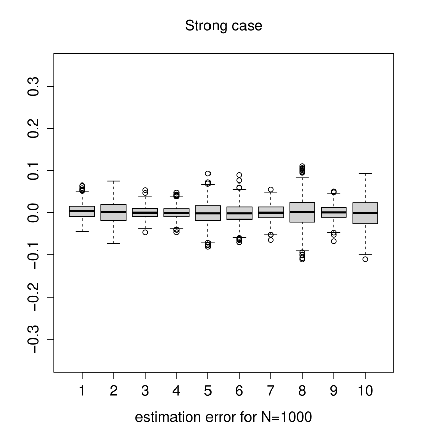
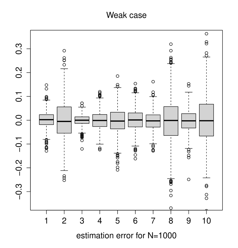
Figure 1: The least squares estimator of $1000$ independent simulations of model (43) with unknown parameter given in Table 1, when the noise is strong (left panels) and when the noise is weak (right panels). The panels display the distribution of the estimation errors $\hat{\mathbf{\Phi}}_{ii}(\nu)-\mathbf{\Phi}_{ii}(\nu)$, for $i=1,2$ and $\nu=1,\dots,5$.

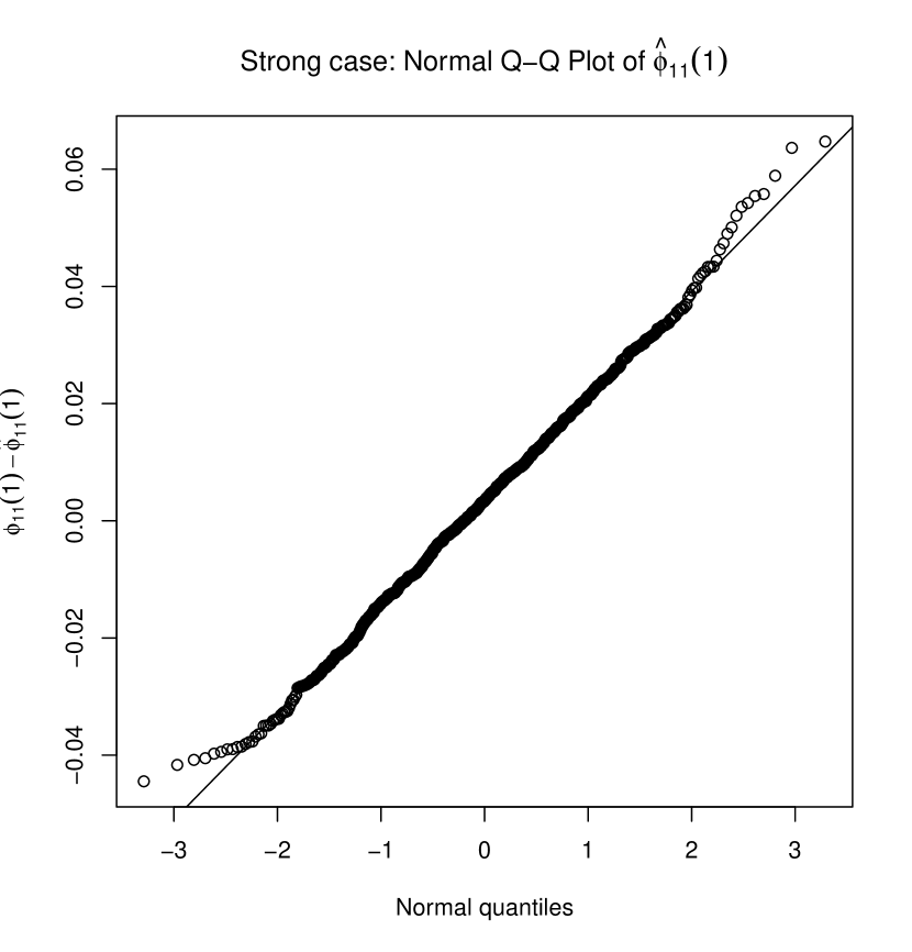
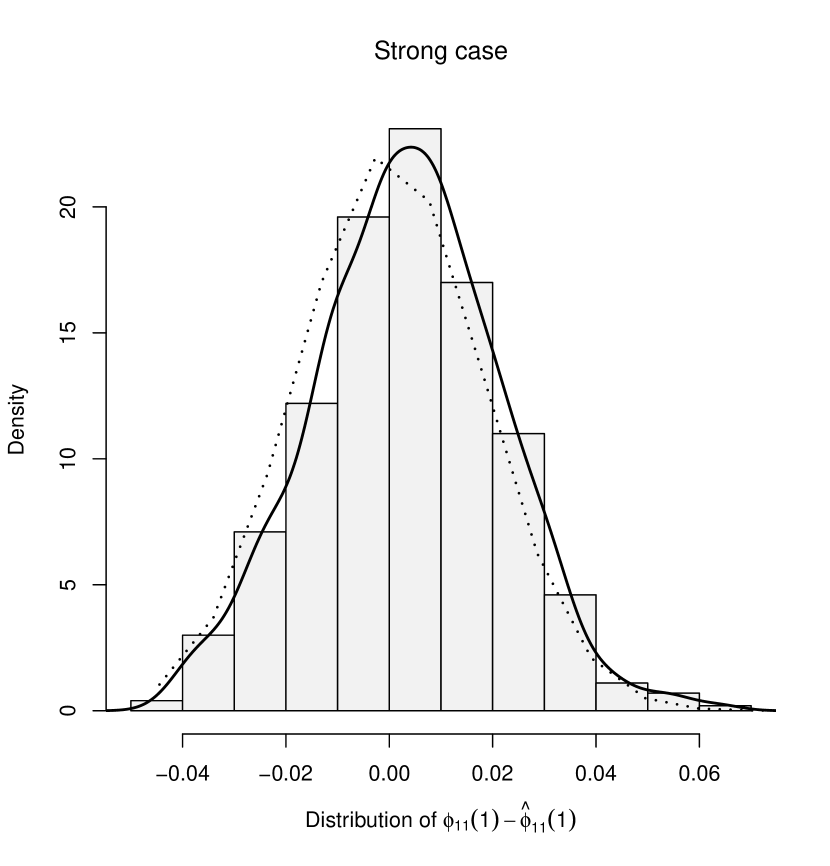
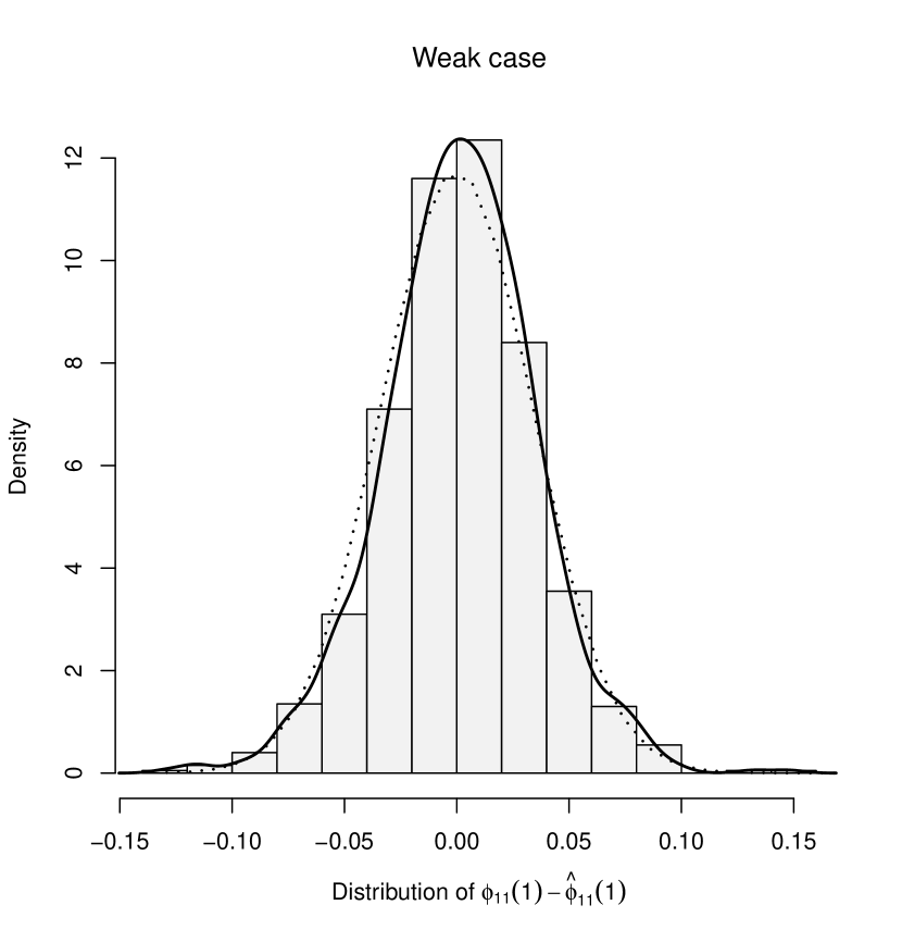
Figure 2: The least squares estimator of $1000$ independent simulations of the model (43) with size $N=1000$ and unknown parameter given in Table 1, when the noise is strong (left panels) and when the noise is weak (right panels). The panels of the top present the Q–Q plot of the estimates $\mathbf{\Phi}_{11}(1)$. The bottom panels display the distribution of the same estimates. The kernel density estimate is displayed in full line, and the centered Gaussian density with the same variance is plotted in dotted line.

Figures 1 and 2 compare the distribution of the least squares estimator in the strong and weak noise cases. The distributions of $\hat{\mathbf{\Phi}}_{ii}(\nu)$, for $i=1,2$ and $\nu=1,\dots,5$ are more accurate in the strong case than in the weak one. Similar simulation experiments, not reported here, reveal that the situation is opposite, that is the least squares estimators of $\hat{\Phi}_{ii}(\nu)$ are more accurate in the weak case than in the strong case, when the weak noise is defined by $\epsilon_{i,ns+\nu}=\eta_{i,ns+\nu}(|\eta_{i,ns+\nu-1}|+1)^{-1}$ for $i=1,2$. This is in accordance with the univariate results of Romano and Thombs (1996) who showed that, with similar noises, the asymptotic variance of the sample autocorrelations can be greater or less than 1 as well (1 is the asymptotic variance for strong white noises). Figure 2 compares the distribution of $\mathbf{\Phi}_{11}(1)$ in the strong and weak noise cases. We consider here (one of) the parameter which variance’s seems to have problems in the weak case, when we use the standard estimator $\hat{\mathbf{\Theta}}_{S}(\nu)$.

Figure 3 compares the standard estimator $\hat{\bf\Theta}_{S}(\nu)$ with the proposed sandwich estimators based on spectral density estimation $\hat{\bf\Theta}^{\mathrm{{SP}}}(\nu)$ or on kernel methods $\hat{\bf\Theta}^{\mathrm{{HAC}}}(\nu)$ of the asymptotic variance $\bf\Theta(\nu)$. We used the spectral estimator $\hat{\mathbf{\Psi}}=\hat{\mathbf{\Psi}}^{\mathrm{{SP}}}$ defined in Theorem 4.1 where the AR order $r$ is automatically selected by AIC, using the function VARselect() of the vars R package. Note that similar simulation experiments, not reported here, reveal that the performance of the proposed estimator is least sensitive to the choice of others criteria such that: BIC, HQ and FPE. The HAC estimator based on kernel methods $\hat{\mathbf{\Psi}}=\hat{\mathbf{\Psi}}^{\mathrm{{HAC}}}$ defined in Theorem 4.2 is also used. HAC estimators have been the focus of extensive research in the time series literature. Contributions to this research in the econometrics literature include, among others, Newey and West (1987), Andrews (1991), Müller (2014) and Lazarus et al. (2018).The bandwidth selection for the HAC estimation is an important practical issue. For kernel densities with unit-interval support, the bandwidth parameter, is often called the lag-truncation parameter. Based on theoretical results in Andrews (1991), the practice is to choose a small value for the lag-truncation parameter. More recently, it has been shown that this standard approach can often lead to tests which incorrectly reject the null hypothesis (Müller, 2014). Much of the literature remains in the Newey-West framework but uses very long lag-truncation parameter (Kiefer and Vogesland, 2002). As indicated by Francq and Zakoïan (2007), ”it is well known that choice of bandwidth equal to the sample size (i.e. $b_{N}=1/N$ in our case) results in inconsistent LRV estimators”. In our case it is crucial to have a consistent estimator of the matrix $\mathbf{\Psi}(\nu)$.

Several leading lag-truncation choices based on traditional Newey-West HAC estimators are:

• $b_{N}=1/\ln{(N)}$, as proposed by Francq and Zakoïan (2000).

• $b_{N}=1/\left(\lfloor 4(N/100)^{2/9}\rfloor+1\right)$ or $b_{N}=1/\left(\lfloor N^{1/4}\rfloor+1\right)$.

  This choice is a standard textbook recommendation (Wooldridge, 2015).

• $b_{N}=1/\left(\lfloor 0.75N^{1/3}\rfloor+1\right)$. This rule derives from a formula of Andrews (1991), in the case of a first order autoregressive model.

• $b_{N}=1/\left(\lfloor 1.3N^{1/2}\rfloor+1\right)$, as proposed by Lazarus et al. (2018). Its use of $N^{1/2}$ produces higher truncation lags. For example, if $N=1000$, then $b_{N}=1/43$.

• $b_{N}=1/N$, as proposed by Kiefer and Vogesland (2002).

The performance of Newey-West estimators depends on the choice of the kernel function and lag-truncation. We focused our investigation to weight function $f:\mathbb{R}\to\mathbb{R}$ which is bounded, with compact support $[-a,a]$ and continuous at the origin with $f(0)=1$. Such weight functions are for instance: Bartlett, Truncated, Parzen and Quadratic Spectral kernels. To determine the optimal lag-truncation parameter and the kernel, a $10$-fold cross-validation is used. In the density estimation literature, the cross-validation method has been suggested by Beltrão and Bloomfield (1987) or by Whaba and Wold (1975). For the bandwidth, we chose $30$ values between $1/50$ and $1/6$ and four kernels were investigated: Bartlett, Truncated, Parzen and Quadratic Spectral. The best results, for our simulated data, was obtained using the Bartlett kernel with a bandwidth equal to $1/21$.

In the strong PVAR case we know that the three estimators are consistent. In view of the three top panels of Figure 3, it seems that the standard estimator is most accurate than the proposed sandwich estimators in the strong case. This is not surprising because the spectral estimator or the HAC estimator are more robust, in the sense that these estimators continue to be consistent in the weak PVAR case, contrary to the standard estimator. It is clear that in the weak case $NVar(\hat{\mathbf{\Phi}}_{ii}(\nu)-\mathbf{\Phi}_{ii}(\nu))^{2}$ is better estimated by $\hat{\mathbf{\Theta}}_{ii}^{\mathrm{{SP}}}(\nu)$ or by $\hat{\bf\Theta}_{ii}^{\mathrm{{HAC}}}(\nu)$ (see the box-plots $1,2,\dots,10$ of the center-bottom and the right-bottom panel of Figure 3) than by $\hat{\mathbf{\Theta}}_{S}(\nu)$ (see the box-plots $1,2,\dots,10$ of the left-bottom panel), for $i=1,2$ and $\nu=1,\dots,5$. The failure of the standard estimator of $\mathbf{\Theta}$ in the weak PVAR setting may have important consequences in terms of hypothesis testing for instance.

Table 3 displays the empirical sizes of the standard Wald test and that of the modified versions proposed in Section 5. We use $3$ nominal levels $\alpha=1\%$, 5% and 10%. For these nominal levels, the empirical relative frequency of rejection size over the $1000$ independent replications should vary respectively within the confidence intervals $[0.3\%,1.7\%]$, $[3.6\%,6.4\%]$ and $[8.1\%,11.9\%]$ with probability 95% and $[0.3\%,1.9\%]$, $[3.3\%,6.9\%]$ and $[7.6\%,12.5\%]$ with probability 99% under the assumption that the true probabilities of rejection are respectively $\alpha=1\%$, $\alpha=5\%$ and $\alpha=10\%$. When the relative rejection frequencies are outside the significant limits with probability 95%, they are displayed in bold type in Table 3. For the strong PVAR model I, the relative rejection frequencies are inside the significant limits. For the weak PVAR model II, the relative rejection frequencies of the standard Wald test are definitely outside the significant limits. It may lead the statistician to wrongly reject the hypothesis that $H_{0}:\mathbf{\Phi}_{22}(\nu)=0$ for $\nu=1,\dots,5$ if he does not take into account the dependence of the errors $\epsilon$. Thus the error of first kind is well controlled by all the tests in the strong case, but only by the modified versions of the Wald tests in the weak case when $N$ increases. We draw the conclusion that the modified versions are preferable to the standard ones. Table 5 shows that the powers of all the tests are very similar in the strong PVAR model III. The same is also true for the two modified Wald tests in the weak PVAR model IV. The empirical powers of the standard Wald tests are hardly interpretable for Model IV, because we have already seen in Table 3 that the standard Wald test does not well controls the error of first kind in the weak PVAR framework.

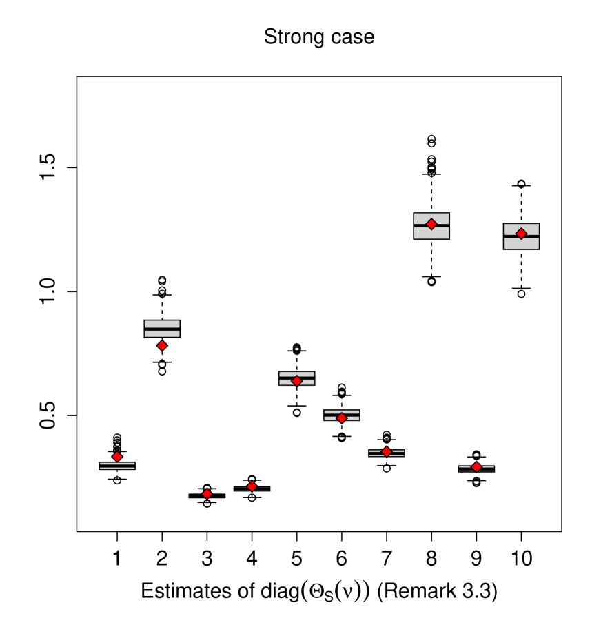
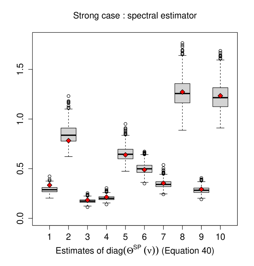
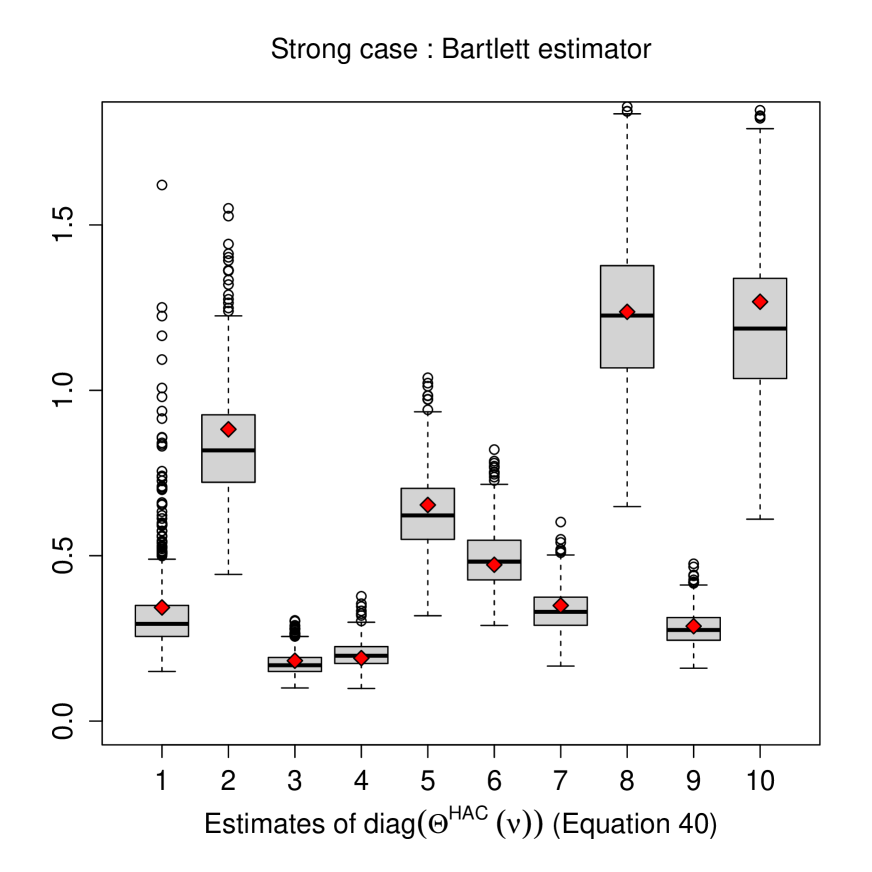
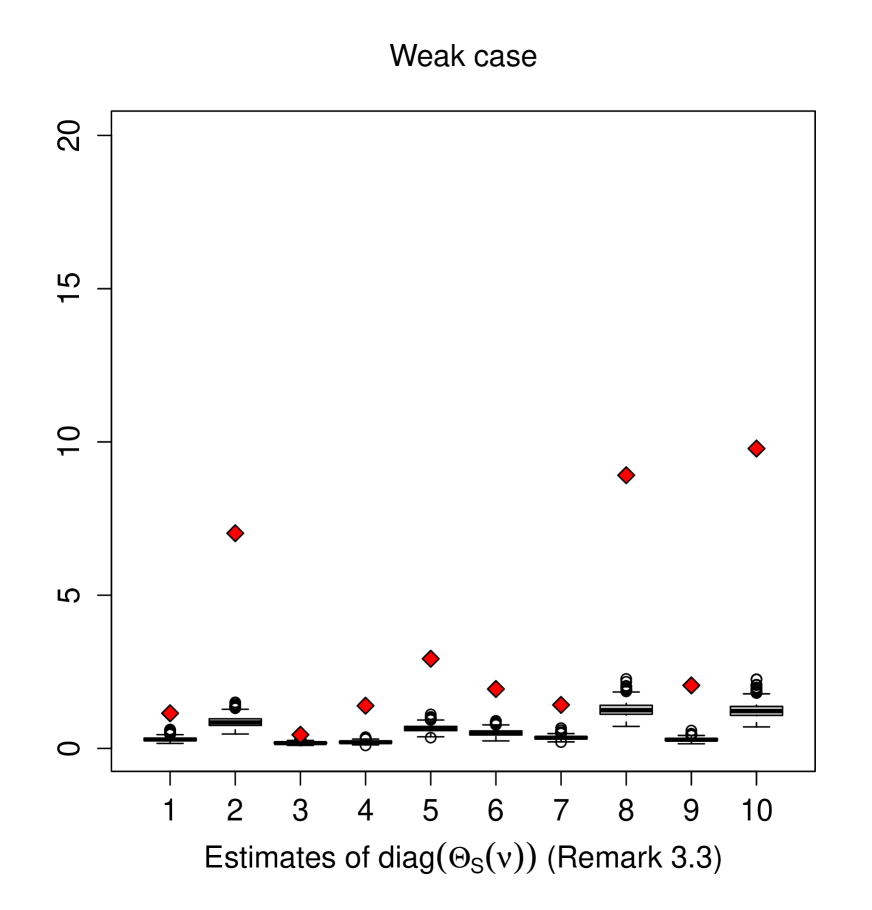
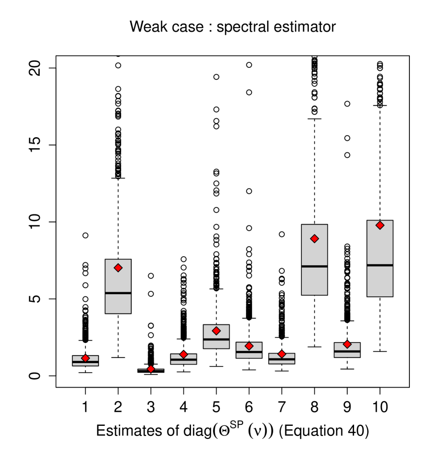
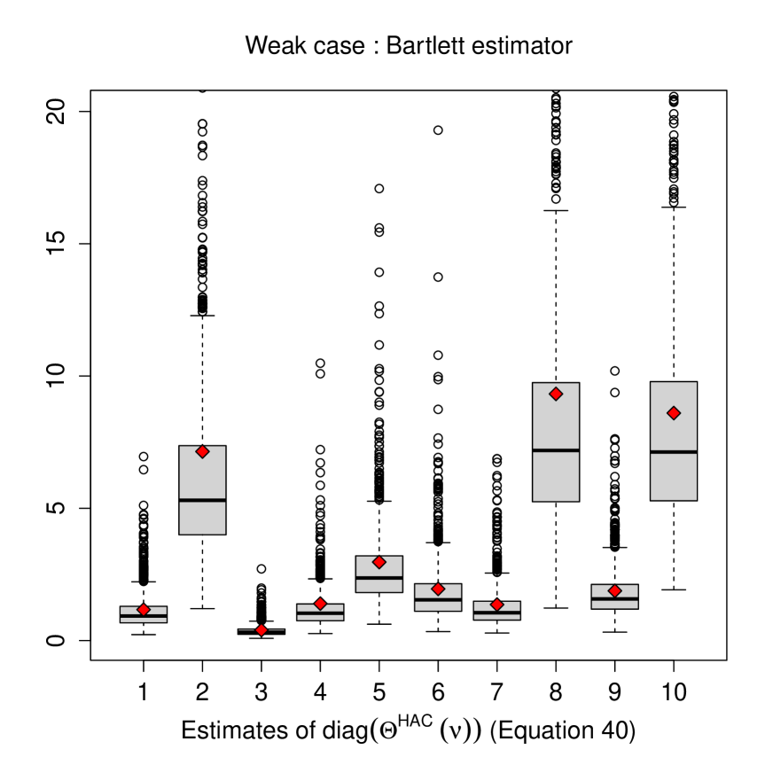
Figure 3: Comparison of standard and modified estimates of the asymptotic variance of the least squares estimator of the model parameters, on the simulated models presented in Figure 1. The diamond symbols represent the mean, over $1000$ replications, of the standardized squared errors $N\left(\hat{\mathbf{\Phi}}_{11}(1)-\mathbf{\Phi}_{11}(1)\right)^{2}$ for 1 (0.33 in the strong case and 1.15 in the weak case), $N\left(\hat{\mathbf{\Phi}}_{22}(1)-\mathbf{\Phi}_{22}(1)\right)^{2}$ for 2 (0.78 in the strong case and 7.02 in the weak case), $N\left(\hat{\mathbf{\Phi}}_{11}(2)-\mathbf{\Phi}_{11}(2)\right)^{2}$ for 3 (0.18 in the strong case and 0.45 in the weak case), $N\left(\hat{\mathbf{\Phi}}_{22}(2)-\mathbf{\Phi}_{22}(2)\right)^{2}$ for 4 (0.21 in the strong case and 1.39 in the weak case), $N\left(\hat{\mathbf{\Phi}}_{11}(3)-\mathbf{\Phi}_{11}(3)\right)^{2}$ for 5 (0.64 in the strong case and 2.93 in the weak case), $N\left(\hat{\mathbf{\Phi}}_{22}(3)-\mathbf{\Phi}_{22}(3)\right)^{2}$ for 6 (0.49 in the strong case and 1.94 in the weak case), $N\left(\hat{\mathbf{\Phi}}_{11}(4)-\mathbf{\Phi}_{11}(4)\right)^{2}$ for 7 (0.35 in the strong case and 1.42 in the weak case), $N\left(\hat{\mathbf{\Phi}}_{22}(4)-\mathbf{\Phi}_{22}(4)\right)^{2}$ for 8 (1.27 in the strong case and 8.91 in the weak case), $N\left(\hat{\mathbf{\Phi}}_{11}(5)-\mathbf{\Phi}_{11}(5)\right)^{2}$ for 9 (0.29 in the strong case and 2.06 in the weak case) and $N\left(\hat{\mathbf{\Phi}}_{22}(5)-\mathbf{\Phi}_{22}(5)\right)^{2}$ for 10 (1.23 in the strong case and 9.79 in the weak case) .

Table 3: Empirical size of standard and modified tests: relative frequencies (in %) of rejection of $H_{0}:\mathbf{\Phi}_{22}(\nu)=0$ for $\nu=1,\dots,5$. Modified Wald Test (41), which use the spectral estimator or the HAC estimator denoted: $\mathrm{{W}}_{N}^{\mathrm{SP}}(\nu)$ or $\mathrm{{W}}_{N}^{\mathrm{HAC}}(\nu)$. The number of replications is $1000$.

Model	Length $N$	Level	$\mathrm{{W}}_{N}^{\ast}(\nu)$					$\mathrm{{W}}_{N}^{\mathrm{SP}}(\nu)$					$\mathrm{{W}}_{N}^{\mathrm{HAC}}(\nu)$
			$\nu$					$\nu$					$\nu$
			$1$	$2$	$3$	$4$	$5$	$1$	$2$	$3$	$4$	$5$	$1$	$2$	$3$	$4$	$5$
		$\alpha=1\%$	0.8	0.1	0.9	0.8	1.3	0.8	0.7	0.9	1.2	1.0	0.8	0.7	1.0	1.2	1.1
I	$N=1,000$	$\alpha=5\%$	4.5	3.4	4.2	4.7	6.2	5.2	5.1	5.3	6.0	6.5	5.0	5.3	5.4	6.1	6.4
		$\alpha=10\%$	9.6	8.3	10.2	11.5	10.1	10.1	11.1	12.2	12.1	10.3	9.8	11.0	11.9	11.8	10.5
		$\alpha=1\%$	0.8	0.4	1.0	1.1	0.7	0.9	1.1	1.3	1.0	0.9	1.0	1.2	1.3	1.0	0.8
I	$N=4,000$	$\alpha=5\%$	4.8	4.8	4.0	5.6	4.6	4.8	5.6	5.7	6.0	4.6	5.0	5.8	5.7	6.1	4.5
		$\alpha=10\%$	9.6	9.2	9.8	10.5	9.8	9.8	11.2	11.6	11.1	9.7	10.0	11.7	11.4	11.0	10.1
		$\alpha=1\%$	35.2	31.9	33.0	36.4	34.3	2.1	1.4	2.0	2.0	1.2	2.1	1.3	1.4	1.5	1.1
II	$N=1,000$	$\alpha=5\%$	46.6	44.5	45.5	51.3	45.6	6.3	6.2	7.9	6.5	6.9	6.6	6.1	6.6	6.1	6.5
		$\alpha=10\%$	54.6	51.9	52.9	57.9	53.2	12.5	11.2	13.2	12.7	12.2	11.5	10.8	13.0	12.2	11.4
		$\alpha=1\%$	38.6	32.2	33.3	39.7	36.8	1.1	1.4	1.4	1.4	0.5	1.0	1.3	1.4	1.2	0.5
II	$N=4,000$	$\alpha=5\%$	51.9	46.7	46.3	52.0	48.6	5.9	5.6	5.2	5.8	4.4	6.0	5.5	4.8	6.0	4.2
		$\alpha=10\%$	57.5	54.1	53.1	57.5	55.1	11.1	11.1	10.5	11.9	9.6	10.4	10.4	10.8	11.8	9.0
I: Strong PVAR$(1)$ model (43)-(44) with unknown parameter given in Table 4.
II: Weak PVAR$(1)$ model (43)-(45) with unknown parameter given in Table 4.

Table 4: Parameters of DGP models used in the simulation to test $H_{0}:\mathbf{\Phi}_{22}(\nu)=0$ for $\nu=1,\dots,5$.

MODEL		$\mathbf{\Phi}(1)$			$\mathbf{\Phi}(2)$			$\mathbf{\Phi}(3)$			$\mathbf{\Phi}(4)$			$\mathbf{\Phi}(5)$
DGP		-1.43	0.00		0.46	0.00		1.23	0.00		0.30	0.00		0.90	0.00
		0.00	0.00		0.00	0.00		0.00	0.00		0.00	0.00		0.00	0.00

Table 5: Empirical power of standard and modified tests: relative frequencies (in %) of rejection of $H_{0}:\mathbf{\Phi}_{22}(\nu)=0$ for $\nu=1,\dots,5$. Modified Wald Test (41), which use the spectral estimator or the HAC estimator denoted: $\mathrm{{W}}_{N}^{\mathrm{SP}}(\nu)$ or $\mathrm{{W}}_{N}^{\mathrm{HAC}}(\nu)$. The number of replications is $1000$.

Model	Length $N$	Level	$\mathrm{{W}}_{N}^{\ast}(\nu)$					$\mathrm{{W}}_{N}^{\mathrm{SP}}(\nu)$					$\mathrm{{W}}_{N}^{\mathrm{HAC}}(\nu)$
			$\nu$					$\nu$					$\nu$
			$1$	$2$	$3$	$4$	$5$	$1$	$2$	$3$	$4$	$5$	$1$	$2$	$3$	$4$	$5$
		$\alpha=1\%$	79.0	100.0	44.8	51.4	54.7	78.8	100.0	49.2	52.0	55.2	78.8	100.0	48.7	52.1	54.7
III	$N=4,000$	$\alpha=5\%$	93.3	100.0	67.9	75.1	76.4	93.1	100.0	70.1	75.1	76.9	93.0	100.0	70.3	75.2	76.6
		$\alpha=10\%$	97.1	100.0	77.2	82.7	84.8	97.4	100.0	78.7	83.0	85.0	97.3	100.0	78.5	83.2	84.9
		$\alpha=1\%$	59.3	85.4	52.3	54.5	54.0	7.8	30.7	6.5	5.2	5.2	7.4	30.3	5.8	5.4	5.1
IV	$N=4,000$	$\alpha=5\%$	68.4	90.8	63.6	66.3	64.1	23.4	53.4	17.7	16.9	15.4	22.4	53.1	17.7	16.2	15.0
		$\alpha=10\%$	74.4	92.9	69.3	71.7	71.7	32.8	65.6	27.1	25.7	24.3	32.0	66.0	27.4	25.2	24.2
III: Strong PVAR$(1)$ model (43)-(44) with unknown parameter given in Table 6.
IV: Weak PVAR$(1)$ model (43)-(45) with unknown parameter given in Table 6.

Table 6: Parameters of DGP models used in the simulation of empirical power to test $H_{0}:\mathbf{\Phi}_{22}(\nu)=0$ for $\nu=1,\dots,5$.

MODEL		$\mathbf{\Phi}(1)$			$\mathbf{\Phi}(2)$			$\mathbf{\Phi}(3)$			$\mathbf{\Phi}(4)$			$\mathbf{\Phi}(5)$
DGP		-1.43	0.00		0.46	0.00		1.23	0.00		0.30	0.00		0.90	0.00
		0.00	0.05		0.00	0.05		0.00	0.05		0.00	0.05		0.00	0.05

7 Application to real data

In this section, we consider the daily returns of two European stock market indices: CAC 40 (Paris) and DAX (Frankfurt), from March $3$, $1990$ to March $10$, $2022$. The data were obtained from Yahoo Finance. Because of the legal holidays, many weeks comprise less than five observations. We preferred removing the entire weeks when there was less than five data available, giving a bivariate time series of sample size equal to $7060$. The period $\nu=5$ is naturally selected.

In order to analyse these two European indices, we fitted a PVAR model of order $1$ to the bivariate series of observations:

$$\mathbf{Y}_{ns+\nu}=\mathbf{\Phi}(\nu)\mathbf{Y}_{ns+\nu-1}+\mbox{\boldmath$\epsilon$}_{ns+\nu}\quad\nu=1,\ldots,5,$$

where $\mathbf{Y}_{t}=\left(r_{t}^{1},r_{t}^{2}\right)^{\top}$ and $r_{t}^{1}$, $r_{t}^{2}$ represents the log-return of CAC 40 and DAX respectively. The log-return is defined as $r_{t}=100\times\ln{(I_{t}/I_{t-1})}$ where $I_{t}$ represents the value of the index at time $t$. Seasonal means are first removed from the series, meaning that a model is formulated by examining $\mathbf{Y}_{ns+\nu}-\mbox{\boldmath$\mu$}(\nu)$. The two time series of log-returns are displayed in Figure 4.

We present in Table 7 the estimated parameters $\hat{\mbox{\boldmath$\beta$}}=(\hat{\mbox{\boldmath$\beta$}}(1),\dots,\hat{\mbox{\boldmath$\beta$}}(5))^{\top}$ and their estimated standard error proposed in the strong case (see Remark 3.3) denoted $\hat{\sigma}_{\mathrm{S}}$ and the weakly consistent estimators proposed (37) and (38), denoted respectively by $\hat{\sigma}_{\mathrm{{SP}}}$ and $\hat{\sigma}_{\mathrm{{HAC}}}$; $\hat{\mbox{\boldmath$\Sigma$}}(\nu)$ represents the estimated variance of residuals $\hat{\mbox{\boldmath$\epsilon$}}(\nu)$. The $p$-values of the $t$-statistic of $\hat{\mbox{\boldmath$\beta$}}$ and those of the standard and modified versions of the Wald tests are denoted: pval_S, pval_SP, pval_HAC, pval${}^{\mathrm{{W}}}_{S}$, pval${}^{\mathrm{{W}}}_{\mathrm{{SP}}}$ and pval${}^{\mathrm{{W}}}_{\mathrm{{HAC}}}$, where the exponent W stands for Wald. The $p$-values less than 5% are in bold, those less than 1% are underlined. The autoregressive coefficients $\hat{\mathbf{\Phi}}_{ij}(\nu)$ for $i,j=1,2$ are rather small on Monday, Tuesday and Friday. Four of them are significant at the 1% level in the strong case on Wednesday and Thursday. In the weak case, none of them are significant at the 1% level. This is in accordance with the results of Francq et al. (2011) who showed that the log-returns of these two European stock market indices constitute the weak periodic white noises. As in Francq et al. (2011), the estimated variance of residuals shows that, the volatility is considerably greater on Monday and smaller for the other days.

Figure 4: Log-returns of CAC 40 (Paris) and DAX (Frankfurt)

Table 7: Least squares estimators used to fit the log-returns of CAC 40 and DAX data to a bivariate PVAR model with $\nu=5$; the $\hat{\sigma}_{\mathrm{S}}$, $\hat{\sigma}_{\mathrm{{SP}}}$ and $\hat{\sigma}_{\mathrm{{HAC}}}$ represent the standard errors in the strong case and for our proposed estimators in the weak case; pval_S, pval_SP, pval_HAC, pval${}^{\mathrm{{W}}}_{S}$, pval${}^{\mathrm{{W}}}_{\mathrm{{SP}}}$ and pval${}^{\mathrm{{W}}}_{\mathrm{{HAC}}}$ correspond to the $p$-values of the $t$-statistic of $\hat{\mbox{\boldmath$\beta$}}$ and those of the standard and modified versions of the Wald tests are also presented; $\hat{\mbox{\boldmath$\Sigma$}}_{\mbox{\boldmath$\epsilon$}}(\nu)$ represents the estimated variance of residuals $\hat{\mbox{\boldmath$\epsilon$}}(\nu)$. The $p$-values less than 5% are in bold, those less than 1% are underlined.

	$\hat{\mbox{\boldmath$\beta$}}$	$\hat{\sigma}_{\mathrm{S}}$	$\hat{\sigma}_{\mathrm{{SP}}}$	$\hat{\sigma}_{\mathrm{{HAC}}}$	pvalS	pvalSP	pvalHAC	pval${}^{\mathrm{{W}}}_{S}$	pval${}^{\mathrm{{W}}}_{\mathrm{{SP}}}$	pval${}^{\mathrm{{W}}}_{\mathrm{{HAC}}}$	$\mbox{{vec}}{\left(\hat{\mbox{\boldmath$\Sigma$}}_{\mbox{\boldmath$\epsilon$}}(\nu)\right)}$
1	-0.0349	0.0707	0.1456	0.1078	0.6220	0.8107	0.7464	0.6219	0.8107	0.7464	3.5457
2	0.0153	0.0731	0.1480	0.1152	0.8346	0.9180	0.8947	0.8346	0.9179	0.8947	3.2404
3	-0.0070	0.0706	0.0992	0.0862	0.9215	0.9441	0.9357	0.9215	0.9441	0.9357	3.2404
4	-0.0378	0.0729	0.1019	0.1004	0.6044	0.7106	0.7066	0.6043	0.7106	0.7065	3.7859
5	-0.0506	0.0399	0.0524	0.0486	0.2045	0.3339	0.2975	0.2043	0.3337	0.2973	1.7366
6	-0.0270	0.0420	0.0663	0.0622	0.5214	0.6843	0.6651	0.5213	0.6842	0.6650	1.5938
7	-0.0020	0.0386	0.0551	0.0474	0.9591	0.9713	0.9667	0.9591	0.9713	0.9667	1.5938
8	-0.0246	0.0407	0.0742	0.0624	0.5450	0.7399	0.6932	0.5449	0.7398	0.6931	1.9297
9	-0.3001	0.0532	0.1296	0.1200	0.0000	0.0207	0.0125	0.0000	0.0206	0.0124	1.6817
10	-0.1256	0.0545	0.0781	0.0693	0.0214	0.1078	0.0704	0.0213	0.1076	0.0702	1.4736
11	0.2605	0.0505	0.1381	0.1265	0.0000	0.0595	0.0396	0.0000	0.0592	0.0394	1.4736
12	0.0360	0.0517	0.0607	0.0642	0.4869	0.5535	0.5752	0.4868	0.5534	0.5751	1.7671
13	-0.1498	0.0548	0.1020	0.0844	0.0063	0.1422	0.0761	0.0062	0.1420	0.0758	2.0261
14	-0.0744	0.0551	0.0639	0.0715	0.1767	0.2445	0.2979	0.1765	0.2443	0.2977	1.7907
15	0.1862	0.0538	0.1021	0.0855	0.0006	0.0683	0.0295	0.0005	0.0681	0.0294	1.7907
16	0.0955	0.0541	0.0620	0.0715	0.0778	0.1240	0.1824	0.0776	0.1237	0.1822	2.0471
17	-0.0227	0.0521	0.0681	0.0647	0.6627	0.7385	0.7252	0.6626	0.7384	0.7251	1.7824
18	-0.0055	0.0522	0.0670	0.0654	0.9156	0.9343	0.9326	0.9156	0.9343	0.9326	1.5118
19	0.0694	0.0520	0.0739	0.0699	0.1823	0.3480	0.3209	0.1821	0.3479	0.3207	1.5118
20	0.0420	0.0521	0.0734	0.0705	0.4202	0.5677	0.5517	0.4201	0.5676	0.5516	1.7861

8 Conclusions

In this work, we have established under mild assumptions, the asymptotic distribution of the least squares estimator of the model parameters in PVAR time series models with dependent but uncorrelated errors. Our results extend Theorem 1 of Ursu and Duchesne (2009) for PVAR models with independent errors. Note that if $s=1$, we retrieve the result on weak VAR obtained by Francq and Raïssi (2007). The asymptotic covariance matrix of the least squares estimators obtained under independent errors is generally not consistent in the weak PVAR case. For statistical inference problem, including in particular, the significance tests on the parameters, the assumption of independent errors can be quite misleading when analysing data from PVAR models with dependent errors.

We proposed two estimators of the asymptotic variance matrix: the spectral density estimator and the heteroskedasticity and autocorrelation consistent estimator based on kernel methods. The empirical results of Sections 6 and 7 illustrate the applicability of our theoretical results using a consistent estimator of the asymptotic variance matrix of the least square estimators of weak PVAR parameters. In future works, we intend to study how the existing identification and diagnostic checking (see e.g. Ursu and Duchesne (2009)) procedures should be adapted in the weak PVAR framework considered in the present paper. The asymptotic covariance matrix of the least squares estimators of a weak PVAR model is no longer block diagonal with respect to seasons and depends on the fourth-order moments of the innovation process (through the matrix $\mathbf{\Psi}(\nu)$).

Appendix A Appendix : Proofs of the main results

The proof of Theorem 3.1 is quite technical. This is adaptation of the arguments used in Francq et al. (2011).

A.1 Proof of Theorem 3.1

The proof is quite long so we divide it in several steps.

$\diamond$ Step 1: preliminaries

In view of (3), it is easy to see that $\mathbf{X}_{n}^{\top}(\nu)$ is a measurable function of the random vectors $\{\mbox{\boldmath$\epsilon$}_{ns+\nu-k},k\geq 1\}$. Thus the assumption (A2) of the error term $(\mbox{\boldmath$\epsilon$}_{n}^{\ast})_{n\in\mathbb{Z}}$ allows us to show that $(\mbox{{vec}}\{\mbox{\boldmath$\epsilon$}_{ns+\nu}\mathbf{X}_{n}^{\top}(\nu)\})_{n\in\mathbb{Z}}$ is a stationary and ergodic sequence. Applying the ergodic theorem, we obtain that

$$N^{-1}\sum_{n=0}^{N-1}\mbox{{vec}}\{\mbox{\boldmath$\epsilon$}_{ns+\nu}\mathbf{X}_{n}^{\top}(\nu)\}\stackrel{{\scriptstyle a.s.}}{{\to}}\mathbb{E}\left[\mbox{{vec}}\{\mbox{\boldmath$\epsilon$}_{ns+\nu}\mathbf{X}_{n}^{\top}(\nu)\}\right]=\mathbf{0},$$ (46)

by using the non-correlation between $\mbox{\boldmath$\epsilon$}_{ns+\nu}$’s (see (A0)) and where $\mathbf{0}$ is the $\{d^{2}p(\nu)\}\times 1$ null vector.

$\diamond$ Step 2: convergence in distribution of $N^{-1/2}\sum_{n=0}^{N-1}\mbox{{vec}}\{\mbox{\boldmath$\epsilon$}_{ns+\nu}\mathbf{X}_{n}^{\top}(\nu)\}$

Using the stationarity of $(\mbox{{vec}}\{\mbox{\boldmath$\epsilon$}_{ns+\nu}\mathbf{X}_{n}^{\top}(\nu)\})_{n\in\mathbb{Z}}$, we have

var $$\left\{\frac{1}{\sqrt{N}}\sum_{n=0}^{N-1}\mbox{{vec}}\{\mbox{\boldmath$\epsilon$}_{ns+\nu}\mathbf{X}_{n}^{\top}(\nu)\}\right\}$$

$$=\frac{1}{N}\sum_{n=0}^{N-1}\sum_{n^{\prime}=0}^{N-1}\mbox{cov}\left\{\mbox{{vec}}\{\mbox{\boldmath$\epsilon$}_{ns+\nu}\mathbf{X}_{n}^{\top}(\nu)\},\mbox{{vec}}\{\mbox{\boldmath$\epsilon$}_{n^{\prime}s+\nu}\mathbf{X}_{n^{\prime}}^{\top}(\nu)\}\right\}$$

$$=\frac{1}{N}\sum_{h=-N+1}^{N-1}\left(N-|h|\right)c(\nu,h),$$

where

$$c(\nu,h)=\mbox{cov}\left(\mbox{{vec}}\{\mbox{\boldmath$\epsilon$}_{ns+\nu}\mathbf{X}_{n}^{\top}(\nu)\},\mbox{{vec}}\{\mbox{\boldmath$\epsilon$}_{(n-h)s+\nu}\mathbf{X}_{n-h}^{\top}(\nu)\}\right).$$

By the dominated convergence theorem, it follows that

$$\mathbf{\Psi}(\nu)=\sum_{h=-\infty}^{\infty}\mbox{cov}\left(\mbox{{vec}}\{\mbox{\boldmath$\epsilon$}_{ns+\nu}\mathbf{X}_{n}^{\top}(\nu)\},\mbox{{vec}}\{\mbox{\boldmath$\epsilon$}_{(n-h)s+\nu}\mathbf{X}_{n-h}^{\top}(\nu)\}\right).$$

The existence of the last sum is a consequence of (A3) and the Davydov (1968) inequality. Using (46) and the elementary relations $\mbox{{vec}}(ab^{\top})=b\otimes a$ for any vectors $a$ and $b$, and $(A\otimes B)(C\otimes D)=(AC)\otimes(BD)$ for matrices of appropriate sizes (see Lütkepohl (2005)), it follows that

$$\mathbf{\Psi}(\nu)=\sum_{h=-\infty}^{\infty}\mathbb{E}\left(\mathbf{X}_{n}(\nu)\mathbf{X}_{n-h}^{\top}(\nu)\otimes\mbox{\boldmath$\epsilon$}_{ns+\nu}\mbox{\boldmath$\epsilon$}_{(n-h)s+\nu}^{\top}\right).$$

Let $\mbox{\boldmath$\epsilon$}_{n}(\nu)=(\mbox{\boldmath$\epsilon$}_{ns+\nu-1}^{\top},\ldots,\mbox{\boldmath$\epsilon$}_{ns+\nu-p(\nu)}^{\top})^{\top}$, $n=0,1,\ldots,N-1$, be a $\{dp(\nu)\}\times 1$ random vectors. In the sequel, we need the elementary identity $\mbox{{vec}}(ABC)=(I\otimes AB)\mbox{{vec}}(C)$ (see Lütkepohl (2005)). In view of (3), we have for all $r\geq 0$

$$\mbox{{vec}}\{\mbox{\boldmath$\epsilon$}_{ns+\nu}\mathbf{X}_{n}^{\top}(\nu)\} =\sum_{i=0}^{\infty}\left(\mathbf{I}_{dp(\nu)}\otimes\mbox{\boldmath$\epsilon$}_{ns+\nu}\mbox{\boldmath$\epsilon$}_{n-i}^{\top}(\nu)\right)\mbox{{vec}}\left(\mathbf{I}_{p(\nu)}\otimes\mathbf{C}_{i}^{\top}(\nu)\right)$$

$$=\mathbf{W}_{n,r}(\nu)+\mathbf{U}_{n,r}(\nu),$$ (47)

where

$$\mathbf{W}_{n,r}(\nu) =\sum_{i=0}^{r}\left(\mathbf{I}_{dp(\nu)}\otimes\mbox{\boldmath$\epsilon$}_{ns+\nu}\mbox{\boldmath$\epsilon$}_{n-i}^{\top}(\nu)\right)\mbox{{vec}}\left(\mathbf{I}_{p(\nu)}\otimes\mathbf{C}_{i}^{\top}(\nu)\right)$$

$$\mathbf{U}_{n,r}(\nu) =\sum_{i=r+1}^{\infty}\left(\mathbf{I}_{dp(\nu)}\otimes\mbox{\boldmath$\epsilon$}_{ns+\nu}\mbox{\boldmath$\epsilon$}_{n-i}^{\top}(\nu)\right)\mbox{{vec}}\left(\mathbf{I}_{p(\nu)}\otimes\mathbf{C}_{i}^{\top}(\nu)\right).$$

The processes $(\mathbf{W}_{n,r}(\nu))_{n\in\mathbb{Z}}$ and $(\mathbf{U}_{n,r}(\nu))_{n\in\mathbb{Z}}$ are stationary and centered. Moreover, under Assumption (A3) and $r$ fixed, the process $(\mathbf{W}_{n,r}(\nu))_{n\in\mathbb{Z}}$ is strongly mixing (see Theorem 14.1 in Davidson (1994)), with mixing coefficients $\alpha_{\mathbf{W}_{r}}(h)\leq\alpha_{\mbox{\boldmath$\epsilon$}}\left(\max\{0,h-1\}\right)$. Thus (A3) implies $\sum_{h=0}^{\infty}\{\alpha_{\mathbf{W}_{r}}(h)\}^{\kappa/(2+\kappa)}<\infty$ and using the Höder inequality, we obtain that $\|\mathbf{W}_{n,r}(\nu)\|_{2+\kappa}<\infty$ for some $\kappa>0$. The central limit theorem for strongly mixing processes (see Herrndorf (1984)) implies that $N^{-1/2}\sum_{n=0}^{N-1}\mathbf{W}_{n,r}(\nu)$ has a limiting $\mathcal{N}(0,\mathbf{\Psi}_{r}(\nu))$ distribution with

$$\mathbf{\Psi}_{r}(\nu)=\lim_{N\rightarrow\infty}\mbox{var}\left(\frac{1}{\sqrt{N}}\sum_{n=0}^{N-1}\mathbf{W}_{n,r}(\nu)\right)=\sum_{h=-\infty}^{\infty}\mbox{cov}\left(\mathbf{W}_{n,r}(\nu),\mathbf{W}_{n-h,r}(\nu)\right).$$

Since $N^{-1/2}\sum_{n=0}^{N-1}\mathbf{W}_{n,r}(\nu)$ and $N^{-1/2}\sum_{n=0}^{N-1}\mbox{{vec}}\{\mbox{\boldmath$\epsilon$}_{ns+\nu}\mathbf{X}_{n}^{\top}(\nu)\}$ have zero expectation, we shall have

$$\lim_{r\rightarrow\infty}\mbox{var}\left(\frac{1}{\sqrt{N}}\sum_{n=0}^{N-1}\mathbf{W}_{n,r}(\nu)\right)=\mbox{var}\left\{\frac{1}{\sqrt{N}}\sum_{n=0}^{N-1}\mbox{{vec}}\{\mbox{\boldmath$\epsilon$}_{ns+\nu}\mathbf{X}_{n}^{\top}(\nu)\}\right\},$$

as soon as

$$\lim_{r\to\infty}\limsup_{N\to\infty}\mathbb{P}\left\{\left\|\frac{1}{\sqrt{N}}\sum_{n=0}^{N-1}\mathbf{U}_{n,r}(\nu)\right\|>\varepsilon\right\}=0$$ (48)

for every $\varepsilon>0$. As a consequence we will have $\lim_{r\rightarrow\infty}\mathbf{\Psi}_{r}(\nu)=\mathbf{\Psi}(\nu)$. The result (48) follows from a straightforward adaptation of Theorem 7.7.1 and Corollary 7.7.1 of Anderson (see Anderson (1971) pages 425-426). Indeed, by stationarity we have

$$\mbox{var}\left(\frac{1}{\sqrt{N}}\sum_{n=0}^{N-1}\mathbf{U}_{n,r}(\nu)\right) = \frac{1}{N}\sum_{n,n^{\prime}=0}^{N-1}\mbox{cov}\left(\mathbf{U}_{n,r}(\nu),\mathbf{U}_{n^{\prime},r}(\nu)\right)$$

$$= \frac{1}{N}\sum_{|h|<N-1}(N-|h|)\mbox{cov}\left(\mathbf{U}_{n,r}(\nu),\mathbf{U}_{n-h,r}(\nu)\right)$$

$$\leq \sum_{h=-\infty}^{\infty}\left\|\mbox{cov}\left(\mathbf{U}_{n,r}(\nu),\mathbf{U}_{n-h,r}(\nu)\right)\right\|.$$

Because $\|\mathbf{C}_{i}\|\leq K\rho^{i}$ for $\rho\in[0,1[$ and $K>0$ and in view of (47), we have

$$\left\|\mathbf{U}_{n,r}(\nu)\right\|\leq K\sum_{i=r+1}^{\infty}\rho^{i}\|\mbox{\boldmath$\epsilon$}_{ns+\nu}\|\|\mbox{\boldmath$\epsilon$}_{n-i}(\nu)\|.$$

Under (A3) we have $\mathbb{E}\|\mbox{\boldmath$\epsilon$}_{ns+\nu}\|^{4+2\kappa}<\infty$, it follows from the Hölder inequality that

$$\sup_{h}\left\|\mbox{cov}\left(\mathbf{U}_{n,r}(\nu),\mathbf{U}_{n-h,r}(\nu)\right)\right\|=\sup_{h}\left\|\mathbb{E}\left(\mathbf{U}_{n,r}(\nu)\mathbf{U}_{n-h,r}^{\top}(\nu)\right)\right\|\leq K\rho^{r}.$$ (49)

Let $h>0$ such that $[h/2]>r$. Write

$$\mathbf{U}_{n,r}(\nu)=\mathbf{U}_{n,r}^{h^{-}}(\nu)+\mathbf{U}_{n,r}^{h^{+}}(\nu),$$

where

$$\mathbf{U}_{n,r}^{h^{-}}(\nu) =\sum_{i=r+1}^{[h/2]}\left(\mathbf{I}_{dp(\nu)}\otimes\mbox{\boldmath$\epsilon$}_{ns+\nu}\mbox{\boldmath$\epsilon$}_{n-i}^{\top}(\nu)\right)\mbox{{vec}}\left(\mathbf{I}_{p(\nu)}\otimes\mathbf{C}_{i}^{\top}(\nu)\right),$$

$$\mathbf{U}_{n,r}^{h^{+}}(\nu) =\sum_{i=[h/2]+1}^{\infty}\left(\mathbf{I}_{dp(\nu)}\otimes\mbox{\boldmath$\epsilon$}_{ns+\nu}\mbox{\boldmath$\epsilon$}_{n-i}^{\top}(\nu)\right)\mbox{{vec}}\left(\mathbf{I}_{p(\nu)}\otimes\mathbf{C}_{i}^{\top}(\nu)\right).$$

Note that $\mathbf{U}_{n,r}^{h^{-}}(\nu)$ belongs to the $\sigma$-field generated by $\{\mbox{\boldmath$\epsilon$}_{ns+\nu},\mbox{\boldmath$\epsilon$}_{ns+\nu-1},\dots,\mbox{\boldmath$\epsilon$}_{ns+\nu-[h/2]}\}$ and that $\mathbf{U}_{n-h,r}(\nu)$ belongs to the $\sigma$-field generated by $\{\mbox{\boldmath$\epsilon$}_{(n-h)s+\nu},\mbox{\boldmath$\epsilon$}_{(n-h-1)s+\nu-1},,\dots\}$. By (A3), $\mathbb{E}\|\mathbf{U}_{n,r}^{h^{-}}(\nu)\|^{2+\kappa}<\infty$ and $\mathbb{E}\|\mathbf{U}_{n-h,r}(\nu)\|^{2+\kappa}<\infty$. Davydov’s inequality (see Davydov (1968)) then entails that

$$\left\|\mbox{cov}\left(\mathbf{U}_{n,r}^{h^{-}}(\nu),\mathbf{U}_{n-h,r}(\nu)\right)\right\|\leq K\alpha_{\mbox{\boldmath$\epsilon$}}^{\kappa/(2+\kappa)}([h/2]).$$ (50)

By the argument used to show (49), we also have

$$\left\|\mbox{cov}\left(\mathbf{U}_{n,r}^{h^{+}}(\nu),\mathbf{U}_{n-h,r}(\nu)\right)\right\|\leq K\rho^{h}\rho^{r}.$$ (51)

In view of (49), (50) and (51), we have

$$\sum_{h=0}^{\infty}\left\|\mbox{cov}\left(\mathbf{U}_{n,r}(\nu),\mathbf{U}_{n-h,r}(\nu)\right)\right\|\leq K\rho^{r}+K\sum_{h=r}^{\infty}\alpha_{\mbox{\boldmath$\epsilon$}}^{\kappa/(2+\kappa)}(h)\to 0$$

as $r\to\infty$ by (A3). We have the same bound for $h<0$. This implies that

$$\sup_{N}\mbox{var}\left(\frac{1}{\sqrt{N}}\sum_{n=0}^{N-1}\mathbf{U}_{n,r}(\nu)\right)\xrightarrow[r\to\infty]{}0.$$ (52)

The conclusion of (48) follows from the Markov inequality.

From a standard result (see e.g. Proposition 6.3.9 in Brockwell and Davis (1991)), we deduce that

$$\frac{1}{\sqrt{N}}\sum_{n=0}^{N-1}\mbox{{vec}}\{\mbox{\boldmath$\epsilon$}_{ns+\nu}\mathbf{X}_{n}^{\top}(\nu)\}=\frac{1}{\sqrt{N}}\sum_{n=0}^{N-1}\mathbf{W}_{n,r}(\nu)+\frac{1}{\sqrt{N}}\sum_{n=0}^{N-1}\mathbf{U}_{n,r}(\nu)\stackrel{{\scriptstyle d}}{{\to}}{\cal N}\left(0,\mathbf{\Psi}(\nu)\right),$$

which completes the proof of (14).

$\diamond$ Step 3: existence and invertibility of the matrix $\mathbf{\Omega}(\nu)$

By ergodicity of the centred process $(\mathbf{X}_{n}(\nu))_{n\in\mathbb{Z}}\in\mathbb{R}^{dp(\nu)}$, we deduce that

$$\frac{1}{N}\mathbf{X}_{n}(\nu)\mathbf{X}_{n}^{\top}(\nu)\stackrel{{\scriptstyle a.s.}}{{\to}}\mathbf{\Omega}(\nu):=\mathbb{E}\left(\mathbf{X}_{n}(\nu)\mathbf{X}_{n}^{\top}(\nu)\right).$$ (53)

From (47) we obtain that

$$\mathbb{E}\left(\mathbf{X}_{n}(\nu)\mathbf{X}_{n}^{\top}(\nu)\right) =\mathbb{E}\left[\left(\sum_{i=0}^{\infty}\left(\mathbf{I}_{p(\nu)}\otimes\mathbf{C}_{i}(\nu)\right)\mbox{\boldmath$\epsilon$}_{n-i}(\nu)\right)\left(\sum_{j=0}^{\infty}\left(\mathbf{I}_{p(\nu)}\otimes\mathbf{C}_{j}(\nu)\right)\mbox{\boldmath$\epsilon$}_{n-j}(\nu)\right)^{\top}\right]$$

$$=\sum_{i=0}^{\infty}\sum_{j=0}^{\infty}\left(\mathbf{I}_{p(\nu)}\otimes\mathbf{C}_{i}(\nu)\right)\mathbb{E}\left[\mbox{\boldmath$\epsilon$}_{n-i}(\nu)\mbox{\boldmath$\epsilon$}_{n-j}^{\top}(\nu)\right]\left(\mathbf{I}_{p(\nu)}\otimes\mathbf{C}_{j}^{\top}(\nu)\right)$$

$$=\sum_{i=0}^{\infty}\left(\mathbf{I}_{p(\nu)}\otimes\mathbf{C}_{i}(\nu)\right)\left(\mathbf{I}_{p(\nu)}\otimes\mbox{\boldmath$\Sigma$}_{\mbox{\boldmath$\epsilon$}}(\nu)\right)\left(\mathbf{I}_{p(\nu)}\otimes\mathbf{C}_{i}^{\top}(\nu)\right)$$

$$\leq K\,\sum_{i\geq 0}\rho^{i}<\infty.$$

Therefore the matrix $\mathbf{\Omega}(\nu)$ exists almost surely.

If the matrix $\mathbf{\Omega}(\nu)$ is not invertible, there exists some real constants $c_{1},\dots,c_{dp(\nu)}$ not all equal to zero such that $\mathbf{c}^{\top}\mathbf{\Omega}(\nu)\mathbf{c}=0$, where $\mathbf{c}=(c_{1},\dots,c_{dp(\nu)})^{\top}$. For $i=1,\dots,dp(\nu)$, let $\mathbf{X}_{i,n}(\nu)$ be the $i$-th component of $\mathbf{X}_{n}(\nu)$ and denotes by $\mathbf{\Omega}_{ji}(\nu)$ the $(i,j)$-th component of $\mathbf{\Omega}(\nu)$. We obtain that

$$\sum_{i=1}^{dp(\nu)}\sum_{j=1}^{dp(\nu)}c_{j}\mathbf{\Omega}_{ji}(\nu)c_{i}=\sum_{i=1}^{dp(\nu)}\sum_{j=1}^{dp(\nu)}\mathbb{E}\left[\left(c_{j}\mathbf{X}_{j,n}(\nu)\right)\left(c_{i}\mathbf{X}_{i,n}(\nu)\right)\right]=\mathbb{E}\left[\left(\sum_{k=1}^{dp(\nu)}c_{k}\mathbf{X}_{k,n}(\nu)\right)^{2}\right] =0,$$

which implies that

$$\sum_{k=1}^{dp(\nu)}c_{k}\mathbf{X}_{k,n}(\nu) =0\ \ \mathrm{a.s.}\text{ or equivalenty }\ \ \mathbf{c}^{\top}\mathbf{X}_{n}(\nu)=\sum_{i=0}^{\infty}\mathbf{c}^{\top}\left(\mathbf{I}_{p(\nu)}\otimes\mathbf{C}_{i}(\nu)\right)\mbox{\boldmath$\epsilon$}_{n-i}(\nu)=0\ \ \mathrm{a.s.}$$

This is in contradiction with the assumption that $\mbox{\boldmath$\Sigma$}_{\mbox{\boldmath$\epsilon$}}(\nu)$ is not equal to zero. Therefore $\mathbf{c}^{\top}\mathbf{X}_{n}(\nu)$ is not almost surely equal to zero and $\mathbf{\Omega}(\nu)$ is almost surely invertible.

$\diamond$ Step 4: convergence in probability of $\hat{\mbox{\boldmath$\beta$}}(\nu)$

Using the relation (13), we can write:

$$\hat{\mathbf{B}}(\nu)-\mathbf{B}(\nu)=N^{-1}\mathbf{E}(\nu)\mathbf{X}^{\top}(\nu)\{N^{-1}\mathbf{X}(\nu)\mathbf{X}^{\top}(\nu)\}^{-1}.$$

Noting that $\sum_{n=0}^{N-1}\mbox{{vec}}\{\mbox{\boldmath$\epsilon$}_{ns+\nu}\mathbf{X}_{n}^{\top}(\nu)\}=\mbox{{vec}}\{\mathbf{E}(\nu)\mathbf{X}^{\top}(\nu)\}$, from (14), it follows that $N^{-1/2}\mbox{{vec}}\{\mathbf{E}(\nu)\mathbf{X}^{\top}(\nu)\}\stackrel{{\scriptstyle d}}{{\to}}N_{d^{2}p(\nu)}(\mathbf{0},\mathbf{\Psi}(\nu))$. Applying the ergodic theorem and from (46), we have $N^{-1}\mbox{{vec}}\{\mathbf{E}(\nu)\mathbf{X}^{\top}(\nu)\}\stackrel{{\scriptstyle a.s.}}{{\to}}\mathbf{0}$, where the dimension of $\mathbf{0}$ is $\{d^{2}p(\nu)\}\times 1$, and also $\{N^{-1}\mathbf{X}(\nu)\mathbf{X}^{\top}(\nu)\}^{-1}\stackrel{{\scriptstyle a.s.}}{{\to}}\mathbf{\Omega}^{-1}(\nu)$; these results show (15).

$\diamond$ Step 5: convergence in distribution of $N^{1/2}\{\hat{\mbox{\boldmath$\beta$}}(\nu)-\mbox{\boldmath$\beta$}(\nu)\}$

Since

$$N^{1/2}\{\hat{\mbox{\boldmath$\beta$}}(\nu)-\mbox{\boldmath$\beta$}(\nu)\} =\left[\{N^{-1}\mathbf{X}(\nu)\mathbf{X}^{\top}(\nu)\}^{-1}\otimes\mathbf{I}_{d}\right]N^{-1/2}\{\mathbf{X}(\nu)\otimes\mathbf{I}_{d}\}\mathbf{e}(\nu),$$

$$=\left[\{N^{-1}\mathbf{X}(\nu)\mathbf{X}^{\top}(\nu)\}^{-1}\otimes\mathbf{I}_{d}\right]N^{-1/2}\mbox{{vec}}\{\mathbf{E}(\nu)\mathbf{X}^{\top}(\nu)\}$$ (54)

Slutsky’s theorem and relation (14) give (16), using the following argument:

$$\mathbf{\Theta}(\nu) =\left(\mathbf{\Omega}^{-1}(\nu)\otimes\mathbf{I}_{d}\right)\sum_{h=-\infty}^{\infty}\mathbb{E}\left(\mathbf{X}_{n}(\nu)\mathbf{X}_{n-h}^{\top}(\nu)\otimes\mbox{\boldmath$\epsilon$}_{ns+\nu}\mbox{\boldmath$\epsilon$}_{(n-h)s+\nu}^{\top}\right)\left(\mathbf{\Omega}^{-1}(\nu)\otimes\mathbf{I}_{d}\right)$$

$$=\sum_{h=-\infty}^{\infty}\mathbb{E}\left[\mathbf{\Omega}^{-1}(\nu)\mathbf{X}_{n}(\nu)\mathbf{X}_{n-h}^{\top}(\nu)\mathbf{\Omega}^{-1}(\nu)\otimes\mbox{\boldmath$\epsilon$}_{ns+\nu}\mbox{\boldmath$\epsilon$}_{(n-h)s+\nu}^{\top}\right].$$

The joint asymptotic normality of $N^{1/2}\{\hat{\mbox{\boldmath$\beta$}}^{\top}(1)-\mbox{\boldmath$\beta$}^{\top}(1),\ldots,\hat{\mbox{\boldmath$\beta$}}^{\top}(s)-\mbox{\boldmath$\beta$}^{\top}(s)\}$ follows using the same kind of manipulations as those for a single season $\nu$. We also hawe

$$N^{1/2}\{\hat{\mbox{\boldmath$\beta$}}-\mbox{\boldmath$\beta$}\} \stackrel{{\scriptstyle d}}{{\to}} N_{sd^{2}p(\nu)}\left(\mathbf{0},\mathbf{\Theta}\right),$$

where the asymptotic covariance matrix $\mathbf{\Theta}$ is a block matrix, with the asymptotic variances given by $\mathbf{\Theta}(\nu)$, $\nu=1,\dots,s$, and the asymptotic covariances given by:

$$\lim_{N\to\infty}\text{cov}\left(N^{1/2}\{\hat{\mbox{\boldmath$\beta$}}(\nu)-\mbox{\boldmath$\beta$}(\nu)\},N^{1/2}\{\hat{\mbox{\boldmath$\beta$}}(\nu^{\prime})-\mbox{\boldmath$\beta$}(\nu^{\prime})\}\right)=\left(\mathbf{\Omega}^{-1}(\nu)\otimes\mathbf{I}_{d}\right)\sum_{h=-\infty}^{\infty}\mathbb{E}\left(\mathbf{X}_{n}(\nu)\mathbf{X}_{n-h}^{\top}(\nu^{\prime})\otimes\mbox{\boldmath$\epsilon$}_{ns+\nu}\mbox{\boldmath$\epsilon$}_{(n-h)s+\nu^{\prime}}^{\top}\right)\left(\mathbf{\Omega}^{-1}(\nu^{\prime})\otimes\mathbf{I}_{d}\right),$$

for $\nu\neq\nu^{\prime}$ and $\nu,\nu^{\prime}=1,\ldots,s$.

A.2 Proof of Theorem 4.2

Observe that

$$\hat{\mathbf{\Psi}}^{\mathrm{HAC}}(\nu)-\mathbf{\Psi}(\nu) =\sum_{h=-T_{N}}^{T_{N}}f(hb_{N})\left(\hat{\Lambda}_{h}(\nu)-{\Lambda}_{h}(\nu)\right)+\sum_{h=T_{N}}^{T_{N}}\left\{f(hb_{N})-1\right\}{\Lambda}_{h}(\nu)-\sum_{|h|>T_{N}}{\Lambda}_{h}(\nu).$$

By the triangular inequality, for any multiplicative norm, we have

$$\left\|\hat{\mathbf{\Psi}}^{\mathrm{HAC}}(\nu)-\mathbf{\Psi}(\nu)\right\| \leq g_{1}+g_{2}+g_{3},$$

where

$$g_{1} =\sup_{|h|<N}\left\|\hat{\Lambda}_{h}(\nu)-{\Lambda}_{h}(\nu)\right\|\sum_{|h|\leq T_{N}}\left|f(hb_{N})\right|,$$

$$g_{2} =\sum_{|h|\leq T_{N}}\left|f(hb_{N})-1\right|\left\|{\Lambda}_{h}(\nu)\right\|\quad\mbox{and}\quad g_{3}=\sum_{|h|>T_{N}}\left\|{\Lambda}_{h}(\nu)\right\|.$$

In view of this last inequality, to prove the convergence in probability of $\hat{\mathbf{\Psi}}^{\mathrm{HAC}}(\nu)$ to $\mathbf{\Psi}(\nu)$, it suffices to show that the probability limit of $g_{1}$, $g_{2}$ and $g_{3}$ is $0$.

$\diamond$ Step 1: convergence in probability of $\sup_{|h|<N}\left\|\hat{\Lambda}_{h}(\nu)-{\Lambda}_{h}(\nu)\right\|$ to $0$

Let $\Lambda^{*}_{h}(\nu)$ be the matrix defined, for $0\leq h<N$, by

$$\Lambda^{*}_{h}(\nu)=\frac{1}{N}\sum_{n=0}^{N-h-1}\mathbf{W}_{n}(\nu)\mathbf{W}_{n-h}^{\top}(\nu)\quad\text{and}\quad\Lambda^{*}_{-h}(\nu)=\Lambda^{*\top}_{h}(\nu).$$

Observe that

$$\sup_{|h|<N}\left\|\hat{\Lambda}_{h}(\nu)-{\Lambda}_{h}(\nu)\right\|\leq\sup_{|h|<N}\left\|\hat{\Lambda}_{h}(\nu)-{\Lambda}^{*}_{h}(\nu)\right\|+\sup_{|h|<N}\left\|{\Lambda}^{*}_{h}(\nu)-{\Lambda}_{h}(\nu)\right\|.$$

By the ergodic theorem, we have

$$\Lambda^{*}_{h}(\nu) \stackrel{{\scriptstyle a.s.}}{{\to}} \Lambda_{h}(\nu).$$ (55)

A Taylor expansion of $\mbox{{vec}}\{\hat{\Lambda}_{h}(\nu)\}$ around $\beta$ and (14) give

$$\mbox{{vec}}\{\hat{\Lambda}_{h}(\nu)\}=\mbox{{vec}}\{\Lambda^{*}_{h}(\nu)\}+\frac{\partial\mbox{{vec}}\{\Lambda^{*}_{h}(\nu)\}}{\partial\mbox{\boldmath$\beta$}^{\top}(\nu)}(\hat{}\mbox{\boldmath$\beta$}(\nu)-\mbox{\boldmath$\beta$}(\nu))+\mathrm{O}_{\mathbb{P}}\left(\frac{1}{N}\right).$$

In view of (55) and by (A3), we then deduce that

$$\lim_{N\to\infty}\sup_{|h|<N}\left\|\frac{\partial\mbox{{vec}}\{\Lambda^{*}_{h}(\nu)\}}{\partial\mbox{\boldmath$\beta$}^{\top}(\nu)}\right\|<\infty,\quad a.s.$$ (56)

By the ergodic theorem, (14) and (56), for any multiplicative norm, we have

$$\sup_{|h|<N}\left\|\mbox{{vec}}\left(\hat{\Lambda}_{h}(\nu)-\Lambda^{*}_{h}(\nu)\right)\right\|\leq\lim_{N\to\infty}\sup_{|h|<N}\left\|\frac{\partial\mbox{{vec}}\{\Lambda^{*}_{h}(\nu)\}}{\partial\mbox{\boldmath$\beta$}^{\top}(\nu)}\right\|\left\|\hat{}\mbox{\boldmath$\beta$}(\nu)-\mbox{\boldmath$\beta$}(\nu)\right\|+\mathrm{O}_{\mathbb{P}}\left(\frac{1}{N}\right)=\mathrm{O}_{\mathbb{P}}\left(\frac{1}{\sqrt{N}}\right).$$ (57)

From (55) and (57), we deduce that

$$\sup_{|h|<N}\left\|\hat{\Lambda}_{h}(\nu)-{\Lambda}_{h}(\nu)\right\|=\mathrm{O}_{\mathbb{P}}\left(\frac{1}{\sqrt{N}}\right)=\mathrm{o}_{\mathbb{P}}(1),$$ (58)

the conclusion is complete.

$\diamond$ Step 2: convergence in probability of $g_{1}$, $g_{2}$ and $g_{3}$ to $0$

By (A3), $\mathbb{E}\|\mathbf{W}_{n}\|^{2+\kappa}<\infty$. Davydov’s inequality (see Davydov (1968)) then entails that

$$\left\|{\Lambda}_{h}(\nu)\right\|=\left\|\mbox{cov}\left(\mathbf{W}_{n}(\nu),\mathbf{W}_{n-h}(\nu)\right)\right\|\leq K\alpha_{\mbox{\boldmath$\epsilon$}}^{\kappa/(2+\kappa)}([h/2]).$$ (59)

In view of (A3), we thus have $g_{3}\to 0$ as $N\to\infty$. Let $m$ be a fixed integer and we write $g_{2}\leq s_{1}+s_{2}$, where

$$s_{1}=\sum_{|h|\leq m}\left|f(hb_{N})-1\right|\left\|{\Lambda}_{h}(\nu)\right\|\quad\text{and}\quad s_{2}=\sum_{m<|h|\leq T_{N}}\left|f(hb_{N})-1\right|\left\|{\Lambda}_{h}(\nu)\right\|.$$

For $|h|\leq m$, we have $hb_{N}\to 0$ as $N\to\infty$ and $f(hb_{N})\to 1$, it follows that $s_{1}\to 0$. If we choose $m$ sufficiently large, $s_{2}$ becomes small. Using (59) and the fact that $f(\cdot)$ is bounded, it follows that $g_{2}\to 0$.

In view of (35) and (58), we have

$$g_{1} =\sup_{|h|<N}\left\|\hat{\Lambda}_{h}(\nu)-{\Lambda}_{h}(\nu)\right\|\sum_{|h|\leq T_{N}}\left|f(hb_{N})\right|,$$

$$=\frac{1}{b_{N}}\sup_{|h|<N}\left\|\hat{\Lambda}_{h}(\nu)-{\Lambda}_{h}(\nu)\right\|b_{N}\sum_{|h|\leq T_{N}}\left|f(hb_{N})\right|,$$

$$\leq\frac{1}{b_{N}}\sup_{|h|<N}\left\|\hat{\Lambda}_{h}(\nu)-{\Lambda}_{h}(\nu)\right\|\mathrm{O}(1)=\mathrm{O}_{\mathbb{P}}\left(\frac{1}{b_{N}\sqrt{N}}\right)=\mathrm{o}_{\mathbb{P}}(1),$$

since $Nb_{N}^{2}\to\infty$, in view of (34). The proof is complete.

Acknowledgements: We sincerely thank the anonymous reviewers and editor for helpful remarks.

References

• Akutowicz (1957) Akutowicz, E.J., 1957. On an explicit formula in linear least squares prediction. Math. Scand. 5, 261–266.
• Anderson (1971) Anderson, T.W., 1971. The statistical analysis of time series. John Wiley & Sons, Inc., New York-London-Sydney.
• Andrews (1991) Andrews, D.W.K., 1991. Heteroskedasticity and autocorrelation consistent covariance matrix estimation. Econometrica 59, 817–858.
• Beltrão and Bloomfield (1987) Beltrão, K.I., Bloomfield, P., 1987. Determining the bandwidth of a kernel spectrum estimate. Journal of Time Series Analysis 8, 21–38.
• Berk (1974) Berk, K.N., 1974. Consistent autoregressive spectral estimates. Ann. Statist. 2, 489–502. Collection of articles dedicated to Jerzy Neyman on his 80th birthday.
• Bibi (2018) Bibi, A., 2018. Asymptotic properties of qml estimation of multivariate periodic ccc-garch models. Math. Methods Statist. 27, 184–204.
• Boubacar Mainassara (2011) Boubacar Mainassara, Y., 2011. Multivariate portmanteau test for structural VARMA models with uncorrelated but non-independent error terms. J. Statist. Plann. Inference 141, 2961–2975.
• Boubacar Maïnassara (2012) Boubacar Maïnassara, Y., 2012. Selection of weak VARMA models by modified Akaike’s information criteria. J. Time Series Anal. 33, 121–130.
• Boubacar Maïnassara (2014) Boubacar Maïnassara, Y., 2014. Estimation of the variance of the quasi-maximum likelihood estimator of weak VARMA models. Electron. J. Stat. 8, 2701–2740.
• Boubacar Mainassara et al. (2012) Boubacar Mainassara, Y., Carbon, M., Francq, C., 2012. Computing and estimating information matrices of weak ARMA models. Comput. Statist. Data Anal. 56, 345–361.
• Boubacar Mainassara and Francq (2011) Boubacar Mainassara, Y., Francq, C., 2011. Estimating structural VARMA models with uncorrelated but non-independent error terms. J. Multivariate Anal. 102, 496–505.
• Boubacar Maïnassara and Ilmi Amir (2022) Boubacar Maïnassara, Y., Ilmi Amir, A., 2022. Estimating SPARMA Models with Dependent Error Terms. Journal of Time Series Econometrics 14, 141–174.
• Boubacar Maïnassara and Kokonendji (2016) Boubacar Maïnassara, Y., Kokonendji, C.C., 2016. Modified Schwarz and Hannan-Quinn information criteria for weak VARMA models. Stat. Inference Stoch. Process. 19, 199–217.
• Boubacar Maïnassara and Saussereau (2018) Boubacar Maïnassara, Y., Saussereau, B., 2018. Diagnostic checking in multivariate arma models with dependent errors using normalized residual autocorrelations. J. Amer. Statist. Assoc. 113, 1813–1827.
• Box and Jenkins (1970) Box, G.E.P., Jenkins, G.M., 1970. Time series analysis, forecasting and control. Holden-Day, San Francisco, CA.
• Brockwell and Davis (1991) Brockwell, P.J., Davis, R.A., 1991. Time series: theory and methods. Springer Series in Statistics, Springer-Verlag, New York. second edition.
• Davidson (1994) Davidson, J., 1994. Stochastic limit theory. Advanced Texts in Econometrics, The Clarendon Press, Oxford University Press, New York. An introduction for econometricians.
• Davydov (1968) Davydov, J.A., 1968. The convergence of distributions which are generated by stationary random processes. Teor. Verojatnost. i Primenen. 13, 730–737.
• Fan and Yao (2008) Fan, J., Yao, Q., 2008. Nonlinear time series: nonparametric and parametric methods. Springer Science & Business Media.
• Francq and Raïssi (2007) Francq, C., Raïssi, H., 2007. Multivariate portmanteau test for autoregressive models with uncorrelated but nonindependent errors. J. Time Ser. Anal. 28, 454–470.
• Francq et al. (2011) Francq, C., Roy, R., Saidi, A., 2011. Asymptotic properties of weighted least squares estimation in weak PARMA models. J. Time Series Anal. 32, 699–723.
• Francq et al. (2005) Francq, C., Roy, R., Zakoïan, J.M., 2005. Diagnostic checking in ARMA models with uncorrelated errors. J. Amer. Statist. Assoc. 100, 532–544.
• Francq and Zakoïan (1998) Francq, C., Zakoïan, J.M., 1998. Estimating linear representations of nonlinear processes. J. Statist. Plann. Inference 68, 145–165.
• Francq and Zakoïan (2000) Francq, C., Zakoïan, J.M., 2000. Covariance matrix estimation for estimators of mixing weak ARMA models. Journal of Statistical Planning and Inference 83, 369–394.
• Francq and Zakoïan (2005) Francq, C., Zakoïan, J.M., 2005. Recent results for linear time series models with non independent innovations, in: Statistical modeling and analysis for complex data problems. Springer, New York. volume 1 of GERAD 25th Anniv. Ser., pp. 241–265.
• Francq and Zakoïan (2007) Francq, C., Zakoïan, J.M., 2007. HAC estimation and strong linearity testing in weak ARMA models. J. Multivariate Anal. 98, 114–144.
• Francq and Zakoïan (2019) Francq, C., Zakoïan, J.M., 2019. GARCH Models: Structure, Statistical Inference and Financial Applications. Wiley.
• Franses and Paap (2004) Franses, P.H., Paap, R., 2004. Periodic time series models. Oxford University Press.
• den Haan and Levin (1997) den Haan, W.J., Levin, A.T., 1997. A practitioner’s guide to robust covariance matrix estimation, in: Robust inference. North-Holland, Amsterdam. volume 15 of Handbook of Statist., pp. 299–342.
• Harville (1997) Harville, D.A., 1997. Matrix Algebra from a Statistician’s Perspective. Springer-Verlag : New York.
• Herrndorf (1984) Herrndorf, N., 1984. A functional central limit theorem for weakly dependent sequences of random variables. Ann. Probab. 12, 141–153.
• Hipel and McLeod (1994) Hipel, K.W., McLeod, A.I., 1994. Time series modelling of water resources and environmental systems. Elsevier, Amsterdam.
• Kiefer and Vogesland (2002) Kiefer, N.M., Vogesland, T.J., 2002. Heteroskedasticity-autocorrelation robust standard errors using the Bartlett kernel without truncation. Econometrica 70, 2093–2095.
• Lazarus et al. (2018) Lazarus, E., Lewis, D.J., Stock, J.H., Watson, M.W., 2018. HAR inference: Recommendations for practice. Journal of Business & Economic Statistics 36, 541–575.
• Lu et al. (2010) Lu, Q., Lund, R., Lee, T.C.M., 2010. An MDL approach to the climate segmentation problem. The Annals of Applied Statistics 4, 299–319.
• Lütkepohl (2005) Lütkepohl, H., 2005. New Introduction to Multiple Time Series Analysis. Springer: Berlin.
• Müller (2014) Müller, U.K., 2014. HAC corrections for strongly autocorrelated time series. Journal of Business & Economic Statistics 32, 311–322.
• Newey and West (1987) Newey, W.K., West, K.D., 1987. A simple, positive semidefinite, heteroskedasticity and autocorrelation consistent covariance matrix. Econometrica 55, 703–708.
• Romano and Thombs (1996) Romano, J.P., Thombs, L.A., 1996. Inference for autocorrelations under weak assumptions. Journal of the American Statistical Association 91, 590–600.
• Schlick et al. (2013) Schlick, C.M., Duckwitz, S., Schneider, S., 2013. Project dynamics and emergent complexity. Computational and Mathematical Organization Theory 19, 480–515.
• Tong (1990) Tong, H., 1990. Non-linear time series: a dynamical system approach. Oxford University Press.
• Ursu and Duchesne (2009) Ursu, E., Duchesne, P., 2009. On modelling and diagnostic checking of vector periodic autoregressive time series models. Journal of Time Series Analysis 30, 70–96.
• Vecchia (1985a) Vecchia, A.V., 1985a. Periodic autoregressive-moving average (PARMA) modeling with applications to water resources. Water Resources Bulletin 21, 721–730.
• Vecchia (1985b) Vecchia, A.V., 1985b. Maximum likelihood estimation for periodic autoregressive moving average models. Technometrics 27, 375–384.
• Wang et al. (2005) Wang, W., Van Gelder, P.H.A.J.M., Vrijling, J.K., Ma, M., 2005. Testing and modelling autoregressive conditional heteroskedasticity of streamflow processes. Nonlinear Processes in Geophysics 12, 55–66.
• Whaba and Wold (1975) Whaba, G., Wold, S., 1975. A completely cutomatic french curve: fitting spline functions by cross validation. Communications in Statistics 4, 1–17.
• Wooldridge (2015) Wooldridge, J.M., 2015. Introductory Econometrics: A Modern Approach. Cengage Learning.