Floquet engineering tunable periodic gauge fields and simulating real topological phases in cold alkaline-earth atom optical lattice
Abstract
We propose to synthesize tunable periodic gauge fields via Floquet engineering cold alkaline-earth atoms in one-dimensional optical lattice. The artificial magnetic flux is designed to emerge during the combined process of Floquet photon assisted tunneling and internal state transitions. By varying initial phases of driving protocol, our proposal presents the ability to smoothly tune the periodic flux. Moreover, we demonstrate that the effective two-leg flux ladder model can simulate one typical real topological insulator, which is described by the first Stiefel Whitney class and protected by the symmetry. Benefiting from the long lifetime of excited states of alkaline-earth atoms, our work opens new possibilities for exploiting the physics related to gauge fields, such as topological phases, in the current cold atom platform.
I INTRODUCTION
Gauge fields, as well as the associated gauge theories, are crucial to modern physics. In the standard model, complex gauge fields are necessary to mediate the interactions between elementary particles. The application of strong magnetic fields to two-dimensional electronic systems has led to the discovery of topological mattersKlitzing1980 ; Laughlin1981 ; Thouless1982 ; Laughlin1983 ; Tsui1982 that have been actively expanded over the last fifteen yearsHasan2010 ; Qi2011 ; Chiu2016 ; Bansil2016 ; Armitage2018 . Among those topological matters, Chern insulators have drawn tremendous attention for exploring the topological mechanisms beyond Landau levels and their potential application aspects, which was first proposed by Haldane through introducing staggered fluxes threading the honeycomb latticeHaldane1988 . Inspired by this spatial magnetic configuration, much of research is devoted to combining that with various lattice systems, whose interplay results in flat bandsOhgushi2000 ; Sun2011 ; Neupert2011 ; Chen2012 ; Ge2021 ; Guan2023 ; Lan2023 , anomalous quantum Hall effectsOhgushi2000 ; Xu2015 ; Zhang2017 , high Chern numbersChen2012 ; Lan2023 , high-order Chern numberGuan2023 , unique edge statesHe12022 ; He22022 and so on. Extra effort is focused on investigating other periodic fluxes to explore similar phenomena such as high Chern numbersLiu2012 , redistribution of Chern numbersWang2007 ; Sun2016 , chiral edge statesCai2019 . Nevertheless, it is interesting to note that there is a kind of novel topological phase recently emerging from the periodic flux configurationZhao2020 ; Shao2021 ; Chen2022 ; Chen2023 ; Zhang2023 ; Jiang2024 ; Zhao2021 ; Xue2022 ; Xue2023 . Distinct from other precursors, their Brillouin zone, band topologies, edge states, symmetry groups and topological classifications are profoundly modified by the projective algebraZhao2020 ; Shao2021 ; Chen2022 ; Chen2023 ; Zhang2023 ; Jiang2024 . It is naturally anticipated that more general periodic gauge fields may extend the realm of intriguing topological phasesShao2021 . However, how to engineer periodic gauge fields is still an open question to date.
Thanks to the unprecedentedly clean and controllable experimental system, cold atoms offer a unique platform for simulating and investigating the gauge fieldsDalibard2011 ; Goldman2014R ; Zhang22017 ; Aidelsburger2018 ; Weitenberg2021 . One early and simple route for synthesizing effective magnetic fields involves rapidly rotating the cold gases, leveraging the analogy between the neutral atomic Coriolis force and the charged particles’ Lorentz forceMatthews1999 ; Madison2000 ; Abo-Shaeer2001 ; Engels2003 ; Schweikhard2004 . Later, the scheme of laser-assisted tunneling is proposed to exploit Peierls phases which arise when the suppressed adjacent tunneling is resonantly restored by Raman transitionsRuostekoski2002 ; Jaksch2003 ; Yi2008 ; Gerbier2010 ; Celi2014 ; Aidelsburger2011 . More elaborate dynamical driving technique–commonly referred to as Floquet engineeringEckardt2005 ; Lignier2007 ; Zenesini2009 ; Struck2011 ; Hauke2012 ; Jimenez-Garcia2012 ; Goldman2014 ; Bukov2016 ; Plekhanov2017 ; Struck2012 ; Eckardt2017 ; Weitenberg2021 –is employed to attach gauge fields to varied lattice configurations such as triangular lattice, kagome lattice, hexagonal latticeStruck2011 ; Hauke2012 ; Plekhanov2017 ; Struck2013 ; Jotzu2014 ; Flaschner2016 . The proven versatile tool can even engineer solenoid-type flux geometriesWang2018 . On the other hand, cold alkaline-earth atoms(AEAs) offer unique advantages for simulating gauge fields by utilizing long-lived electronic excited states, as the strongly suppressed spontaneous emission reduces related heatingGerbier2010 ; Mancini2015 ; Wall2016 ; Livi2016 ; Kolkowitz2017 ; Bromley2018 . This useful low heating rate has allowed the application of Floquet engineering methods in optical lattices to advance recent experimental progress not only in quantum simulation but also in precision measurementLu2021 ; Yin2022 . These developments motivate us to explore the possibility of engineering periodic artificial gauge fields in such atomic platforms.
In this paper, we propose a feasible and efficient scheme for the generation of tunable periodic gauge fields by Floquet engineering of cold AEAs. By designing an appropriate superlattice, we show that these atoms experience state-dependent potentials, and thus acquire net magnetic fluxes attaching the artificial ”electronic” dimension due to different Floquet photon assisted resonant precesses. Intriguingly, it is found that the effective two-leg periodic flux model can exhibit the real topological phase. This topological state is protected by symmetry, the combined symmetry of spatial inversion and time reversal , and characterized by the first Stiefel Whitney class. Topological phase transition can occur when tuning the periodic flux.
The paper is organized as follows. Section II serves as an introduction to our proposal and the corresponding time-dependent Floquet model. In Sec.III, we discuss the effective Hamiltonian in case of the Floquet photon assisted resonant tunneling between adjacent sublattices, and transition between two levels of atoms. According to that, the tunability of periodic artificial gauge potentials is then shown. We discuss the topological properties of the effective model in Sec. IV. Finally in Sec.V, we conclude with some discussions and remarks.
II proposal
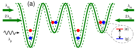
Illuminated by the modulated pumping laser, we consider cold AEA gases confined in an one-dimensional driven superlattice, which is illustrated intuitively in Fig.1(a). The pumping laser interrogates the transition between the ground states and the excited states . Such superlattice is formed by overlapping two 1D optical lattices with one at a magic wavelength giving lattice depth , and the other at the wavelength giving the depth and for the state and respectively. To simplify our discussion, the superlattice and pumping laser are assumed to be driven simultaneously and the sine protocol is chosen, which can be achieved by acousto-optic modulators.
Define and as the projection operator to the ground states and the excited states respectively, the driven state-dependent superlattice can be written as
| (1) | |||||
where the sinusoidal driven function is applied
| (2) |
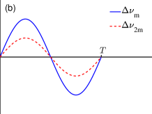
denotes the driving frequency. The right hand side of the first line in Eq.(1) indicates that the atomic two levels feel the same lattice potential generated by the magic wavelength . In contrast, the second and third lines describe different trapping conditions due to the laser with wavelength . Assuming identical spatial shaking for the two lattice, the two driven protocols should be coordinated as shown in Fig.1(b). Let be the frequency excursion of the modulation to the magic laser frequency. Such condition can be achieved by just choosing the frequency excursion for the other one.
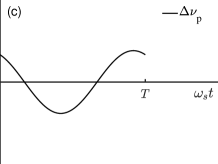
Considering another time-dependent modulation to the frequency of the pumping laser,
| (3) |
which is shown in Fig.1(c), the transition can be described by the atom-laser couping matrix(under the rotating-wave approximation),
with
| (4) |
Here is the Rabi frequency, is the detunning, is the frequency difference between and , and is the wavelength and wave number of pumping laser. It is noteworthy that we have introduced an initial phase difference between the two driven functions in Eq.(2), which is the key ingredient for engineering the periodic flux in our following discussions. According to cold AEA experiments such as 173YbMancini2015 ; Livi2016 and 87SrKolkowitz2017 ; Lu2021 ; Yin2022 , neglecting atomic interaction in some suitable lattices is reasonable. Under individual-particle approximation, then the external and internal motion of the atoms is governed by the Hamiltonian
| (5) |
where and are the atomic mass and momentum, is the identity operator associated with the internal atomic degrees of freedom.
III effective Hamiltonian and periodic gauge fields
It is convenient to work in the frame of reference co-moving with the superlattice, into which we can transform the atomic motion by two steps of unitary transformation. First, we define and transform the Hamiltonian in Eq.(5) by . The shift of position in the potential is compensated by . However, the extra term generates , which means a shift of the momentum. To cancel this extra term, we implement the other unitary transformation by , which results in . Finally, the Hamiltonian in the co-moving frame becomes
| (6) |
with the undriven superlattice potential
| (7) | |||||
Here the term can be ignored since it is a time-dependent energy shift. In this laboratory frame, we can see now that the vibration of superlattice gives rise to two physical effects. The first is the inertial force, given by , which generates the energy term . The second is the Doppler effect, related to the term .
In Wannier representation using the tight-binding approximation, the many-body Hamiltonian described by Eq.(III) can be formulated as
| (8) | |||||
where () and () denote the fermionic annihilation(creation) operator for atoms occupying the Wannier state at the a and b sublattice of the th site respectively, is the corresponding tunnelling amplitude, and , label the internal states , respectively. Here the phase that can be changed by adjusting the angle between the pumping laser and the superlatticeLivi2016 . The energies associated with the inertial force acting on atoms at different sites are given by
| (9) |
Let be the chemical potentials of atoms in superlattice. Then the corresponding total potentials should include the detuning related energy, namely . Since we are interested in Floquet photon assisted resonant processes, we set these potentials equal to integer multiples of ,
| (10) | |||||
where the minimum is redefined as the zero point of potential energy. This condition can be satisfied by choosing proper lattice laser power, pumping laser frequency and driving frequency.
We proceed to discuss the resonant situation. In this case, we need to combine the potentials with the inertial force induced energies and the Doppler effect associated terms in Eq(8). Based on this consideration, we do a combined rotation transformation of and , which leads to the new Hamiltonian
| (11) | |||||
where
| (12) |
with denoting or , and .
In a typical AEA experiment, for example 87Sr atomsLu2021 ; Yin2022 , the driving frequency can vary from several hundreds to several kilohertz, and the superlattice depth ranges from near zero to tens of recoil energies(the the recoil energy is defined as ). Therefore, we can adjust the experimental parameters to ensure that the driven frequency is larger than the inter-site tunneling amplitudes and the Rabi frequency, and then the high-frequency expansion can be applied safely. In our proposal, the periodical modulation is sin signal function, as shown in Eq.(2) and Eq.(3). We make use of the Bessel function expansion, , to replace the driven modulation terms in Eq.(III). Keeping only the resonant processes and neglecting other rapidly oscillating terms, the renormalized parameters of Eq.(III) can be approximately expressed as
| (13) |
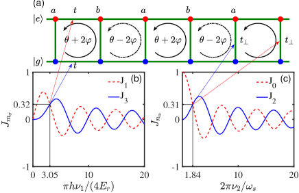
where and . Finally, substituting Eq.(III) into Eq.(11), we obtain a time-independent effective Hamiltonian. By employing internal atomic degrees of freedom as the extra lattice dimension, it can be regarded as a two-leg flux ladder model depicted in Fig.2(a).
From the last line in Eq.(III), we can see that phases , and thus the relevant gauge fields, emerge from the internal state resonant transition with the assistance of Floquet photons. As for this artificial gauge field, the physical gauge-invariant quantity is the phase accumulated on an elementary loop per plaquette. Taking into account the phase , the total magnetic flux through each plaquette is . One should note that for odd , which implies an additional phase. To simplify the analysis, we always choose and such that the total extra phases can be eliminated. Take a particular case of , , , as an example, the accumulated phase is . Now it is clear that our scheme can simulate the periodic gauge fields with two plaquette as one period. Recall that is induced by incommensurate ratio between wavelengths of the lattice and the pumping lasers, it can be tuned by adjusting the angle between those lasers. Moreover, is the initial phase of the sinusoidal driving function and is fully controllableLu2021 . Thus our scheme offers a feasible method to tune the periodic gauge potentials.
Finally, we discuss the modulation of hopping amplitudes in the effective model. The Bessel functions from Eq.(III) renormalize the nearest-neighbor hopping amplitudes along legs as and along rungs as , respectively. Independent of the phases , , such simple parameter-dependent function forms result in their individual controllability via varying the driving amplitudes , . While the demonstrated controllability offers exciting possibilities, it is essential to first consider the widely studied cases with equal hopping amplitudes along legs and along rungs. Fig.2(b) shows the Bessel functions for and . The crossing points indicate the equal tunneling amplitudes along legs if considering . Similarly, Fig.2(c) illustrates the tuned hopping amplitudes across rungs, with equal points clearly visible.
IV Topological phase
Now we investigate topological phase of the ladder model caused by the gauge fields. For clarity, we rewrite the effective Hamiltonian for the case of , , , ,
| (14) | |||||
where , , , and the proper gauge transformation is preformed. When , namely the uniform flux scenario, previous research has demonstrated that no topological states are present in this 1D systemHugel2014 . When and , recent work by Zhao’s group shows that nontrivial topological states manifest, and the topological invariant can be entirely determined by the projective symmetry algebraJiang2024 . For being the rational number, SunSun2016 has studied the particular case of periodic fluxes with period three, , , , where the 1D topological invariant was elucidated with the help of the Chern numbers of the corresponding extended 2D system.
To explore the effects of general periodic gauge fields in Eq.(14), we notice that this model exhibits combined symmetry of inversion and time-reversal :
| (15) |
In momentum space, the Hamiltonian and operator are respectively represented by
| (16) |
where , denote Pauli matrices and the complex conjugation. Since , the operator can be transformed into by a unitary transformation, and the corresponding Hamiltonian will be required to be real in this basis. When the number of ouccpied bands is one or three, the ground state is classified by the first Stiefel-Whitney class and characterized by a -valued topological invariant Ahn2018 ; Fang2015 . The topological invariant can be formulated with the help of the Wilson loop. Introducing the nonabelian gauge connection , where , are the wave functions of occupied bands, then the Wilson loop is constructed as
| (17) |
where indicate path ordering. is defined by the determinate of ,
| (18) |
where are eigenvalues of . Due to the symmetry, can only take value 0 or Ahn2018 .
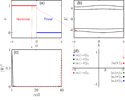
Taking 87Sr atoms as an example, can be approximated as if the pumping laser is parallel to the lattice laserKolkowitz2017 ; Yin2022 . We set as 4, and restrict within the interval because of its periodicity. Applying invariant formulas in Eq.(17) and Eq.(IV) to the lowest filled band of the Hamiltonian in Eq.(IV), one finds that for and is trivial otherwise, as shown in Fig.3(a). The topological number can be explained as followsAhn2018 . Considering the lowest band of energy spectrum[see Fig.3(b)], if we impose real conditions on the bulk wave function over the Brillouin zone, the wave function can be made smooth over , and glued on the boundaries but with an orientation-reversing transition function. The transition function equaling to one indicates that the state is orientable and , while minus one indicates that the state is non-orientable and , as intuitively depicted in Fig.3(d). Fig.3(c) shows the probability of a pair of edge states located inside the energy gap separating the second band form the lowest one, calculated for 40 unit cells with open boundary conditions when . When , the system simplifies to the case of uniform fluxes, and the number of sites per unit cell reduces from four to two. This reduction indicates that the energy gap should close when , which corresponds to a topological phase transition.
Additionally, we note that a similar discussion of topological properties can be conducted for three occupied bands, yielding the same results as that for one occupied bands.
V Conclusions
In conclusion, we present a simple and feasible proposal for engineering a two-leg ladder model with periodic gauge fields based on driven cold AEA optical lattice systems. The periodic gauge field is widely controllable by independently changing the parameters of the driven protocol. Our proposal can simulate real topological phase described by the first Stiefel-Whitney class, and demonstrate topological phase transition induced by gauge fields. Our scheme utilizes the long-lived electronic internal state, and thus offers a highly promising candidate for future experimental implementation and observation. We hope these features of this work could enrich the gauge field-related topological research both in theory and in experiments.
Recently, the time-dependent synthetic gauge potentials has been theoretically confirmed as the critical ingredient for realizing tailored dynamical evolution of quasiparticles, quasiholesWang2018 ; Raciunas2018 ; Wang2022 , wave packetsYilmaz2018 ; Lelas2021 , as well as adiabatic state preparationWang2021 . Another application of our proposal is expected for those dynamical process studies.
Acknowledgements
This work was supported by the National Science Foundation of China under Grant No. 12274045. T. Wang acknowledges funding from the National Science Foundation of China under Grants No.12347101 and funding from the Program of State Key Laboratory of Quantum Optics and Qauntum Optics Devices (Grant No. KF202211).
References
- (1) K. V. Klitzing, G. Dorda, and M. Pepper, Phys. Rev. Lett. 45, 494 (1980).
- (2) R. B. Laughlin, Phys. Rev. B 23, 5632 (1981).
- (3) D. J. Thouless, M. Kohmoto, M. P. Nightingale, and M. Dennijs, Phys. Rev. Lett. 49, 405 (1982).
- (4) D. C. Tsui, H. L. Stormer, and A. C. Gossard, Phys. Rev. Lett. 48, 1559 (1982).
- (5) R. B. Laughlin, Phys. Rev. Lett. 50, 1395 (1983).
- (6) M. Z. Hasan and C. L. Kane, Rev. Mod. Phys. 82, 3045 (2010).
- (7) X. L. Qi and S. C. Zhang, Rev. Mod. Phys. 83, 1057 (2011).
- (8) C. K. Chiu, J. C. Y. Teo, A. P. Schnyder, and S. Ryu, Rev. Mod. Phys. 88, 035005 (2016).
- (9) A. Bansil, H. Lin, and T. Das, Rev. Mod. Phys. 88, 021004 (2016).
- (10) N. P. Armitage, E. J. Mele, and A. Vishwanath, Rev. Mod. Phys. 90, 015001 (2018).
- (11) F. D. M. Haldane, Phys. Rev. Lett. 61, 2015 (1988).
- (12) K. Ohgushi, S. Murakami, and N. Nagaosa, Phys. Rev. B. 62, R6065 (2000).
- (13) K. Sun, Z. C. Gu, H. Katsura, and S. Das Sarma, Phys. Rev. Lett. 106, 236803 (2011).
- (14) T. Neupert, L. Santos, C. Chamon, and C. Mudry, Phys. Rev. Lett. 106, 236804 (2011).
- (15) W. C. Chen, R. Liu, Y. F. Wang, and C. D. Gong, Phys. Rev. B. 86, 085311 (2012).
- (16) R. C. Ge and M. Kolodrubetz, Phys. Rev. B 104, 035427 (2021).
- (17) D. H. Guan, L. Qi, X. Y. Zhang, Y. J. Liu, and A. L. He, Phys. Rev. B 108, 085121 (2023).
- (18) Z. Y. Lan, A. L. He, and Y. F. Wang, Phys. Rev. B 107, 235116 (2023).
- (19) G. Xu, B. Lian, and S. C. Zhang, Phys Rev Lett 115, 186802 (2015).
- (20) S. J. Zhang, C. W. Zhang, S. F. Zhang, W. X. Ji, P. Li, P. J. Wang, S. S. Li, and S. S. Yan, Phys. Rev. B 96, 205433 (2017).
- (21) A. L. He, W. W. Luo, Y. Zhou, Y. F. Wang, and H. Yao, Phys. Rev. B 105, 235139 (2022).
- (22) A. L. He, X. Y. Zhang, and Y. J. Liu, Phys. Rev. B 106, 125147 (2022).
- (23) R. Liu, W. C. Chen, Y. F. Wang, and C. D. Gong, J. Phys.-Condens. Mat. 24, 305602 (2012).
- (24) Y. F. Wang and C. D. Gong, Phys. Rev. Lett. 98, 096802 (2007).
- (25) G. Y. Sun, Phys. Rev. A 93, 023608 (2016).
- (26) H. Cai, J. H. Liu, J. Z. Wu, Y. Y. He, S. Y. Zhu, J. X. Zhang, and D. W. Wang, Phys. Rev. Lett. 122, 023601 (2019)
- (27) Y. X. Zhao, Y. X. Huang, and S. Y. A. Yang, Phys. Rev. B 102, 161117 (2020).
- (28) L. B. Shao, Q. Liu, R. Xiao, S. Y. A. Yang, and Y. X. Zhao, Phys. Rev. Lett. 127, 076401 (2021).
- (29) Z. Y. Chen, S. Y. A. Yang, and Y. X. Zhao, Nat. Commun. 13, 1038 (2022).
- (30) Z. Y. Chen, Z. Zhang, S. Y. A. Yang, and Y. X. Zhao, Nat. Commun. 14, 1038 (2023).
- (31) C. Zhang, Z. Y. Chen, Z. Zhang, and Y. X. Zhao, Phys. Rev. Lett. 130, 256601 (2023).
- (32) G. Jiang, Z. Chen, S. Yue, W. Rui, X.-M. Zhu, S. A. Yang, and Y. Zhao, Phy. Rev. B 109, 115155 (2024).
- (33) Y. X. Zhao, C. Chen, X. L. Sheng, and S. Y. A. Yang, Phys. Rev. Lett. 126, 196402 (2021).
- (34) H. R. Xue, Z. H. Wang, Y. X. Huang, Z. Y. Cheng, L. T. Yu, Y. X. Foo, Y. X. Zhao, S. Y. A. Yang, and B. L. Zhang, Phys. Rev. Lett. 128, 116802 (2022).
- (35) H. R. Xue, Z. Y. Chen, Z. Y. Cheng, J. X. Dai, Y. Long, Y. X. Zhao, and B. L. Zhang, Nat. Commun. 14, 1038 (2023).
- (36) J. Dalibard, F. Gerbier, G. Juzeliūnas, and P. Öhberg, Rev. Mod. Phys. 83, 1523 (2011).
- (37) N. Goldman, G. Juzeliūnas, P. Öhberg, and I. B. Spielman, Rep. Prog. Phys. 77, 126401 (2014).
- (38) S. L. Zhang and Q. Zhou, J. Phys. B: At. Mol. Opt. Phys. 50, 222001 (2017).
- (39) M. Aidelsburger, J. Phys. B: At. Mol. Opt. Phys. 51, 193001 (2018).
- (40) C. Weitenberg and J. Simonet, Nat. Phys. 17, 1342 (2021).
- (41) M. R. Matthews, B. P. Anderson, P. C. Haljan, D. S. Hall, C. E. Wieman, and E. A. Cornell, Phys. Rev. Lett. 83, 2498 (1999).
- (42) K. W. Madison, F. Chevy, W. Wohlleben, and J. Dalibard, Phys. Rev. Lett. 84, 806 (2000).
- (43) J. R. Abo-Shaeer, C. Raman, J. M. Vogels, and W. Ketterle, Science 292, 476 (2001).
- (44) P. Engels, I. Coddington, P. C. Haljan, V. Schweikhard, and E. A. Cornell, Phys. Rev. Lett. 90, 170405 (2003).
- (45) V. Schweikhard, I. Coddington, P. Engels, V. P. Mogendorff, and E. A. Cornell, Phys. Rev. Lett. 92, 040404 (2004).
- (46) J. Ruostekoski, G. V. Dunne, and J. Javanainen, Phys. Rev. Lett. 88, 180401 (2002).
- (47) D. Jaksch and P. Zoller, New J. Phys. 5, 56 (2003).
- (48) W. Yi, A. J. Daley, G. Pupillo, and P. Zoller, New J. Phys. 10, 073015 (2008).
- (49) F. Gerbier and J. Dalibard, New J. Phys. 12, 033007 (2010).
- (50) A. Celi, P. Massignan, J. Ruseckas, N. Goldman, I. B. Spielman, G. Juzeliūnas, and M. Lewenstein, Phys. Rev. Lett. 112, 043001 (2014).
- (51) M. Aidelsburger, M. Atala, S. Nascimbene, S. Trotzky, Y. A. Chen, and I. Bloch, Phys. Rev. Lett. 107, 255301 (2011).
- (52) A. Eckardt, C. Weiss, and M. Holthaus, Phys. Rev. Lett. 95, 260404 (2005).
- (53) H. Lignier, C. Sias, D. Ciampini, Y. Singh, A. Zenesini, O. Morsch, and E. Arimondo, Phys. Rev. Lett. 99, 220403 (2007).
- (54) A. Zenesini, H. Lignier, D. Ciampini, O. Morsch, and E. Arimondo, Phys. Rev. Lett. 102, 100403 (2009).
- (55) J. Struck, C. Olschlager, R. Le Targat, P. Soltan-Panahi, A. Eckardt, M. Lewenstein, P. Windpassinger, and K. Sengstock, Science 333, 996 (2011).
- (56) P. Hauke, O. Tieleman, A. Celi, C. Olschlager, J. Simonet, J. Struck, M. Weinberg, P. Windpassinger, K. Sengstock, M. Lewenstein, and A. Eckardt, Phys. Rev. Lett. 109, 145301 (2012).
- (57) K. Jimenez-Garcia, L. J. LeBlanc, R. A. Williams, M. C. Beeler, A. R. Perry, and I. B. Spielman, Phys. Rev. Lett. 108, 225303 (2012).
- (58) N. Goldman and J. Dalibard, Phys. Rev. X 4, 031027 (2014).
- (59) M. Bukov, M. Kolodrubetz, and A. Polkovnikov, Phys. Rev. Lett. 116, 125301 (2016).
- (60) K. Plekhanov, G. Roux, and K. Le Hur, Phys. Rev. B 95, 045102 (2017).
- (61) J. Struck, C. Olschlager, M. Weinberg, P. Hauke, J. Simonet, A. Eckardt, M. Lewenstein, K. Sengstock, and P. Windpassinger, Phys. Rev. Lett. 108, 225304, 225304 (2012).
- (62) A. Eckardt, Rev. Mod. Phys. 89, 011004 (2017).
- (63) J. Struck, M. Weinberg, C. Olschlager, P. Windpassinger, J. Simonet, K. Sengstock, R. Hoppner, P. Hauke, A. Eckardt, M. Lewenstein, and L. Mathey, Nat. Phys. 9, 738 (2013).
- (64) G. Jotzu, M. Messer, R. Desbuquois, M. Lebrat, T. Uehlinger, D. Greif, and T. Esslinger, Nature 515, 237 (2014).
- (65) N. Flaschner, B. S. Rem, M. Tarnowski, D. Vogel, D. S. Luhmann, K. Sengstock, and C. Weitenberg, Science 352, 1091 (2016).
- (66) B. T. Wang, F. N. Unal, and A. Eckardt, Phys. Rev. Lett. 120, 243602 (2018).
- (67) M. Mancini, G. Pagano, G. Cappellini, L. Livi, M. Rider, J. Catani, C. Sias, P. Zoller, M. Inguscio, M. Dalmonte, and L. Fallani, Science 349, 1510 (2015).
- (68) M. L. Wall, A. P. Koller, S. M. Li, X. B. Zhang, N. R. Cooper, J. Ye, and A. M. Rey, Phys. Rev. Lett. 116, 035301 (2016).
- (69) L. F. Livi, G. Cappellini, M. Diem, L. Franchi, C. Clivati, M. Frittelli, F. Levi, D. Calonico, J. Catani, M. Inguscio, and L. Fallani, Phys. Rev. Lett. 117, 220401 (2016).
- (70) S. Kolkowitz, S. L. Bromley, T. Bothwell, M. L. Wall, G. E. Marti, A. P. Koller, X. Zhang, A. M. Rey, and J. Ye, Nature 542, 66 (2017).
- (71) S. L. Bromley, S. Kolkowitz, T. Bothwell, D. Kedar, A. Safavi-Naini, M. L. Wall, C. Salomon, A. M. Rey, and J. Ye, Nat. Phys. 14, 399 (2018).
- (72) X. T. Lu, T. Wang, T. Li, C. H. Zhou, M. J. Yin, Y. B. Wang, X. F. Zhang, and H. Chang, Phys. Rev. Lett. 127, 033601 (2021).
- (73) M. J. Yin, X. T. Lu, T. Li, J. J. Xia, T. Wang, X. F. Zhang, and H. Chang, Phys. Rev. Lett. 128, 073603 (2022).
- (74) D. Hügel and B. Paredes, Phys. Rev. A 89, 023619 (2014).
- (75) C. Fang, Y. G. Chen, H. Y. Kee, and L. Fu, Phys. Rev. B 92, 081201 (2015).
- (76) J. Ahn, D. Kim, Y. Kim, and B. J. Yang, Phys. Rev. Lett. 121, 106403 (2018).
- (77) M. Raciunas, F. N. Unal, E. Anisimovas, and A. Eckardt, Phys. Rev. A 98, 063621 (2018).
- (78) B. T. Wang, X. Y. Dong, and A. Eckardt, SciPost Phys. 12, 095 (2022).
- (79) F. Yilmaz and M. O. Oktel, Phys. Rev. A 97, 023612 (2018).
- (80) K. Lelas, O. Celan, D. Prelogovic, H. Buljan, and D. Jukic, Phys. Rev. A 103, 013309 (2021).
- (81) B. T. Wang, X. Y. Dong, F. N. Unal, and A. Eckardt, New J. Phys. 23, 063017 (2021).