Deciding factor for detecting a particle within a subspace via dark and bright states

Abstract

In a measurement-induced continuous-time quantum walk, we address the problem of detecting a particle in a subspace, instead of a fixed position. In this configuration, we develop an approach of bright and dark states based on the unit and vanishing detection probability respectively for a particle-detection in the subspace. Specifically, by employing the rank-nullity theorem, we determine several properties of dark and bright states in terms of energy spectrum of the Hamiltonian used for a quantum walk and the projectors applied to detect the subspace. We provide certain conditions on the position and the rank of the subspace to be detected, resulting in the unit total detection probability, which has broad implications for quantum computing. Further, we illustrate the forms of dark as well as bright states and the dependence of detection probability on the number of dark states by considering a cyclic graph with nearest-neighbor and next nearest-neighbor hopping. Moreover, we observe that the divergence in the average number of measurements for detecting a particle successfully in a subspace can be reduced by performing high rank projectors.

I Introduction

The quantum mechanical analogue of a classical random walk, referred to as quantum walk kempe2003rev; andraca2012; Kadian2021, can be classified into two distinct categories – discrete-time and continuous-time quantum walk. Due to the quantum superposition principle, quantum walk represents a sophisticated framework for constructing quantum algorithms which, in turn, results in a universal paradigm for quantum computation Karafyllidis2005; childs2009; lovett2010; Kendon2014; Singh2021. In particular, it has been utilized in a wide range of quantum information processing tasks, including quantum search shenvi2003; Wong2015; Li2020, quantum encryption and security Rohde2012; el-latif2020, cryptographic systems Abd-El-Atty2021, random number generation bae2021; bae2022, state engineering vieira2013; innocenti2017; giordani2019; Kadian2021 to name a few. Additionally, quantum walks have been experimentally implemented Manouchehri2014 using nuclear magnetic resonance du2003; ryan2005, photonic perets2008; bian2017 and optomechanical systems Moqadam2015, and trapped ions Karski2009.

One of the primary objectives of continuous-time quantum walks is to determine the probability and time of arriving at a certain location when a particle starts from a particular initial position. Despite controversies surrounding the consideration of time as an operator mielnik2011time, significant progress have been achieved when addressing the time-of-arrival problem in the literature Allcock1969; Kijowski1974; Halliwell2009; Anastopoulos2006; Aharonov1998; Kumar1985; Galapon2012; Galapon2004; Galapon2005; Chakraborty2016. Concurrently, several quantum search setups Grover1997; Childs2004; Magniez2011; Novo2015; Li2017 have been proposed, in conjunction with investigations into state transfer phenomena tanner2009; bohm2015. In addition to the approaches, a periodic measurement strategy combined with unitary evolution – which is determined by the Hamiltonian of a certain system – can be employed to identify the particle. Within this realm, the measurement process dynamically influences the evolution of the state of the walker.

In stroboscopic measurement-induced quantum walk (MIQW) Didi2022, the first-detected arrival problem becomes relevant Krovi2006hitting; krovi2006hypercube; Krovi2007quotient over the first arrival time, which excludes stroboscopic measurements. Specifically, determining the walker in the target state using periodic measurements for the first time after beginning from some initial state is known as the first detection problem. While measurements impede the quantum walker’s free evolution, this problem has attracted a lot of attention Sinkovicz2016; Sinkovicz2015; Dhar2015; Grunbaum-schur-func2014; Caruso2009 since it is related to readout techniques in quantum computing tasks and control of quantum systems butkovskiy1990control; Huang1983; Pierce1988; rabitz2000; Wiseman_Milburn_2009; campo2015. Moreover, MIQW is intricately linked to mid-circuit measurements Govia2023; norcia2023; norcia2023yb, a key component in quantum computing, error correction hashim2024quasiprobabilistic and mitigation botelho2022 and has also been implemented on IBM quantum computers equipped with a mid-circuit readout feature wang2024hitting. From a more fundamental perspective, this method of detecting a particle in a fixed position may further highlight the role of measurements in quantum theory Li2019; muller2022; feng2023; poboiko2024.

The total probability of the first detection, referred to as the total detection probability, is the statistics of the walker’s detection for the first time during the application of an infinite number of stroboscopic measurements in MIQW Krovi2006hitting; krovi2006hypercube; Krovi2007quotient; FriedmanKessler2017; Allcock1969; Galapon2004; Galapon2005; Kumar1985; Aharonov1998; Anastopoulos2006; Allcock1969. To emphasize, there exist certain initial conditions under which the desired state is never achieved due to destructive interference in the system; we refer to these states as dark states plenio1998; Barkai2020DarkState in accordance with forbidden transitions in atomic physics, whereas bright states can be recognized with certainty. It has been shown that the probability of identifying these states is connected with the existence of dark and bright energy states in the system Barkai2020DarkState; Liu2022.

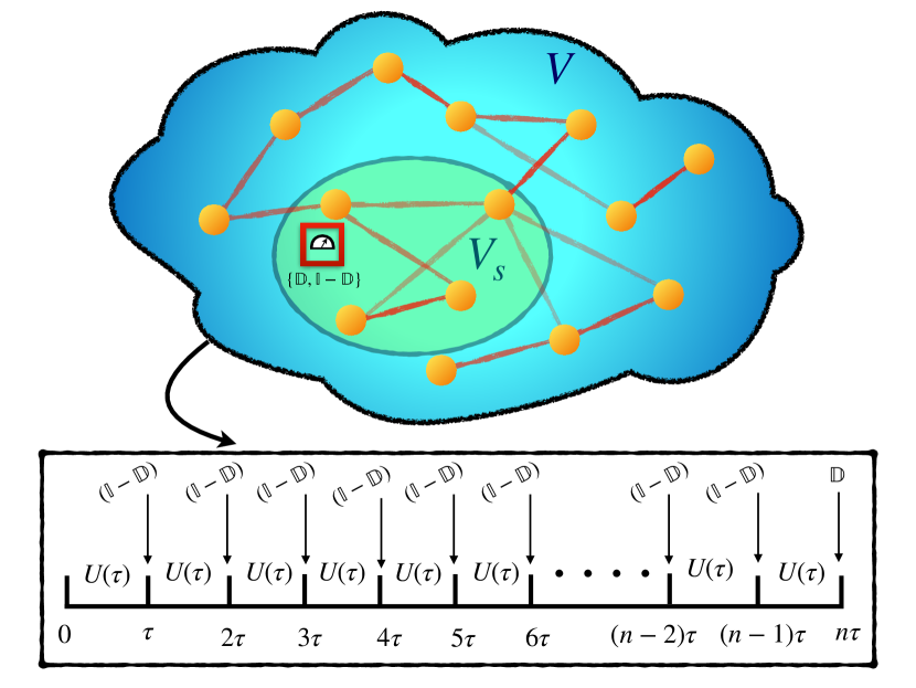
Figure 1: Schematic diagram of first detection of the walker in subspace $V_{s}$ of a finite graph, consisting of a set of vertices $V$ with measurement-induced quantum walk. In the MIQW protocol, the first hitting time statistics $F_{n}$ is captured through the application of unitary dynamics, $U(\tau)$, punctuated intermittently by measurements $\{\mathbb{D},\mathbb{I-D}\}$ taken in a stroboscopic fashion with time interval $\tau$. Here, the $\mathbb{D}$ is the detector corresponding to the subspace $V_{s}$. The schematic shows that upto $(n-1)$th round of measurements, no-click event is occurring, i.e., the subspace $V_{s}$ is not detected, while after the $n$th round of measurement, the particle is detected in subspace $V_{s}$ which corresponds to a successful click event. After successful detection the protocol is stopped.

We employ the concepts of dark and bright energy levels to address the problem of detecting a particle in a subspace (see Fig. 1 for schematics), going beyond locating it in a single site. It has also been addressed by using different methods, namely non-Hermitian approach Dhar2015 and by establishing its connection with the properties of Schur function Grunbaum-schur-func2014. It is crucial to highlight that in certain cases, the method proposed here can explain the total detection probability in a more simpler manner than the existing methods. In this work, we adopt the rank-nullity theorem golub2013matrix to establish a connection between the existence of dark and bright states by selecting a subspace from the set of vertices of a discrete, and finite graph in which the particle has to be identified. In contrast to the scenario encountered in a localized single-site detection within a graph, we exhibit that for each degenerate energy level, there can exist more than one bright energy state, in the subspace detection within a system. Subsequently, we derive explicit formulae for the orthonormal states within the dark energy subspace and its corresponding complementary bright energy subspace. We demonstrate that the total detection probability decreases monotonically with an increase in the number of dark states in the system which is related to the increase of rank and the position of the detector. Importantly, we provide a necessary and sufficient condition for detecting a particle in a subspace with certainty in an arbitrary finite graph having discrete, bounded and degenerate spectrum independent of vertex-localized initial states which can be important in quantum computation. We observe that increasing the rank of the subspace and strategically placing detectors can minimize the divergences in average hitting time observed in the case of a single-site detection.

The paper is organized in the following manner. In Sec. II, the problem of subspace detection and the quantities of interest are discussed. In the context of a particle to be detected in a subspace, the notion of dark as well as bright states and the criteria for unit detection probability are presented in Sec. III. Sec. IV illustrates another method for computing the total detection probability based on the computation of matrices numerically while both the methods are applied on interacting systems with nearest-neighbor and next nearest-neighbor hopping in Sec. V. In Sec. LABEL:sec:avnomeasure, we study the pattern of the average number of measurement in detecting a particle in subspace while the results are summarized in Sec. LABEL:sec:conclu.

II Stroboscopic subspace detection protocol

Let us consider a quantum mechanical particle moving on a finite graph having a set of vertices $V$$=\left\{\ket{l}\Big{|}\sum_{l=1}^{L}\outerproduct{l}{l}=\mathbb{I}\text{ and }\innerproduct{l}{m}=\delta_{l,m}\right\}_{l=1}^{L}$, described by a time-independent Hamiltonian $H=-\sum_{l,m=1}^{L}\gamma_{lm}\outerproduct{l}{m}$ where $\gamma_{lm}$ are constants. Thus, unitary dynamics of the initial state, $\ket{\phi(0)}$, leads to the evolved state at time, $t$, as $\ket{\phi(t)}=U(t)\ket{\phi(0)}=e^{-iHt}\ket{\phi(0)}$. In the context of hitting problem Krovi2006hitting; Varbanov2008 in MIQW, we are interested to determine the position of particle in a given subspace of $V$. Towards achieving the same, we perform repeated projective measurements with periodicity $\tau$, corresponding to the subspace $V_{s}=\{\ket{d_{i}}\}_{i=1}^{\tilde{r}<L}$, written as

$$\bigg{\{}\mathbb{D}=\sum_{i=1}^{\tilde{r}<L}\outerproduct{d_{i}}{d_{i}},\mathbb{I}-\mathbb{D}\bigg{\}},$$ (1)

where $\ket{d_{i}}$ can be any vertex of $V$ with $\innerproduct{d_{i}}{d_{j}}=\delta_{i,j}$ and $\tilde{r}$ represents the rank of the detector, $\mathbb{D}$. Under the assumption that the measurements are performed instantaneously, we consider a sequence of measurements until the particle is detected. Therefore, if the particle remains undetected up to $(n-1)$ number of measurement rounds, the unnormalized resulting state just before the successful detection at round $n$ can be written as

$$\ket{\phi(n\tau)}\equiv\ket{\phi(n)}=U(\tau)[(\mathbb{I}-\mathbb{D})U(\tau)]^{n-1}\ket{\phi(0)}.$$ (2)

The first detection probability, i.e., the probability in detecting the particle for the first time after $n$th measurement attempt is given by Dhar2015; FriedmanKessler2017

$$F_{n}=\bra{\phi(n)}\mathbb{D}\ket{\phi(n)},$$ (3)

while the total first detection probability, $P_{\det}$ of the particle is defined as the detection probability after an infinite number of measurements conditioned on the fact that once the particle is detected, measurement process is stopped Barkai2020DarkState; FriedmanKessler2017. Alternatively, we call it as total detection probability, and mathematically, we can write it as

$$P_{\det}=\sum_{n=1}^{\infty}F_{n}.$$ (4)

Also, the probability of the particle surviving the first $n$ rounds of measurement can be written as

$$S_{n} = 1-\sum_{k=1}^{n}F_{k}$$ (5)

$$= \bra{\phi(n)}(\mathbb{I-D})\ket{\phi(n)}$$

$$= \bra{\phi(0)}[U^{\dagger}(\tau)(\mathbb{I-D})]^{n}[(\mathbb{I-D})U(\tau)]^{n}\ket{\phi(0)}$$

$$= \bra{\phi(0)}\mathbb{S}^{{\dagger}^{n}}\mathbb{S}^{n}\ket{\phi(0)},$$

where $\mathbb{S}\equiv(\mathbb{I}-\mathbb{D})U(\tau)$ is the survival operator. Therefore, the final survival probability (i.e., in $\lim_{n\to\infty}S_{n}$) reads as

$$P_{\operatorname{\text{sur}}}=\lim_{n\to\infty}S_{n}=1-P_{\det}.$$ (6)

In the case of identifying a particle in a fixed subspace, we will be focusing on developing a framework that can be utilized to obtain total detection probability.

III Prescription for calculation of total detection probability through dark and bright energy subspace

We now develop a method that leads to a definite conclusion about whether a particle resides in a given region. In particular, we investigate the trends of the total detection probability, $P_{\det}$, by varying the subspace in which the particle is to be detected. To address this question, we provide a framework aimed at partitioning the energy space of the Hamiltonian into two distinct orthogonal subspaces, namely dark and bright subspaces Barkai2020DarkState.

Dark and bright states. Given an initial state $\ket{\phi(0)}$, $P_{\det}(\phi(0))=0$, i.e., $F_{n}=0\forall n$ represents a dark state with respect to a detection space $\mathbb{D}$ on the other hand, $P_{\det}(\phi(0))=1$ corresponds to bright state which is detected with certainty. However, there can be initial states that are neither completely dark nor bright, and the first detection probability lies between $0$ and $1$, i.e., $0<P_{\det}<1$.

We are interested in the stationary dark states, which are the eigenstates of both the unitary evolution $U(\tau)$ and survival operator $\mathbb{S}$. Let us denote the $k$-th energy level of the Hamiltonian, $H$ as $E_{k}$ and the corresponding set of eigenvectors as $\{\ket{E_{k,m}}\}_{m=1}^{g_{k}}$ where $g_{k}$ is the degeneracy of $E_{k}$. If an energy level is non-degenerate, we omit the index $m$. We consider two different scenarios in case of degeneracy of $E_{k}$ while finding conditions for dark state to exist.

(i) Non-degenerate energy levels. According to the definition, a non-degenerate energy level $E_{k}$ is a dark state if

$$\mathbb{D}\ket{E_{k}}=0,$$ (7)

and

$$(\mathbb{I}-\mathbb{D})U(\tau)\ket{E_{k}}=\exp(-iE_{k}\tau)\ket{E_{k}}.$$ (8)

The condition in Eq. (7) for a non-degenerate energy eigenstate to be a dark state can be equivalently expressed as $\innerproduct{d_{i}}{E_{k}}=0$ $\forall i$. In the other scenario, i.e., for degenerate energy levels, the physics of dark and bright states with respect to subspace detection is much more captivating as discussed below.

(ii) Degenerate energy levels. In case of degenerate eigenstates, $\{\ket{E_{k,m}}\}_{m=1}^{g_{k}}$, we construct an projector $\mathbb{E}_{k}$ which can be written mathematically as

$$\mathbb{E}_{k}=\sum_{m=1}^{g_{k}}\outerproduct{E_{k,m}}{E_{k,m}}.$$ (9)

Here, the first index $k$ in $\ket{E_{k,m}}$ corresponds to the distinct energy level, and the second index $m$ indicates the level of degeneracy present in each level. To find out the existence of dark states in the corresponding degenerate subspace, let us write any dark state in that particular subspace as

$$\ket{\zeta_{k}}=\sum_{m=1}^{g_{k}}\alpha_{m}\ket{E_{k,m}}.$$ (10)

Therefore, by Eq. (7) we get

$$\mathbb{D}\ket{\zeta_{k}} = 0$$ (11)

$$\implies\sum_{i=1,m=1}^{\tilde{r},g_{k}}\alpha_{m}\ket{d_{i}}\innerproduct{d_{i}}{E_{k,m}} = 0,$$

$$\implies\sum_{m=1}^{g_{k}}\alpha_{m}\ket{d_{i}}\innerproduct{d_{i}}{E_{k,m}} = 0\forall i$$

$$\implies\mathcal{A}_{k}\ket{\tilde{\alpha}} = 0,$$ (12)

with the $\tilde{r}\times g_{k}$ matrix, $\mathcal{A}_{k}$, being

$$\mathcal{A}_{k}=\begin{bmatrix}\innerproduct{d_{1}}{E_{k,1}}&\innerproduct{d_{1}}{E_{k,2}}&\ldots&\innerproduct{d_{1}}{E_{k,g_{k}}}\\ \innerproduct{d_{2}}{E_{k,1}}&\innerproduct{d_{2}}{E_{k,2}}&\ldots&\innerproduct{d_{2}}{E_{k,g_{k}}}\\ \vdots&\vdots&\ddots&\vdots\\ \innerproduct{d_{r}}{E_{k,1}}&\innerproduct{d_{r}}{E_{k,2}}&\ldots&\innerproduct{d_{r}}{E_{k,g_{k}}}\\ \end{bmatrix},$$ (13)

and $\ket{\tilde{\alpha}}=(\alpha_{1},\alpha_{2},\ldots,\alpha_{g_{k}})^{T}$ being the coefficient vector of the dark state (see Eq. (10)). The above condition clearly shows that the existence of $\ket{\zeta_{k}}$ depends on the overlaps of $\ket{E_{k,m}}$ with $\ket{d_{i}}$, i.e, $\innerproduct{d_{i}}{E_{k,m}}$ $\forall i,m$. Let us proceed to analyze this matter through a systematic examination of individual cases.

Case I. Consider the scenario when $\innerproduct{d_{i}}{E_{k,m}}=0\text{ }\forall\text{ }i,m$. In this case, all the degenerate energy eigenstates $\{\ket{E_{k,m}}\}_{m=1}^{g_{k}}$ corresponding to energy $E_{k}$ are the dark states, i.e., $\ket{\zeta_{k}^{j}}=\ket{E_{k,j}}$ for $j=1,2,\ldots,g_{k}$. Therefore, the entire energy subspace is dark.

Case II. Let us consider a situation when $\innerproduct{d_{i}}{E_{k,m}}=0$ for some of $i$ and $m$ but not all of them. We present one of our main findings as Proposition 1, from which the number of dark states can be calculated. Note that in the complementary subspace to the dark subspace, the energy states are eventually bright states which will be proved later in Proposition 2.

Proposition 1.

Number of dark states in the subspace $\{\ket{E_{k,m}}\}_{m=1}^{g_{k}}$ is equal to the dimension of the null space of $\mathcal{A}_{k}$, denoted as $\dim({\mathcal{N_{A}}_{k}})$ while the number of bright states is equal to the rank of matrix $\mathcal{A}_{k}$, $\rank(\mathcal{A}_{k})$.

Proof.

It is evident from Eq. (12) that the existence of dark states is equivalent to finding non-trivial solutions $(\text{trivial solution is }\alpha_{i}=0\text{ for }i=1,2,\ldots,g_{k})$ of the matrix $\mathcal{A}_{k}$ which, in turn, is linked to the determination of its nullspace, denoted as $\mathcal{N}_{\mathcal{A}_{k}}$. Therefore, the number of dark states in the corresponding energy subspace is equal to dimension of the nullspace, i.e., $\dim{(\mathcal{N}_{\mathcal{A}_{k}})}$. Moreover, from rank-nullity theorem golub2013matrix, we know

$$\rank(\mathcal{A}_{k})+\dim(\mathcal{N_{A}}_{k})=\text{Number of columns of $\mathcal{A}_{k}$}=g_{k}.$$

(14)

Therefore, the number of bright states is just $\rank(\mathcal{A}_{k})$ since any degenerate subspace is spanned by dark states and its complement space, containing only bright states Barkai2020DarkState. Mathematically, we can write that $\{\ket{E_{k,m}}\}_{m=1}^{g_{k}}$ is spanned by $\left\{\left\{\ket{\zeta_{k}^{j}}\right\}_{j=1}^{\dim({\mathcal{N_{A}}_{k}})},\left\{\ket{\eta_{k}^{j}}\right\}_{j=1}^{\rank({\mathcal{A}_{k}})}\right\}$, i.e., following Eq. (9), it can be expressed as

$$\mathbb{E}_{k}=\sum_{j=1}^{\dim(\mathcal{N_{A}}_{k})}\outerproduct{\zeta_{k}^{j}}{\zeta_{k}^{j}}+\sum_{j=1}^{\rank(\mathcal{N_{A}}_{k})}\outerproduct{\eta_{k}^{j}}{\eta_{k}^{j}}.$$ (15)

∎

Let us now explicitly calculate the basis states consisting of bright and dark states for degenerate energy levels. The general form of the matrix $\mathcal{A}_{k}$ after performing row reduction on it and removing zero rows can be updated as

$$\mathcal{A}_{k}=\begin{bmatrix}a_{1,1}&a_{1,2}&\ldots&a_{1,l_{k}}&\ldots&a_{1,g_{k}}\\ 0&a_{2,2}&\ldots&a_{2,l_{k}}&\ldots&a_{2,g_{k}}\\ \vdots&\vdots&\ddots&\vdots&\vdots\\ 0&0&\ldots&a_{l_{k},l_{k}}&\ldots&a_{l_{k},g_{k}}\end{bmatrix}_{l_{k}\times g_{k}},$$ (16)

of reduced dimension where $l_{k}=\rank(\mathcal{A}_{k})\leq g_{k}$ with $a_{i,j}=0$ $\forall i>j$. Also from rank-nullity theorem, we know that the dark subspace corresponding to a degenerate energy $E_{k}$ exists if $l_{k}<g_{k}$. Now we can write one of the dark states as

$$\ket{\zeta_{k}^{1}}=N_{1}\begin{vmatrix}\ket{E_{k,1}}&\ket{E_{k,2}}&\ldots&\ket{E_{k,l_{k}}}&\ket{E_{k,l_{k}+1}}\\ a_{1,1}&a_{1,2}&\ldots&a_{1,l_{k}}&a_{1,l_{k}+1}\\ 0&a_{2,2}&\ldots&a_{2,l_{k}}&a_{2,l_{k}+1}\\ \vdots&\vdots&\ddots&\vdots&\vdots\\ 0&0&\ldots&a_{l_{k},l_{k}}&a_{l_{k},l_{k}+1}\end{vmatrix},$$ (17)

while all other dark states can be iteratively written as

$$\ket{\zeta_{k}^{j}}=N_{j}\begin{vmatrix}\ket{E_{k,1}}&\ket{E_{k,2}}&\ldots&\ket{E_{k,l_{k}}}&\ket{E_{k,l_{k}+1}}&\ket{E_{k,l_{k}+2}}&...&\ket{E_{k,l_{k}+j}}\\ a_{1,1}&a_{1,2}&\ldots&a_{1,l_{k}}&a_{1,l_{k}+1}&a_{1,l_{k}+2}&...&a_{1,l_{k}+j}\\ 0&a_{2,1}&...&a_{2,l_{k}}&a_{2,l_{k}+1}&a_{2,l_{k}+2}&...&a_{2,l_{k}+j}\\ \vdots&\vdots&\ddots&\vdots&\vdots&\vdots&\ddots&\vdots\\ 0&0&\ldots&a_{l_{k},l_{k}}&a_{l_{k},l_{k}+1}&a_{l_{k},l_{k}+2}&...&a_{l_{k},l_{k}+j}\\ \innerproduct{\zeta^{1}_{k}}{E_{k,1}}&\innerproduct{\zeta^{1}_{k}}{E_{k,2}}&...&\innerproduct{\zeta^{1}_{k}}{E_{k,l_{k}}}&\innerproduct{\zeta^{1}_{k}}{E_{k,l_{k}+1}}&\innerproduct{\zeta^{1}_{k}}{E_{k,l_{k}+2}}&...&\innerproduct{\zeta^{1}_{k}}{E_{k,l_{k}+j}}\\ \vdots&\vdots&\ddots&\vdots&\vdots&\vdots&\ddots&\vdots\\ \innerproduct{\zeta^{j-1}_{k}}{E_{k,1}}&\innerproduct{\zeta^{j-1}_{k}}{E_{k,2}}&\ldots&\innerproduct{\zeta^{j-1}_{k}}{E_{k,l_{k}}}&\innerproduct{\zeta^{j-1}_{k}}{E_{k,l_{k}+1}}&\innerproduct{\zeta^{j-1}_{k}}{E_{k,l_{k}+2}}&\ldots&\innerproduct{\zeta^{j-1}_{k}}{E_{k,l_{k}+j}}\end{vmatrix}_{(l_{k}+j)\times(l_{k}+j)}.$$

with $N_{j}$ being the normalization constant.

On the other hand, the projector of $E_{k}$ sector acting on the individual states of the detector $\left\{\ket{d_{i}}\right\}_{i=1}^{\tilde{r}}$ can be written as $\left\{\frac{\mathbb{E}_{k}\ket{d_{i}}}{\sqrt{\bra{d_{i}}\mathbb{E}_{k}\ket{d_{i}}}}\right\}_{i=1}^{\tilde{r}}$, which, by Gram-Schmidt orhtogonalization procedure, can be transformed to mutually orthogonal set as

$$\left\{\ket{\eta_{k}^{j}}=\sum_{i=1}^{\tilde{r}}c_{k,i}^{j}\mathbb{E}_{k}\ket{d_{i}}\Bigg{|}\innerproduct{\eta_{k}^{j}}{\eta_{k}^{j^{\prime}}}=\delta_{j,j^{\prime}}\right\}_{j=1}^{l_{k}}.$$ (19)

Note that this is equivalent in orthonormalizing the set $\left\{\sum_{m\geq p}^{g_{k}}a_{p,m}\ket{E_{k,m}}\right\}_{p=1}^{l_{k}}$ as evident from Eqs. (13) and (16). Eventually, the set $\left\{\ket{\eta_{k}^{j}}\right\}_{j=1}^{l_{k}}$ is actually the bright states corresponding to $E_{k}$ sector which will be proved shortly.

III.1 Detection probability from bright or dark space projection

We possess the requisite foundation to calculate the total detection probability by exploiting the idea of dark and bright states discussed above. For an initial state$\ket{\phi(0)}$, we can write

$$\ket{\phi(0)}=\mathbb{P}_{\mathcal{H}_{\zeta}}\ket{\phi(0)}+\mathbb{P}_{\mathcal{H}_{\eta}}\ket{\phi(0)},$$ (20)

where $\mathbb{P}_{\mathcal{H}_{\zeta}}=\sum_{k,j}\outerproduct{\zeta_{k}^{j}}{\zeta_{k}^{j}}$ and $\mathbb{P}_{\mathcal{H}_{\eta}}=\sum_{k,j}\outerproduct{\eta_{k}^{j}}{\eta_{k}^{j}}$ are the projectors of dark and bright subspaces respectively with $\mathbb{P}_{\mathcal{H}_{\zeta}}+\mathbb{P}_{\mathcal{H}_{\eta}}=\mathbb{I}$. The survival probability krovi2006hypercube can be found by considering the overlap of the initial state with the dark subspace, i.e., $P_{\operatorname{\text{sur}}}=\bra{\phi(0)}\mathbb{P}_{\mathcal{H}_{\zeta}}\ket{\phi(0)}$. Consequently, from Eq. (20), it follows that the total detection probability can be written as Barkai2020DarkState

$$P_{\det} = \bra{\phi(0)}\mathbb{P}_{\mathcal{H}_{\eta}}\ket{\phi(0)}$$ (21)

$$= {\sum}_{k}{\sum}_{j=1}^{l_{k}}{|}\bra{\eta_{k}^{j}}\ket{\phi(0)}{|}^{2},$$ (22)

where the index $k$ runs over all the distinct energy levels of $H$, responsible for the evolution of the system, and $l_{k}=\rank{(\mathcal{A}_{k})}$. Equivalently, one can also calculate

$$P_{\det}=1-{\sum}_{k}{\sum}_{j=1}^{\dim(\mathcal{N_{A}}_{k})}{|}\bra{\zeta_{k}^{j}}\ket{\phi(0)}{|}^{2}.$$ (23)

Having formulated the detection probability $P_{\det}$, let us now show that any $\ket{\eta_{k}^{j}}$ represents the bright state as mentioned earlier.

Proposition 2.

Any state from the set $\left\{\ket{\eta_{k}^{j}}\right\}_{j=1}^{\rank(\mathcal{A}_{k})}$, resides in the complementary space of the dark subspace, having unit total first detection probability, i.e., $P_{\det}=1$.

Proof.

For any $\ket{\eta_{k}^{j}}$, we obtain:

$$\mathbb{P}_{\mathcal{H}_{\zeta}}\ket{\eta_{k}^{j}} = \sum_{k^{\prime}}\sum_{j^{\prime}=1}^{g_{k^{\prime}}-l_{k^{\prime}}}\ket{\zeta_{k^{\prime}}^{j^{\prime}}}\bra{\zeta_{k^{\prime}}^{j^{\prime}}}\ket{\eta_{k}^{j}}$$ (24)

$$= \sum_{k^{\prime}}\sum_{j^{\prime}=1}^{g_{k^{\prime}}-l_{k^{\prime}}}\ket{\zeta_{k^{\prime}}^{j^{\prime}}}\delta_{k^{\prime}k}\bra{\zeta_{k}^{j^{\prime}}}\ket{\eta_{k}^{j}}$$

$$= \sum_{j^{\prime}=1}^{g_{k}-l_{k}}\ket{\zeta_{k}^{j^{\prime}}}\bra{\zeta_{k}^{j^{\prime}}}\ket{\eta_{k}^{j}}$$

$$= \sum_{j^{\prime}=1}^{g_{k}-l_{k}}\ket{\zeta_{k}^{j^{\prime}}}\bra{\zeta_{k}^{j^{\prime}}}\sum_{i=1}^{\tilde{r}}c_{k,i}^{j}\mathbb{E}_{k}\ket{d_{i}}$$

$$= \sum_{j^{\prime}=1}^{g_{k}-l_{k}}\sum_{i=1}^{\tilde{r}}c_{k,i}^{j}\ket{\zeta_{k}^{j^{\prime}}}\innerproduct{\zeta_{k}^{j^{\prime}}}{d_{i}}$$

$$= 0.$$

Here, the second to third line is followed from Eq. (19), and the last line is due to the definition of dark states (see Eq. (11)). Therefore, the survival probability, $P_{\operatorname{\text{sur}}}=0$ and consequently $P_{\det}=1$ corresponding to $\ket{\eta_{k}^{j}}\forall{j,k}$. ∎

Before calculating $P_{\det}$ for specific system configurations, we shall discuss some generic features.

Proposition 3.

Independent of the existence of dark states in the system, if the initial state can be written as a linear combination of only bright energy states of the systems, i.e., $\ket{\phi(0)}=\sum_{j,k}c_{k}^{j}\ket{\eta_{k}^{j}}$ for any value of $c_{k}^{j}$ $\forall j,k$, such that $\sum_{j,k}|c_{k}^{j}|^{2}=1$, the total first detection probability, $P_{\det}$, is unity for that initial state.

Proof.

Since the initial state is a linear combination of the bright states only, Eq. (20) reduces to $\ket{\phi(0)}=\mathbb{P}_{H_{\eta}}\ket{\phi(0)}$ where $c_{k}^{j}=\innerproduct{\eta_{k}^{j}}{\phi(0)}$ and following Eq. (21), we can write $P_{\det}=\innerproduct{\phi(0)}{\phi(0)}=1$. ∎

Furthermore, when the initial state is the linear combination of the vectors in the detector subspace, then measurements detect the return of the particle in the subspace defined as the return problem Grunbaum-schur-func2014. Therefore, if the initial state is $\ket{\phi(0)}=\sum_{i=1}^{\tilde{r}}e_{i}\ket{d_{i}}$, $\mathbb{P}_{\mathcal{H}_{\zeta}}\ket{\phi(0)}=0$ from the definition of dark states which means $\ket{\phi(0)}=\mathbb{P}_{H_{\eta}}\ket{\phi(0)}$ and from Proposition 3, we immediately obtain the following corollary:

Corollary 4.

For initial states which are linear combination of detector states (as mentioned in Eq. (1)), i.e., $\ket{\phi(0)}=\sum_{i=1}^{\tilde{r}}e_{i}\ket{d_{i}}$, termed as a return problem, $P_{\det}=1$.

Apart from the initial state, the dependency of $P_{\det}$ on the rank and position of the detector subspace can be assessed from the study of dark and bright states. From Eq. (23), it is evident that if no dark state exists in a system, $P_{\det}$ is surely unity, independent of any initial state. Moreover, the existence of the dark states is related to the features of $\mathcal{A}_{k}$ as mentioned in Proposition 1. We will now establish a connection between the characteristics of the detection subspace and the deterministic nature of the measurement-induced quantum walk.

Theorem 5.

Let $H$ be a discrete, bounded, degenerate Hamiltonian of the finite graph defined by vertices, $V=\left\{\ket{l}|\sum_{l=1}^{L}\outerproduct{l}{l}=\mathbb{I}\text{ and }\innerproduct{l}{m}=\delta_{l,m}\right\}_{l=1}^{L}$ which drives a system periodically in measurement induced quantum walk. Suppose $H$ has degeneracy $g_{k}$ corresponding to energy level $E_{k}$. By considering a subspace $V_{s}=\left\{\ket{d_{j}}\right\}_{j=1}^{\tilde{r}<L}$ of $V$ where $\ket{d_{j}}$ can be any $\ket{l}$ with $\innerproduct{d_{i}}{d_{j}}=\delta_{i,j}$, its detection $\mathbb{D}=\sum_{j=1}^{\tilde{r}}\outerproduct{d_{j}}{d_{j}}$ is performed deterministically, i.e., $P_{\det}=1$ independent of any localized initial state $\ket{\phi(0)}=\ket{l}\in V$ if and only if both the conditions are satisfied:

1. for each non-degenerate $E_{k}$, $\innerproduct{d_{j}}{E_{k}}\neq 0$, at least for one $d_{j}\in V_{s}$, and

2. for each degenerate $E_{k}$, $\rank(\mathcal{A}_{k})=g_{k}$ which is possible when $\tilde{r}\geq\max_{k}g_{k}$.

are satisfied.

Proof.

If C1 is satisfied, from definition(Eq. (7)), the non-degenerate energy subspace has no dark states. From C2, if rank of the detector, $\tilde{r}\geq\max_{k}g_{k}$ and by performing row reduction on $\mathcal{A}_{k}$ we find $\rank{\mathcal{A}_{k}}=g_{k}$ for each degenerate energy $E_{k}$, $\dim{(\mathcal{N}_{\mathcal{A}_{k}})}=0\forall k$. In this case, it follows from Proposition 1 that there exists no dark states corresponding to degenerate energy subspace of the system. Therefore, $P_{\det}=1$ as evident from Eq. (23).

Now, we concentrate on the case when $P_{\det}=1$ independent of the initial localized states of the corresponding system it implies C1 and C2. Mathematically, this can be written as $\bra{l}\mathbb{P}_{\mathcal{H}_{\eta}}\ket{l}=1$ $\forall l\in V$ which follows from Eq. (21). Now, as $\left\{\ket{l}\right\}_{l=1}^{L}$ forms an orthonormal basis, it must be the case that $\mathbb{P}_{\mathcal{H}_{\eta}}=\mathbb{I}$ which means the system has no dark states. Therefore, from Proposition 1, we can see that $\rank(\mathcal{A}_{k})=g_{k}$ for each degenerate energy subspace, and hence C2 is true. Moreover, the nonexistence of dark states in non-degenerate energy subspace implies C1 is obvious from Eq. (7). ∎

IV Alternative method for obtaining total detection probability

Without delving into the detailed physics of dark and bright states, we can obtain $P_{\det}$ solely through the utilization of Eq. (4) by saturating the summation to a finite value. However, this method is computationally inefficient and can be a time-consuming affair. To overcome this issue, we propose a reformulation of $P_{\det}$ for the detection of a subspace $V_{s}$ by detector $\mathbb{D}$, following the methodologies outlined in Ref. Varbanov2008 and Kessler2021.

Before laying out the result, let us define few matrices $S,W,T_{j}$ of dimension $L\times L$. Firstly, the energy spectrum of $H$ is given by $\{\epsilon_{p},\ket{\epsilon_{p}}\}_{p=0}^{L-1}$ where $\epsilon_{p}$ is the eigenvalue of $H$ with an eigenvector $\ket{\epsilon_{p}}$. Now, the elements of the aforementioned matrices are given by $S_{kp}=\delta_{kp}\innerproduct{\epsilon_{p}}{\phi(0)}$, $W_{kp}=1$, $(T_{j})_{kp}=\delta_{kp}\innerproduct{\epsilon_{p}}{d_{j}}$ and $C=\mathbb{I}-\sum_{j=1}^{\tilde{r}}T_{j}^{*}WT_{j}$. The unitary evolution operator $U$ can be written in the energy eigenbasis as $U_{kp}=\delta_{kp}e^{-i\epsilon_{p}\tau}$. Moreover, for any operator $O$, we characterize $\bar{O}\equiv O^{*}\otimes O$. Finally, we define $\mathcal{L}=\mathbb{I}-\bar{U}\bar{C}$ which is an $L^{2}\times L^{2}$ dimensional matrix.

Proposition 6.

In a finite graph of $L$ vertices, the probability of first successful detection after infinite number of measurements (with periodicity $\tau$) in a subspace of dimension $\tilde{r}<L$ can be written as $P_{\det}=\sum_{i=1}^{\tilde{r}}\Tr\left[\mathcal{L}^{-1}\bar{U}\bar{S}\bar{W}\bar{T_{i}^{*}}\right]_{L^{2}\times L^{2}}$.

Proof.

First, we show that Eq. (3) can be rewritten as a trace of product of $L^{2}\times L^{2}$ matrices of the form,

$$F_{n}=\sum_{i=1}^{\tilde{r}}\Tr\left[(\bar{U}\bar{C})^{n-1}\bar{U}\bar{S}\bar{W}\bar{T_{i}^{*}}\right]_{L^{2}\times L^{2}},$$ (25)

(see Appendix LABEL:Appndx:Subspace). Finally, using Eq. (4), the probability of first successful detection is found to be

$$P_{\det} = \sum_{n=1}^{\infty}\sum_{i=1}^{\tilde{r}}\Tr\left[(\bar{U}\bar{C})^{n-1}\bar{U}\bar{S}\bar{W}\bar{T_{i}^{*}}\right]$$ (26)

$$= \sum_{i=1}^{\tilde{r}}\Tr\left[\mathcal{L}^{-1}\bar{U}\bar{S}\bar{W}\bar{T_{i}^{*}}\right].$$

Note that instead of computing the inverse of $\mathcal{L}$, we need to calculate pseudoinverse golub2013matrix, $\mathcal{L}^{-1}$ due to the fact that $\mathcal{L}$ becomes singular when the spectrum of $U(\tau)$ is degenerate. However, by definition pseudoinverse reduces to traditional inverse when $\mathcal{L}$ is non-singular. Although we perform the measurements periodically (with fixed $\tau$), it is clear that during measurements at random times, the above formulation can be very efficient Kessler2021. ∎

V Interacting system with moderate range hopping

Let us utilize the concepts, namely the dark and bright states, developed in Sec. III for an interacting system with nearest and next nearest-neighbor hopping. The initial states are localized on the graph nodes, and the rank of the detector is varied for detection of particle in subspaces of higher dimensions. The entire investigations will also highlight the advantages and limitations of methods discussed in Secs. III and IV.

V.1 Total detection probability of subspace for nearest-neighbor interacting system

Let us consider a nearest-neighbor (NN) interacting lattice of $L$ sites with periodic boundary condition described by the Hamiltonian,

$$H=-\gamma\sum_{i=0}^{L-1}\outerproduct{i+1}{i}+\outerproduct{i}{i+1},$$ (27)

where $L$ is an even integer and set $\gamma=1$ without loss of generality. The eigenvalues and eigenvectors of the above system are given by Dhar2015

$$\epsilon_{p} = -2\gamma\cos(\frac{2\pi p}{L}),\,\text{and}$$

$$\ket{\epsilon_{p}} = \frac{1}{\sqrt{L}}\sum_{j=0}^{L-1}\exp(\frac{i2\pi pj}{L})\ket{j},$$ (28)

respectively where $p=0,1,\ldots,(L-1)$. Notice that only $\ket{\epsilon_{0}}$ and $\ket{\epsilon_{L/2}}$ are non-degenerate eigenstates. By relabeling the spectrum, we can write the non-degenerate subspace as $\left\{E_{k},\hskip 2.84544pt\ket{E_{k}}|k=0,L/2\right\}$ whereas the doubly degenerate subspace is $\left\{E_{k},\hskip 2.84544pt\left\{\ket{E_{k,m}}\right\}_{m=1}^{2}|k=1,2,\ldots,\frac{L}{2}-1\right\}$ with

$$\ket{E_{0}}=\ket{\epsilon_{0}};\hskip 8.5359pt\ket{E_{L/2}}=\ket{\epsilon_{L/2}},$$

$$\left.\begin{aligned} \ket{E_{k,1}}&=\ket{\epsilon_{k}}\\ \ket{E_{k,2}}&=\ket{\epsilon_{L-k}}\end{aligned}\right\}\text{ for }k=1,2,\ldots,\frac{L}{2}-1.$$

We take the initial state as a localized state in a position basis, $\ket{s}$. Let us now vary the rank of the detector $\mathbb{D}$, denoted by $\tilde{r}$ which belongs to the position basis. Note that $\innerproduct{E_{0}}{d}\neq 0$ and $\innerproduct{E_{L/2}}{d}\neq 0$ where $\ket{d}$ is any localized position state with the position being $d=0,\ldots,L-1$ of the lattice. Such observation suggests that irrespective of $\tilde{r}$, non-degenerate energy subspace is completely bright, i.e., $\ket{\eta_{0}}=\ket{\epsilon_{0}}$ and $\ket{\eta_{L/2}}=\ket{\epsilon_{L/2}}$ are bright states.

V.1.1 Rank-1 detection of particle ($\tilde{r}=1$)

Let us study the problem where a rank-$1$ detector state, $\mathbb{D}=\outerproduct{d}{d}$, is used to detect the particle which is in some localized position in the lattice Barkai2020DarkState. In the rank-$1$ scenario, there can be only a single bright state corresponding to each distinct energy $E_{k}$ for $k=0,1,\ldots,L/2$. Therefore, Eq. (21) corresponding to the first detection probability reduces to Barkai2020DarkState

$$P_{\det} = \sum_{k}\frac{|\bra{s}\mathbb{E}_{k}\ket{d}|^{2}}{\bra{d}\mathbb{E}_{k}\ket{d}}.$$ (30)

In case of doubly degenerate energy levels where $\epsilon_{k}=\epsilon_{L-k}$ with $k\neq 0,L/2$, the bright and the dark states respectively take the form as

$$\ket{\eta_{k}} = \frac{1}{\sqrt{2}}\left(e^{-\frac{i2\pi kd}{L}}\ket{\epsilon_{k}}+e^{\frac{i2\pi kd}{L}}\ket{\epsilon_{L-k}}\right),\,\text{and}$$ (31)

$$\ket{\zeta_{k}} = \frac{1}{\sqrt{2}}\left(e^{-\frac{i2\pi kd}{L}}\ket{\epsilon_{k}}-e^{\frac{i2\pi kd}{L}}\ket{\epsilon_{L-k}}\right).$$ (32)

Finally, from both Eqs. (30) and (22) we can find

$$P_{\det}(s) = \frac{2}{L}+\frac{2}{L}\sum_{k=1}^{\frac{L}{2}-1}\cos^{2}\left[\frac{2\pi k(d-s)}{L}\right]$$ (33)

$$= \begin{cases}1&s=d,d+\frac{L}{2},\\ 1/2&\text{otherwise}.\end{cases}$$

Note that $s=d$ corresponds to the return problem as discussed in Corollary 4. The case where the initial state is diametrically opposite, i.e., $s=d+\frac{L}{2}$, we can write

$$\ket{d+\frac{L}{2}}=\frac{1}{\sqrt{L}}\left[\ket{\eta_{0}}+(-1)^{d}\ket{\eta_{L/2}}+\sqrt{2}\sum_{k=1}^{L/2-1}(-1)^{k}\ket{\eta_{k}}\right],$$ (34)

which gives $P_{\det}=1$ following Proposition 3. Moreover, by fixing $L=10$, we calculate $P_{\det}$ numerically by Eq. (26) without delving into the details of dark and bright states which matches with the above result.

V.1.2 Identification of particle with rank-2 detector ($\tilde{r}=2$)

Let us now increase the rank of $\mathbb{D}$ to be $2$, which can be written as

$$\mathbb{D}=\outerproduct{d_{1}}{d_{1}}+\outerproduct{d_{2}}{d_{2}}.$$ (35)

Due to the translation symmetry in $H$ (Eq. (27)), $P_{\det}$ must remain invariant by a constant shift, i.e., $P_{\det}(s,d_{1},d_{2})=P_{\det}(s+c,d_{1}+c,d_{2}+c)$. Therefore, we fix $d_{1}=0$ and vary $d_{2}$ from $1$ to $\frac{L}{2}$ .i.e., mathematically we can write

$$\mathbb{D}=\outerproduct{0}{0}+\outerproduct{d_{2}}{d_{2}}.$$ (36)

In case of doubly degenerate energy subspaces, we calculate the matrix $\mathcal{A}_{k}$ as

$$\mathcal{A}_{k} = \begin{bmatrix}\innerproduct{0}{\epsilon_{k}}&\innerproduct{0}{\epsilon_{L-k}}\\ \innerproduct{d_{2}}{\epsilon_{k}}&\innerproduct{d_{2}}{\epsilon_{L-k}}\\ \end{bmatrix}$$ (37)

$$= \frac{1}{L}\begin{bmatrix}1&1\\ \exp(\frac{i2\pi kd_{2}}{L})&\exp(\frac{-i2\pi kd_{2}}{L})\\ \end{bmatrix}.$$ (38)

Moreover, the row echelon form of $\mathcal{A}_{k}$ can be written as

$$REF(\mathcal{A}_{k})=\begin{bmatrix}1&1\\ 0&2i\sin\left(\frac{2\pi kd_{2}}{L}\right)\\ \end{bmatrix}.$$ (39)

Let us now discuss the different cases of null space of $\mathcal{A}_{k}$.

Case I. If $d_{2}\neq\frac{m_{k}L}{2k}$ for some $m_{k}\in\mathbb{Z}^{+}$ where $\mathbb{Z}^{+}$ denotes the set of positive integers, it is evident from Eq. (39) that $\rank(\mathcal{A}_{k}$)$=2$.Therefore,thenullspaceistrivialcorrespondingtoenergy$E_k$.Consequently,nodarkstatesexistintheentireenergyspectrumiftheaboveconditionsatisfiesforall$k$whichmeans$P_H_η=∑_k E_k =I$.Therefore,thefirstdetectionprobabilityis\@@eqnarray P_{\det}=1\text{ if }d\neq\frac{m_{k}L}{2k}\text{ }\forall k.\cr{\it CaseII.}Inthecase$d_2 = mkL2k$forsome$ m_k∈Z^+$,wehave\@@eqnarray\mathcal{A}_{k}&=&\frac{(-1)^{m_{k}}}{L}\begin{bmatrix}1&1\\ 1&1\\ \end{bmatrix},\cr whichhave$rank(A_k)=1$and$dim(N_A_k)=1$.Consequently,thedarkandbrightstatesaregivenby\@@eqnarray\ket{\zeta_{k}}=\frac{1}{\sqrt{2}}\left(\ket{\epsilon_{k}}-\ket{\epsilon_{L-k}}\right),\cr and\@@eqnarray\ket{\eta_{k}}=\frac{1}{\sqrt{2}}\left(\ket{\epsilon_{k}}+\ket{\epsilon_{L-k}}\right)\cr respectively.Specifically,for$d=L/2$thereexists$m_k$suchthat$m_k=k ∀k$.Thebrightstateprojectorcanbewrittenas\begin{equation}\mathbb{P}_{\mathcal{H}_{\eta}}=\outerproduct{E_{0}}{E_{0}}+\outerproduct{E_{L/2}}{E_{L/2}}+\sum_{k=1}^{L/2-1}\outerproduct{\eta_{k}}{\eta_{k}},\end{equation}whichgives\@@eqnarray P_{\det}(s)&=&\frac{2}{L}+\frac{2}{L}\sum_{k=1}^{\frac{L}{2}-1}\cos^{2}\left[\frac{2\pi ks}{L}\right]\\ &=&\begin{cases}1&s=0,L/2,\\ 1/2&\text{otherwise}.\end{cases}\cr Noticethatinthiscase,$P_det$,asshowninEq.~{}\eqref{eq:p_det_r2}matchesexactlywiththefirstdetectionprobability(Eq.~{}\eqref{eq:pdet_r1})ofrank-$1$detector.Theaboveresultisaconsequenceofthefactthatthedarkandbrightstates(Eqs.~{}\eqref{eq:dark_r2}and\eqref{eq:bright_r2})for$D = —0⟩⟨0—+—L/2⟩⟨L/2—$issame(uptoanoverallphase)asthatfor$D = —0⟩⟨0—$or$D = —L/2⟩⟨L/2—$whichisgivenbyEqs.~{}\eqref{eq:bright_r1}and\eqref{eq:dark_r1}.Tovisualizetheentireinvestigation,wecarryouttheanalysisforafinitesystem-size,i.e.,forfixedlatticesites,specifically$L=10$and$L=20$.\par\begin{figure}[h]\centering\includegraphics[width=433.62pt]{Rank-2_L=10_NN.png}\@@toccaption{{\lx@tag[ ]{{2}}{(Coloronline.)Totaldetectionprobabilityfordetectionofaparticleintwo-dimensionalsubspaceforthecyclicgraph$(L=10)$asdefinedinEq.(\ref{H for NN})anddetectorasEq.(\ref{rank-2-D}).Eachcolumncorrespondstofixedinitialstate$\ket{s}$anddetector$\mathbb{D}=\outerproduct{0}{0}+\outerproduct{d_{2}}{d_{2}}$with$d_{2}=1,2,\cdots,9$.Eachrowcorrespondstoafixed$\mathbb{D}$($d_{2}$fixed)withvaryinginitialstate$\ket{s}$where$s=0,1,\cdots 9$.Therowwith$d_{2}=5$correspondstodetector$\mathbb{D}=\outerproduct{0}{0}+\outerproduct{5}{5}$.Thetotaldetectionprobabilityforthissubspace,$P_{\det}=0.5\leq 1$forallinitialstatesexceptthereturnproblem(i.e.,$s=0$or$s=5$)duetotheexistenceofdarkstatesgivenbyEq.~{}\eqref{eq:dark_r2}.Except$d_{2}=5$,allotherrowshave$P_{\det}=1$(asalsoseenfromTheorem~{}\ref{th1}).}}}\@@caption{{\lx@tag[: ]{{Figure 2}}{(Coloronline.)Totaldetectionprobabilityfordetectionofaparticleintwo-dimensionalsubspaceforthecyclicgraph$(L=10)$asdefinedinEq.(\ref{H for NN})anddetectorasEq.(\ref{rank-2-D}).Eachcolumncorrespondstofixedinitialstate$\ket{s}$anddetector$\mathbb{D}=\outerproduct{0}{0}+\outerproduct{d_{2}}{d_{2}}$with$d_{2}=1,2,\cdots,9$.Eachrowcorrespondstoafixed$\mathbb{D}$($d_{2}$fixed)withvaryinginitialstate$\ket{s}$where$s=0,1,\cdots 9$.Therowwith$d_{2}=5$correspondstodetector$\mathbb{D}=\outerproduct{0}{0}+\outerproduct{5}{5}$.Thetotaldetectionprobabilityforthissubspace,$P_{\det}=0.5\leq 1$forallinitialstatesexceptthereturnproblem(i.e.,$s=0$or$s=5$)duetotheexistenceofdarkstatesgivenbyEq.~{}\eqref{eq:dark_r2}.Except$d_{2}=5$,allotherrowshave$P_{\det}=1$(asalsoseenfromTheorem~{}\ref{th1}).}}}\@add@centering\end{figure}\par\textit{(i) Example 1 }:$L=10$.FollowingEq.~{}\eqref{eq:mat_pdet},wecompute$P