Qubit-assisted quantum metrology
Abstract
We propose a quantum metrology protocol based on a two-step joint evolution of the probe system and an ancillary qubit and a single-shot projective measurement. With an optimized initialization of the ancillary qubit, the quantum Fisher information (QFI) about the phase parameter encoded in the probe system is found to be determined by the expectation value of the square of a time-optimized phase generator, independent of the probe state. Therefore, QFI can approach the Heisenberg scaling with respect to the quantum number , even when the probe system is prepared in a classical state. We find that this scaling behavior is robust against the imperfections in preparing the ancillary qubit and controlling the evolution time. Using the time-reversal strategy, the classical Fisher information (CFI) in our metrology protocol is saturated with its quantum counterpart. Our work thus paves an economical way to realize the Heisenberg-scaling limit in metrology precision with no use of entanglement or squeezing.
I Introduction
Quantum metrology aims to use various quantum resources including entanglement and squeezing to excess the standard quantum limit (SQL), where the uncertainty decreases with , on performing measurements of physical parameters Sun et al. (2010); Ma et al. (2011); Genoni et al. (2012); Escher et al. (2012); Zhong et al. (2013). Examples of these parameters are the phases of evolving quantum systems encoded in multiple applications Paris (2009); Helstrom (1969); Yurke et al. (1986), such as gravitational wave detection Caves (1981), biological sensing Taylor and Bowen (2016); Mauranyapin et al. (2017), atomic clocks Ludlow et al. (2015); Katori (2011), and magnetometry Jones et al. (2009). A conventional protocol for precision metrology reaching the Heisenberg limit (HL) Giovannetti et al. (2011); Tóth and Apellaniz (2014); Nawrocki (2019); Polino et al. (2020), where the uncertainty decreases with , consists of a well-prepared probe system (in e.g., the NOON state), a definite unitary transformation to encode the phase parameter into the probe state, a practical measurement, and a suitable data processing to produce an estimator about the parameter from the outcome . The estimation precision is quantified by the standard deviation , which is under the constraint of the Cramér-Rao inequality Helstrom (1969); Holevo (1982): with the classical Fisher information (CFI). Maximizing over all possible measurements gives rise to the quantum Fisher information (QFI) and hence the quantum Cramér-Rao bound Braunstein and Caves (1994); Braunstein et al. (1996); Luo (2003); Pezzé and Smerzi (2009); Kacprowicz et al. (2010) on the attainable sensitivity to estimate .
The optimal precision generally improves with an increasing quantum number of the probe state employed in the measurement. With the probe system in separable states, we have for the standard quantum limit. With particular entangled probe states, such as the NOON state, we have the so-called Heisenberg scaling and hence the metrological precision attains HL Leibfried et al. (2004); Mitchell et al. (2004); Boto et al. (2000); Gerry (2000). However, the difficulty in obtaining NOON states with a large hinders its practical applications Bollinger et al. (1996); Walther et al. (2004); Afek et al. (2010); Zhang et al. (2013). An alternative method to improve the precision is to use the squeezed spin state Wineland et al. (1992); Kitagawa and Ueda (1993); Wineland et al. (1994); Goda et al. (2008), that is typically generated by the one-axis twisting (OAT) and two-axis twisting (TAT) interactions Liu et al. (2011); Zhang et al. (2017). The collective OAT interaction gives rise to a squeezing degree for particles, which has been implemented in Bose-Einstein condensation (BEC) systems Gross et al. (2010); Riedel et al. (2010), trapped ions Bohnet et al. (2016); Lu et al. (2019), superconducting qubits Song et al. (2019); Xu et al. (2020), and warm vapors in glass cells Hosten et al. (2016); Bao et al. (2020); Duan et al. (2024). Under the TAT interaction , that is mainly reported in theoretical schemes Zhang et al. (2017); Borregaard et al. (2017), the squeezing degree approaches HL. It remains however a challenge in practice since the interaction Hamiltonian is rarely found in current platforms Helmerson and You (2001); Borregaard et al. (2017); Macrì et al. (2020). In quantum optics, the archetype of a metrology experiment for phase estimation is the Mach-Zehnder interferometer. When the beam splitters are replaced with optical parametric amplifiers, the resulting interferometer can reach HL only by inputting coherent states Yurke et al. (1986); Li et al. (2014, 2016); Jing et al. (2011); Hudelist et al. (2014); Du et al. (2022). However, its sensitivity to the internal losses eventually makes it work even below SQL Marino et al. (2012).
Recently, the coupling with an ancillary system is found to outperform SQL in the estimation precision about the phase parameter. In a protocol for measuring the light rotation with indefinite time direction Xia et al. (2024), an ancillary system serves as a quantum switch leading to a superposition of opposite rotations of the probe system. The rotation precision can thus be enhanced to HL even by using classical probe states. And a precision of nrad on light rotation measurement has been experimentally realized with a -order Laguerre-Gaussian beam. Motivated by the time reversal strategy Yurke et al. (1986); Agarwal and Davidovich (2022); Wang et al. (2024), based on which a quantum metrology protocol can approach the Cramér-Rao bound for certain parameters, Ref. Luo and Yu (2023) proposed a controlled protocol based on a two-photonic-mode system and an ancillary qubit. In this protocol, the interaction between the photonic system and the qubit can be manipulated by the external control fields to implement the unitary transformations along the forward- and reverse-time directions. The forward-time evolution generates a photonic entangled NOON state to improve QFI and the reverse-time evolution allows CFI to saturate with its quantum counterpart.
In this work, we present a qubit-assisted metrology protocol to estimate the phase parameter encoded into the probe system (a spin ensemble) during a time evolution, which is based on the time-reversal strategy and a projective measurement. With a properly prepared ancillary qubit, QFI can be modified from the variance of the phase generator to the mean square of that with respect to the probe state. In this case, QFI can be enhanced up to the Heisenberg scaling in terms of the total spin number () even when the probe spin ensemble is prepared as a classical state. The scaling behavior is robust against the imperfections about the initial state of the ancillary qubit and the optimized evolution time of the whole system. Moreover, CFI of our protocol is found to be coincident with QFI by the time-reversal strategy.
The rest of this work is structured as follows. In Sec. II, we describe the circuit model of our metrology protocol with the ancillary qubit. In Sec. III, we investigate the conditions for the time-reversal strategy. A detailed derivation about the relevant evolution operator is provided in Appendix A. In Sec. IV, we find that QFI in our protocol can be expressed as the mean square of an optimized phase generator with respect to the probe initial state. That underlies the Heisenberg-limited sensitivity for a large even when the probe is in the mixed state. In Sec. V, we calculate CFI in our protocol as the extractable information from the probability distribution of the output state upon the projective measurement. In Sec. VI, we adapt our protocol to an alternative interaction between the probe system and an ancillary qubit. We summarize our work in Sec. VII.
II Hamiltonian and metrology model
Consider a model consisting of a spin ensemble as a measurement probe and an ancillary spin-. The full Hamiltonian including the free Hamiltonian and interaction part reads ()
| (1) |
where , , denotes the collective spin operator with the Pauli matrix of the th probe spin, and represent the energy splitting of the probe spin and the ancillary spin, respectively, and is the coupling strength between the two components.
The full Hamiltonian (1) is feasible in various experiments. In quantum dots Gillard et al. (2022), and describe the nuclear spins and the electron spin, respectively. In BEC, the Hamiltonian can be realized by two cavities containing two-component BECs coupled by an optical fiber Pyrkov and Byrnes (2013), where the operators and correspond to the Schwinger boson operators with and being bosonic creation operators for two orthogonal quantum states. Also, our interaction Hamiltonian is similar to that by coupling an atomic ensemble to a light beam with the off-resonant Faraday interaction Bao et al. (2020); Duan et al. (2024), where is the sum of the total angular momentum of individual atoms and denotes the Stokes operator associated with the distinction between the number operators of the photons polarized along orthogonal bases.
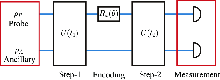
The probe spin ensemble and the ancillary qubit are initially separable, i.e., the input state of the full system is a product state . The whole circuit in Fig. 1 can be described by
| (2) |
where the two steps of evolution last and , respectively. During Step , the probe and ancillary system are entangled. Through the parametric encoding of a negligible evolution time, we obtain a phase parameter by a spin rotation of the probe system. Experimentally can be accumulated during the precessing about -axis Meyer et al. (2001); Gross et al. (2010); Ockeloen et al. (2013) induced by a certain interaction between the probe and a to-be-measured system. Then the rotation about -axis could be performed by a sequence of , where indicates a pulse about -axis. The duration time of Step is determined by under the time-reversal strategy Yurke et al. (1986); Agarwal and Davidovich (2022); Wang et al. (2024). On the last stage of the circuit, a projective measurement about the full system is performed on the output state , whose succuss probability can be used to infer the Fisher information about the estimated parameter. When the input state of the probe (spin ensemble) is an eigenstate of , the maximum parameter information can be obtained only by performing a projective measurement on the ancillary qubit.
It has been shown Yurke et al. (1986); Agarwal and Davidovich (2022); Wang et al. (2024) that the measurement precision can be certainly enhanced such that CFI is increased to be equivalent to QFI when the joint evolution operator becomes the time reversal of , i.e.,
| (3) |
It indicated that the full system traces back its entanglement generation trajectory and returns to the input state if no phase is encoded.
III Conditions for time reversal
According to the definition of in Eq. (2) and the requirement for time reversal in Eq. (3), it is evident that
| (4) | ||||
where is the total spin number of the probe ensemble, is the identity matrix with dimension , is the eigenstate of the operators with eigenvalue , and and denote the ground and excited states of the ancillary spin, respectively. Using the full Hamiltonian (1), we have
| (5) | ||||
where and with . It is found that when
| (6) |
Eq. (4) becomes equivalent to Eq. (5) up to a global phase. Given the expression in Eq. (6), we have
| (7) |
The parity of the probe-spin number determines whether the eigenvalue is an integer or a half-integer. When is even, is an integer and then are the same in parity. A sufficient solution for Eq. (7) is thus . Straightforwardly we have
| (8) |
where ’s, , are proper integers subject to the given magnitudes of , , and . When is odd, are different in parity. The solution can thus be written as
| (9) |
where ’s, , are proper integers. For either even or odd, it might be hard to find the exact solution of if , , and are incommensurable.
The analytical results about can be confirmed by the numerical simulation over the normalized trace of the unitary operator ,
| (10) |
When , we have up to a global phase and vise versa. Once is specified by a unit trace, the time-reversal condition in Eq. (3) is automatically satisfied by setting .
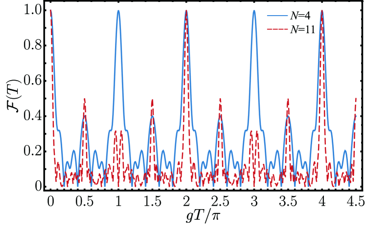
In Fig. 2, we demonstrate the normalized trace as a function of the evolution time exemplified with and under a fixed setting that . The parity of the probe-spin number determines the time when the normalized trace attains unit. When (the even case, see the blue solid line), it is found that the normalized trace attains the maximum value when the full evolution time is a multiple of . For example, when , Eq. (8) is valid for , , and . When (the odd case, see the red dashed line), the normalized trace attains unit when is a multiple of . Particularly, is attained by setting , , and in Eq. (9). Moreover in case of an odd , one can find that the unitary operator becomes
| (11) |
up to a global phase when is an odd multiple of . It will give rise to a vanishing normalized trace . And then the time-reversal strategy is broken. Therefore, choosing a probe ensemble with an even number of spins can significantly accelerate our metrology protocol.
IV Quantum Fisher information
Suppose that we have found an exact solution about on demand of the time-reversal strategy, then the whole unitary evolution operator in Eq. (2) can be rewritten as
| (12) |
Using the Baker-Campbell-Hausdorff formula, we have (the details are provided in Appendix A)
| (13) |
where the phase generator forms as with . We are now on the stage of analyzing the precision limit of the qubit-assisted metrology.
Initially, the ancillary qubit is assumed to be a pure qubit with Kitagawa and Ueda (1993); Jin et al. (2009)
| (14) |
Here and determine the population imbalance and the relative phase between the two bases, respectively. Without loss of generality, we set the azimuthal angle . For the input state of the probe system, always it can be written as
| (15) |
in spectral decomposition, where is the dimension of the density matrix, ’s are the eigenvalues, and ’s are the corresponding eigenstates.
Using Eqs. (14) and (15), QFI of the output state associated with the metrology precision for estimating is given by Braunstein and Caves (1994); Braunstein et al. (1996); Zhang et al. (2013); Liu et al. (2014)
| (16) | ||||
with . We actually obtain a difference between a positive expression, that is vital to achieve Heisenberg scaling as shown in the following, and a non-positive one. A straightforward method to enhance QFI is thus to minimize the magnitude of the second term in Eq. (16) or more generally and precisely to minimize the expression inside the absolute value. Using Eq. (13), we have
| (17) | |||
where . Under a proper state of the ancillary qubit and an optimized evolution time for Step , i.e.,
| (18) |
with an integer , the two terms in Eq. (17) can vanish at the same time for arbitrary probe state . Consequently, Eq. (13) becomes with .
We emphasize that Eq. (17) presents the main advantage of our qubit-assisted metrology over a conventional parameter estimation Giovannetti et al. (2011); Tóth and Apellaniz (2014); Nawrocki (2019); Polino et al. (2020). For a conventional metrology, in which only the probe state is considered, Eq. (17) becomes
| (19) |
Hardly one can find a state-independent time leading to , since and cannot simultaneously become zero.
By Eqs. (16) and (18), QFI becomes the mean square of a phase generator with respect to the probe state, i.e.,
| (20) |
which is a weighted average over the expectation value for the operator within each eigenstate of . Straightforwardly, QFI can attains its peak value when the probe spin ensemble is prepared in a pure state , or , and or a mixed state over them, such as , where with denotes the eigenstate for the optimized collective angular momentum operator . Subjected to the duration time and the time-reversal strategy, the bases ’s are determined by the magnitudes of , , and . Heisenberg scaling can therefore be approached under optimized and .
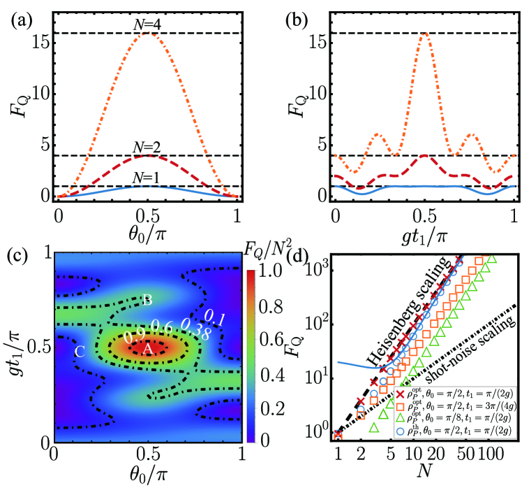
This condition could be confirmed by the numerical simulation in Fig. 3, where the input state of the probe ensemble is set as and the frequencies of both probe spin and ancillary qubit are the same as in Fig. 2. Figure 3(a) describes the dependence of the quantum Fisher information on the input parameter of the ancillary qubit under an optimized evolution time given by Eq. (18). It is shown that follows the Heisenberg scaling when for various . In Fig. 3(b), the initial state of the ancillary qubit is fixed with and finds its peak at as expected by Eq. (18). In both Fig. 3(a) and Fig. 3(b), is symmetrical to the optimized points and varies smoothly around them, indicating that our metrology protocol is not sensitive to the imperfections in parametric control.
In Fig. 3(c), we take and demonstrate the renormalized QFI in the space of and . The black dot-dashed lines are the contour lines indicating the proportional coefficients. The central region around point- describes the most optimized condition that is in agreement with Eq. (18). The surrounding regions about point- and point- describe less optimized conditions with or largely departing from Eq. (18). The behaviors for these points with various are plotted with the red crosses, the orange squares, and the green triangles, respectively, in Fig. 3(d). The first one sticks to its upper bound , and the last two are apparently below this bound. However, a similar behavior to Heisenberg scaling can be restored when is sufficiently large, although or is not optimized.
It is interesting to find that QFI could approach Heisenberg scaling even if the probe ensemble is prepared as a thermal state in the bases of , i.e.,
| (21) |
where is the partition function and is the inverse temperature. By Eqs. (20) and (21), we have
| (22) | ||||
And then for a large probe-spin number, i.e., , it is approximated as
| (23) | ||||
Clearly when . It is indicated that the Heisenberg-scaling behavior dominates QFI at least in the low-temperature limit. And will become divergent in the high-temperature limit, i.e., , which cannot be used to estimate the metrology precision. In Fig. 3(d), the analytical expression in Eq. (23) is confirmed to match the numerical result and both of them approach the Heisenberg scaling, provided .
V Classical Fisher information
In a practical scenario of parametric estimation, CFI is defined by catching the amount of information encoded in the probability distribution for the output state under the estimation process Braun et al. (2018); Liu et al. (2020); Tan et al. (2021). And it is upper bounded by its quantum counterpart on the metrology precision. With the time-reversal strategy, it was shown Yurke et al. (1986); Agarwal and Davidovich (2022); Wang et al. (2024) that CFI can be saturated with QFI, which indicates that all the information encoded in the probe state from the output probability distribution has been extracted. We now derive CFI of our protocol under the same optimized settings in Eq. (18) with as for QFI. For the input state indicated by Eqs. (14) and (15), the output state after the two-step evoluation reads
| (24) | ||||
where ’s are the eigenvalues for the eigenstates of and . Subsequently, we perform the projective measurements on the full system as described in Fig. 1, where with , the eigenstates of for the ancillary qubit. Note ’s are eigenstates of determined by , , and in advance. The probability about detecting the output state in the basis reads
| (25) | ||||
By the probability distribution Braun et al. (2018); Liu et al. (2020); Tan et al. (2021), CFI can be calculated as
| (26) |
The first derivative of with respect to the to-be-estimated phase is and hence
| (27) |
Inserting Eq. (27) to Eq. (26), we have
| (28) | ||||
The last line is exactly the same as Eq. (20) under the optimized condition in Eq. (18), independent of . It is thus verified that QFI can attain its upper-bound in our qubit-assisted metrology. In addition, when the probe is prepared as a polarized state , Eq. (25) reduces to
| (29) |
which implies that the magnitude of can be inferred from the probability and . In this case, only performing the projective measurement on the ancillary qubit yields the Heisenberg-scaling limit .
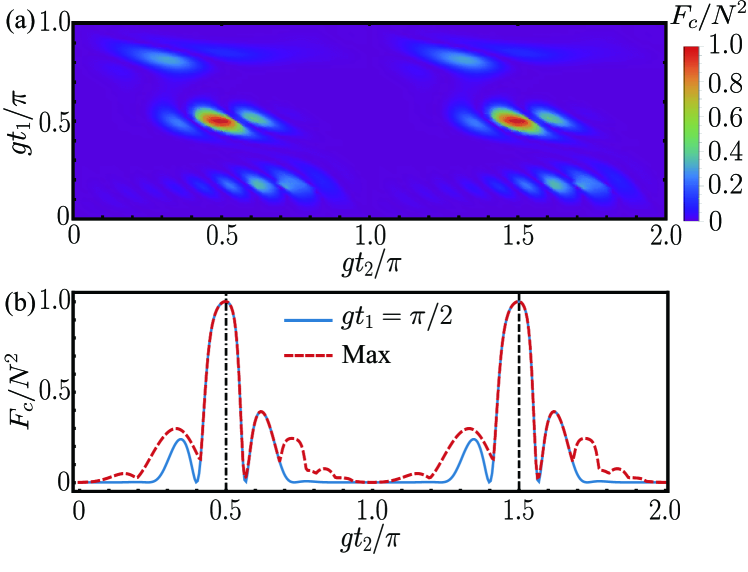
The result about the polarized probe spin ensemble could be confirmed by the numerical simulation of CFI in Fig. 4, where the initial state of the ancillary qubit is optimized with and the frequencies of the two components are the same as in Fig. 3. The dynamics of the output state with a general can be obtained by the unitary operator in Eq. (2) and that under time-reversal strategy is obtained by Eq. (24). And hence can be numerically evaluated by performing the projective measurements on the ancillary qubit. In Fig. 4(a), we plot the renormalized CFI in space of and , when the probe spin number is chosen as an odd number . It is found that the regions around [that is in agreement with Eq. (18) with ] describes the optimized condition for the Heisenberg-scaling metrology. And it can be more clearly described by the blue solid line in Fig. 4(b), when we fix . Moreover, the red dashed line indicates the maximum value of CFI with running from to . One can find that they periodically match with each other. Note the second maximum point in the plot (see the vertical black dashed line) can be predicted by Eq. (9).
It is interesting to find that CFI also attains the Heisenberg scaling when [see the vertical black dot-dashed line in Fig. 4(b)]. It is beyond the sufficient condition for the time-reversal strategy as illustrated by Eq. (9) and Fig. 2. However, it is straightforward to see that when , the full time-evolution operator in the end can be written as , where is given by Eq. (13). Then using Eq. (24), we have and hence the probability distribution in Eq. (29) becomes , which means . It indicates that one can still extract all the information encoded in the probe state from the output probabilities and thus .
VI Discussion
Quantum metrology is conventionally regarded as a parametric-estimation protocol using entanglement or quadratical squeezing to improve the estimation precision beyond the standard quantum limit with respect to the system size . A benchmark result is that the photonic entangled NOON states are capable to attain the Heisenberg scaling characterized with an -dependent quantum Fisher information. However, a feasible implementation is limited to the number of photons or excitations due to the difficulty in generating a large-scale and high-fidelity NOON state Bollinger et al. (1996); Walther et al. (2004); Afek et al. (2010); Zhang et al. (2013), which achieves up to so far in experiment Afek et al. (2010). As for the spin squeezing that is generated in the nonlinear atom-atom interaction platform, the OAT squeezing demonstrates a scaling below the Heisenberg-limited measurement precision with , e.g., in the cold thermal ensembles Hosten et al. (2016), the metrological gain is then found to be up to with atoms.
In contrast, our qubit-assisted metrology protocol can be enhance QFI up to the Heisenberg scaling of with respect to the total probe-spin number , even when the probe system is in a mixed state. More than the interaction between the ancillary qubit and the probe large-spin in the full Hamiltonian (1), our protocol is applicable to another spin-spin-bath model Caldeira et al. (1993); Shao et al. (1996); Xu et al. (2011); Wang and Shao (2012) with Hamiltonian
| (30) |
The corresponding circuit model for the qubit-assisted metrology in Fig. 1 is almost invariant, except that the encoded phase parameter is now obtained by another rotation of the probe system. Thus the circuit is described by
| (31) |
Using the modified full Hamiltonian (30), Eq. (5) becomes
| (32) | ||||
where with . Here and with eigenvalues and denote the eigenstates of the operators and , respectively. According to in Eq. (31) and the time-reversal condition in Eq. (3), we have
| (33) | ||||
Equation (32) becomes equivalent to Eq. (33) up to a global phase when
| (34) |
A sufficient solution for Eq. (34) is found to be independent of the parity of the probe-spin number , and reads,
| (35) |
where ’s, , are proper integers.
With a proper on the time-reversal strategy, the whole unitary evolution operator in Eq. (31) can be rewritten as
| (36) |
Using the Baker-Campbell-Hausdorff formula, we have
| (37) |
where the coefficients of the phase generator are
| (38) | ||||
We are now on the stage of minimizing the magnitude of the second term in Eq. (16) to enhance QFI. With Eqs. (37), (14), and (15), we have
| (39) | ||||
Under a proper state of the ancillary qubit and an optimized evolution time for Step , i.e.,
| (40) |
with an integer , both terms in Eq. (39) can vanish at the same time for arbitrary probe state .
Using Eqs. (16) and (40), QFI becomes the mean square of a phase generator, i.e.,
| (41) |
It reaches the maximum value when the probe spin ensemble is a pure state , or , and or a mixed state over them. Here with denotes the eigenstate for the optimized collective angular momentum operator .
It is evident to see that QFIs in Eqs. (20) and (41) are in the same formation, although with distinct optimized collective angular momentum operator determined by the corresponding interaction Hamiltonian between probe and ancillary qubit. Then following the same optimized procedure from the output state (24) through the first derivative of the probability distribution for the detection (27), one can verify that QFI can attain its upper-bound in our qubit-assisted metrology, i.e., , only by replacing with . Again, when the probe is prepared as a polarized state , the Heisenberg-scaling limit can be attained only by performing the projective measurement on the ancillary qubit.
Since ranges from to , the optimal evolution time in Eq. (40) can only be obtained in the deep strong coupling regime . When , only the second term in Eq. (39) can vanish for arbitrary probe state and the minimum magnitude of the first term associated with can be found at . The optimal condition, that does not render , can thus be rewritten as
| (42) |
with an integer .

In Fig. 5, we show the dependence of QFI on the probe-spin number under various and according to Eq. (40) or Eq. (42) with , where the initial state of the probe ensemble is set as . Numerical simulation confirms that when , QFI attains its peak value . The scaling behavior of QFI gradually deviates from the Heisenberg limit with a decreasing . Yet the numerical fitting for (see the orange solid line and the orange squares) indicate that QFI will follow the Heisenberg scaling in an asymptotic way. It is found that , where the two coefficients are dependent on yet independent of .
VII Conclusion
In summary, we incorporate the joint-evolution-and-quantum-measurement idea to quantum parameter estimation in our metrology protocol. With no input of entangled or squeezed state and with no use of nonlinear Hamiltonian, QFI about the phase encoded into the probe system can be optimized to be the mean square of an optimized phase generator with respect to the probe initial state. That renders an exact or asymptotic Heisenberg-scaling behavior in terms of the spin number even when the probe starts from a thermal state. And the numerical simulation shows that the imperfections in preparing the ancillary qubit and optimizing the evolution time does not change the Heisenberg-scaling behavior about metrology precision as long as is sufficiently large. By virtue of the time-reversal strategy and the projective measurement on the whole system or merely the ancillary qubit, CFI is found to be saturated with its quantum counterpart. Our protocol of qubit-assisted quantum metrology is applicable to a general spin-spin-bath model. It therefore provides an economical way toward the Heisenberg-scaling metrology.
Acknowledgments
We acknowledge financial support from the National Natural Science Foundation of China (Grant No. 11974311).
Appendix A Evolution operator for time-reversal strategy in the qubit-assisted metrology
This appendix derives the unitary evolution operator for the time-reversal strategy in our qubit-assisted metrology. With the time-reversal condition (3), the whole evolution operator in Eq. (12) can be written as
| (43) | ||||
Using the full Hamiltonian (1) and the commutation relation ,
| (44) | ||||
In the last step, we have used . The Baker-Campbell-Hausdorff formula yields:
| (45) |
where and . Using the commutation relation with the Levi-Civita tensor, we have
| (46) | ||||
and so on. Equation (45) thus becomes
| (47) | ||||
And similarly, we have
| (48) |
Therefore, Eq. (44) can be reduced to
| (49) | ||||
and hence
| (50) |
where and . It is exactly Eq. (13) in the main text.
References
- Sun et al. (2010) Z. Sun, J. Ma, X.-M. Lu, and X. Wang, Fisher information in a quantum-critical environment, Phys. Rev. A 82, 022306 (2010).
- Ma et al. (2011) J. Ma, Y.-x. Huang, X. Wang, and C. P. Sun, Quantum fisher information of the greenberger-horne-zeilinger state in decoherence channels, Phys. Rev. A 84, 022302 (2011).
- Genoni et al. (2012) M. G. Genoni, S. Olivares, D. Brivio, S. Cialdi, D. Cipriani, A. Santamato, S. Vezzoli, and M. G. A. Paris, Optical interferometry in the presence of large phase diffusion, Phys. Rev. A 85, 043817 (2012).
- Escher et al. (2012) B. M. Escher, L. Davidovich, N. Zagury, and R. L. de Matos Filho, Quantum metrological limits via a variational approach, Phys. Rev. Lett. 109, 190404 (2012).
- Zhong et al. (2013) W. Zhong, Z. Sun, J. Ma, X. Wang, and F. Nori, Fisher information under decoherence in bloch representation, Phys. Rev. A 87, 022337 (2013).
- Paris (2009) M. G. Paris, Quantum estimation for quantum technology, Int. J. Quantum Inf. 7, 125 (2009).
- Helstrom (1969) C. W. Helstrom, Quantum detection and estimation theory, J. Stat. Phys. 1, 231 (1969).
- Yurke et al. (1986) B. Yurke, S. L. McCall, and J. R. Klauder, Su(2) and su(1,1) interferometers, Phys. Rev. A 33, 4033 (1986).
- Caves (1981) C. M. Caves, Quantum-mechanical noise in an interferometer, Phys. Rev. D 23, 1693 (1981).
- Taylor and Bowen (2016) M. A. Taylor and W. P. Bowen, Quantum metrology and its application in biology, Phys. Rep. 615, 1 (2016).
- Mauranyapin et al. (2017) N. Mauranyapin, L. Madsen, M. Taylor, M. Waleed, and W. Bowen, Evanescent single-molecule biosensing with quantum-limited precision, Nat. Photonics 11, 477 (2017).
- Ludlow et al. (2015) A. D. Ludlow, M. M. Boyd, J. Ye, E. Peik, and P. O. Schmidt, Optical atomic clocks, Rev. Mod. Phys. 87, 637 (2015).
- Katori (2011) H. Katori, Optical lattice clocks and quantum metrology, Nat. Photonics 5, 203 (2011).
- Jones et al. (2009) J. A. Jones, S. D. Karlen, J. Fitzsimons, A. Ardavan, S. C. Benjamin, G. A. D. Briggs, and J. J. Morton, Magnetic field sensing beyond the standard quantum limit using 10-spin noon states, Science 324, 1166 (2009).
- Giovannetti et al. (2011) V. Giovannetti, S. Lloyd, and L. Maccone, Advances in quantum metrology, Nat. Photonics 5, 222 (2011).
- Tóth and Apellaniz (2014) G. Tóth and I. Apellaniz, Quantum metrology from a quantum information science perspective, J. Phys. A: Math. Theor. 47, 424006 (2014).
- Nawrocki (2019) W. Nawrocki, Introduction to quantum metrology, 2nd ed. (Springer Nature Switzerland, Cham, Switzerland, 2019).
- Polino et al. (2020) E. Polino, M. Valeri, N. Spagnolo, and F. Sciarrino, Photonic quantum metrology, AVS Quantum Sci. 2, 024703 (2020).
- Holevo (1982) A. S. Holevo, Probabilistic and statistical aspects of quantum theory (North-Holland, Amsterdam, 1982).
- Braunstein and Caves (1994) S. L. Braunstein and C. M. Caves, Statistical distance and the geometry of quantum states, Phys. Rev. Lett. 72, 3439 (1994).
- Braunstein et al. (1996) S. L. Braunstein, C. M. Caves, and G. J. Milburn, Generalized uncertainty relations: theory, examples, and lorentz invariance, Ann. Phys. 247, 135 (1996).
- Luo (2003) S. Luo, Wigner-yanase skew information and uncertainty relations, Phys. Rev. Lett. 91, 180403 (2003).
- Pezzé and Smerzi (2009) L. Pezzé and A. Smerzi, Entanglement, nonlinear dynamics, and the heisenberg limit, Phys. Rev. Lett. 102, 100401 (2009).
- Kacprowicz et al. (2010) M. Kacprowicz, R. Demkowicz-Dobrzański, W. Wasilewski, K. Banaszek, and I. Walmsley, Experimental quantum-enhanced estimation of a lossy phase shift, Nat. Photonics 4, 357 (2010).
- Leibfried et al. (2004) D. Leibfried, M. D. Barrett, T. Schaetz, J. Britton, J. Chiaverini, W. M. Itano, J. D. Jost, C. Langer, and D. J. Wineland, Toward heisenberg-limited spectroscopy with multiparticle entangled states, Science 304, 1476 (2004).
- Mitchell et al. (2004) M. W. Mitchell, J. S. Lundeen, and A. M. Steinberg, Super-resolving phase measurements with a multiphoton entangled state, Nature 429, 161 (2004).
- Boto et al. (2000) A. N. Boto, P. Kok, D. S. Abrams, S. L. Braunstein, C. P. Williams, and J. P. Dowling, Quantum interferometric optical lithography: Exploiting entanglement to beat the diffraction limit, Phys. Rev. Lett. 85, 2733 (2000).
- Gerry (2000) C. C. Gerry, Heisenberg-limit interferometry with four-wave mixers operating in a nonlinear regime, Phys. Rev. A 61, 043811 (2000).
- Bollinger et al. (1996) J. J. Bollinger, W. M. Itano, D. J. Wineland, and D. J. Heinzen, Optimal frequency measurements with maximally correlated states, Phys. Rev. A 54, R4649 (1996).
- Walther et al. (2004) P. Walther, J.-W. Pan, M. Aspelmeyer, R. Ursin, S. Gasparoni, and A. Zeilinger, De broglie wavelength of a non-local four-photon state, Nature 429, 158 (2004).
- Afek et al. (2010) I. Afek, O. Ambar, and Y. Silberberg, High-noon states by mixing quantum and classical light, Science 328, 879 (2010).
- Zhang et al. (2013) Y. M. Zhang, X. W. Li, W. Yang, and G. R. Jin, Quantum fisher information of entangled coherent states in the presence of photon loss, Phys. Rev. A 88, 043832 (2013).
- Wineland et al. (1992) D. J. Wineland, J. J. Bollinger, W. M. Itano, F. L. Moore, and D. J. Heinzen, Spin squeezing and reduced quantum noise in spectroscopy, Phys. Rev. A 46, R6797 (1992).
- Kitagawa and Ueda (1993) M. Kitagawa and M. Ueda, Squeezed spin states, Phys. Rev. A 47, 5138 (1993).
- Wineland et al. (1994) D. J. Wineland, J. J. Bollinger, W. M. Itano, and D. J. Heinzen, Squeezed atomic states and projection noise in spectroscopy, Phys. Rev. A 50, 67 (1994).
- Goda et al. (2008) K. Goda, O. Miyakawa, E. E. Mikhailov, S. Saraf, R. Adhikari, K. McKenzie, R. Ward, S. Vass, A. J. Weinstein, and N. Mavalvala, A quantum-enhanced prototype gravitational-wave detector, Nat. Phys. 4, 472 (2008).
- Liu et al. (2011) Y. C. Liu, Z. F. Xu, G. R. Jin, and L. You, Spin squeezing: Transforming one-axis twisting into two-axis twisting, Phys. Rev. Lett. 107, 013601 (2011).
- Zhang et al. (2017) Y.-C. Zhang, X.-F. Zhou, X. Zhou, G.-C. Guo, and Z.-W. Zhou, Cavity-assisted single-mode and two-mode spin-squeezed states via phase-locked atom-photon coupling, Phys. Rev. Lett. 118, 083604 (2017).
- Gross et al. (2010) C. Gross, T. Zibold, E. Nicklas, J. Esteve, and M. K. Oberthaler, Nonlinear atom interferometer surpasses classical precision limit, Nature 464, 1165 (2010).
- Riedel et al. (2010) M. F. Riedel, P. Böhi, Y. Li, T. W. Hänsch, A. Sinatra, and P. Treutlein, Atom-chip-based generation of entanglement for quantum metrology, Nature 464, 1170 (2010).
- Bohnet et al. (2016) J. G. Bohnet, B. C. Sawyer, J. W. Britton, M. L. Wall, A. M. Rey, M. Foss-Feig, and J. J. Bollinger, Quantum spin dynamics and entanglement generation with hundreds of trapped ions, Science 352, 1297 (2016).
- Lu et al. (2019) Y. Lu, S. Zhang, K. Zhang, W. Chen, Y. Shen, J. Zhang, J.-N. Zhang, and K. Kim, Global entangling gates on arbitrary ion qubits, Nature 572, 363 (2019).
- Song et al. (2019) C. Song, K. Xu, H. Li, Y.-R. Zhang, X. Zhang, W. Liu, Q. Guo, Z. Wang, W. Ren, J. Hao, et al., Generation of multicomponent atomic schrödinger cat states of up to 20 qubits, Science 365, 574 (2019).
- Xu et al. (2020) K. Xu, Z.-H. Sun, W. Liu, Y.-R. Zhang, H. Li, H. Dong, W. Ren, P. Zhang, F. Nori, D. Zheng, et al., Probing dynamical phase transitions with a superconducting quantum simulator, Sci. Adv. 6, eaba4935 (2020).
- Hosten et al. (2016) O. Hosten, N. J. Engelsen, R. Krishnakumar, and M. A. Kasevich, Measurement noise 100 times lower than the quantum-projection limit using entangled atoms, Nature 529, 505 (2016).
- Bao et al. (2020) H. Bao, J. Duan, S. Jin, X. Lu, P. Li, W. Qu, M. Wang, I. Novikova, E. E. Mikhailov, K.-F. Zhao, et al., Spin squeezing of 1011 atoms by prediction and retrodiction measurements, Nature 581, 159 (2020).
- Duan et al. (2024) J. Duan, Z. Hu, X. Lu, L. Xiao, S. Jia, K. Mølmer, and Y. Xiao, Continuous field tracking with machine learning and steady state spin squeezing, arXiv:2402.00536 (2024).
- Borregaard et al. (2017) J. Borregaard, E. Davis, G. S. Bentsen, M. H. Schleier-Smith, and A. S. Sørensen, One-and two-axis squeezing of atomic ensembles in optical cavities, New J. Phys. 19, 093021 (2017).
- Helmerson and You (2001) K. Helmerson and L. You, Creating massive entanglement of bose-einstein condensed atoms, Phys. Rev. Lett. 87, 170402 (2001).
- Macrì et al. (2020) V. Macrì, F. Nori, S. Savasta, and D. Zueco, Spin squeezing by one-photon–two-atom excitation processes in atomic ensembles, Phys. Rev. A 101, 053818 (2020).
- Li et al. (2014) D. Li, C.-H. Yuan, Z. Ou, and W. Zhang, The phase sensitivity of an su (1, 1) interferometer with coherent and squeezed-vacuum light, New J. Phys. 16, 073020 (2014).
- Li et al. (2016) D. Li, B. T. Gard, Y. Gao, C.-H. Yuan, W. Zhang, H. Lee, and J. P. Dowling, Phase sensitivity at the heisenberg limit in an su(1,1) interferometer via parity detection, Phys. Rev. A 94, 063840 (2016).
- Jing et al. (2011) J. Jing, C. Liu, Z. Zhou, Z. Ou, and W. Zhang, Realization of a nonlinear interferometer with parametric amplifiers, Appl. Phys. Lett. 99, 011110 (2011).
- Hudelist et al. (2014) F. Hudelist, J. Kong, C. Liu, J. Jing, Z. Ou, and W. Zhang, Quantum metrology with parametric amplifier-based photon correlation interferometers, Nat. Commun. 5, 3049 (2014).
- Du et al. (2022) W. Du, J. Kong, G. Bao, P. Yang, J. Jia, S. Ming, C.-H. Yuan, J. F. Chen, Z. Y. Ou, M. W. Mitchell, and W. Zhang, Su(2)-in-su(1,1) nested interferometer for high sensitivity, loss-tolerant quantum metrology, Phys. Rev. Lett. 128, 033601 (2022).
- Marino et al. (2012) A. M. Marino, N. V. Corzo Trejo, and P. D. Lett, Effect of losses on the performance of an su(1,1) interferometer, Phys. Rev. A 86, 023844 (2012).
- Xia et al. (2024) B. Xia, J. Huang, H. Li, Z. Luo, and G. Zeng, Nanoradian-scale precision in light rotation measurement via indefinite quantum dynamics, arXiv:2310.07125 (2024).
- Agarwal and Davidovich (2022) G. S. Agarwal and L. Davidovich, Quantifying quantum-amplified metrology via fisher information, Phys. Rev. Res. 4, L012014 (2022).
- Wang et al. (2024) J. Wang, R. L. d. M. Filho, G. S. Agarwal, and L. Davidovich, Quantum advantage of time-reversed ancilla-based metrology of absorption parameters, Phys. Rev. Res. 6, 013034 (2024).
- Luo and Yu (2023) D.-W. Luo and T. Yu, Time-reversal assisted quantum metrology with an optimal control, arXiv:2312.14443 (2023).
- Gillard et al. (2022) G. Gillard, E. Clarke, and E. A. Chekhovich, Harnessing many-body spin environment for long coherence storage and high-fidelity single-shot qubit readout, Nat. Commun. 13, 4048 (2022).
- Pyrkov and Byrnes (2013) A. N. Pyrkov and T. Byrnes, Entanglement generation in quantum networks of bose–einstein condensates, New J. Phys. 15, 093019 (2013).
- Meyer et al. (2001) V. Meyer, M. A. Rowe, D. Kielpinski, C. A. Sackett, W. M. Itano, C. Monroe, and D. J. Wineland, Experimental demonstration of entanglement-enhanced rotation angle estimation using trapped ions, Phys. Rev. Lett. 86, 5870 (2001).
- Ockeloen et al. (2013) C. F. Ockeloen, R. Schmied, M. F. Riedel, and P. Treutlein, Quantum metrology with a scanning probe atom interferometer, Phys. Rev. Lett. 111, 143001 (2013).
- Jin et al. (2009) G.-R. Jin, Y.-C. Liu, and W.-M. Liu, Spin squeezing in a generalized one-axis twisting model, New J. Phys. 11, 073049 (2009).
- Liu et al. (2014) J. Liu, X.-X. Jing, W. Zhong, and X.-G. Wang, Quantum fisher information for density matrices with arbitrary ranks, Commun. Theor. Phys. 61, 45 (2014).
- Braun et al. (2018) D. Braun, G. Adesso, F. Benatti, R. Floreanini, U. Marzolino, M. W. Mitchell, and S. Pirandola, Quantum-enhanced measurements without entanglement, Rev. Mod. Phys. 90, 035006 (2018).
- Liu et al. (2020) J. Liu, H. Yuan, X.-M. Lu, and X. Wang, Quantum fisher information matrix and multiparameter estimation, J. Phys. A: Math. Theor. 53, 023001 (2020).
- Tan et al. (2021) K. C. Tan, V. Narasimhachar, and B. Regula, Fisher information universally identifies quantum resources, Phys. Rev. Lett. 127, 200402 (2021).
- Caldeira et al. (1993) A. O. Caldeira, A. H. Castro Neto, and T. Oliveira de Carvalho, Dissipative quantum systems modeled by a two-level-reservoir coupling, Phys. Rev. B 48, 13974 (1993).
- Shao et al. (1996) J. Shao, M.-L. Ge, and H. Cheng, Decoherence of quantum-nondemolition systems, Phys. Rev. E 53, 1243 (1996).
- Xu et al. (2011) J. Xu, J. Jing, and T. Yu, Entanglement dephasing dynamics driven by a bath of spins, J. Phys. A: Math. Theor. 44, 185304 (2011).
- Wang and Shao (2012) H. Wang and J. Shao, Dynamics of a two-level system coupled to a bath of spins, J. Chem. Phys. 137, 22A504 (2012).