Learning to Cut via Hierarchical Sequence/Set Model for Efficient Mixed-Integer Programming

Abstract

Cutting planes (cuts) play an important role in solving mixed-integer linear programs (MILPs), which formulate many important real-world applications. Cut selection heavily depends on (P1) which cuts to prefer and (P2) how many cuts to select. Although modern MILP solvers tackle (P1)-(P2) by human-designed heuristics, machine learning carries the potential to learn more effective heuristics. However, many existing learning-based methods learn which cuts to prefer, neglecting the importance of learning how many cuts to select. Moreover, we observe that (P3) what order of selected cuts to prefer significantly impacts the efficiency of MILP solvers as well. To address these challenges, we propose a novel hierarchical sequence/set model (HEM) to learn cut selection policies. Specifically, HEM is a bi-level model: (1) a higher-level module that learns how many cuts to select, (2) and a lower-level module—that formulates the cut selection as a sequence/set to sequence learning problem—to learn policies selecting an ordered subset with the cardinality determined by the higher-level module. To the best of our knowledge, HEM is the first data-driven methodology that well tackles (P1)-(P3) simultaneously. Experiments demonstrate that HEM significantly improves the efficiency of solving MILPs on eleven challenging MILP benchmarks, including two Huawei’s real problems.

1 Introduction

Mixed-integer linear programming (MILP)—which aims to optimize a linear objective subject to linear constraints and integer constraints (i.e., some or all of the variables are integer-valued)—is one of the most fundamental mathematical models [1, 2]. MILP is applicable to a wide range of important real-world applications, such as supply chain management [3], production planning [4], scheduling [5], vehicle routing [6], facility location [7], bin packing [8], etc. A standard MILP takes the form of

$$z^{*}\triangleq\min_{\textbf{x}}\{\textbf{c}^{\top}\textbf{x}|\textbf{A}\textbf{x}\leq\textbf{b},\textbf{x}\in\mathbb{R}^{n},x_{j}\in\mathbb{Z}\,\,\text{for all }j\in\mathcal{I}\}.$$ (1)

Here $\textbf{c}\in\mathbb{R}^{n}$, $\textbf{A}\in\mathbb{R}^{m\times n}$, $\textbf{b}\in\mathbb{R}^{m}$, $x_{j}$ denotes the $j$-th entry of vector x, $\mathcal{I}\subseteq\{1,\dots,n\}$ denotes the set of indices of integer variables, and $z^{*}$ denotes the optimal objective value of Problem (1). However, it can be extremely hard to solve MILPs, as MILPs are $\mathcal{NP}$-hard problems [1].

Many modern MILP solvers [9, 10, 11] solve MILPs by a branch-and-bound tree search algorithm [12]. It builds a tree where it solves a linear programming (LP) relaxation of a MILP (Problem (1) or its subproblems) at each node. To improve the efficiency of the tree search algorithm, cutting planes (cuts) [13] are introduced in the attempt to strengthen the LP relaxations [2, 14]. Existing work on cuts falls into two categories: cut generation and cut selection [15]. Cut generation aims to generate candidate cuts, i.e., valid linear inequalities that strengthen the LP relaxations [2]. Researchers have theoretically studied many families of both general-purpose and class specific cuts [16]. Nevertheless, it poses a computational challenge if adding all generated cuts to the LP relaxations [17, 18]. To address this challenge, cut selection is a common idea to further improve the efficiency of solving MILPs by selecting a proper subset of the generated cuts [17, 18, 15]. In this paper, we focus on the cut selection problem, which plays an important role in terms of the efficiency of MILP solvers [2, 19, 16].

Cut selection heavily depends on (P1) which cuts to prefer and (P2) how many cuts to select [2, 18]. To tackle (P1)-(P2), many modern MILP solvers [9, 10, 11] employ manually-designed heuristics. However, it is difficult for hard-coded heuristics to take into account underlying patterns among MILPs collected from certain types of real-world applications, e.g., day-to-day production planning, bin packing, and vehicle routing problems [20, 6, 8]. To enhance modern MILP solvers, recent methods [19, 16, 15, 21] propose to learn cut selection policies via machine learning, especially reinforcement learning. Specifically, many existing learning-based methods [19, 16, 21] learn a scoring function to measure cut quality and select a fixed ratio/number of cuts with high scores. They carry the potential to learn more effective heuristics, as they can effectively capture underlying patterns among MILPs collected from specific applications [14, 19, 16, 15].

However, the aforementioned learning-based methods suffer from two limitations. First, they learn which cuts to prefer by learning a scoring function, without learning how many cuts to select [18, 17]. Moreover, we observe from extensive empirical results that (P3) what order of selected cuts to prefer has a significant impact on the efficiency of solving MILPs as well (see Section 4.1). Second, they do not take into account the interaction among cuts when learning which cuts to prefer, as they score each cut independently. Consequently, they struggle to select cuts complementary to each other, which could severely degrade the efficiency of solving MILPs [18]. Indeed, we empirically show that they tend to select many similar cuts with high scores, while many selected cuts are possibly redundant and increase the computational burden (see Section 8.6.1).

To tackle the aforementioned problems, we propose a novel hierarchical sequence/set model (HEM) to learn cut selection policies via reinforcement learning (RL). To the best of our knowledge, HEM is the first data-driven methodology that can well tackle (P1)-(P3) in cut selection simultaneously. Specifically, HEM is a bi-level model: (1) a higher-level module to learn the number of cuts that should be selected, (2) and a lower-level module to learn policies selecting an ordered subset with the cardinality determined by the higher-level module. The lower-level module formulates the cut selection task as a novel sequence/set to sequence (Seq2Seq/Set2Seq) learning problem, which leads to two major advantages. First, the Seq2Seq/Set2Seq model is popular in capturing the underlying order information [22], which is critical for tackling (P3). Second, the Seq2Seq/Set2Seq model can well capture the interaction among cuts, as it models the joint conditional probability of the selected cuts given an input sequence/set of the candidate cuts. As a result, experiments demonstrate that HEM significantly and consistently outperforms competitive baselines in terms of solving efficiency on three synthetic and eight challenging MILP benchmarks. The MILP problems include some benchmarks from MIPLIB 2017 [23], and large-scale real-world problems at Google and Huawei. Therefore, the powerful performance of HEM demonstrates its promising potential for enhancing modern MILP solvers in real-world applications. Moreover, experiments demonstrate that HEM well generalizes to MILPs that are significantly larger than those in the training data.

We summarize our major contributions as follows. (1) We observe an important problem in cut selection, i.e., what order of selected cuts to prefer has a significant impact on the efficiency of solving MILPs (see Section 4.1). (2) To the best of our knowledge, our proposed HEM is the first data-driven methodology that is able to tackle (P1)-(P3) in cut selection simultaneously. (3) We formulate the cut selection task as a novel sequence/set to sequence learning problem, which captures not only the underlying order information, but also the interaction among cuts to select cuts complementary to each other. (4) Experiments demonstrate that HEM achieves significant and consistent improvements over competitive baselines on challenging MILP problems, including some benchmarks from MIPLIB 2017 and large-scale real-world problems at Google and Huawei.

An earlier version of this paper has been published at ICLR 2023 [24]. This journal manuscript significantly extends the conference version by proposing an enhanced version of HEM, namely HEM++, which further improves HEM in terms of the formulation, policy, and training method, respectively. (1) Regarding the formulation, HEM++ extends the formulation to the multiple rounds setting—which is widely applicable in real-world scenarios—while HEM mainly focuses on training policies under the one round setting (see Section 6.1). (2) Regarding the policy, HEM++ formulates the model as a set to sequence model instead of a sequence to sequence (i.e., the model in HEM), which improves the representation of input cuts by removing redundant input-order information (see Section 6.2). (3) Regarding the training method, HEM++ proposes a hierarchical proximal policy optimization method, which further improves sample efficiency (see Section 6.3). Sample-efficient training is important for learning cut selection, especially under the multiple rounds setting, as the action space is large and increases exponentially with the number of cut separation rounds. Experiments demonstrate the superiority of HEM++ in Section 8.3. In addition to HEM++, this paper further deploys HEM to Huawei’s real production scenario to evaluate its effectiveness (see Sections 7 and 8.7), and conducts visualization experiments to provide further insight into our method (see Section 8.6).

2 Related work

The use of machine learning to improve the MILP solver performance has been an active topic of significant interest in recent years [14, 25, 26, 27, 19]. During the solving process of the solvers, many crucial decisions that significantly impact the solver performance are based on heuristics [2]. Recent methods propose to learn more effective heuristics via machine learning from MILPs collected from specific applications [14, 28]. This line of research has shown significant improvement on the solver performance, including cut selection [19, 16, 15, 29], variable selection [30, 27, 31, 32], node selection [33, 34], column generation [35], and primal heuristics selection [36, 37].

In this paper, we focus on cut selection, which plays an important role in modern MILP solvers [18, 17]. For cut selection, many existing learning-based methods [19, 16, 21] focus on learning which cuts should be preferred by learning a scoring function to measure cut quality. Specifically, [19] proposes a reinforcement learning approach to learn to select the best Gomory cut [13]. Furthermore, [16] proposes to learn to select a cut that yield the best dual bound improvement via imitation learning. Instead of selecting the best cut, [21] frames cut selection as multiple instance learning to learn a scoring function, and selects a fixed ratio of cuts with high scores. However, they suffer from two limitations as mentioned in Section 1. In addition, [15] proposes to learn weightings of four expert-designed scoring rules. On the theoretical side, [38, 39] has provided some provable guarantees for learning cut selection policies.

3 Background

3.1 Cutting planes

Given the MILP problem in (1), we drop all its integer constraints to obtain its linear programming (LP) relaxation, which takes the form of

$$z_{\text{LP}}^{*}\triangleq\min_{\textbf{x}}\{\textbf{c}^{\top}\textbf{x}|\textbf{A}\textbf{x}\leq\textbf{b},\textbf{x}\in\mathbb{R}^{n}\}.$$ (2)

As the problem in (2) expands the feasible set of the problem in (1), we have $z_{\text{LP}}^{*}\leq z^{*}$. We denote any lower bound found via an LP relaxation by a dual bound. Given the LP relaxation in (2), cutting planes (cuts) are linear inequalities that are added to the LP relaxation to tighten it without removing any integer feasible solutions of (1). Cuts generated by MILP solvers are added in successive rounds. Specifically, each round $k$ involves (i) solving the current LP relaxation, (ii) generating a pool of candidate cuts $\mathcal{C}^{k}$, (iii) selecting a subset $\mathcal{S}^{k}\subseteq\mathcal{C}^{k}$, (iv) adding $\mathcal{S}^{k}$ to the current LP relaxation to obtain the next LP relaxation, (v) and proceeding to the next round. Adding all the generated cuts to the LP relaxation would maximally strengthen the LP relaxation and improve the lower bound at each round. However, adding too many cuts could lead to large models, which can increase the computational burden and present numerical instabilities [17, 16]. Therefore, cut selection is proposed to select a proper subset of the candidate cuts, which is significant for improving the efficiency of solving MILPs [18, 19].

3.2 Branch-and-cut

In modern MILP solvers, cutting planes are often combined with the branch-and-bound algorithm [12], which is known as the branch-and-cut algorithm [40]. Branch-and-bound techniques perform implicit enumeration by building a search tree, in which every node represents a subproblem of the original problem in (1). The solving process begins by selecting a leaf node of the tree and solving its LP relaxation. Let $\textbf{x}^{*}$ be the optimal solution of the LP relaxation. If $\textbf{x}^{*}$ violates the original integrality constraints, two subproblems (child nodes) of the leaf node are created by branching. Specifically, the leaf node is added with constraints $x_{i}\leq\lfloor x_{i}^{*}\rfloor\,\,\text{and}\,\,x_{i}\geq\lceil x_{i}^{*}\rceil$, respectively, where $x_{i}$ denotes the $i$-th variable, $x_{i}^{*}$ denotes the $i$-th entry of vector $\textbf{x}^{*}$, and $\lfloor\rfloor$ and $\lceil\rceil$ denote the floor and ceil functions. In contrast, if $\textbf{x}^{*}$ is a (mixed-)integer solution of (1), then we obtain an upper bound on the optimal objective value of (1), which we denote by primal bound. In modern MILP solvers, the addition of cutting planes is alternated with the branching phase. That is, cuts are added at search tree nodes before branching to tighten their LP relaxations. As strengthening the relaxation before starting to branch is decisive to ensure an efficient tree search [17, 14], we focus on adding cuts at the root node, which follows [27, 16].

3.3 Primal-dual gap integral

We keep track of two important bounds when running branch-and-cut, i.e., the global primal and dual bounds, which are the best upper and lower bounds on the optimal objective value of Problem (1), respectively. We define the primal-dual gap integral (PD integral) by the area between the curve of the solver’s global primal bound and the curve of the solver’s global dual bound. The PD integral is a widely used metric for evaluating solver performance [26, 41]. For example, the primal-dual gal integral is used as a primary evaluation metric in the NeurIPS 2021 ML4CO competition [26]. Moreover, We define the primal-dual gap by the difference between the global primal and dual bounds.

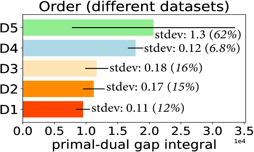
(a) Evaluate RandomAll on five different datasets.

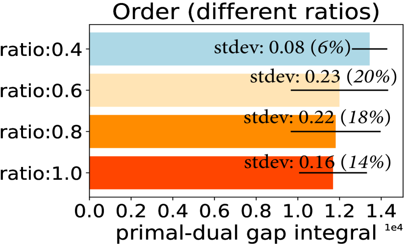
(b) Evaluate RandomNv on MIPLIB mixed neos.

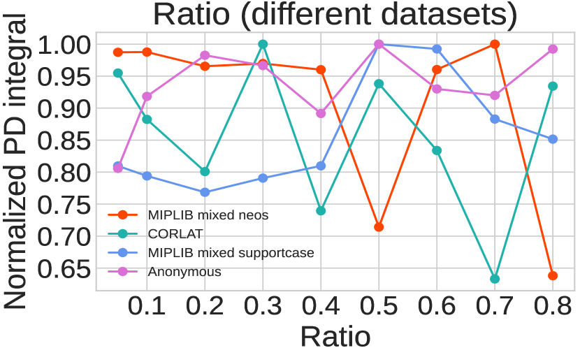
(c) Evaluate NV with different ratios on four datasets.

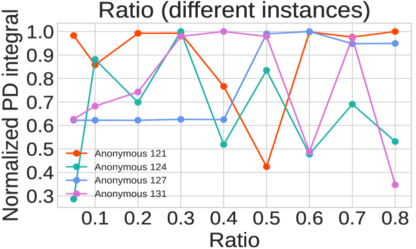
(d) Evaluate NV with different ratios on Anonymous.

Figure 1: (a)-(b) We design two cut selection heuristics, namely RandomAll and RandomNV (see Section 4.1 for details), which both add the same subset of cuts in random order for a given MILP. The results in (a) and (b) show that adding the same selected cuts in different order leads to variable overall solver performance. (c)-(d) We use the Normalized Violation (NV) heuristics [21] in the following experiments. The results in (c) show that the performance of NV varies widely with the given ratios across different datasets. The results in (d) show that the performance of NV varies widely with the given ratios across different instances from the Anonymous dataset.

4 Motivating results

In this section, we first empirically show that the order of selected cuts, i.e., the selected cuts are added to the LP relaxations in this order, significantly impacts the efficiency of solving MILPs. Moreover, we then empirically show that the ratio of selected cuts significantly impacts the efficiency of solving MILPs as well. Please see Appendix B.1 for details of the datasets used in this section.

4.1 Order matters

Previous work [42, 43, 44, 45] has shown that the order of constraints for a given linear program (LP) significantly impacts its constructed initial basis, which is important for solving the LP. As a cut is a linear constraint, adding cuts to the LP relaxations is equivalent to adding constraints to the LP relaxations. Therefore, the order of added cuts could have a significant impact on solving the LP relaxations as well, thus being important for solving MILPs. Indeed, our empirical results show that this is the case. (1) We design a RandomAll cut selection rule, which randomly permutes all the candidate cuts, and adds all the cuts to the LP relaxations in the random order. We evaluate RandomAll on five challenging datasets, namely D1, D2, D3, D4, and D5. We use the SCIP 8.0.0 [10] as the backend solver, and evaluate the solver performance by the average PD integral within a time limit of 300 seconds. We evaluate RandomAll on each dataset over ten random seeds, and each bar in Figure 1(a) shows the mean and standard deviation (stdev) of its performance on each dataset. As shown in Figure 1(a), the performance of RandomAll on each dataset varies widely with the order of selected cuts. (2) We further design a RandomNV cut selection rule. RandomNV is different from RandomAll in that it selects a given ratio of the candidate cuts rather than all the cuts. RandomNV first scores each cut using the Normalized Violation [21] and selects a given ratio of cuts with high scores. It then randomly permutes the selected cuts. Each bar in Figure 1(b) shows the mean and stdev of the performance of RandomNV with a given ratio on the same dataset. Figures 1(a) and 1(b) show that adding the same selected cuts in different order leads to variable solver performance, which demonstrates that the order of selected cuts is important for solving MILPs.

4.2 Ratio matters

We use the Normalized Violation (NV) [21] method in the following experiments. (1) We first evaluate the NV methods that select different ratios of candidate cuts on four datasets. Each line in Fig. 1(c) shows the performance (normalized average PD integral) of NV with different given ratios of selected cuts on each dataset. The results in Fig. 1(c) show that the performance of NV varies widely with the ratio of selected cuts. Moreover, the results demonstrate that the ratio that leads to better solver performance is variable across different datasets, suggesting that learning dataset-dependent ratios is important. (2) We then evaluate the NV methods that select different ratios of candidate cuts on four instances from the Anonymous dataset. Each line in Fig. 1(d) shows the performance (normalized average PD integral) of NV with different given ratios of selected cuts on each instance. The results in Fig. 1(d) show that the performance of NV varies widely with the ratio of selected cuts. Moreover, the results demonstrate that the ratio that leads to better solver performance is variable across different instances, which suggests that learning instance-dependent ratios is important for cut selection as well.

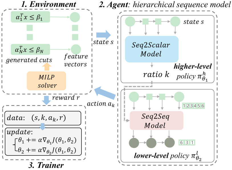
Figure 2: Illustration of our proposed RL framework for learning cut selection policies. We formulate a MILP solver as the environment and the HEM as the agent. Moreover, we train HEM via hierarchical policy gradients.

5 Learning Cut Selection via Hierarchical Sequence Model (HEM)

For cut selection, the optimal subsets that should be selected are inaccessible, while one can assess the quality of selected subsets using a solver and provide the feedbacks to learning algorithms. Therefore, we leverage reinforcement learning (RL) to learn cut selection policies. In this section, we provide a detailed description of our proposed RL framework for learning cut selection as shown in Fig 2. First, we present our formulation of the cut selection as a Markov decision process (MDP) [46] in Section 5.1. Second, we present a detailed description of our proposed HEM in Section 5.2. Finally, we derive a hierarchical policy gradient for training HEM under the one round setting in Section 5.3.

5.1 Reinforcement Learning Formulation

As shown in Fig 2, we formulate a MILP solver as the environment and our proposed HEM as the agent. We consider an MDP defined by the tuple $(\mathcal{S},\mathcal{A},r,f)$. Specifically, we specify the state space $\mathcal{S}$, the action space $\mathcal{A}$, the reward function $r:\mathcal{S}\times\mathcal{A}\to\mathbb{R}$, the transition function $f$, and the terminal state in the following. (1) The state space $\mathcal{S}$. Since the current LP relaxation and the generated cuts contain the core information for cut selection, we define a state $s$ by $(M_{\text{LP}},\mathcal{C},\textbf{x}_{\text{LP}}^{*})$. Here $M_{\text{LP}}$ denotes the mathematical model of the current LP relaxation, $\mathcal{C}$ denotes the set of the candidate cuts, and $\textbf{x}_{\text{LP}}^{*}$ denotes the optimal solution of the LP relaxation. To encode the state information, we follow [2, 21] to design thirteen features for each candidate cut based on the information of $(M_{\text{LP}},\mathcal{C},\textbf{x}_{\text{LP}}^{*})$. That is, we actually represent a state $s$ by a sequence of thirteen-dimensional feature vectors. We present details of the designed features in Appendix LABEL:appendix_cut_features. (2) The action space $\mathcal{A}$. To take into account the ratio and order of selected cuts, we define the action space by all the ordered subsets of the candidate cuts $\mathcal{C}$. It can be challenging to explore the action space efficiently, as the cardinality of the action space can be extremely large due to its combinatorial structure. (3) The reward function $r$. To evaluate the impact of the added cuts on solving MILPs, we design the reward function by (i) measures collected at the end of solving LP relaxations such as the dual bound improvement, (ii) or end-of-run statistics, such as the solving time and the primal-dual gap integral. For the first, the reward $r(s,a)$ can be defined as the negative dual bound improvement at each step. For the second, the reward $r(s,a)$ can be defined as the negative solving time or primal-dual gap integral at each step. (4) The transition function $f$. The transition function maps the current state $s$ and the action $a$ to the next state $s^{\prime}$, where $s^{\prime}$ represents the next LP relaxation generated by adding the selected cuts at the current LP relaxation. (5) The terminal state. There is no standard and unified criterion to determine when to terminate the cut separation procedure [16]. Suppose we set the cut separation rounds as $T$, then the solver environment terminates the cut separation after $T$ rounds. Under the multiple rounds setting (i.e., $T>1$), we formulate the cut selection as a Markov decision process. Under the one round setting (i.e., $T=1$), the formulation can be simplified as a contextual bandit [46].

5.2 Hierarchical Sequence Model

5.2.1 Motivation

Let $\pi$ denote the cut selection policy $\pi:\mathcal{S}\to\mathcal{P}(\mathcal{A})$, where $\mathcal{P}(\mathcal{A})$ denotes the probability distribution over the action space, and $\pi(\cdot|s)$ denotes the probability distribution over the action space given the state $s$. We emphasize that learning such policies can tackle (P1)-(P3) in cut selection simultaneously. However, directly learning such policies is challenging for the following reasons. First, it is challenging to explore the action space efficiently, as the cardinality of the action space can be extremely large due to its combinatorial structure. Second, the length and max length of actions (i.e., ordered subsets) are variable across different MILPs. However, traditional RL usually deals with problems whose actions have a fixed length. Instead of directly learning the aforementioned policy, many existing learning-based methods [19, 21, 16] learn a scoring function that outputs a score given a cut, and select a fixed ratio/number of cuts with high scores. However, they suffer from two limitations as mentioned in Section 1.

5.2.2 Policy network architecture

To tackle the aforementioned problems, we propose a novel hierarchical sequence model (HEM) to learn cut selection policies. To promote efficient exploration, HEM leverages the hierarchical structure of the cut selection task to decompose the policy into two sub-policies, i.e., a higher-level policy $\pi^{h}$ and a lower-level policy $\pi^{l}$. The policy network architecture of HEM is also illustrated in Figure 2.

First, we formulate the higher-level policy as a Sequence to Scalar (Seq2Scalar) model, which learns the number of cuts that should be selected by predicting a proper ratio. Suppose the length of the state is $N$ and the predicted ratio is $k$, then the predicted number of cuts that should be selected is $\lfloor N*k\rfloor$, where $\lfloor\cdot\rfloor$ denotes the floor function. For exploration and differentiability of the policy, we define the higher-level policy by a stochastic policy, which is commonly used in RL [46]. Specifically, we define the higher-level policy by $\pi^{h}:\mathcal{S}\to\mathcal{P}(\left[0,1\right])$, where $\pi^{h}(\cdot|s)$ denotes the probability distribution over $\left[0,1\right]$ given the state $s$.

Second, we formulate the lower-level policy as a Sequence to Sequence (Seq2Seq) model, which learns to select an ordered subset with the cardinality determined by the higher-level policy. Specifically, we define the lower-level policy by $\pi^{l}:\mathcal{S}\times\left[0,1\right]\to\mathcal{P}(\mathcal{A})$, where $\pi^{l}(\cdot|s,k)$ denotes the probability distribution over the action space given the state $s$ and the ratio $k$. To the best of our knowledge, we are the first to formulate the cut selection task as a sequence to sequence learning problem. This leads to two major advantages: (1) capturing the underlying order information, (2) and the interaction among cuts.

Finally, we derive the cut selection policy via the law of total probability, i.e., $\pi(a_{k}|s)=\mathbb{E}_{k\sim\pi^{h}(\cdot|s)}[\pi^{l}(a_{k}|s,k)],$ where $k$ denotes the given ratio and $a_{k}$ denotes the action. The policy is computed by an expectation, as $a_{k}$ cannot determine the ratio $k$. For example, suppose that $N=100$ and the length of $a_{k}$ is $10$, then the ratio $k$ can be any number in the interval $[0.1,0.11)$. Actually, we sample an action from the policy $\pi$ by first sampling a ratio $k$ from $\pi^{h}$ and then sampling an action from $\pi^{l}$ given the ratio.

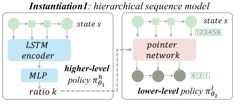
Figure 3: The instantiation of HEM.

5.2.3 Instantiation of the policy network

For the higher-level policy, we first model the higher-level policy as a tanh-Gaussian, i.e., a Gaussian distribution with an invertible squashing function ($\tanh$), which is commonly used in deep reinforcement learning [47, 48]. The mean and variance of the Gaussian are given by neural networks. The support of the tanh-Gaussian is $[-1,1]$, but a ratio of selected cuts should belong to $[0,1]$. Thus, we further perform a linear transformation on the tanh-Gaussian. Specifically, we define the parameterized higher-level policy by $\pi^{h}_{\theta_{1}}(\cdot|s)=0.5*\tanh{(K)}+0.5$, where $K\sim\mathcal{N}(\mu_{\theta_{1}}(s),\sigma_{\theta_{1}}(s))$. Since the sequence lengths of states are variable across different instances (MILPs), we use a long-short term memory (LSTM) [49] network to embed the sequence of candidate cuts. We then use a multi-layer perceptron (MLP) [50] to predict the mean and variance from the last hidden state of the LSTM.

For the lower-level policy, we formulate it as a Seq2Seq model. That is, its input is a sequence of candidate cuts, and its output is the probability distribution over ordered subsets of candidate cuts with the cardinality determined by the higher-level policy. Specifically, given a state action pair $(s,k,a_{k})$, the Seq2Seq model computes the conditional probability $\pi^{l}_{\theta_{2}}(a_{k}|s,k)$ using a parametric model to estimate the terms of the probability chain rule, i.e., $\pi^{l}_{\theta_{2}}(a_{k}|s,k)=\prod_{i=1}^{m}p_{\theta_{2}}(a_{k}^{i}|a_{k}^{1},\dots,a_{k}^{i-1},s,k)$. Here $s=\{s^{1},\dots,s^{N}\}$ is the input sequence, $m=\lfloor N*k\rfloor$ is the length of the output sequence, and $a_{k}=\{a_{k}^{1},\dots,a_{k}^{m}\}$ is a sequence of $m$ indices, each corresponding a position in the input sequence $s$. Such policy can be parametrized by the vanilla Seq2Seq model commonly used in machine translation [51, 52]. However, the vanilla Seq2Seq model is only applicable to learning on a single instance, as the number of candidate cuts varies on different instances. To generalize across different instances, we use a pointer network [53, 54]—which uses attention as a pointer to select a member of the input sequence as the output at each decoder step—to parametrize $\pi^{l}_{\theta_{2}}$ (see Appendix LABEL:appendix_pn_details for details).

5.3 Training: hierarchical policy gradient

For the cut selection task, we aim to find $\theta$ that maximizes the expected reward over all trajectories

$$J(\theta)=\mathbb{E}_{s\sim\mu,a_{k}\sim\pi_{\theta}(\cdot|s)}[r(s,a_{k})],$$ (3)

where $\theta=\left[\theta_{1},\theta_{2}\right]$ with $\left[\theta_{1},\theta_{2}\right]$ denoting the concatenation of the two vectors, $\pi_{\theta}(a_{k}|s)=\mathbb{E}_{k\sim\pi^{h}_{\theta_{1}}(\cdot|s)}[\pi^{l}_{\theta_{2}}(a_{k}|s,k)]$, and $\mu$ denotes the initial state distribution. Here we focus on training cut selection policies under the one round setting. We defer discussion on training policies under the multiple rounds setting to Section 6. To train the policy with a hierarchical structure, we derive a hierarchical policy gradient following the well-known policy gradient theorem [55, 46].

Proposition 1.

Given the cut selection policy $\pi_{\theta}(a_{k}|s)=\mathbb{E}_{k\sim\pi^{h}_{\theta_{1}}(\cdot|s)}[\pi^{l}_{\theta_{2}}(a_{k}|s,k)]$ and the training objective (3), the hierarchical policy gradient takes the form of

$$\nabla_{\theta_{1}}J(\left[\theta_{1},\theta_{2}\right])$$

$$=\mathbb{E}_{s\sim\mu,k\sim\pi^{h}_{\theta_{1}}(\cdot|s)}[\nabla_{\theta_{1}}\log(\pi^{h}_{\theta_{1}}(k|s))\mathbb{E}_{a_{k}\sim\pi^{l}_{\theta 2}(\cdot|s,k)}[r(s,a_{k})]],$$

$$\nabla_{\theta_{2}}J(\left[\theta_{1},\theta_{2}\right])$$

$$=\mathbb{E}_{s\sim\mu,k\sim\pi^{h}_{\theta_{1}}(\cdot|s),a_{k}\sim\pi^{l}_{\theta_{2}}(\cdot|s,k)}[\nabla_{\theta_{2}}\log\pi^{l}_{\theta_{2}}(a_{k}|s,k)r(s,a_{k})].$$

We provide detailed proof in Appendix A.1. We use the derived hierarchical policy gradient to update the parameters of the higher-level and lower-level policies. We implement the training algorithm in a parallel manner that is closely related to the asynchronous advantage actor-critic (A3C) [56]. Furthermore, we summarize the procedure of the training algorithm in Algorithm 1.

Algorithm 1 Pseudo code for training HEM

.

1:  Initialize Hierarchical sequence model $\pi_{[\theta_{1},\theta_{2}]}$, MILP instances $\mathcal{D}$, training dataset $\mathcal{D}_{\text{train}}$, batch size $N_{b}$, training epochs $N_{e}$, policy learning rate $\alpha$

2:  for $N_{e}$ epochs do

3:     Empty the training dataset $\mathcal{D}_{\text{train}}$

4:     for $N_{b}$ steps do

5:        Randomly sample a MILP $s_{0}$ from $\mathcal{D}$

6:        Take action $k$ and $a_{k}$ at state $s_{0}$ with the policy $\pi$

7:        Receive reward $r$ and add $(s_{0},k,a_{k},r)$ to $\mathcal{D}_{\text{train}}$

8:     end for

9:     Compute hierarchical policy gradient using $\mathcal{D}_{\text{train}}$ as in proposition 1

10:     Update the parameters, $\theta_{1}=\theta_{1}+\alpha\nabla_{\theta_{1}}J(\left[\theta_{1},\theta_{2}\right])$, $\theta_{2}=\theta_{2}+\alpha\nabla_{\theta_{2}}J(\left[\theta_{1},\theta_{2}\right])$

11:  end for

6 HEM++: Further Improvements of HEM

To further enhance HEM, we propose its improvements in terms of the formulation, policy, and training method, respectively. We denote the enhanced method of HEM by HEM++. We present the details as follows.

6.1 RL formulation

In this part, we extend the RL formulation mentioned in Section 5.1 to the multiple rounds setting by redefining the action space and the hierarchical cut selection policy. The details are as follows. Under the multiple rounds setting, we formulate the cut selection as a Markov decision process. However, this entails the challenge of computing the hierarchical policy gradient, as the hierarchical cut selection policy is defined by an expectation. To address this challenge, we redefine the action space $\mathcal{A}^{\text{ext}}$ by $[0,1]\times\mathcal{A}$, and the hierarchical cut selection policy by $\pi(k,a_{k}|s)=\pi^{h}(k|s)\cdot\pi^{l}(a_{k}|s,k)$. We present the derivation of the hierarchical policy gradient under the multiple rounds setting as follows.

Under the multiple rounds setting, we aim to find $\theta$ that maximizes the expected discounted cumulative rewards

$$J(\theta)=\mathbb{E}_{s_{0},k_{0},a_{0}^{k}\dots}[\sum_{t=0}^{\infty}\gamma^{t}r(s_{t},k_{t},a_{t}^{k})],$$ (4)

where $s_{0}\sim\mu$, $(k_{t},a_{t}^{k})\sim\pi_{\theta}(\cdot|s_{t})$, $s_{t+1}=f(s_{t},a_{t})$, $\pi_{\theta}(k_{t},a_{t}^{k}|s_{t})=\pi^{h}_{\theta_{1}}(k_{t}|s_{t})\cdot\pi^{l}_{\theta_{2}}(a_{t}^{k}|s_{t},k_{t})$, and $\gamma\in(0,1]$ is the discount factor. Then we derive a hierarchical policy gradient under the multiple rounds setting as follows.

Proposition 2.

Given the cut selection policy $\pi_{\theta}(k,a^{k}|s)=\pi^{h}_{\theta_{1}}(k|s)\cdot\pi^{l}_{\theta_{2}}(a^{k}|s,k)$ and the training objective (4), the hierarchical policy gradient takes the form of

$$\nabla_{\theta_{1}}J(\left[\theta_{1},\theta_{2}\right])$$

$$=\mathbb{E}_{s\sim\rho^{\pi_{\theta}},(k,a^{k})\sim\pi_{\theta}(\cdot|s)}[Q^{\pi_{\theta}}(s,(k,a^{k}))\nabla_{\theta_{1}}\log(\pi^{h}_{\theta_{1}}(k|s))],$$

$$\nabla_{\theta_{2}}J(\left[\theta_{1},\theta_{2}\right])$$

$$=\mathbb{E}_{s\sim\rho^{\pi_{\theta}},(k,a^{k})\sim\pi_{\theta}(\cdot|s)}[Q^{\pi_{\theta}}(s,(k,a^{k}))\nabla_{\theta_{2}}\log(\pi^{l}_{\theta_{2}}(a^{k}|s,k))],$$

where $\rho^{\pi_{\theta}}(s)=\sum_{t=0}^{\infty}\gamma^{t}P(s_{t}=s|\pi_{\theta})$ denotes the expected state visitation frequencies under the policy $\pi_{\theta}$, and $Q^{\pi_{\theta}}(s,(k,a^{k}))=\mathbb{E}_{s_{0},k_{0},a_{0}^{k},\dots}[\sum_{t=0}^{\infty}r(s_{t},k_{t},a_{t}^{k})|s_{0}=s,k_{0}=k,a_{0}^{k}=a^{k}]$ denotes the Q-value function. Due to limited space, we defer detailed derivations to Appendix A.2.

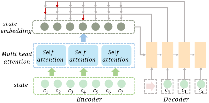
Figure 4: We instantiate the Set2Seq model via a multi-head attention encoder and a pointer decoder.

6.2 Policy network: Set to Sequence model

In this part, we formulate the lower-level model of HEM++ as a Set to Sequence (Set2Seq) model to improve the representation of input cuts by learning their order-independent embeddings. The details are as follows. As shown in Fig 3, we instantiate the lower-level model by a pointer network [53] (Seq2Seq model). The pointer network uses an LSTM encoder, which captures redundant order information when encoding input cuts. However, it is preferable for cut selection policies to be agnostic to the order of input cuts. The reason is that given the same instance and candidate cuts in different order, the corresponding optimal ordered subsets should be unchanged. Moreover, [22] has shown that vanilla Seq2Seq model can perform poorly when handling input sets. To learn order-independent embeddings of input cuts, we propose to formulate the lower-level model as a Set to Sequence (Set2Seq) model. Specifically, we first formulate the set of input cuts as a fully connected graph, and then propose an attention-pointer network to instantiate the Set2Seq model as shown in Fig 4. The attention-pointer network comprises a multi-head attention encoder and a pointer decoder. The multi-head attention encoder is a core component of the Transformer [52], which has been widely used in natural language processing [52][57] and computer vision [58][59].Compared to recurrent models, multi-head attention encoders can well capture representations invariant to the input order by leveraging the self-attention mechanism without the positional encoding. Please refer to Appendix D.2.1 for details of the self-attention mechanism. The pointer decoder is the same as that of the pointer network (see Appendix LABEL:appendix_pn_details for details).

6.3 Training: hierarchical proximal policy optimization

Under the one round setting, the formulation of the cut selection is simplified as a context bandit. Instead, the formulation of the cut selection is a MDP under the multiple rounds setting. The action space of the MDP increases exponentially with the number of the cut separation rounds, which entails the challenge of efficient exploration [60][61][62]. To address this challenge, we propose to leverage the proximal policy optimization (PPO) method [47], an on-policy state-of-the-art training method. It is well-known that PPO is much more sample-efficient than reinforce. To train the policy with a hierarchical structure, we derive a hierarchical proximal policy optimization (HPPO) based on the extended formulation in Section 6.1. Specifically, we denote the action space $\mathcal{A}^{\text{ppo}}$ by $[0,1]\times\mathcal{A}$, and the cut selection policy by $\pi^{\text{ppo}}(k,a_{k}|s)=\pi^{h}(k|s)\cdot\pi^{l}(a_{k}|s,k)$. We further denote the parameterized policy by $\pi^{\text{ppo}}_{\theta}(k,a_{k}|s)=\pi^{h}_{\theta_{1}}(k|s)\cdot\pi^{l}_{\theta_{2}}(a_{k}|s,k)$, where $\theta=\left[\theta_{1},\theta_{2}\right]$. We then derive the HPPO as follows. We denote the probability ratio of the current policies and old policies by

$$r(\theta)=\frac{\pi^{\text{ppo}}_{\theta}(k,a_{k}|s)}{\pi^{\text{ppo}}_{\theta_{\text{old}}}(k,a_{k}|s)}=\frac{\pi^{h}_{\theta_{1}}(k|s)\cdot\pi^{l}_{\theta_{2}}(a_{k}|s,k)}{\pi^{h}_{\theta_{\text{old}1}}(k|s)\cdot\pi^{l}_{\theta_{\text{old}2}}(a_{k}|s,k)}.$$ (5)

HPPO clips the ratio $r(\theta)$ to avoid destructively large policy updates following [47], i.e.,

$$r_{\epsilon}^{\text{clip}}(\theta)=\begin{cases}1+\epsilon,&\hat{A}>0\text{ and }r(\theta)\geq 1+\epsilon;\\ 1-\epsilon,&\hat{A}<0\text{ and }r(\theta)\leq 1-\epsilon;\\ r(\theta),&\text{otherwise}.\end{cases}$$ (6)

Here $\epsilon$ is a hyperparameter, and $\hat{A}$ is an estimator of the advantage function [46]. Then, we aim to find $\theta$ that maximizes the following objective:

$$J(\theta)=\mathbb{E}_{t}\left[r_{\epsilon}^{\text{clip}}(\theta)\hat{A}\right].$$ (7)

Here $\mathbb{E}_{t}[\cdot]=\mathbb{E}_{s\sim\rho^{\pi_{\theta_{\text{old}}}},(k,a_{k})\sim\pi_{\theta_{\text{old}}}}[\cdot]$, and $\rho^{\pi_{\theta_{\text{old}}}}$ denotes the expected state visitation frequencies under the policy $\pi_{\theta_{\text{old}}}$. Then, the hierarchical policy gradient takes the form of

$$\nabla_{\theta_{1}}J\left[\theta_{1},\theta_{2}\right] =\mathbb{E}_{t}[\frac{\pi^{l}_{\theta_{2}}(a_{k}|s,k)\cdot\nabla_{\theta_{1}}\pi^{h}_{\theta_{1}}(k|s)}{\pi^{h}_{\theta_{\text{old}1}}(k|s)\cdot\pi^{l}_{\theta_{\text{old}2}}(a_{k}|s,k)}\hat{A}],$$ (8)

$$\nabla_{\theta_{2}}J\left[\theta_{1},\theta_{2}\right] =\mathbb{E}_{t}[\frac{\pi^{h}_{\theta_{1}}(k|s)\cdot\nabla_{\theta_{2}}\pi^{l}_{\theta_{2}}(a_{k}|s,k)}{\pi^{h}_{\theta_{\text{old}1}}(k|s)\cdot\pi^{l}_{\theta_{\text{old}2}}(a_{k}|s,k)}\hat{A}],$$ (9)

where $\hat{A}\leq 0$ and $r(\theta)\geq 1-\epsilon$ or $\hat{A}\geq 0$ and $r(\theta)\leq 1+\epsilon$. Please refer to Appendix D.2.2 for details of estimating the advantage function $\hat{A}$ and the implementation of HPPO.

6.4 Discussion on advantages of HEM/HEM++

We discuss some additional advantages of HEM/HEM++ as follows. (1) Inspired by hierarchical reinforcement learning [63, 64], HEM/HEM++ leverages the hierarchical structure of the cut selection task, which is important for efficient exploration in complex decision-making tasks. (2) Previous methods [19, 21] usually train cut selection policies via black-box optimization methods such as evolution strategies [65]. In contrast, HEM/HEM++ is differentiable and we train the HEM/HEM++ via gradient-based algorithms, which is more sample efficient than black-box optimization methods [46, 66]. Although we can offline generate training samples as much as possible using a MILP solver, high sample efficiency is significant as generating samples can be extremely time-consuming in practice.

6.5 Theoretical Analysis

We provide analysis to establish theoretical performance guarantees for HEM/HEM++ in this part.

We show that the cutting plane algorithm with our proposed HEM/HEM++ selecting cuts finds optimal solutions of Integer Linear Programs in a finite number of iterations under some mild assumptions. We provide a detailed analysis as follows. Specifically, we focus on a pure cutting plane algorithm for solving Integer Linear Programs (ILP), which follows previous work [67, 68]. We focus on the ILPs under the assumption that the objective function is defined by a positive integer vector and the feasible region is bounded. Specifically, the ILP takes the form of

$$\max_{\mathbf{x}}\{\mathbf{c}^{\top}\mathbf{x}:\mathbf{x}\in\mathbb{P}\cap\mathbb{Z}^{n}\}$$ (10)

, where $\mathbf{c}\in\mathbb{Z}^{n}_{+}$ and $\mathbb{P}$ denotes a bounded polyhedron in $\left[0,d\right]^{n}$ with $d$ being some positive integer. We assume that $\mathbb{P}\cap\mathbb{Z}^{n}$ is nonempty, i.e., $\mathbb{P}$ contains at least one integral point.

Definition 1.

(Lexicographically Lower) Given two vectors $\mathbf{x},\mathbf{y}\in\mathbb{R}^{n+1}$, the vector $\mathbf{x}=(x_{0},\dots,x_{n})$ is defined to be lexicographically lower than the vector $\mathbf{y}=(y_{0},\dots,y_{n})$ if there exists an integer $k\in\{0,\dots,n\}$ with $x_{k}<y_{k}$ and $x_{i}=y_{i}$ for all $i<k$. We write $\mathbf{x}<_{L}\mathbf{y}$. And similarly, we write $\mathbf{x}\leq_{L}\mathbf{y}$ if $\mathbf{x}<_{L}\mathbf{y}$ or $\mathbf{x}=\mathbf{y}$.

For simplicity, we write the objective in (10) as a lexicographic optimization problem [69], taking the form of

$$\text{lexmax}\{z_{0},z_{1},\dots,z_{n}:\mathbf{z}\in\mathbb{S}\},$$ (11)

where $z_{0}=\mathbf{c}^{\top}\mathbf{x}$, $z_{i}=x_{i},\forall i\in\{1,\dots,n\}$ and $\mathbb{S}=\mathbb{Z}\times(\mathbb{P}\cap\mathbb{Z}^{n})$. The lexicographic optimization objective in (11) aims to find a lexicographically maximum vector in $\mathbb{S}$. We define the linear programming (LP) relaxation of the problem (11) by

$$\text{lexmax}\{z_{0},z_{1},\dots,z_{n}:\mathbf{z}\in\mathbb{S}^{\prime}\},$$ (12)

where $\mathbb{S}^{\prime}=\mathbb{R}\times\mathbb{P}$.

Following [67], we focus on the following cutting planes.

Proposition 3.

(Cutting Planes) Let $\mathbf{z}=(z_{0},z_{1},\dots,z_{n})\in\mathbb{R}\times\left[0,d\right]^{n}$. Then the following linear inequalities are satisfied by any integer vector $\mathbf{x}\in\mathbb{Z}\times(\left[0,d\right]\cap\mathbb{Z})^{n}$ which is lexicographically lower than $\mathbf{z}$ (i.e., $\mathbf{x}\leq_{L}\mathbf{z}$)

$$x_{i}+\sum_{j=0}^{i-1}a_{i-j}(x_{j}-\lceil z_{j}\rceil)\leq\lfloor z_{i}\rfloor$$ (13)

for all $i\in\{0,\dots,n\}$ with $a_{1}=d$ and $a_{k}=d(1+\sum_{j=1}^{k-1}a_{j})$ for any integer $k\in\{2,\dots,n\}$, and $\sum_{j=0}^{-1}a_{0}(x_{0}-\lceil z_{0}\rceil)=0$.

We defer detailed proof of Proposition 3 to Appendix A.3. We denote the inequality (13) with some particular index value $i\in\{0,\dots,n\}$ by (13)_i. Thus, we can generate $n+1$ cutting planes according to the inequalities (13).

The cutting plane algorithm with HEM/HEM++ starts with solving the LP relaxation of (11) (i.e., the problem (12)). Then we generate $n+1$ cutting planes according to (13), and HEM/HEM++ select a cut to be added to the LP relaxation. Then the procedure proceeds to the next iteration by solving the new LP relaxation. Finally, the algorithm is iterated until the optimal integer solution is found. We show that the cutting plane algorithm with HEM/HEM++ selecting cuts finds optimal integer solutions of the ILPs in a finite number of iterations under the following mild assumption.

Assumption 1.

HEM/HEM++ learns a cut selection policy to select the $k$-th cut at each iteration. Note that $k=\text{argmin}_{j}\{z_{j}^{*}\not\in\mathbb{Z},j=0,\dots,n\}$, where $\mathbf{z}_{t}^{\star}=(z_{0}^{*},z_{1}^{*},\dots,z_{n}^{*})$ denotes the optimal solution of the LP relaxation at iteration $t$.

Theorem 1.

With the cutting planes in Proposition 3 and under the Assumption 1, the cutting plane algorithm with HEM/HEM++ selecting cuts finds an optimal solution of the ILP (11) in a finite number of iterations.

We defer detailed proof to Appendix A.4.

Algorithm 2 Pseudo code for extracting order rules from hierarchical sequence model

.

1:  Input Hierarchical sequence model $\pi_{[\theta_{1},\theta_{2}]}$, MILP training dataset $\mathcal{D}_{\text{train}}$

2:  Input Top-3 cutting plane category counters $\mathcal{C}_{1},\mathcal{C}_{2},\mathcal{C}_{3}=\{0\}$, cutting plane categories $\mathcal{K}$

3:  for each instance $\mathcal{D}_{i}$ in $\mathcal{D}_{\text{train}}$ do

4:     Solve $\mathcal{D}_{i}$ with HEM selecting cuts

5:     Record the order of categories of selected cuts

6:     Record the top-3 categories in the order, and find their corresponding indexes in $\mathcal{K}$, i.e., $i,j,k$.

7:     Increase the counters: $\mathcal{C}_{1i}+=1$, $\mathcal{C}_{2j}+=1$, $\mathcal{C}_{3k}+=1$

8:  end for

9:  Find the maximum counter indexes: $i_{\text{top1}}=\text{argmax}(\mathcal{C}_{1})$, $i_{\text{top2}}=\text{argmax}(\mathcal{C}_{2})$, $i_{\text{top3}}=\text{argmax}(\mathcal{C}_{3})$

10:  Return the top-3 categories, i.e., $\mathcal{K}_{i_{\text{top1}}}$, $\mathcal{K}_{i_{\text{top2}}}$, $\mathcal{K}_{i_{\text{top3}}}$

TABLE I: Statistical description of used datasets. In all datasets, $m$ denotes the average number of constraints and $n$ denotes the average number of variables. NCuts denotes the number of generated candidate cuts. Inference Time denotes the inference time of our proposed HEM given the average number of candidate cuts.

Datasets	Set Covering	Maximum Independent Set	Multiple Knapsack	MIK	CORLAT	Load Balancing	Anonymous	MIPLIB mixed neos	MIPLIB mixed supportcase
$m$	500	1953	72	346	486	64304	49603	5660	19910
$n$	1000	500	720	413	466	61000	37881	6958	19766
NCuts Avg (stdev)	780.51 (290)	57.04 (16)	45.00 (13)	62.00 (13)	60.00 (33)	392.53 (33)	79.40 (73)	239.00 (154)	173.25 (267)
Inference Time (s)	1.58	0.11	0.09	0.12	0.12	0.77	0.15	0.47	0.34

7 Extracting Order Rules from HEM

To enhance modern MILP solvers, we can directly deploy our HEM to MILP solvers to improve their efficiency. In addition, we can also extract more effective heuristic rules than manually-designed heuristics from learned policies to facilitate the deployment of HEM. Extracting rules from HEM leads to two major advantages. First, the extracted rules are well readable for human experts, and thus easy to debug. Second, we can deploy the extracted rules to purely CPU-based environments, which are applicable to the common solver deployment environments, i.e., the CPU computing-intensive environments. However, it is challenging to directly extract the cut selection rules from HEM. As it involves three problems (i.e., (P1)-(P3)) that are very complex, it is difficult to extract general cut selection rules from HEM. Furthermore, existing heuristics aim to tackle (P1)-(P2) but neglect the importance of tackling (P3). Therefore, we propose to extract order rules for tackling (P3) to enhance existing manually-designed heuristics.

Specifically, we record the order of categories of selected cuts for each instance. For generality, we aim to extract instance-independent order rules rather than instance-dependent. To this end, we count the number of times that each cutting plane category is located at the k-th ($k=1,2,3,\dots$) position in the order across all instances. Then we record the cutting plane category with the highest number of times that is located at the k-th ($k=1,2,3,\dots$) position, respectively. Finally, we increase the priority of the cut generators according to the order of cutting plane categories. We denote the default heuristics in MILP solvers with extracted order rules by Default+. We summarize the procedure of extracting order rules from HEM in Algorithm 2. Please refer to Section 8.7.2 for the evaluation of Default+.

8 Experiments

Our experiments have six main parts. (1) We evaluate HEM on three classical MILP problems and six challenging MILP problem benchmarks from diverse application areas (see Section 8.2). (2) We evaluate whether HEM++ improves HEM (see Section 8.3). (3) We perform carefully designed ablation studies to provide further insight into HEM (see Section 8.4). (4) We test whether HEM can generalize to instances significantly larger than those seen during training (see Section 8.5). (5) We perform carefully designed visualization experiments and explainability analysis (see Section 8.6). (6) We deploy our approach to real-world challenging MILP problems (see Section 8.7).

8.1 Experiments setup

8.1.1 Benchmarks

We evaluate our approach on nine $\mathcal{NP}$-hard MILP problem benchmarks, which consist of three classical synthetic MILP problems and six challenging MILP problems from diverse application areas. We divide the nine problem benchmarks into three categories according to the difficulty of solving them using the SCIP 8.0.0 solver [10]. We call the three categories easy, medium, and hard datasets, respectively. (1) Easy datasets comprise three widely used synthetic MILP problem benchmarks: Set Covering [70], Maximum Independent Set [71], and Multiple Knapsack [72]. We artificially generate instances following [27, 73]. (2) Medium datasets comprise MIK [74] and CORLAT [75], which are widely used benchmarks for evaluating MILP solvers [33, 8]. (3) Hard datasets include the Load Balancing problem, inspired by large-scale systems at Google, and the Anonymous problem, inspired by a large-scale industrial application [26]. Moreover, hard datasets contain benchmarks from MIPLIB 2017 (MIPLIB) [23]. Although [15] has shown that directly learning over the full MIPLIB can be extremely challenging, we propose to learn over subsets of MIPLIB. We construct two subsets, called MIPLIB mixed neos and MIPLIB mixed supportcase. Due to limited space, please see Appendix B.3 for details of these datasets.

We summarize the statistical description of these datasets in Table I. Let $n,m$ denote the average number of variables and constraints in the MILPs. Let $m\times n$ denote the size of the MILPs. It is worth emphasizing that the maximum size of the dataset we use is two orders of magnitude larger than that used in previous work [19, 16]. Furthermore, we evaluate the average inference time of HEM given the generated cuts. The results in Table I show that the computational overhead of HEM is quite low.

TABLE II: Policy evaluation on easy, medium, and hard datasets. The best performance is marked in bold. For all datasets, the results show that HEM significantly outperforms the baselines in terms of solving time and primal-dual gap integral.

	Easy: Set Covering ($n=1000,\,\,m=500$)			Easy: Max Independent Set ($n=500,\,\,m=1953$)			Easy: Multiple Knapsack ($n=720,\,\,m=72$)
Method	Time(s) $\downarrow$	Improvement (time, %) $\uparrow$	PD integral $\downarrow$	Time(s) $\downarrow$	Improvement (time, %) $\uparrow$	PD integral $\downarrow$	Time(s) $\downarrow$	Improvement (time, %) $\uparrow$	PD integral $\downarrow$
NoCuts	6.31 (4.61)	NA	56.99 (38.89)	8.78 (6.66)	NA	71.31 (51.74)	9.88 (22.24)	NA	16.41 (14.16)
Default	4.41 (5.12)	29.90	55.63 (42.21)	3.88 (5.04)	55.80	29.44 (35.27)	9.90 (22.24)	-0.20	16.46 (14.25)
Random	5.74 (5.19)	8.90	67.08 (46.58)	6.50 (7.09)	26.00	52.46 (53.10)	13.10 (35.51)	-32.60	20.00 (25.14)
NV	9.86 (5.43)	-56.50	99.77 (53.12)	7.84 (5.54)	10.70	61.60 (43.95)	13.04 (36.91)	-32.00	21.75 (24.71)
Eff	9.65 (5.45)	-53.20	95.66 (51.71)	7.80 (5.11)	11.10	61.04 (41.88)	9.99 (19.02)	-1.10	20.49 (22.11)
SBP	1.91 (0.36)	69.60	38.96 (8.66)	2.43 (5.55)	72.30	21.99 (40.86)	7.74 (12.36)	21.60	16.45 (16.62)
HEM (Ours)	1.85 (0.31)	70.60	37.92 (8.46)	1.76 (3.69)	80.00	16.01 (26.21)	6.13 (9.61)	38.00	13.63 (9.63)

	Medium: MIK ($n=413,\,\,m=346$)			Medium: Corlat ($n=466,\,\,m=486$)			Hard: Load Balancing ($n=61000,\,\,m=64304$)
Method	Time(s) $\downarrow$	PD integral $\downarrow$	Improvement $\uparrow$ (PD integral, %)	Time(s) $\downarrow$	PD integral $\downarrow$	Improvement $\uparrow$ (PD integral, %)	Time(s) $\downarrow$	PD integral $\downarrow$	Improvement $\uparrow$ (PD integral, %)
NoCuts	300.01 (0.009)	2355.87 (996.08)	NA	103.30 (128.14)	2818.40 (5908.31)	NA	300.00 (0.12)	14853.77 (951.42)	NA
Default	179.62 (122.36)	844.40 (924.30)	64.10	75.20 (120.30)	2412.09 (5892.88)	14.40	300.00 (0.06)	9589.19 (1012.95)	35.40
Random	289.86 (28.90)	2036.80 (933.17)	13.50	84.18 (124.34)	2501.98 (6031.43)	11.20	300.00 (0.09)	13621.20 (1162.02)	8.30
NV	299.76 (1.32)	2542.67 ( 529.49)	-7.90	90.26 (128.33)	3075.70 (7029.55)	-9.10	300.00 (0.05)	13933.88 (971.10)	6.20
Eff	298.48 (5.84)	2416.57 (642.41)	-2.60	104.38 (131.61)	3155.03 (7039.99)	-11.90	300.00 (0.07)	13913.07 (969.95)	6.30
SBP	286.07 (41.81)	2053.30 (740.11)	12.80	70.41 (122.17)	2023.87 (5085.96)	28.20	300.00 (0.10)	12535.30 (741.43)	15.60
HEM(Ours)	176.12 (125.18)	785.04 (790.38)	66.70	58.31 (110.51)	1079.99 (2653.14)	61.68	300.00 (0.04)	9496.42 (1018.35)	36.10

	Hard: Anonymous ($n=37881,\,\,m=49603$)			Hard: MIPLIB mixed neos ($n=6958,\,\,m=5660$)			Hard: MIPLIB mixed supportcase ($n=19766,\,\,m=19910$)
Method	Time(s) $\downarrow$	PD integral $\downarrow$	Improvement $\uparrow$ (PD integral, %)	Time(s) $\downarrow$	PD integral $\downarrow$	Improvement $\uparrow$ (PD integral, %)	Time(s) $\downarrow$	PD integral $\downarrow$	Improvement $\uparrow$ (PD integral, %)
NoCuts	246.22 (94.90)	18297.30 (9769.42)	NA	253.65 (80.29)	14652.29 (12523.37)	NA	170.00 (131.60)	9927.96 (11334.07)	NA
Default	244.02 (97.72)	17407.01 (9736.19)	4.90	256.58 (76.05)	14444.05 (12347.09)	1.42	164.61 (135.82)	9672.34 (10668.24)	2.57
Random	243.49 (98.21)	16850.89 (10227.87)	7.80	255.88 (76.65)	14006.48 (12698.76)	4.41	165.88 (134.40)	10034.70 (11052.73)	-1.07
NV	242.01 (98.68)	16873.66 (9711.16)	7.80	263.81 (64.10)	14379.05 (12306.35)	1.86	161.67 (131.43)	8967.00 (9690.30)	9.68
Eff	244.94 (93.47)	17137.87 (9456.34)	6.30	260.53 (68.54)	14021.74 (12859.41)	4.30	167.35 (134.99)	9941.55 (10943.48)	-0.14
SBP	245.71 (92.46)	18188.63 (9651.85)	0.59	256.48 (78.59)	13531.00 (12898.22)	7.65	165.61 (135.25)	7408.65 (7903.47)	25.37
HEM(Ours)	241.68 (97.23)	16077.15 (9108.21)	12.10	248.66 (89.46)	8678.76 (12337.00)	40.77	162.96 (138.21)	6874.80 (6729.97)	30.75

8.1.2 Implementation details

Throughout all experiments, we use SCIP 8.0.0 [10] as the backend solver, which is the state-of-the-art open source solver, and is widely used in research of machine learning for combinatorial optimization [27, 21, 15, 8]. Following [27, 21, 16], we only allow cutting plane generation and selection at the root node. Throughout all experiments, we set the cut separation rounds as one unless otherwise specified. We keep all the other SCIP parameters to default so as to make comparisons as fair and reproducible as possible. We emphasize that all of the SCIP solver’s advanced features, such as presolve and heuristics, are open, which ensures that our setup is consistent with the practice setting. Throughout all experiments, we set the solving time limit as 300 seconds. For completeness, we also evaluate HEM with a much longer time limit of three hours. The results are given in Appendix E.4. We train HEM with ADAM [76] using the PyTorch [77]. Additionally, we also provide another implementation using the MindSpore [78]. For simplicity, we split each dataset into the train and test sets with $80\%$ and $20\%$ instances. To further improve HEM, one can construct a valid set for hyperparameters tuning. We train our model on the train set, and select the best model on the train set to evaluate on the test set. Please refer to Appendix D.1 for implementation details, hyperparameters, and hardware specification.

8.1.3 Main Baselines

Our main baselines include five widely-used human-designed cut selection rules and a state-of-the-art (SOTA) learning-based method. Cut selection rules include NoCuts, Random, Normalized Violation (NV), Efficacy (Eff), and Default. NoCuts does not add any cuts. Default denotes the default rules used in SCIP 8.0.0. For learning-based methods, we implement a SOTA learning-based method [19], namely score-based policy (SBP), as our main learning baseline. All baselines, except Default and NoCuts, select a fixed ratio of candidate cuts with high scores. Please see Appendix D.4.1 for implementation details of these baselines.

8.1.4 Evaluation metrics

We use two widely used evaluation metrics, i.e., the average solving time (Time, lower is better), and the average primal-dual gap integral (PD integral, lower is better). Additionally, we provide more results in terms of another two metrics, i.e., the average number of nodes and the average primal-dual gap, in Appendix C.1. Furthermore, to evaluate different cut selection methods compared to pure branch-and-bound without cutting plane separation, we propose an Improvement metric. Specifically, we define the metric by $\text{Im}_{M}(\cdot)=\frac{M(\text{NoCuts})-M(\cdot)}{M(\text{NoCuts})},$ where $M(\text{NoCuts})$ represents the performance of NoCuts, and $M(\cdot)$ represents a mapping from a method to its performance. The improvement metric represents the improvement of a given method compared to NoCuts. We mainly focus on the Time metric on the easy datasets, as the solver can solve all instances to optimality within the given time limit. However, HEM and the baselines cannot solve all instances to optimality within the time limit on the medium and hard datasets. As a result, the average solving time of those unsolved instances is the same, which makes it difficult to distinguish the performance of different cut selection methods using the Time metric. Therefore, we mainly focus on the PD integral metric on the medium and hard datasets. The PD integral is also a well-recognized metric for evaluating the solver performance [26, 41].

8.2 Comparative evaluation of HEM

The results in Table II suggest the following. (1) Easy datasets. HEM significantly outperforms all the baselines on the easy datasets, especially on Maximum Independent Set and Multiple Knapsack. SBP achieves much better performance than all the rule-based baselines, demonstrating that our implemented SBP is a strong baseline. Compared to SBP, HEM improves the Time by up to $16.4\%$ on the three datasets, demonstrating the superiority of our method over the SOTA learning-based method. (2) Medium datasets. On MIK and CORLAT, HEM still outperforms all the baselines. Especially on CORLAT, HEM achieves at least $33.48\%$ improvement in terms of the PD integral compared to the baselines. (3) Hard datasets. HEM significantly outperforms the baselines in terms of the PD integral on several problems in the hard datasets. HEM achieves outstanding performance on two challenging datasets from MIPLIB 2017 and real-world problems (Load Balancing and Anonymous), demonstrating the powerful ability to enhance MILP solvers with HEM in large-scale real-world applications. Moreover, SBP performs extremely poorly on several medium and hard datasets, which implies that it can be difficult to learn good cut selection policies on challenging MILP problems.

TABLE III: Comparison with two more learning baselines, i.e., AdaptiveCutsel [15] and Lookahead [16], on Maximum Independent Set, CORLAT, and MIPLIB mixed supportcase. The best performance is marked in bold.

	Easy: Maximum Independent Set ($n=500,\,\,m=1953$)			Medium: CORLAT ($n=466,\,\,m=486$)			Hard: MIPLIB mixed supportcase ($n=19766,\,\,m=19910$)
Method	Time(s) $\downarrow$	Improvement $\uparrow$ (Time, %)	PD integral $\downarrow$	Time(s) $\downarrow$	PD integral $\downarrow$	Improvement $\uparrow$ (PD integral, %)	Time(s) $\downarrow$	PD integral $\downarrow$	Improvement $\uparrow$ (PD integral, %)
NoCuts	8.78 (6.66)	NA	71.31 (51.74)	103.31 (128.14)	2818.41 (5908.31)	NA	170.00 (131.60)	9927.96 (11334.07)	NA
Default	3.88 (5.04)	55.80	29.44 (35.27)	75.21 (120.30)	2412.09 (5892.88)	14.42	164.61 (135.82)	9672.34 (10668.24)	2.57
AdaptiveCutsel	2.74 (3.92)	68.79	21.40 (27.95)	74.61 (120.74)	1619.50 (3862.10)	42.54	161.03 (136.40)	8769.63 (10008.97)	11.67
Lookahead	2.27 (5.00)	74.15	20.89 (37.38)	74.38 (125.47)	1493.00 (3684.44)	47.03	159.61 (130.97)	9293.82 (10428.78)	6.39
SBP	2.43 (5.55)	72.30	21.99 (40.86)	70.42 (122.17)	2023.87 (5085.96)	28.19	165.61 (135.25)	7408.65 (7903.47)	25.37
HEM (Ours)	1.76 (3.69)	80.00	16.01 (26.21)	58.31 (110.51)	1079.99 (2653.14)	61.68	162.96 (138.21)	6874.80 (6729.97)	30.75

TABLE IV: The average performance of HEM++ and the baselines in the multiple rounds setting on Maximum Independent Set, CORLAT, and MIPLIB mixed supportcase. The best performance is marked in bold.

	Easy: Maximum Independent Set ($n=500,\,\,m=1953$)			Medium: CORLAT ($n=466,\,\,m=486$)			Hard: MIPLIB mixed supportcase ($n=19766,\,\,m=19910$)
Method	Time (s) $\downarrow$	Improvement $\uparrow$ (Time, %)	PD integral $\downarrow$	Time (s) $\downarrow$	PD integral $\downarrow$	Improvement $\uparrow$ (PD integral, %)	Time (s) $\downarrow$	PD integral $\downarrow$	Improvement $\uparrow$ (PD integral, %)
NoCuts	8.78 (6.66)	NA	71.32 (51.74)	103.31 (128.14)	2818.41 (5908.31)	NA	170.00 (131.60)	9927.96 (11334.07)	NA
Default	0.28 (0.09)	96.78	6.43 (1.17)	18.19 (63.09)	1293.01 (4988.62)	54.12	149.40 (135.06)	8273.98 (8854.58)	16.66
Random	1.01 (2.38)	88.53	10.91 (12.28)	21.45 (63.13)	1537.53 (4990.91)	45.45	153.20 (136.38)	8407.73 (9667.58)	15.31
NV	1.24 (1.62)	85.91	12.38 (8.63)	77.21 (119.69)	3083.72 (7544.76)	-9.41	156.46 (130.11)	8934.07 (10299.78)	10.01
Eff	0.27 (0.09)	96.97	6.39 (1.11)	23.12 (70.35)	2305.60 (7032.43)	18.20	128.88 (126.15)	7368.99 (8642.19)	25.77
SBP	0.26 (0.14)	97.04	6.57 (1.70)	8.93 (35.76)	692.31 (2678.17)	75.44	147.92 (131.63)	7360.16 (7782.50)	25.86
HEM++ (Ours)	0.21 (0.09)	97.63	6.03 (1.12)	4.96 (10.08)	460.68 (980.31)	83.65	141.71 (133.49)	6545.59 (7241.17)	34.07

TABLE V: Evaluation of HEM++ on three extremely hard datasets under the one round setting. The best performance is marked in bold. The results show that HEM++ outperforms HEM in terms of the primal-dual gap integral.

	Hard: Anonymous ($n=37881,\,\,m=49603$)			Hard: MIPLIB mixed neos ($n=6958,\,\,m=5660$)			Hard: MIPLIB mixed supportcase ($n=19766,\,\,m=19910$)
Method	Time (s) $\downarrow$	PD integral $\downarrow$	Improvement $\uparrow$ (%, PD integral)	Time (s) $\downarrow$	PD integral $\downarrow$	Improvement $\uparrow$ (%, PD integral)	Time (s) $\downarrow$	PD integral $\downarrow$	Improvement $\uparrow$ (%, PD integral)
NoCuts	246.22 (94.90)	18297.30 (9769.42)	NA	253.65 (80.29)	14652.29 (12523.37)	NA	170.00 (131.60)	9927.96 (11334.07)	NA
Default	244.02 (97.72)	17407.01 (9736.19)	4.90	256.58 (76.05)	14444.05 (12347.09)	1.42	164.61 (135.82)	9672.34 (10668.24)	2.57
SBP	245.71 (92.46)	18188.63 (9651.85)	0.59	256.48 (78.59)	13531.00 (12898.22)	7.65	165.61 (135.25)	7408.65 (7903.47)	25.37
HEM (Ours)	241.68 (97.23)	16077.15 (9108.21)	12.10	248.66 (89.46)	8678.76 (12337.00)	40.77	162.96 (138.21)	6874.80 (6729.97)	30.75
HEM++ (Ours)	243.23 (96.62)	15444.70 (9260.60)	15.59	252.07 (83.06)	8557.46 (12395.07)	41.60	153.83 (131.55)	6586.04 (6313.25)	33.66

8.2.1 Comparison with more learning baselines

To fully evaluate the superiority of HEM, we compare HEM with two more learning baselines, i.e., AdaptiveCutsel [15] and Lookahead [16]. As shown in Table III, the results demonstrate that HEM significantly outperforms the two learning-based methods by a large margin in terms of the Time (up to 11.21% improvement) and PD integral (up to 24.36% improvement). Both SBP and Lookahead significantly outperform the default heuristic, showing that learning cut selection is important for improving solver performance. Moreover, SBP performs on par with Lookahead on easy and medium datasets (Maximum Independent Set and CORLAT), while SBP outperforms Lookahead on hard datasets (MIPLIB mixed supportcase). This demonstrates that SBP is a strong learning baseline, especially on large-scale hard datasets. Therefore, we use SBP as our main learning baseline in this paper.

8.3 Comparative evaluation of HEM++

Compared with HEM, HEM++ has two main advantages. First, the formulation of HEM++ is more widely applicable. To demonstrate its superiority, we compare HEM++ with the baselines under the multiple rounds setting in Section 8.3.1. Second, the model and training method of HEM++ are more powerful. To demonstrate the effectiveness of its model and training method, we compare HEM++ with HEM under the one round setting in Section 8.3.2.

8.3.1 Evaluation under the multiple rounds setting

In this part, we compare HEM++ with the baselines rather than HEM under the multiple rounds setting, as it is challenging for HEM to compute multi-step policy gradient. Note that we reimplement all the baselines to adapt to the multiple rounds setting. Please refer to Appendix D.4.2 for implementation details of the baselines under the multiple rounds setting. Specifically, we set the cut separation rounds as $T=10$, and compare HEM++ with the baselines on Maximum Independent Set (Easy), CORLAT (Medium), and MIPLIB mixed supportcase (Hard). The results in Table IV show that HEM significantly outperforms the baselines in terms of the Time and/or PD integral. This demonstrates that HEM++ is well applicable to the multiple rounds setting, suggesting the superiority of HEM++ over HEM.

8.3.2 Evaluation under the one round setting

To evaluate whether our proposed HEM++ further improves the performance of HEM, we compare HEM++ with HEM under the one round setting. Specifically, we compare HEM++ with HEM on three large-scale datasets, i.e., Anonymous, MIPLIB mixed neos, and MIPLIB mixed supportcase. Please refer to Appendix C.2 for results on more datasets. The results in Tabel V show that HEM++ outperforms HEM in terms of the Time and/or PD integral, demonstrating the effectiveness of HEM++. Specifically, the results suggest that the Set2Seq model in HEM++ well improves the representation of input cuts, and the HPPO in HEM++ further improves the sample-efficiency.

8.4 Ablation study

In this subsection, we present ablation studies on Maximum Independent Set (MIS), CORLAT, and MIPLIB mixed neos, which are representative datasets from the easy, medium, and hard datasets, respectively. We provide more results on the other datasets in Appendix E.1.

TABLE VI: Comparison between HEM and HEM without the higher-level model. The best performance is marked in bold.

	Easy: Max Independent Set ($n=500,\,\,m=1953$)			Medium: Corlat ($n=466,\,\,m=486$)			Hard: MIPLIB mixed neos ($n=6958,\,\,m=5660$)
Method	Time(s) $\downarrow$	Improvement $\uparrow$ (Time, %)	PD integral $\downarrow$	Time(s) $\downarrow$	PD integral $\downarrow$	Improvement $\uparrow$ (PD integral, %)	Time(s) $\downarrow$	PD integral $\downarrow$	Improvement $\uparrow$ (PD integral, %)
NoCuts	8.78 (6.66)	NA	71.31 (51.74)	103.30 (128.14)	2818.40 (5908.31)	NA	253.65 (80.29)	14652.29 (12523.37)	NA
Default	3.88 (5.04)	55.81	29.44 (35.27)	75.20 (120.30)	2412.09 (5892.88)	14.42	256.58 (76.05)	14444.05 (12347.09)	1.42
SBP	2.43 (5.55)	72.32	21.99 (40.86)	70.41 (122.17)	2023.87 (5085.96)	28.19	256.48 (78.59)	13531.00 (12898.22)	7.65
HEM w/o H	1.88 (4.20)	78.59	16.70 (28.15)	63.14 (115.26)	1939.08 (5484.83)	31.20	249.21 (88.09)	13614.29 (12914.76)	7.08
HEM (Ours)	1.76 (3.69)	79.95	16.01 (26.21)	58.31 (110.51)	1079.99 (2653.14)	61.68	248.66 (89.46)	8678.76 (12337.00)	40.77

TABLE VII: Comparison between HEM, HEM-ratio, and HEM-ratio-order. The best performance is marked in bold.

	Easy: Maximum Independent Set ($n=500,\,\,m=1953$)			Medium: Corlat ($n=466,\,\,m=486$)			Hard: MIPLIB mixed neos ($n=6958,\,\,m=5660$)
Method	Time(s) $\downarrow$	Improvement $\uparrow$ (Time, %)	PD integral $\downarrow$	Time(s) $\downarrow$	PD integral $\downarrow$	Improvement $\uparrow$ (PD integral, %)	Time(s) $\downarrow$	PD integral $\downarrow$	Improvement $\uparrow$ (PD integral, %)
NoCuts	8.78 (6.66)	NA	71.31 (51.74)	103.30 (128.14)	2818.40 (5908.31)	NA	253.65 (80.29)	14652.29 (12523.37)	NA
Default	3.88 (5.04)	55.81	29.44 (35.27)	75.20 (120.30)	2412.09 (5892.88)	14.42	256.58 (76.05)	14444.05 (12347.09)	1.42
SBP	2.43 (5.55)	72.32	21.99 (40.86)	70.41 (122.17)	2023.87 (5085.96)	28.19	256.48 (78.59)	13531.00 (12898.22)	7.65
HEM-ratio-order	2.30 (5.18)	73.80	21.19 (38.52)	70.94 (122.93)	1416.66 (3380.10)	49.74	245.99 (93.67)	14026.75 (12683.60)	4.27
HEM-ratio	2.26 (5.06)	74.26	20.82 (37.81)	67.27 (117.01)	1251.60 (2869.87)	55.59	244.87 (95.56)	13659.93 (12900.59)	6.77
HEM (Ours)	1.76 (3.69)	79.95	16.01 (26.21)	58.31 (110.51)	1079.99 (2653.14)	61.68	248.66 (89.46)	8678.76 (12337.00)	40.77

TABLE VIII: Comparison between HEM++, HEM++ without HPPO, and HEM++ without Set2Seq.

	Hard: Anonymous ($n=37881,\,\,m=49603$)			Hard: MIPLIB mixed neos ($n=6958,\,\,m=5660$)			Hard: MIPLIB mixed supportcase ($n=19766,\,\,m=19910$)
Method	Time (s) $\downarrow$	PD integral $\downarrow$	Improvement $\uparrow$ (%, PD integral)	Time (s) $\downarrow$	PD integral $\downarrow$	Improvement $\uparrow$ (%, PD integral)	Time (s) $\downarrow$	PD integral $\downarrow$	Improvement $\uparrow$ (%, PD integral)
NoCuts	246.22 (94.90)	18297.30 (9769.42)	NA	253.65 (80.29)	14652.29 (12523.37)	NA	170.00 (131.60)	9927.96 (11334.07)	NA
Default	244.02 (97.72)	17407.01 (9736.19)	4.90	256.58 (76.05)	14444.05 (12347.09)	1.42	164.61 (135.82)	9672.34 (10668.24)	2.57
SBP	245.71 (92.46)	18188.63 (9651.85)	0.59	256.48 (78.59)	13531.00 (12898.22)	7.65	165.61 (135.25)	7408.65 (7903.47)	25.37
HEM	241.68 (97.23)	16077.15 (9108.21)	12.10	248.66 (89.46)	8678.76 (12337.00)	40.77	162.96 (138.21)	6874.80 (6729.97)	30.75
HEM++ w/o HPPO	239.50 (104.24)	15848.32 (9870.58)	13.38	254.38 (79.07)	12574.79 (12548.1)	14.18	154.66 (135.77)	8440.19 (9655.38)	14.99
HEM++ w/o Set2Seq	250.19 (87.43)	17144.41 (9084.42)	6.30	258.80 (71.41)	8627.41 (12353.81)	41.12	169.43 (132.38)	6737.99 (6518.49)	32.13
HEM++	243.23 (96.62)	15444.70 (9260.60)	15.59	252.07 (83.06)	8557.46 (12395.07)	41.60	153.83 (131.55)	6586.04 (6313.25)	33.66

TABLE IX: Evaluate the generalization ability of HEM on Set Covering and Maximum Independent Set.

	Set Covering ($n=1000,\,m=1000,\,2\times$)			Set Covering ($n=1000,\,m=2000,\,4\times$)
Method	Time(s) $\downarrow$	Improvement $\uparrow$ (time, %)	PD integral $\downarrow$	Time(s) $\downarrow$	Improvement $\uparrow$ (time, %)	PD integral $\downarrow$
NoCuts	82.69 (78.27)	NA	609.43 (524.92)	284.44 (48.70)	NA	3215.34 (1019.47)
Default	61.01 (78.12)	26.22	494.63 (545.76)	149.69 ( 141.92)	47.37	1776.22 (1651.15)
Random	64.44 (73.98)	22.07	520.84 (489.52)	208.12 (131.52)	26.53	2528.36 (1678.66)
NV	92.05 (80.11)	-11.32	725.53 (541.68)	286.10 (45.47)	-0.58	3422.46 (1024.19)
Eff	92.32 (79.33)	-11.64	733.72 (538.60)	286.20 (45.04)	-0.62	3437.06 (1043.44)
SBP	3.52 (1.36)	95.74	92.89 (25.83)	7.62 (6.46)	97.32	256.79 (145.92)
HEM (Ours)	3.33 (0.47)	95.97	89.24 (14.26)	7.40 (5.03)	97.40	250.83 (131.43)

	Maximum Independent Set ($n=1000,\,m=3946,\,4\times$)			Maximum Independent Set ($n=5940,\,m=1500,\,9\times$)
Method	Time(s) $\downarrow$	Improvement $\uparrow$ (time, %)	PD integral $\downarrow$	Time(s) $\downarrow$	Improvement $\uparrow$ (time, %)	PD integral $\downarrow$
NoCuts	170.06 (100.61)	NA	874.45 (522.29)	300.00 (0)	NA	2019.93 (353.27)
Default	42.40 (76.00)	48.72	198.61 (331.20)	111.18 (144.13)	60.91	616.46 (798.94)
Random	118.25 (109.05)	-43.00	574.33 (516.11)	245.13 (115.80)	13.82	1562.20 (793.09)
NV	160.30 (101.41)	-93.86	784.98 (493.24)	299.97 (0.49)	-5.46	1922.52 (349.67)
Eff	158.75 (100.40)	-91.98	779.63 (493.05)	299.45 (3.77)	-5.28	1921.61 (361.26)
SBP	50.55 (89.14)	38.87	253.81 (426.94)	108.42 (143.68)	61.88	680.41 (903.88)
HEM (Ours)	35.34 (67.91)	57.26	160.56 (282.03)	108.02 (143.02)	62.02	570.48 (760.65)

8.4.1 Contribution of each component in HEM

We perform ablation studies to understand the contribution of each component in HEM. We report the performance of HEM and HEM without the higher-level model (HEM w/o H) in Table VI. HEM w/o H is essentially a pointer network. Note that it can still implicitly predicts the number of cuts that should be selected by predicting an end token as used in language tasks [51]. Please see Appendix LABEL:appendix_imple_rlk for details. First, the results in Table VI show that HEM w/o H outperforms all the baselines on MIS and CORLAT, demonstrating the advantages of the lower-level model. Although HEM w/o H outperforms Default on MIPLIB mixed neos, HEM w/o H performs on par with SBP. A possible reason is that it is difficult for HEM w/o H to explore the action space efficiently, and thus HEM w/o H tends to be trapped to local optimum. Second, the results in Table VI show that HEM significantly outperforms HEM w/o H and the baselines on the three datasets. The results demonstrate that the higher-level model is important for efficient exploration in complex tasks, thus significantly improving the solving efficiency.

8.4.2 The importance of tackling P1-P3 in cut selection

We perform ablation studies to understand the importance of tackling (P1)-(P3) in cut selection. (1) HEM. HEM tackles (P1)-(P3) in cut selection simultaneously. (2) HEM-ratio. In order not to learn how many cuts should be selected, we remove the higher-level model of HEM and force the lower-level model to select a fixed ratio of cuts. We denote it by HEM-ratio. Note that HEM-ratio is different from HEM w/o H (see Appendix LABEL:appendix_imple_rlk). HEM-ratio tackles (P1) and (P3) in cut selection. (3) HEM-ratio-order. To further mute the effect of the order of selected cuts, we reorder the selected cuts given by HEM-ratio with the original index of the generated cuts, which we denote by HEM-ratio-order. HEM-ratio-order mainly tackles (P1) in cut selection. The results in Table VII suggest the following. HEM-ratio-order significantly outperforms Default and NoCuts, demonstrating that tackling (P1) by data-driven methods is crucial. HEM significantly outperforms HEM-ratio in terms of the PD integral, demonstrating the significance of tackling (P2). HEM-ratio outperforms HEM-ratio-order in terms of the Time and the PD integral, which demonstrates the importance of tackling (P3). Moreover, HEM-ratio and HEM-ratio-order perform better than SBP on MIS and CORLAT, demonstrating the advantages of using the sequence model to learn cut selection over SBP. HEM-ratio and HEM-ratio-order perform on par with SBP on MIPLIB mixed neos. We provide possible reasons in Appendix E.1.1.

8.4.3 Contribution of each component in HEM++

To further analyze the contribution of the Set2Seq model and HPPO training method in HEM++, we report the performance of HEM++, HEM++ without HPPO (HEM++ w/o HPPO), and HEM++ without Set2Seq (HEM++ w/o Set2Seq) under the one round setting. Note that HEM++ w/o HPPO is equivalent to HEM with the Set2Seq model and HEM++ w/o Set2Seq is equivalent to HEM with the HPPO training method. The results in Table VIII show that HEM++ significantly outperforms HEM++ w/o Set2Seq (up to 9.29% improvement), demonstrating the contribution of the Set2Seq formulation over the Seq2Seq model. An interesting observation is that HEM++ w/o HPPO (i.e., HEM with Set2Seq) struggles to consistently outperform HEM on three hard datasets. A possible reason is that it is more difficult to train a multi-head attention encoder than a long short-term memory (LSTM), and thus it is important to train the model with a sample-efficient training method. Moreover, Table VIII shows that HEM++ significantly outperforms HEM++ w/o HPPO as well, demonstrating the importance of the sample-efficient training method. Moreover, we provide a detailed discussion on two major advantages of the Set2Seq model over the Seq2Seq model as follows. First, the Set2Seq model can improve the representation of input candidate cuts by learning their order-independent embeddings. Note that given the same instance and candidate cuts in different order, the corresponding optimal ordered subsets should be unchanged. Thus, it is preferable for cut selection policies to be agnostic to the order of input cuts. Second, we use an additional multi-head attention encoder, which is a core component of the Transformer [52], to instantiate the Set2Seq model. Compared to the LSTM encoder, it has been shown that the multi-head attention encoder offers significantly enhanced power and capability [52].

8.5 Generalization

We evaluate the ability of HEM to generalize across different sizes of MILPs. Let $n\times m$ denote the size of MILP instances. Following [27, 73], we test the generalization ability of HEM on Set Covering and Maximum Independent Set (MIS), as we can artificially generate instances with arbitrary sizes for synthetic MILP problems. Specifically, we test HEM on significantly larger instances than those seen during training on Set Covering and MIS. The results in Table IX show that HEM significantly outperforms the baselines in terms of the Time and PD integral, demonstrating the superiority of HEM in terms of the generalization ability. Interestingly, SBP well generalizes to large instances as well, which demonstrates that SBP is a strong baseline.

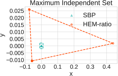
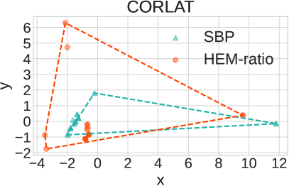
Figure 5: We perform principal component analysis on the cuts selected by HEM-ratio and SBP. Colored points illustrate the reduced cut features. The area covered by the dashed lines represents the diversity of selected cuts. The results show that HEM-ratio selects much more diverse cuts than SBP.

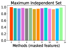
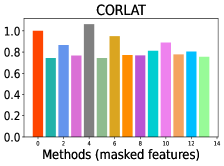
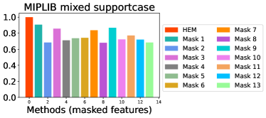
Figure 6: Evaluate the importance of the designed cut features. For the thirteen-dimensional features of a cut, we respectively set the $i$th dimension to zero, namely Mask $i$ ($i=1,2,\dots,13$). The results show the normalized performance of Mask $i$, defined by $\frac{M(\text{HEM})}{M(\text{Mask}\,\,i)}$. Here $M(\text{HEM})$ and $M(\text{Mask}\,\,i)$ denote the performance of HEM and Mask $i$, respectively.

TABLE X: Evaluation on Huawei production planning and order matching problems.

	Production planning ($n=3582.25,\,\,m=5040.42$)				Order matching ($n=67839.68,\,\,m=31364.84$)
Method	Time (s) $\downarrow$	Improvement $\uparrow$ (Time, %)	PD integral $\downarrow$	Improvement $\uparrow$ (PD integral, %)	Time (s) $\downarrow$	Improvement $\uparrow$ (Time, %)	PD integral $\downarrow$	Improvement$\uparrow$ (PD integral, %)
NoCuts	278.79 (231.02)	NA	17866.01 (21309.85)	NA	248.42 (287.29)	NA	403.41 (345.51)	NA
Default	296.12 (246.25)	-6.22	17703.39 (21330.40)	0.91	129.34 (224.24)	47.93	395.80 (341.23)	1.89
Random	280.18 (237.09)	-0.50	18120.21 (21660.01)	-1.42	95.76 (202.23)	61.45	406.73 (348.30)	-0.82
NV	259.48 (227.81)	6.93	17295.18 (21860.07)	3.20	245.61 (282.04)	1.13	406.69 (347.72)	-0.81
Eff	263.60 (229.24)	5.45	16636.52 (21322.89)	6.88	243.30 (276.65)	2.06	417.71 (360.13)	-3.54
SBP	276.61 (235.84)	0.78	16952.85 (21386.07)	5.11	44.14 (148.60)	82.23	379.23 (326.86)	5.99
HEM (Ours)	241.77 (229.97)	13.28	15751.08 (20683.53)	11.84	43.88 (148.66)	82.34	368.51 (309.02)	8.65

8.6 Visualization and explainability analysis

8.6.1 Diversity of selected cuts

We visualize the diversity of selected cuts, an important metric for evaluating whether the selected cuts complement each other nicely [18]. We visualize the cuts selected by HEM-ratio and SBP on a randomly sampled instance from Maximum Independent Set and CORLAT, respectively. We evaluate HEM-ratio rather than HEM, as HEM-ratio selects the same number of cuts as SBP. Furthermore, we perform principal component analysis on the selected cuts to reduce the cut features to two-dimensional space. Colored points illustrate the reduced cut features. To visualize the diversity of selected cuts, we use dashed lines to connect the points with the smallest and largest x,y coordinates. That is, the area covered by the dashed lines represents the diversity. Fig. 5 shows that SBP tends to select many similar cuts that are possibly redundant, especially on Maximum Independent Set. In contrast, HEM-ratio selects much more diverse cuts that can well complement each other. Please refer to Appendix E.2 for results on more datasets.

8.6.2 Analysis on structure of selected cuts

To provide further insight into learned policies by HEM, we analyze categories of the selected cuts by HEM on problems with knapsack constraints (specific structured problems). The results (see Appendix E.3) show that our learned model selects 92.03% and 99.5% cover inequalities (cover cuts) on Multiple Knapsack and MIK, respectively. It has been shown that a prominent category of cuts for knapsack problems is cover cuts [79, 80]. Therefore, the results suggest that our learned policies can well capture the underlying structure of specific structured problems, such as knapsack problems.

8.6.3 Feature analysis

To guide heuristics design for the cut selection, we conduct the following experiments to analyze the importance of features on the cut selection. Specifically, we evaluate the importance of each dimension feature by masking it. For the thirteen-dimensional features of a cut, we respectively set the $i$-th dimension to zero, namely Mask $i$ ($i=1,2,\dots,13$). Please refer to Appendix LABEL:appendix_cut_features for details of the thirteen-dimensional features. Fig 6 shows the normalized performance of Mask $i$ on Maximum Independent Set (MIS), CORLAT, and MIPLIB mixed supportcase. We define the normalized performance of Mask $i$ by $\frac{M(\text{HEM})}{M(\text{Mask}\,\,i)}$, where $M(\text{HEM})$ and $M(\text{Mask}\,\,i)$ denote the performance of HEM and Mask $i$, respectively. That is, the lower the normalized performance, the higher the corresponding Time and/or PD integral, indicating that the corresponding feature has more significant impact on cut selection. The results in Fig 6 suggest the following conclusions. First, most of the features have a significant impact on the performance, showing the effectiveness of our designed thirteen-dimensional features. Second, the 1st to 5th dimension features are widely used for heuristic design, while the results show that the 6th to 13th dimension features have a more significant impact on the cut selection. Therefore, incorporating the 6th to 13th dimension features into the heuristic design is important to improve the existing heuristics. Third, masking the 4th dimension feature improves the performance on CORLAT, suggesting that dropping the 4th dimension feature is beneficial when designing heuristics for the CORLAT dataset.

TABLE XI: Comparison between Default+ and Default. The best performance is marked in bold.

	Anonymous ($n=37881,\,\,m=49603$)			Production planning ($n=3582.25,\,\,m=5040.42$)			Order matching ($n=67839.68,\,\,m=31364.84$)
Method	Time (s) $\downarrow$	PD integral $\downarrow$	Improvement $\uparrow$ (%, PD integral)	Time (s) $\downarrow$	PD integral $\downarrow$	Improvement $\uparrow$ (%, PD integral)	Time (s) $\downarrow$	PD integral $\downarrow$	Improvement $\uparrow$ (%, PD integral)
NoCuts	246.22 (94.90)	18297.31 (9769.42)	NA	278.79 (231.02)	17866.01 (21309.86)	NA	248.42 (287.29)	403.41 (345.51)	NA
Default	244.02 (97.72)	17252.12 (9736.19)	5.71	296.12 (246.25)	17703.39 (21330.4)	0.91	129.34 (224.24)	395.80 (341.23)	1.89
Default+	242.59 (100.09)	16439.48 (9586.23)	10.15	280.40 (241.69)	17098.54 (21347.24)	4.30	129.04 (224.23)	380.27 (333.05)	5.74

8.7 Deployment in real-world challenging problems

8.7.1 Deploying learned policies

To further evaluate the effectiveness of our proposed HEM, we deploy HEM to large-scale real-world production planning and order matching problems at Huawei, which is one of the largest global commercial technology enterprises. Please refer to Appendix B.2 for details of the problems. The results in Table X show that HEM significantly outperforms all the baselines in terms of the Time and PD integral (up to 82.34% improvement). The results demonstrate the strong ability to enhance modern MILP solvers with HEM in real-world applications. Interestingly, Default performs poorer than NoCuts in production planning problems, which implies that an improper cut selection policy could significantly degrade the performance of MILP solvers.

8.7.2 Extracting order rules from our learned policies

To extract order rules from HEM as proposed in Section 7, we obtain the cutting plane categories with the highest number of times that is located at the first, second, and third position, respectively. We evaluate Default+ on three hard datasets as shown in Table XI. Please refer to Appendix E.10 for the statistical results and more evaluation results. The results show that Default+ outperforms Default in terms of the Time and PD integral (up to 4.44$\%$ improvement), which demonstrates the effectiveness of our extracted order rules. Therefore, Default+ is effective for simple and efficient deployment of our method into modern MILP solvers.

9 Conclusion

In this paper, we observe from extensive empirical results that the order of selected cuts has a significant impact on the efficiency of solving MILPs. We propose a novel hierarchical sequence/set model (HEM) to learn cut selection policies via reinforcement learning. Specifically, HEM is a two-level model: (1) a higher-level model to learn the number of cuts that should be selected, (2) and a lower-level model—that formulates the cut selection task as a sequence/set to sequence learning problem—to learn policies selecting an ordered subset with the cardinality determined by the higher-level model. Experiments show that HEM significantly improves the efficiency of solving MILPs compared to competitive baselines on both synthetic and large-scale real-world MILPs. We believe that our proposed approach brings new insights into learning cut selection.

Jie Wang received the B.Sc. degree in electronic information science and technology from University of Science and Technology of China, Hefei, China, in 2005, and the Ph.D. degree in computational science from the Florida State University, Tallahassee, FL, in 2011. He is currently a professor in the Department of Electronic Engineering and Information Science at University of Science and Technology of China, Hefei, China. His research interests include reinforcement learning, knowledge graph, large-scale optimization, deep learning, etc. He is a senior member of IEEE.

Zhihai Wang received the B.Sc. degree in Electrical and Electronic Engineering from Huazhong University of Science and Technology, Wuhan, China, in 2020. He is currently a Ph.D. candidate in the School of Data Science at University of Science and Technology of China, Hefei, China. His research interests include reinforcement learning and learning to optimize.

Xijun Li is a senior researcher of HUAWEI Noah’s Ark Lab. Before that, he has received M.Sc. degree from Shanghai Jiao Tong University, P.R. China, in 2018. He is working towards his Ph.D. degree in the University of Science and Technology of China (HUAWEI-USTC Joint Ph.D. Program) under the supervision of Prof. Jie Wang. He has published 10+ papers on top peer-reviewed conferences and journals (such as ICLR, KDD, ICDE, SIGMOD, DAC, CIKM, ICDCS, TCYB, etc.) and applied/published 12 patents (first author in 6 patents) with Noah’s Ark Lab. And he has won the championship of student learderboard in Dual Track of NeurIPS’21 ML4CO Competition. His recent research interests focus on Mathematical Programming Solver, Learning to Optimization (L2O) and Machine Learning for Computer System (ML4CS).

Yufei Kuang received the B.Sc. degree in Statistics from Nanjing University, Nanjing, China, in 2020. He is currently a Ph.D. candidate in Department of Electronic Engineering and Information Science at University of Science and Technology of China, Hefei, China. His research interests include reinforcement learning and learning to optimize.

Zhihao Shi received the B.Sc. degree in Department of Electronic Engineering and Information Science from University of Science and Technology of China, Hefei, China, in 2020. a Ph.D. candidate in the Department of Electronic Engineering and Information Science at University of Science and Technology of China, Hefei, China. His research interests include graph representation learning and natural language processing.

Fangzhou Zhu is currently a principal engineer in Noah’s Ark Lab, Huawei. He received the M.S degree from Soochow University. His current research interests include AI aided linear/mixed integer programming solver and its applications in supply chain management, especially for large scale industrial production planning problem. He is the key member of several supply chain optimization projects in Huawei.

Mingxuan Yuan is currently a principal researcher of Huawei Noah’s Ark Lab, Hong Kong. His research interests include data-driven optimization algorithms, data-driven SAT/MIP solving algorithms and data-driven EDA algorithm.

Jia Zeng received the B.Eng. degree from the Wuhan University of Technology, Wuhan, China, in 2002, and the Ph.D. degree from the City University of Hong Kong, Hong Kong, in 2007. He is currently the AI chief scientist for enterprise intelligence (e.g., supply chain management) at Huawei Noah’s Ark Lab, Hong Kong. He is also the director of the AI Strategic Planning and Cooperation Department. His research interests are foundation models, general problem solvers and embodied AI. He is a member of the CCF, the ACM and a senior member of the IEEE.

Yongdong Zhang received the Ph.D. degree in electronic engineering from Tianjin University, Tianjin, China, in 2002. He is currently a Professor at the University of Science and Technology of China. He has authored more than 100 refereed journal articles and conference papers. His current research interests include multimedia content analysis and understanding, multimedia content security, video encoding, and streaming media technology. He serves as an Editorial Board Member of Multimedia Systems journal and Neurocomputing. He was the recipient of the Best Paper Award in PCM 2013, ICIMCS 2013, and ICME 2010, and the Best Paper Candidate in ICME 2011. He is a Senior Member of IEEE.

Feng Wu received the B.S. degree in electrical engineering from Xidian University in 1992, and the M.S. and Ph.D. degrees in computer science from the Harbin Institute of Technology in 1996 and 1999, respectively. He is currently a Professor with the University of Science and Technology of China, where he is also the Dean of the School of Information Science and Technology. Before that, he was a Principal Researcher and the Research Manager with Microsoft Research Asia. His research interests include image and video compression, media communication, and media analysis and synthesis. He has authored or coauthored over 200 high quality articles (including several dozens of IEEE Transaction papers) and top conference papers on MOBICOM, SIGIR, CVPR, and ACM MM. He has 77 granted U.S. patents. His 15 techniques have been adopted into international video coding standards. As a coauthor, he received the Best Paper Award at 2009 IEEE Transactions on Circuits and Systems for Video Technology, PCM 2008, and SPIE VCIP 2007. He also received the Best Associate Editor Award from IEEE Circuits and Systems Society in 2012. He also serves as the TPC Chair for MMSP 2011, VCIP 2010, and PCM 2009, and the Special Sessions Chair for ICME 2010 and ISCAS 2013. He serves as an Associate Editor for IEEE Transactions on Circuits and Systems for Video Technology, IEEE Transactions ON Multimedia, and several other international journals.

Appendix A Proof

A.1 Proof of Proposition 1

Proof.

Please refer to Appendix A in our previous version in https://arxiv.org/abs/2302.00244. ∎

A.2 Proof of Proposition 2

Proof.

The optimization objective takes the form of

$$J(\theta)=\mathbb{E}_{s_{0},k_{0},a_{0}^{k}\dots}[\sum_{t=0}^{\infty}\gamma^{t}r(s_{t},k_{t},a_{t}^{k})],$$

where $s_{0}\sim\mu$, $(k_{t},a_{t}^{k})\sim\pi_{\theta}(\cdot|s_{t})$, $s_{t+1}=f(s_{t},a_{t})$, $\pi_{\theta}(k_{t},a_{t}^{k}|s_{t})=\pi^{h}_{\theta_{1}}(k_{t}|s_{t})\cdot\pi^{l}_{\theta_{2}}(a_{t}^{k}|s_{t},k_{t})$, and $\gamma\in(0,1]$ is the discount factor. Then we derive a hierarchical policy gradient under the multiple rounds setting as follows.

We first rewrite the objective as follows

$$J([\theta_{1},\theta_{2}]) =\mathbb{E}_{s_{0}\sim\mu}[V^{\pi_{\theta}}(s_{0})],$$

where $V^{\pi_{\theta}}(s_{0})$ denotes the state-value function.

We then compute the policy gradient for $\theta_{1}$:

$$\nabla_{\theta_{1}}J([\theta_{1},\theta_{2}])$$

$$=\mathbb{E}_{s_{0}\sim\mu}[\nabla_{\theta_{1}}\int_{(k_{0},a_{0}^{k_{0}})}\pi_{\theta}(k_{0},a_{0}^{k_{0}}|s_{0})Q^{\pi_{\theta}}(s_{0},k_{0},a_{0}^{k_{0}})d(k_{0},a_{0}^{k_{0}})]$$

$$=\mathbb{E}_{s_{0}\sim\mu}[\int_{(k_{0},a_{0}^{k_{0}})}\nabla_{\theta_{1}}\pi_{\theta}(k_{0},a_{0}^{k_{0}}|s_{0})Q^{\pi_{\theta}}(s_{0},k_{0},a_{0}^{k_{0}})d(k_{0},a_{0}^{k_{0}})]$$

$$+\mathbb{E}_{s_{0}\sim\mu}[\int_{(k_{0},a_{0}^{k_{0}})}\pi_{\theta}(k_{0},a_{0}^{k_{0}}|s_{0})\nabla_{\theta_{1}}Q^{\pi_{\theta}}(s_{0},k_{0},a_{0}^{k_{0}})d(k_{0},a_{0}^{k_{0}})]$$

$$=\mathbb{E}_{s_{0}\sim\mu,(k_{0},a_{0}^{k_{0}})\sim\pi_{\theta}}[\nabla_{\theta_{1}}\log(\pi_{\theta_{1}}^{h}(k_{0}|s_{0}))Q^{\pi_{\theta}}(s_{0},k_{0},a_{0}^{k_{0}})]$$

$$+\gamma\mathbb{E}_{s_{0}\sim\mu,(k_{0},a_{0}^{k_{0}})\sim\pi_{\theta},s_{1}=f}[\nabla_{\theta_{1}}V^{\pi_{\theta}}(s_{1})]$$

$$=\mathbb{E}_{s_{0}\sim\mu,(k_{0},a_{0}^{k_{0}})\sim\pi_{\theta}}[\nabla_{\theta_{1}}\log(\pi_{\theta_{1}}^{h}(k_{0}|s_{0}))Q^{\pi_{\theta}}(s_{0},k_{0},a_{0}^{k_{0}})$$

$$+\gamma\mathbb{E}_{s_{1}=f,(k_{1},a_{1}^{k_{1}})\sim\pi_{\theta}}[\nabla_{\theta_{1}}\log(\pi_{\theta_{1}}^{h}(k_{1}|s_{1}))Q^{\pi_{\theta}}(s_{1},k_{1},a_{1}^{k_{1}})]]$$

$$+\gamma^{2}\mathbb{E}_{s_{0}\sim\mu,(k_{0},a_{0}^{k_{0}})\sim\pi_{\theta},s_{1}=f,(k_{1},a_{1}^{k_{1}})\sim\pi_{\theta},s_{2}=f}[\nabla_{\theta_{1}}V^{\pi_{\theta}}(s_{2})]$$

$$=\cdots\cdots$$

$$=\mathbb{E}_{s\sim\rho^{\pi_{\theta}},(k,a^{k})\sim\pi_{\theta}}[Q^{\pi_{\theta}}(s,k,a^{k})\nabla_{\theta_{1}}\log(\pi_{\theta_{1}}^{h}(k|s))],$$

where $\rho^{\pi_{\theta}}(s)=\sum_{t=0}^{\infty}\gamma^{t}P(s_{t}=s|\pi_{\theta})$ denotes the expected state visitation frequencies under the policy $\pi_{\theta}$.

Similarly, we compute the policy gradient for $\theta_{2}$:

$$\nabla_{\theta_{2}}J([\theta_{1},\theta_{2}])$$

$$=\mathbb{E}_{s_{0}\sim\mu}[\nabla_{\theta_{2}}\int_{(k_{0},a_{0}^{k_{0}})}\pi_{\theta}(k_{0},a_{0}^{k_{0}}|s_{0})Q^{\pi_{\theta}}(s_{0},k_{0},a_{0}^{k_{0}})d(k_{0},a_{0}^{k_{0}})]$$

$$=\mathbb{E}_{s_{0}\sim\mu}[\int_{(k_{0},a_{0}^{k_{0}})}\nabla_{\theta_{2}}\pi_{\theta}(k_{0},a_{0}^{k_{0}}|s_{0})Q^{\pi_{\theta}}(s_{0},k_{0},a_{0}^{k_{0}})d(k_{0},a_{0}^{k_{0}})]$$

$$+\mathbb{E}_{s_{0}\sim\mu}[\int_{(k_{0},a_{0}^{k_{0}})}\pi_{\theta}(k_{0},a_{0}^{k_{0}}|s_{0})\nabla_{\theta_{2}}Q^{\pi_{\theta}}(s_{0},k_{0},a_{0}^{k_{0}})d(k_{0},a_{0}^{k_{0}})]$$

$$=\mathbb{E}_{s_{0}\sim\mu,(k_{0},a_{0}^{k_{0}})\sim\pi_{\theta}}[\nabla_{\theta_{2}}\log(\pi_{\theta_{2}}^{l}(a_{0}^{k_{0}}|s_{0},k_{0}))Q^{\pi_{\theta}}(s_{0},k_{0},a_{0}^{k_{0}})]$$

$$+\gamma\mathbb{E}_{s_{0}\sim\mu,(k_{0},a_{0}^{k_{0}})\sim\pi_{\theta},s_{1}=f}[\nabla_{\theta_{2}}V^{\pi_{\theta}}(s_{1})]$$

$$=\cdots\cdots$$

$$=\mathbb{E}_{s\sim\rho^{\pi_{\theta}},(k,a^{k})\sim\pi_{\theta}}[Q^{\pi_{\theta}}(s,k,a^{k})\nabla_{\theta_{2}}\log(\pi_{\theta_{2}}^{l}(a^{k}|s,k))],$$

where $\rho^{\pi_{\theta}}(s)=\sum_{t=0}^{\infty}\gamma^{t}P(s_{t}=s|\pi_{\theta})$ denotes the expected state visitation frequencies under the policy $\pi_{\theta}$.

We complete the proof.

∎

A.3 Proof of Proposition 3

In this part, we provide detailed proof of Proposition 3.

Proof.

Let $\mathbf{y}\in\mathbb{Z}\times(\left[0,d\right]\cap\mathbb{Z})^{n}$ satisfying $\mathbf{y}\leq_{L}\mathbf{z}$. The proposition is obvious if $\mathbf{y}=\mathbf{z}$ or for the index value $i=0$ (i.e., $y_{0}\leq\lfloor z_{0}\rfloor$).

So we assume now $\mathbf{y}\neq\mathbf{z}$ and $k\geq 0$ with $k=\text{argmin}_{j}\{y_{j}<z_{j}:j=0,\dots,n\}$. Notice that the definition of $k$ and the assumption $\mathbf{y}\leq_{L}\mathbf{z}$ imply $y_{q}=z_{q}$ for all $q\in\{0,\dots,k-1\}$. Thus the inequality (13) is trivially satisfied for all $i\in\{0,\dots,k\}$.

Now we consider the left hand-side of the inequality (13) for the case $i>k$. For the vector $\mathbf{y}$, we have

$$y_{i}+\sum_{j=0}^{i-1}a_{i-j}(y_{j}-\lceil z_{j}\rceil)$$

$$= y_{i}+\sum_{j=k}^{i-1}a_{i-j}(y_{j}-\lceil z_{j}\rceil)$$

$$\leq y_{i}-a_{i-k}+\sum_{j=k+1}^{i-1}a_{i-j}(y_{j}-\lceil z_{j}\rceil)\,\,(\text{as}\,\,y_{k}-\lceil z_{k}\rceil\leq-1)$$

$$\leq y_{i}-a_{i-k}+d\sum_{j=k+1}^{i-1}a_{i-j}\,\,(\text{as}\,\,y_{j}-\lceil z_{j}\rceil\leq d)$$

$$= y_{i}-a_{i-k}+d\sum_{j=1}^{i-k-1}a_{j}$$

$$= y_{i}-d\,\,(\text{as}\,\,a_{i-k}=d(1+\sum_{j=1}^{i-k-1}a_{j}))$$

$$\leq 0\leq\lfloor z_{i}\rfloor.$$

Now we complete the proof. ∎

A.4 Proof of Theorem 1

In this part, we provide detailed proof of Theorem 1, which follows [67]. To prove Theorem 1, we first introduce the following Lemmas.

Definition 2.

Given a vector $\mathbf{y}=(y_{0},\dots,y_{n})\in\mathbb{R}\times\left[0,d\right]^{n}$, $d\in\mathbb{Z}_{+}$, we define $\alpha(\mathbf{y})$ by the integral vector $\alpha(\mathbf{y})_{i}=\lfloor y_{i}\rfloor$ if $i\leq k$ and $\alpha(\mathbf{y})_{i}=d$ otherwise, for all $i\in\{0,\dots,n\}$, with $k=\text{argmin}_{j}\{y_{j}\not\in\mathbb{Z}:j=0,\dots,n\}$.

Lemma 1.

(Boundedness) Let $\mathbf{z}^{\star}=(z_{0},z_{1},\dots,z_{n})$ denote an optimal solution of the LP relaxation of the lexicographical optimization problem (11) (i.e., the problem (12)), and $\mathbf{x}^{\star}=(x_{0},x_{1},\dots,x_{n})$ denote an optimal integer solution of the lexicographical optimization problem (11). Then the following inequalities hold

$$(d\sum_{i=1}^{n}\min(0,c_{i}),0,\dots,0)\leq_{L}\mathbf{x}^{\star}\leq_{L}\alpha(\mathbf{z}^{\star})$$

Proof.

If $\mathbf{z}^{\star}$ is integral, the case is trivial. Thus, we focus on the case when $\mathbf{z}^{\star}$ is not integral. The left inequality stems from the bounds on the variables $x_{1},\dots,x_{n}$. The right inequality is due to the fact $\mathbf{z}^{\star}$ solves a relaxation of the problem solved by $\mathbf{x}^{\star}$, thus implying $\mathbf{x}^{\star}\leq_{L}\mathbf{z}^{\star}$, and since $\mathbf{x}^{\star}$ is integral we have $\mathbf{x}^{\star}\leq_{L}\alpha(\mathbf{z}^{\star})$. We complete the proof. ∎

Lemma 2.

(Monotonically Decreasing) Let $\mathbf{z}_{t}^{\star}$ denote an optimal solution of the linear programming relaxation problem that is solved at iteration $t$ in our focused cutting plane algorithm. Then, if $\mathbf{z}_{t}^{\star}$ and $\mathbf{z}_{t+1}^{\star}$ are not integral vectors, the following inequality holds: $\alpha(\mathbf{z}_{t+1}^{\star})<_{L}\alpha(\mathbf{z}_{t}^{\star})$

Proof.

Since the vectors $\mathbf{z}_{t}^{\star}$ and $\mathbf{z}_{t+1}^{\star}$ are not integral we have $\alpha(\mathbf{z}_{t}^{\star})<_{L}\mathbf{z}_{t}^{\star}$ and $\alpha(\mathbf{z}_{t+1}^{\star})<_{L}\mathbf{z}_{t+1}^{\star}$.

Next we aim to prove $\mathbf{z}_{t+1}^{\star}<_{L}\alpha(\mathbf{z}_{t}^{\star})$. To prove this, we first prove that the following inclusion holds

$$\mathbb{A}=\{\mathbf{x}\in\mathbb{Q}:\mathbf{x}\,\,\text{satisfies}\,\,(\ref{eq:cuts})_{k}\}\subseteq\mathbb{B}=\{\mathbf{x}\in\mathbb{Q}:\mathbf{x}\leq_{L}\alpha(\mathbf{z}_{t}^{\star})\},$$

where $\mathbb{Q}\subseteq\mathbb{R}\times\left[0,d\right]^{n}$, $\mathbb{Q}\subseteq\{\mathbf{x}\in\mathbb{R}^{n+1}:\mathbf{x}\leq_{L}\mathbf{z}_{t}^{\star}\}$, and $k=\text{argmin}_{i}\{z_{i}\not\in\mathbb{Z}:i=0,\dots,n\}$ ($\mathbf{z}_{t}^{\star}=(z_{0},\dots,z_{n})$).

To prove that, we show that for any vector $\mathbf{y}\in\mathbb{Q}\setminus\mathbb{B}$, then $\mathbf{y}\not\in\mathbb{A}$. Note that $\mathbf{y}\in\mathbb{Q}$ but $\alpha(\mathbf{z}_{t}^{\star})<_{L}\mathbf{y}$. As $\mathbb{Q}\subseteq\{\mathbf{x}\in\mathbb{R}^{n+1}:\mathbf{x}\leq_{L}\mathbf{z}_{t}^{\star}\}$ and $\mathbf{y}\in\mathbb{Q}$, we have $y_{i}=z_{i}$ for all $i\in\{0,1,\dots,k-1\}$. So the inequality $\alpha(\mathbf{z}_{t}^{\star})<_{L}\mathbf{y}$ implies $y_{k}>\lfloor z_{k}\rfloor$. Then $\mathbf{y}$ violates the inequality (13)_k as $y_{i}=z_{i}$ for all $i\in\{0,\dots,k-1\}$. That is, $\mathbf{y}\not\in\mathbb{A}$. Thus, we prove $\mathbb{A}\subseteq\mathbb{B}$.

Now we are ready to prove $\mathbf{z}_{t+1}^{\star}<_{L}\alpha(\mathbf{z}_{t}^{\star})$. As $\mathbf{z}_{t+1}^{\star}$ satisfies the inequality (13)_k, then $\mathbf{z}_{t+1}^{\star}\leq_{L}\alpha(\mathbf{z}_{t}^{\star})$. Due to the fact that $\mathbf{z}_{t+1}^{\star}$ is not integral, then $\mathbf{z}_{t+1}^{\star}<_{L}\alpha(\mathbf{z}_{t}^{\star})$. We complete the proof. ∎

Now we are ready to prove Theorem 1. We provide detailed proof as follows.

Proof.

Let $\mathbf{x}^{\star}$ denote an optimal integer solution of the lexmax problem (11). From Lemma 1, $\mathbf{x}^{\star}$ is bounded with $(d\sum_{i=1}^{n}\min(0,c_{i}),0,\dots,0)\leq_{L}\mathbf{x}^{\star}\leq_{L}\alpha(\mathbf{z}_{t}^{\star})$, where $\mathbf{z}_{t}^{\star}$ denotes an optimal solution of the LP relaxation problem solved at iteration $t$. Since the number of integer vectors that are lexicographically between $(d\sum_{i=1}^{n}\min(0,c_{i}),0,\dots,0)$ and $\alpha(\mathbf{z}_{t}^{\star})$ is finite, and from Lemma 2 we have $\alpha(\mathbf{z}_{t+1}^{\star})<_{L}\alpha(\mathbf{z}_{t}^{\star})$ whenever $\mathbf{z}_{t+1}^{\star}$ is not integral. Suppose $k=\text{argmin}_{i}\{\alpha(\mathbf{z}_{t+1}^{\star})_{i}<\alpha(\mathbf{z}_{t}^{\star})_{i}:i=0,\dots,n\}$, then $\alpha(\mathbf{z}_{t}^{\star})_{k}-\alpha(\mathbf{z}_{t+1}^{\star})_{k}\geq 1$. Thus, we get that an integer optimal solution is found in a finite number of iterations. From Lemma 1, the maximum number of iterations is $\mathcal{O}(d^{n+1}C)$ with $C=1+\sum_{i=1}^{n}|c_{i}|$. Now we complete the proof. ∎

Appendix B Details of the Datasets Used in this Paper

B.1 Datasets used in Section 4.1 in the main text

Please refer to Appendix D in our previous version in https://arxiv.org/abs/2302.00244.

B.2 Huawei’s large-scale real-world production planning and order matching problems

The production planning problem aims to find the optimal production planning for thousands of factories according to the daily order demand. The constraints include the production capacity for each production line in each factory, transportation limit, the order rate, etc. The optimization objective is to minimize the production cost and lead time simultaneously. We split the dataset into training and test sets with $80\%$ and $20\%$ of the instances. The average size of the production planning problems is approximately equal to $3500\times 5000=1.75\times 10^{8}$, which are large-scale real-world problems.

B.3 The datasets used in the main evaluation

Please refer to Appendix D in our previous version in https://arxiv.org/abs/2302.00244.

B.3.1 Detailed description of the aforementioned datasets

In this part, we provide detailed description of the aforementioned datasets. Note that all datasets we use except MIPLIB 2017 are application-specific, i.e., they contain instances from only a single application. We summarize the statistical description of the used datasets in this paper in Table LABEL:datasets. Let $n,m$ denote the average number of variables and constraints in the MILPs. Let $m\times n$ denote the size of the MILPs. We emphasize that the largest size of our used datasets is up to two orders of magnitude larger than that used in previous learning-based cut selection methods [19, 16], which demonstrates the superiority of our proposed HEM. Moreover, we test the inference time of our proposed HEM given the average number of candidate cuts. The results in Table LABEL:datasets show that the computational overhead of the HEM is very low.

Appendix C More Results

C.1 More results of comparative evaluation of HEM

Please refer to Appendix G in our previous version in https://arxiv.org/abs/2302.00244.

C.2 More results of comparative evaluation of HEM++

C.2.1 Evaluation under the multiple rounds setting

We compare HEM++ with the baselines under the multiple rounds setting on MIPLIB mixed neos as shown in Table XII. The results show that HEM++ significantly outperforms the baselines, improving the efficiency by up to 29.47%. This demonstrates that HEM++ is widely applicable to the multiple rounds setting.

C.2.2 Evaluation under the one round setting

We compare HEM++ with HEM under the one round setting on Maximum Independent Set, MIK, and CORLAT. The results in Table XIII show that HEM++ outperforms HEM on MIK (3.1% improvement in terms of the PD integral), and performs on par with HEM on Maximum Independent Set and CORLAT. This demonstrates the superiority of HEM++ over HEM.

TABLE XII: Evaluation of HEM++ under the multiple rounds setting on MIPLIB mixed neos.

	MIPLIB mixed neos
Method	Time (s)$\downarrow$	PD integral$\downarrow$	Improvement $\uparrow$ (PD integral, %)
NoCuts	253.65 (80.30)	14652.29 (12523.37)	NA
Default	258.31 (75.24)	12222.21 (12544.25)	16.58
Random	257.11 (74.61)	12606.61 (11884.03)	13.96
NV	254.63 (78.67)	13287.41 (11721.17)	9.32
Eff	263.78 (64.82)	11345.05 (12506.45)	22.57
SBP	258.90 (72.79)	11983.70 (12724.59)	18.21
HEM++ (Ours)	255.77 (77.37)	10334.00 (12537.6)	29.47

TABLE XIII: Evaluation of HEM++ under the one round setting.

	Maximum Independent Set			MIK			CORLAT
Method	Time (s) $\downarrow$	Improvement $\uparrow$ (%, Time)	PD integral$\downarrow$	Time (s)$\downarrow$	PD integral$\downarrow$	Improvement $\uparrow$ (%, PD integral)	Time (s)$\downarrow$	PD integral$\downarrow$	Improvement $\uparrow$ (%, PD integral)
NoCuts	8.78 (6.66)	NA	71.32 (51.74)	300.01 (0)	2355.87 (996.08)	NA	103.31 (128.14)	2818.41 (5908.31)	NA
Default	3.89 (5.04)	55.69	29.44 (35.28)	179.63 (122.36)	844.41 (924.30)	64.16	75.21 (120.30)	2412.09 (5892.88)	14.40
HEM (Ours)	1.76 (3.69)	80.00	16.01 (26.21)	176.12 (125.18)	785.05 (790.39)	66.68	58.31 (110.51)	1079.99 (2653.14)	61.68
HEM++ (Ours)	1.90 (4.22)	78.36	17.45 (30.83)	204.90 (111.52)	712.00 (777.09)	69.78	67.59 (119.51)	1091.53 (2214.94)	61.27

Appendix D Algorithm Implementation and Experimental Settings

D.1 Implementation details and hyperparameters

Please refer to Appendix F in our previous version in https://arxiv.org/abs/2302.00244.

D.2 Implementation details of HEM++

D.2.1 Details of the self-attention mechanism

Suppose there are $N$ candidate cuts, we denote each cut feature vector by $\textbf{c}_{i}$, $i=1,2,3,\dots,N$. We compute the query $\textbf{q}_{i}\in\mathbb{R}^{d_{k}}$, key $\textbf{k}_{i}\in\mathbb{R}^{d_{k}}$, and value $\textbf{v}_{i}\in\mathbb{R}^{d_{v}}$ for each cut by projecting the cut feature:

$$\textbf{q}_{i}=\textbf{W}^{Q}\textbf{c}_{i},\,\,\textbf{k}_{i}=\textbf{W}^{K}\textbf{c}_{i},\,\,\textbf{v}_{i}=\textbf{W}^{V}\textbf{c}_{i},$$

where $d_{k}$, $d_{v}$, and $d_{c}$ denote dimensions, $\textbf{W}^{Q}\in\mathbb{R}^{d_{k}\times d_{c}}$, $\textbf{W}^{K}\in\mathbb{R}^{d_{k}\times d_{c}}$, $\textbf{W}^{V}\in\mathbb{R}^{d_{v}\times d_{c}}$ are learnable parameters. Given the queries, keys, and values, we compute the embeddings by Scaled Dot-Product Attention [52]. Specifically, for the query $\textbf{q}_{i}$ of cut $i$ and the key $\textbf{k}_{i}$ of cut $j$, we compute the attention weight by

$$u_{ij}=\frac{\textbf{q}_{i}^{\top}\textbf{k}_{j}}{\sqrt{d_{k}}}.$$

We denote $\textbf{u}_{i}=\left[u_{i1},\dots u_{iN}\right]$. Finally, we compute the attention by

$$\textbf{c}_{i}^{\prime}=\sum_{j}\text{Softmax}(\textbf{u}_{i})_{j}\textbf{v}_{j},$$

where $\text{Softmax}(\textbf{u}_{i})_{j}$ denotes the $j$-th element of the softmax vector.

D.2.2 Details of the hierarchical proximal policy optimization method

Estimation of the advantage function We learn a state-value function $V_{\alpha}(s)$ as a baseline for reducing the variance of the advantage-function estimator. Following [47], we estimate the advantage-function by

$$\hat{A}(s,a)=G(s,a)-V_{\alpha}(s),$$

where $G(s,a)$ denotes the monte-carlo return [46].

Hyperparameters We apply the same optimizer and learning rates as that of HEM. For each epoch, we collect 32 samples, and we set the total epochs as 100. For each epoch, HEM performs one gradient update, while HEM++ performs ten gradient updates. Therefore, HEM++ is more sample-efficient than HEM. We set $\epsilon$ as 0.2.

D.3 More details of HEM

Please refer to Appendix F in our previous version in https://arxiv.org/abs/2302.00244.

D.4 Implementation details of the baselines

D.4.1 The one round setting

Please refer to Appendix F in our previous version in https://arxiv.org/abs/2302.00244.

D.4.2 The multiple rounds setting

For the human-designed baselines, they select a fixed ratio of cuts with high scores at each round until the cut separation procedure terminates. For SBP, it learns a scoring function to select a fixed ratio of cuts with high scores at each round until the cut separation procedure terminates, and achieves a return feedback for training the scoring function via evolutionary strategies.

Appendix E Additional Results

E.1 More results of ablation study

In this section, we provide more results of ablation studies in the main text.

E.1.1 In-depth analysis of HEM-ratio and SBP

We provide possible reasons for HEM-ratio performing poorer than SBP on several challenging MILP problem benchmarks. Fundamentally, HEM-ratio formulates the cut selection task as a sequence modeling problem, which has two main advantages over SBP. That is, the sequence model can not only capture the underlying order information, but also capture the interaction among cuts. However, training a sequence model is more difficult than training a scoring function, as the sequence model aims to learn a much more complex task. Specifically, the scoring function aims to learn to score each cut, while the sequence model aims to model the joint probability of the selected cuts. The latter is a more challenging learning task. Moreover, we follow the reinforcement learning paradigm instead of supervised learning to train the model, making the training process more unstable. Therefore, the sequence model may suffer from inefficient exploration and be trapped to a local optimum. As a result, HEM-ratio can perform poorer than SBP, especially on challenging MILP problem benchmarks.

E.1.2 Contribution of each component

Please refer to Appendix G in our previous version in https://arxiv.org/abs/2302.00244.

E.1.3 The importance of tackling P1-P3 in cut selection

Please refer to Appendix G in our previous version in https://arxiv.org/abs/2302.00244.

E.2 More visualization results

Please refer to Appendix G in our previous version in https://arxiv.org/abs/2302.00244.

E.3 Analysis on structure of selected cuts

We provide the results in Table XIV. Moreover, we analyze categories of the selected cuts by HEM++ on problems with knapsack constraints as well. The results in Table XIV show that policies learned by HEM++ select 90.95% and 99.6% cover inequalities (cover cuts) on Multiple Knapsack and MIK, respectively. Thus, the results suggest that HEM++ can also well capture the underlying structure of specific structured problems, such as knapsack problems.

TABLE XIV: HEM and HEM++ select more than 90% cover cuts, which is known as an important category of cuts for solving problems with knapsack constraints [79, 80].

Method	Knapsack problems	Percent of selected cover cuts (%)	Method	Knapsack problems	Percent of selected cover cuts (%)
HEM	Multiple Knapsack	92.03	HEM++	Multiple Knapsack	90.95
	MIK	99.5		MIK	99.6

E.4 Evaluation with a time limit of three hours

Please refer to Appendix G in our previous version in https://arxiv.org/abs/2302.00244.

E.5 Training curves

Please refer to Appendix G in our previous version in https://arxiv.org/abs/2302.00244.

E.6 Generalize to non-root nodes

In this part, we evaluate whether HEM can well generalize to non-root nodes. The results in Tables XV and XVI demonstrate that our learned models outperform the baselines for all nodes (both root and non-root nodes) under the one round setting and multiple rounds setting. Specifically, under the one round setting with non-root cuts, our model improves the Time and Primal-dual gap integral by up to 91.29% and 29.61%, respectively. Under the multiple rounds setting with non-root cuts, our model improves the Time and Primal-dual gap integral by up to 97.72% and 33.02%, respectively.

In a branch-and-bound search tree, modern solvers solve a linear programming (LP) relaxation of a Mixed-Integer Linear Program (MILP) at each node. Compared to adding cuts at root nodes, adding cuts at both root and non-root nodes would further strengthen the LP realaxations at non-root nodes, which thus may significantly improve the efficiency of solving MILPs. However, adding cuts at non-root nodes could lead to large models, which can increase the computational burden and present numerical instabilities [17, 16]. Therefore, whether to add cuts at non-root nodes relies on heuristics as well in real-world applications.

TABLE XV: The average performance of HEM and the baselines for non-root nodes under the one round setting. We obtain the results by deploying the models—which are learned at root nodes—to all nodes (root and non-root nodes). The best performance is marked in bold.

One round with non-root nodes	Easy: Maximum Independent Set			Hard: MIPLIB mixed supportcase
Method	Time (s)	Improvement (Time, %)	PD integral	Time (s)	PD integral	Improvement (PD integral, %)
NoCuts	8.78	NA	71.32	170.00	9927.96	NA
Default	1.47	83.25	13.95	128.89	9406.43	5.25
Random	2.07	76.47	20.78	124.65	9116.01	8.18
NV	3.21	63.42	29.81	134.58	8034.05	19.08
Eff	2.08	76.27	21.06	124.20	9035.90	8.99
HEM (Ours)	0.76	91.29	9.75	135.80	6987.87	29.61

TABLE XVI: The average performance of HEM++ and the baselines for non-root nodes under the multiple rounds setting. We obtain the results by deploying the models—which are learned at root nodes—to all nodes (root and non-root nodes).

Multiple rounds with non-root nodes	Easy: Maximum Independent Set			Hard: MIPLIB mixed supportcase
Method	Time (s)	Improvement (Time, %)	PD integral	Time (s)	PD integral	Improvement (PD integral, %)
NoCuts	8.78	NA	71.32	170.00	9927.96	NA
Default	0.28	96.78	6.41	123.13	8139.53	18.01
Random	1.04	88.11	11.00	125.03	9416.23	5.15
NV	1.14	87.05	12.05	107.78	7551.19	23.94
Eff	0.27	96.97	6.39	113.25	7246.07	27.01
HEM++ (Ours)	0.20	97.72	5.86	118.12	6649.86	33.02

TABLE XVII: Comparison between Default+ and Default on CORLAT.

	CORLAT
Method	Time (s) $\downarrow$	PD integral $\downarrow$	Improvement $\uparrow$(%, PD integral)
NoCuts	103.31 (128.14)	2818.41 (5908.31)	NA
Default	75.21 (120.30)	2412.09 (5892.88)	14.42
Default+	73.67 (119.14)	2315.50 (5765.29)	17.84

E.7 Generalize to other solvers

Our proposed methodology can well generalize to other solvers as shown in Table XVIII. The results demonstrate that HEM significantly outperforms the default cut selection method in the CBC solver [89] in terms of the primal-dual gap (up to 18.67% improvement).

We do not use commercial solvers, such as Gurobi [90] and [91], as the backend solver, since they do not provide interfaces for users to customize cut selection methods.

As the CBC cannot generate any cut on the dataset Maximum Independent Set, we conduct the experiments on the dataset Load balancing.

We use the primal-dual gap metric rather than the primal-dual gap integral due to the reasons as follows. (1) The primal-dual gap is a well-recognized metric for evaluating the solvers as well. (2) Unlike the SCIP, the CBC does not provide interfaces for users to acquire the primal-dual gap integral. Due to limited time, we do not implement the interface.

TABLE XVIII: The performance of HEM and the default strategy used in the CBC solver [89].

	MIPLIB mixed supportcase		Load balancing
Method	Primal dual gap (PD gap)	Improvement (%,PD gap)	Primal dual gap (PD gap)	Improvement (%,PD gap)
CBC Default	227.93	NA	0.98	NA
HEM (ours)	185.38	18.67	0.91	7.14

E.8 A detailed computational analysis of our model and the baselines’ model

We provide a detailed computational analysis of our proposed model and the baselines’ model in Table XIX. We summarize the conclusions in the following. (1) The training time of HEM and SBP is comparable, as most of their training time is spent on interacting with solvers to collect training samples. (2) The model parameters of HEM (212749) and SBP with LSTM (172289) are comparable. (3) The inference time of HEM is longer than that of SBP and SBP with LSTM. Nevertheless, the inference time of HEM (0.34s on average) is very low compared to the solving time (162s on average), especially on hard datasets. (4) The training of HEM is stable (please see Figure LABEL:fig:training_curves).

E.9 Measuring the primal and dual integrals

We have conducted experiments to measure the Primal Integral (PI) and Dual Integral (DI) as shown in Table XX. The results show that the performance improvement of HEM is from both the primal and dual sides.

Specifically, we use the optimal objective values as the reference values to measure the PI/DI. However, it is time-consuming to obtain optimal solutions for all instances. We conduct the experiments on three easy datasets due to limited time. Interestingly, the results demonstrate that proper cut selection policies can improve both the PI and DI. Moreover, the results show that HEM achieves more improvement from the primal side than the dual side on Set Cover and Maximum Independent Set, while HEM achieves more improvement from the dual side on Multiple Knapsack.

TABLE XIX: A detailed computational analysis of our model and the baselines’ model.

	Maximum Independent Set
	Model characteristics		Training			Testing
Model	Model paramters	GPU Memory (MB)	Training time (h)	Training samples	Avg Cuts	Inference time (s)	Performance/Time (s)
SBP	18433	2.07	3.03	3200	57	0.0003	2.43
SBP+LSTM encoder	172289	2.66	2.83			0.031	2.87
HEM (Ours)	212749	2.81	2.54			0.11	1.76

	MIPLIB mixed supportcase
	Model characteristics		Training			Testing
Model	Model paramters	GPU Memory	Training time (h)	Training samples	Avg Cuts	Inference time	Performance/PD integral
SBP	18433	2.07	13.81	3200	173	0.0004	7408.65
SBP+LSTM encoder	172289	2.66	13.24			0.033	7726.54
HEM (Ours)	212749	2.81	13.89			0.34	6874.8

TABLE XX: Evaluate the performance of HEM and Default in terms of the primal and dual integrals.

	Set Cover
Method	PrimalIntegral (PI)	Improvement (%, PI)	DualIntegral (DI)	Improvement (%, DI)
NoCuts	52.34	NA	59.85	NA
Default	45.02	13.99	49.95	16.54
HEM (ours)	28.84	44.90	35.95	39.93

	Maximum Independent Set
Method	PrimalIntegral (PI)	Improvement (%, PI)	DualIntegral (DI)	Improvement (%, DI)
NoCuts	66.83	NA	16.24	NA
Default	32.19	51.83	11.92	26.60
HEM (ours)	18.33	72.57	7.97	50.92

	Multiple Knapsack
Method	PrimalIntegral (PI)	Improvement (%, PI)	DualIntegral (DI)	Improvement (%, DI)
NoCuts	39.39	NA	41.62	NA
Default	25.40	35.52	25.70	38.25
HEM (ours)	19.24	51.16	18.90	54.59

E.10 More results of evaluation of Default+

We provide the statistical results on three hard datasets in Table XXII. Furthermore, we compare Defalut+ with Default on CORLAT as shown in Table XVII. The results show that Default+ outperforms Default (3.42% improvement in terms of the PD integral).

E.11 Industrial applicability of HEM

To thoroughly demonstrate that our proposed HEM is applicable to very large-scale datasets, we conduct the following experiments. Note that we use the SCIP [10], the state-of-the-art open-source solver, as our backend solver. First, we evaluate HEM on the entire MIPLIB dataset to demonstrate its applicability to very large-scale datasets. Second, we have deployed our HEM to a commercial solver, and further demonstrate its industrial applicability on security-constrained unit commitment (SCUC) problems from the electrical grid. Third, we analyze the model inference efficiency of HEM on large-scale datasets compared with simple scoring models to demonstrate that HEM is efficient on large-scale datasets as well.

Applicability of HEM to the Entire MIPLIB Dataset Given the entire MIPLIB dataset, we first follow Table LABEL:tab:Criteria to filter instances on which cut selection policies do not have a significant impact on the solving efficiency, which follows [15]. As a result, we evaluate HEM on a large MIPLIB dataset with 645 instances in total.

First, for validation and model selection, we randomly choose sixteen instances from the entire MIPLIB dataset as a validation set. The results in Table XXIII show that HEM outperforms the baselines in terms of the average solving time and primal-dual integral on the validation set, demonstrating the applicability of HEM to large-scale datasets. Second, we select the best model on the validation set, and compare the model with the Default cut selection strategy on all instances from the entire MIPLIB dataset. The results in Table XXIV (Left) show that HEM outperforms Default in terms of the average solving time and performs on par with Default in terms of the average primal-dual integral, further demonstrating the applicability of HEM to very large-scale datasets. Finally, we also report detailed performance of HEM and Default on each instance from the entire MIPLIB dataset in Tables XXV-XXXV. The results show that HEM struggles to consistently outperform Default on all instances from MIPLIB, as these instances are rather heterogeneous, posing significant challenges for machine learning methods [15]. Nevertheless, the results show that HEM can significantly outperform Default on many very large-scale instances, such as the instances neos-780889 (size $\approx 1.35\times 10^{10}$, 23.71% improvement, see Table XXXV) and map14860-20 (size $\approx 5.41\times 10^{10}$, 18.25% improvement, see Table XXXIII). The results further demonstrate the applicability of HEM to very large-scale datasets.

Industrial Applicability to a Commercial Solver In addition to the open source solver SCIP [10], we have deployed our HEM into a commercial solver (i.e., OptVerse [92] from Huawei) to further demonstrate the industrial applicability of HEM. (We do not use alternative commercial solvers, such as Gurobi [9] and Cplex [91], as they do not provide interfaces for users to customize cut selection methods based on their generated cuts. In contrast, the developers of OptVerse provide the interface for us to customize cut selection methods based on the generated cuts by OptVerse, which applies to the cut selection setting we focus on when using SCIP.) To demonstrate the strong ability of HEM to enhance commercial solvers, we compare HEM-OptVerse with Default-OptVerse on real SCUC problems from the electrical grid as shown in Table XXIV (Right). The results show that HEM-OptVerse significantly outperforms Default-OptVerse, improving the solving time by 8.99%.

Efficiency Analysis of HEM We provided a detailed computational analysis of HEM compared with simple scoring models in Appendix F.10. As shown in Table XIX, although the inference time of HEM (0.34 seconds on average) considerably exceeds that of scoring models (0.0004 seconds on average), the inference time for HEM remains rather low compared to the total solving time (162 seconds on average). Especially on large-scale datasets, the total solving time may significantly increase, whereas the model inference time of HEM exhibits only marginal changes. The major reason is that the model inference time of HEM is contingent on the number of input candidate cuts, while the number of candidate cuts remains consistent across varying dataset scales, typically ranging from 20 to 5,000. Therefore, the HEM model consistently maintains its inference efficiency when handling very large-scale datasets.

E.12 More Motivating Results

We present more motivating results on the order of selected cuts in Table XXI. The results show that adding the same selected cuts in different order significantly impacts the solver performance by up to orders of magnitude.

TABLE XXI: More motivating results on the order of selected cuts. The results show that adding the same selected cuts in different order significantly impacts the solver performance by up to orders of magnitude.

	Nodes
Instance name	Max	Min	Ratio
lectsched-5-obj	34993.00	2566.00	13.60
berlin	15534.00	1.00	15500.00

TABLE XXII: The cutting plane categories of selected cuts by our learned policies.

	Anonymous ($n=37881,\,\,m=49603$)		Production planning ($n=3582.25,\,\,m=5040.42$)		Order matching ($n=67839.68,\,\,m=31364.84$)
Ranking	Category	Percent (%)	Category	Percent (%)	Category	Percent (%)
The first	Implbd	50	Implbd	60	Intobj	90
The second	Knapsack Cover	45	Gomory	50	Implbd	30
The third	Gomory	35	Clique	50	Knapsack cover	50

TABLE XXIII: Evaluation of HEM on the validation set of the entire MIPLIB dataset.

	MIPLIB Entire Validation Set
Method	Time (s)	Improvement (%, Time)	PD integral	Improvement (%, PD integral)
NoCuts	265.31 (86.24)	NA	11566.19 (12644.29)	NA
Default	253.79 (97.92)	4.34	10809.30 (12217.92)	6.54
Random	263.64 (85.60)	0.63	11174.70 (12462)	3.38
NV	263.10 (89.31)	0.83	11260.19 (12482.14)	2.65
Eff	263.03 (88.06)	0.86	11143.30 (12479.65)	3.66
HEM (Ours)	249.16 (105.36)	6.09	10172.41 (12251.67)	12.05

TABLE XXIV: (Left) Evaluation of HEM on all instances from the entire MIPLIB dataset. (Right) Evaluation of HEM in the OptVerse commercial solver on the SCUC problems.

	MIPLIB Entire All Instances				SCUC Problems
Method	Time (s)	Improvement (%, Time)	PD integral	Improvement (%, PD integral)	Method	Time (s)	Improvement (%, Time)
Default	242.14 (109.21)	NA	13331.06 (11877.49)	NA	Default-OptVerse	76.01	NA
HEM (Ours)	237.00 (113.11)	2.12	13425.27 (11781.09)	-0.71	HEM-OptVerse (Ours)	69.18	8.99

TABLE XXV: Evaluation of HEM on all instances from the MIPLIB dataset. In particular, HEM improves the solving time by two orders of magnitude compared to Default on the berlin benchmark.

Instance name	Method	Time (s)	PD integral	Instance name	Method	Time (s)	PD integral
supportcase7	HEM (Ours)	171.03	10293.18	istanbul-no-cutoff	HEM (Ours)	268.96	10945.90
supportcase7	Default	161.56	5079.67	istanbul-no-cutoff	Default	233.91	8885.47
neos-4413714-turia	HEM (Ours)	303.26	30325.68	dws012-03	HEM (Ours)	300.03	30002.59
neos-4413714-turia	Default	300.11	30011.48	dws012-03	Default	300.01	30001.06
loopha13	HEM (Ours)	300.00	30000.04	neos-826650	HEM (Ours)	300.00	30000.05
loopha13	Default	300.01	30000.64	neos-826650	Default	300.00	30000.08
bppc6-06	HEM (Ours)	300.01	3594.09	neos-848589	HEM (Ours)	321.08	32107.58
bppc6-06	Default	300.00	3620.68	neos-848589	Default	314.24	31423.79
dc1c	HEM (Ours)	300.00	29159.48	beasleyC3	HEM (Ours)	300.00	15360.70
dc1c	Default	300.01	29226.89	beasleyC3	Default	300.00	12069.52
pk1	HEM (Ours)	124.40	6624.47	neos-2746589-doon	HEM (Ours)	303.17	30317.19
pk1	Default	117.49	5230.99	neos-2746589-doon	Default	302.09	30209.27
pigeon-10	HEM (Ours)	11.29	121.98	opm2-z6-s1	HEM (Ours)	209.48	2893.50
pigeon-10	Default	48.81	495.60	opm2-z6-s1	Default	112.28	3270.46
cvs08r139-94	HEM (Ours)	300.00	5206.78	neos-1122047	HEM (Ours)	3.11	305.67
cvs08r139-94	Default	300.00	5151.11	neos-1122047	Default	2.58	253.50
nursesched-medium-hint03	HEM (Ours)	301.49	30148.71	sct31	HEM (Ours)	300.00	16833.62
nursesched-medium-hint03	Default	301.33	30132.67	sct31	Default	300.00	13478.60
rail507	HEM (Ours)	86.80	2989.06	p200x1188c	HEM (Ours)	300.00	1905.48
rail507	Default	300.00	3944.25	p200x1188c	Default	300.00	12400.04
supportcase16	HEM (Ours)	0.08	1.74	set3-16	HEM (Ours)	300.00	27850.42
supportcase16	Default	0.04	1.39	set3-16	Default	300.01	27016.62
supportcase23	HEM (Ours)	300.03	30002.70	berlin-5-8-0	HEM (Ours)	300.01	6731.06
supportcase23	Default	300.01	30001.06	berlin-5-8-0	Default	300.02	9014.56
acc-tight5	HEM (Ours)	84.49	8448.84	lectsched-5-obj	HEM (Ours)	300.00	30000.07
acc-tight5	Default	101.05	10104.33	lectsched-5-obj	Default	300.02	23713.00
allcolor58	HEM (Ours)	300.91	30080.31	neos-860300	HEM (Ours)	27.67	1338.58
allcolor58	Default	301.69	30137.51	neos-860300	Default	38.63	1668.05
ger50-17-trans-dfn-3t	HEM (Ours)	300.01	10570.45	s1234	HEM (Ours)	300.00	26716.95
ger50-17-trans-dfn-3t	Default	300.00	10640.70	s1234	Default	300.00	29946.33
neos8	HEM (Ours)	0.78	50.96	berlin	HEM (Ours)	1.80	168.78
neos8	Default	0.56	45.08	berlin	Default	300.00	22556.29
tokyometro	HEM (Ours)	300.01	25223.99	neos-3555904-turama	HEM (Ours)	302.25	30225.28
tokyometro	Default	300.00	27916.23	neos-3555904-turama	Default	301.04	30103.83
gsvm2rl5	HEM (Ours)	300.00	20977.88	dano3mip	HEM (Ours)	300.04	9827.41
gsvm2rl5	Default	300.00	20963.11	dano3mip	Default	300.05	9912.95
pigeon-20	HEM (Ours)	300.00	1787.69	aligninq	HEM (Ours)	0.37	37.32
pigeon-20	Default	300.00	1677.25	aligninq	Default	9.40	91.95
supportcase41	HEM (Ours)	300.33	30032.56	dsbmip	HEM (Ours)	0.68	36.07
supportcase41	Default	300.51	30051.07	dsbmip	Default	0.95	36.81
neos-3209519-ruhr	HEM (Ours)	300.00	13249.40	snp-02-004-104	HEM (Ours)	300.02	30001.73
neos-3209519-ruhr	Default	300.00	13894.18	snp-02-004-104	Default	300.03	30002.84
neos-5195221-niemur	HEM (Ours)	300.00	30000.40	n13-3	HEM (Ours)	41.41	201.20
neos-5195221-niemur	Default	300.00	30000.32	n13-3	Default	18.66	86.40
pw-myciel4	HEM (Ours)	300.00	17285.62	probportfolio	HEM (Ours)	300.00	14867.88
pw-myciel4	Default	300.00	16387.31	probportfolio	Default	300.00	17571.52
beavma	HEM (Ours)	3.41	23.93	neos-1337307	HEM (Ours)	300.00	30000.09
beavma	Default	1.51	9.06	neos-1337307	Default	300.00	30000.01

TABLE XXVI: Evaluation of HEM on all instances from the MIPLIB dataset.

Instance name	Method	Time (s)	PD integral	Instance name	Method	Time (s)	PD integral
neos-3759587-noosa	HEM (Ours)	31.99	3198.11	nexp-150-20-8-5	HEM (Ours)	109.70	10445.19
neos-3759587-noosa	Default	24.19	2418.13	nexp-150-20-8-5	Default	300.00	24821.33
neos-4343293-stony	HEM (Ours)	300.00	18256.30	ns1849932	HEM (Ours)	300.09	30008.95
neos-4343293-stony	Default	300.00	18456.28	ns1849932	Default	303.24	30323.93
radiationm40-10-02	HEM (Ours)	300.00	12987.75	beasleyC1	HEM (Ours)	10.34	167.80
radiationm40-10-02	Default	300.01	13722.23	beasleyC1	Default	9.36	150.95
ns4-pr6	HEM (Ours)	176.37	38.35	supportcase40	HEM (Ours)	300.00	2730.05
ns4-pr6	Default	95.15	27.33	supportcase40	Default	300.00	2647.49
neos-3594536-henty	HEM (Ours)	300.07	2420.84	p500x2988c	HEM (Ours)	1.80	34.49
neos-3594536-henty	Default	300.02	2382.38	p500x2988c	Default	1.70	27.24
rmatr100-p5	HEM (Ours)	300.00	5882.44	neos-826224	HEM (Ours)	90.66	2382.46
rmatr100-p5	Default	300.00	5358.22	neos-826224	Default	68.73	1264.98
neos-5076235-embley	HEM (Ours)	300.00	8175.26	h80x6320d	HEM (Ours)	300.01	5108.96
neos-5076235-embley	Default	300.01	7750.12	h80x6320d	Default	300.00	4944.07
trento1	HEM (Ours)	300.00	23876.76	opm2-z8-s0	HEM (Ours)	300.01	13770.78
trento1	Default	300.00	23849.69	opm2-z8-s0	Default	300.01	14525.46
neos-1420546	HEM (Ours)	300.00	5037.73	neos-4650160-yukon	HEM (Ours)	300.01	30000.06
neos-1420546	Default	300.02	4850.51	neos-4650160-yukon	Default	300.01	30000.32
n3700	HEM (Ours)	300.00	7498.37	sp97ic	HEM (Ours)	300.00	5709.25
n3700	Default	300.00	7435.09	sp97ic	Default	300.00	5037.69
gen	HEM (Ours)	0.11	1.44	lectsched-4-obj	HEM (Ours)	25.60	1696.96
gen	Default	0.08	1.38	lectsched-4-obj	Default	11.25	784.84
neos-885086	HEM (Ours)	300.00	1253.43	opm2-z7-s8	HEM (Ours)	300.00	6143.38
neos-885086	Default	300.00	1170.84	opm2-z7-s8	Default	300.00	8607.81
misc07	HEM (Ours)	14.55	447.29	traininstance2	HEM (Ours)	300.00	30000.03
misc07	Default	13.70	335.85	traininstance2	Default	300.00	30000.09
mushroom-best	HEM (Ours)	300.01	30000.96	nexp-150-20-1-5	HEM (Ours)	200.70	2813.87
mushroom-best	Default	300.01	29928.88	nexp-150-20-1-5	Default	300.00	3932.13
neos-831188	HEM (Ours)	300.00	8511.26	supportcase33	HEM (Ours)	300.00	15960.48
neos-831188	Default	271.02	13374.50	supportcase33	Default	300.00	10689.37
comp21-2idx	HEM (Ours)	300.01	29916.77	biella1	HEM (Ours)	300.01	17763.66
comp21-2idx	Default	300.00	29933.48	biella1	Default	300.00	16829.23
triptim1	HEM (Ours)	301.28	27250.01	neos-5107597-kakapo	HEM (Ours)	300.00	26195.32
triptim1	Default	301.22	24026.33	neos-5107597-kakapo	Default	300.00	23588.92
neos-4722843-widden	HEM (Ours)	300.03	29153.77	rmatr200-p5	HEM (Ours)	301.83	15330.00
neos-4722843-widden	Default	300.01	28724.77	rmatr200-p5	Default	303.42	15337.71
k16x240b	HEM (Ours)	300.01	8520.64	ds	HEM (Ours)	302.74	29271.58
k16x240b	Default	300.01	10078.17	ds	Default	442.52	42586.65
noswot	HEM (Ours)	33.90	159.88	rd-rplusc-21	HEM (Ours)	300.00	29995.52
noswot	Default	29.00	137.19	rd-rplusc-21	Default	300.00	29994.70
sct2	HEM (Ours)	300.00	452.80	50v-10	HEM (Ours)	300.00	2188.96
sct2	Default	300.00	401.39	50v-10	Default	300.00	2235.31
app1-1	HEM (Ours)	0.63	58.12	piperout-d27	HEM (Ours)	30.88	2454.01
app1-1	Default	0.57	53.14	piperout-d27	Default	26.46	2038.97
nu120-pr12	HEM (Ours)	7.42	73.98	rococoB10-011000	HEM (Ours)	116.21	5075.11
nu120-pr12	Default	7.99	77.28	rococoB10-011000	Default	300.00	12744.09
ns1904248	HEM (Ours)	300.05	30005.07	ci-s4	HEM (Ours)	44.41	2484.01
ns1904248	Default	300.03	30003.47	ci-s4	Default	29.99	1456.73
khb05250	HEM (Ours)	0.90	8.02	gen-ip036	HEM (Ours)	300.00	96.82
khb05250	Default	0.48	5.82	gen-ip036	Default	300.00	76.63
eva1aprime6x6opt	HEM (Ours)	300.00	30000.10	neos-957323	HEM (Ours)	300.00	7465.30
eva1aprime6x6opt	Default	300.00	30000.07	neos-957323	Default	261.26	4902.44

TABLE XXVII: Evaluation of HEM on all instances from the MIPLIB dataset.

Instance name	Method	Time (s)	PD integral	Instance name	Method	Time (s)	PD integral
neos-3656078-kumeu	HEM (Ours)	300.67	30067.06	g200x740	HEM (Ours)	300.00	4194.39
neos-3656078-kumeu	Default	300.12	30012.27	g200x740	Default	300.00	2361.11
neos-954925	HEM (Ours)	302.97	8384.86	neos-3426085-ticino	HEM (Ours)	49.43	278.56
neos-954925	Default	302.01	7483.41	neos-3426085-ticino	Default	300.03	2467.60
ran13x13	HEM (Ours)	70.75	425.67	pigeon-08	HEM (Ours)	4.90	68.65
ran13x13	Default	70.71	427.02	pigeon-08	Default	2.32	34.96
bab6	HEM (Ours)	305.49	30549.37	dfn-bwin-DBE	HEM (Ours)	300.00	23767.69
bab6	Default	302.72	30272.30	dfn-bwin-DBE	Default	300.00	15899.51
toll-like	HEM (Ours)	300.01	24007.09	reblock115	HEM (Ours)	300.00	1092.33
toll-like	Default	300.00	22759.58	reblock115	Default	300.00	1188.85
neos16	HEM (Ours)	300.00	1685.31	swath	HEM (Ours)	300.02	24022.99
neos16	Default	300.00	3240.90	swath	Default	300.02	24629.17
prod1	HEM (Ours)	27.64	81.42	gmut-76-50	HEM (Ours)	301.42	3754.92
prod1	Default	17.56	38.25	gmut-76-50	Default	300.47	3756.05
core4284-1064	HEM (Ours)	130.64	10829.49	23588	HEM (Ours)	3.44	92.92
core4284-1064	Default	300.05	11455.30	23588	Default	3.75	74.57
qnet1-o	HEM (Ours)	2.25	53.94	sorrell8	HEM (Ours)	300.00	23264.84
qnet1-o	Default	1.08	28.37	sorrell8	Default	300.00	22577.85
neos-3530905-gaula	HEM (Ours)	300.01	2563.14	neos-5221106-oparau	HEM (Ours)	300.14	30014.36
neos-3530905-gaula	Default	300.00	3239.95	neos-5221106-oparau	Default	300.01	30001.32
rocII-8-11	HEM (Ours)	300.01	30001.22	timtab1	HEM (Ours)	300.00	4917.39
rocII-8-11	Default	300.00	28339.99	timtab1	Default	300.00	4592.97
drayage-25-23	HEM (Ours)	300.00	2197.62	neos-1599274	HEM (Ours)	106.18	391.20
drayage-25-23	Default	300.00	1337.71	neos-1599274	Default	2.97	205.71
neos-4300652-rahue	HEM (Ours)	300.94	20093.16	neos-3755335-nizao	HEM (Ours)	160.09	16005.79
neos-4300652-rahue	Default	300.36	30036.35	neos-3755335-nizao	Default	221.12	22094.23
neos-3634244-kauru	HEM (Ours)	340.74	33930.05	fiber	HEM (Ours)	2.88	110.70
neos-3634244-kauru	Default	317.65	31627.44	fiber	Default	1.97	66.96
pigeon-13	HEM (Ours)	300.00	2367.16	bppc8-09	HEM (Ours)	300.00	1406.41
pigeon-13	Default	300.00	2491.82	bppc8-09	Default	300.00	1501.39
neos17	HEM (Ours)	20.16	972.65	decomp1	HEM (Ours)	96.83	1717.15
neos17	Default	31.42	1065.50	decomp1	Default	84.68	1363.22
ex1010-pi	HEM (Ours)	41.94	1862.29	scpj4scip	HEM (Ours)	302.75	15882.32
ex1010-pi	Default	300.01	6584.58	scpj4scip	Default	302.12	15494.02
aflow30a	HEM (Ours)	17.06	153.51	queens-30	HEM (Ours)	300.83	16375.54
aflow30a	Default	36.70	279.27	queens-30	Default	300.81	16749.56
mzzv42z	HEM (Ours)	300.00	9108.06	mas76	HEM (Ours)	57.65	60.67
mzzv42z	Default	300.00	10904.81	mas76	Default	82.96	98.18
glass-sc	HEM (Ours)	300.00	8062.51	b2c1s1	HEM (Ours)	300.00	20027.00
glass-sc	Default	300.00	8806.45	b2c1s1	Default	300.00	21464.96
neos-820879	HEM (Ours)	122.10	829.58	flugpl	HEM (Ours)	0.03	1.92
neos-820879	Default	121.04	681.68	flugpl	Default	0.03	1.62
sct5	HEM (Ours)	300.01	26036.69	piperout-27	HEM (Ours)	38.67	3792.68
sct5	Default	300.01	21415.71	piperout-27	Default	50.71	2633.38
neos-3610173-itata	HEM (Ours)	1.29	7.87	cost266-UUE	HEM (Ours)	300.00	3577.97
neos-3610173-itata	Default	6.67	23.33	cost266-UUE	Default	300.00	3291.35
fhnw-schedule-paira100	HEM (Ours)	300.00	24805.57	chromaticindex512-7	HEM (Ours)	302.00	15707.05
fhnw-schedule-paira100	Default	300.00	25636.38	chromaticindex512-7	Default	301.17	15050.59
fhnw-schedule-paira400	HEM (Ours)	300.02	29928.81	tbfp-bigm	HEM (Ours)	300.00	29952.53
fhnw-schedule-paira400	Default	301.10	30026.32	tbfp-bigm	Default	300.00	29960.21

TABLE XXVIII: Evaluation of HEM on all instances from the MIPLIB dataset.

Instance name	Method	Time (s)	PD integral	Instance name	Method	Time (s)	PD integral
neos-933638	HEM (Ours)	300.00	24675.26	cmflsp50-24-8-8	HEM (Ours)	300.00	30000.35
neos-933638	Default	300.00	25978.22	cmflsp50-24-8-8	Default	300.00	30000.48
supportcase18	HEM (Ours)	300.01	1230.69	piperout-03	HEM (Ours)	37.54	1390.49
supportcase18	Default	300.00	2327.46	piperout-03	Default	20.24	627.14
f2000	HEM (Ours)	300.02	30001.84	qnet1	HEM (Ours)	1.84	45.97
f2000	Default	300.02	30002.42	qnet1	Default	2.00	47.09
neos-686190	HEM (Ours)	88.88	2485.56	rmatr200-p10	HEM (Ours)	300.22	16754.09
neos-686190	Default	155.26	3565.51	rmatr200-p10	Default	300.19	15937.30
neos-933562	HEM (Ours)	300.00	30000.01	chromaticindex32-8	HEM (Ours)	4.03	138.76
neos-933562	Default	300.00	30000.04	chromaticindex32-8	Default	3.35	116.37
mkc	HEM (Ours)	300.00	3131.59	map18	HEM (Ours)	300.00	5204.01
mkc	Default	300.00	3346.59	map18	Default	300.00	5011.93
iis-glass-cov	HEM (Ours)	300.00	7225.48	neos-3682128-sandon	HEM (Ours)	300.00	19986.91
iis-glass-cov	Default	300.00	6901.28	neos-3682128-sandon	Default	300.00	20126.59
neos9	HEM (Ours)	302.83	30283.37	mas74	HEM (Ours)	300.01	2090.64
neos9	Default	301.44	30143.57	mas74	Default	300.01	1772.69
neos-3072252-nete	HEM (Ours)	300.00	2818.27	cmflsp40-24-10-7	HEM (Ours)	300.00	30000.15
neos-3072252-nete	Default	300.00	2648.87	cmflsp40-24-10-7	Default	300.00	30000.15
nursesched-sprint-hidden09	HEM (Ours)	300.00	23875.48	sing44	HEM (Ours)	302.94	21962.78
nursesched-sprint-hidden09	Default	300.00	26334.48	sing44	Default	339.78	19856.41
CMS750-4	HEM (Ours)	300.11	10259.69	d20200	HEM (Ours)	80.33	663.53
CMS750-4	Default	300.09	17546.64	d20200	Default	300.00	890.47
neos-872648	HEM (Ours)	301.79	30082.42	n3seq24	HEM (Ours)	305.31	25521.89
neos-872648	Default	302.60	30037.89	n3seq24	Default	303.75	25054.17
neos-2328163-agri	HEM (Ours)	300.00	23106.49	blend2	HEM (Ours)	2.15	114.03
neos-2328163-agri	Default	300.00	21578.56	blend2	Default	1.74	86.10
neos-4647032-veleka	HEM (Ours)	300.92	12766.14	sorrell4	HEM (Ours)	325.99	32165.08
neos-4647032-veleka	Default	300.70	11494.80	sorrell4	Default	300.16	29585.77
swath2	HEM (Ours)	78.73	1299.74	graphdraw-domain	HEM (Ours)	300.00	9788.69
swath2	Default	62.34	914.19	graphdraw-domain	Default	300.00	8768.64
dws012-02	HEM (Ours)	300.01	30000.67	ns930473	HEM (Ours)	300.00	30000.26
dws012-02	Default	300.00	30000.15	ns930473	Default	300.00	30000.40
xmas10-2	HEM (Ours)	300.00	30000.12	neos-2657525-crna	HEM (Ours)	300.00	30000.01
xmas10-2	Default	300.00	30000.09	neos-2657525-crna	Default	300.00	30000.03
map10	HEM (Ours)	300.17	14424.14	neos-5100895-inster	HEM (Ours)	300.00	10350.73
map10	Default	300.07	12881.00	neos-5100895-inster	Default	300.01	8617.35
neos-480878	HEM (Ours)	18.29	71.25	neos-5106984-jizera	HEM (Ours)	300.21	30021.09
neos-480878	Default	15.10	63.28	neos-5106984-jizera	Default	300.22	30022.01
gsvm2rl3	HEM (Ours)	300.01	11329.37	air05	HEM (Ours)	56.32	1009.90
gsvm2rl3	Default	300.01	10835.78	air05	Default	71.97	936.17
graph20-20-1rand	HEM (Ours)	300.00	22132.47	neos-1223462	HEM (Ours)	34.32	3432.17
graph20-20-1rand	Default	300.00	23225.13	neos-1223462	Default	39.40	3940.09
supportcase37	HEM (Ours)	215.15	16566.21	ns1208400	HEM (Ours)	300.00	30000.41
supportcase37	Default	176.08	12669.59	ns1208400	Default	300.00	30000.15
icir97-potential	HEM (Ours)	300.00	2446.99	adult-max5features	HEM (Ours)	304.02	30401.69
icir97-potential	Default	300.00	2092.13	adult-max5features	Default	302.64	30263.81
supportcase34	HEM (Ours)	300.01	23074.16	n370b	HEM (Ours)	300.00	7381.95
supportcase34	Default	300.01	16989.15	n370b	Default	300.00	7302.67
neos-824661	HEM (Ours)	300.00	12156.04	cap6000	HEM (Ours)	19.17	31.50
neos-824661	Default	282.44	8809.19	cap6000	Default	6.35	26.30
neos-3046601-motu	HEM (Ours)	300.01	21564.43	10teams	HEM (Ours)	80.39	2008.06
neos-3046601-motu	Default	300.01	20851.82	10teams	Default	59.54	1047.81

TABLE XXIX: Evaluation of HEM on all instances from the MIPLIB dataset.

Instance name	Method	Time (s)	PD integral	Instance name	Method	Time (s)	PD integral
manna81	HEM (Ours)	300.01	155.57	adult-regularized	HEM (Ours)	303.61	30360.54
manna81	Default	0.88	24.43	adult-regularized	Default	303.07	30307.08
n6-3	HEM (Ours)	300.02	7110.18	neos-4355351-swalm	HEM (Ours)	306.36	30636.41
n6-3	Default	300.00	6411.26	neos-4355351-swalm	Default	305.05	30504.98
markshare2	HEM (Ours)	300.02	30000.00	neos-3216931-puriri	HEM (Ours)	300.00	30000.12
markshare2	Default	300.02	30000.00	neos-3216931-puriri	Default	300.00	30000.09
dcmulti	HEM (Ours)	0.69	4.48	app3	HEM (Ours)	1.53	39.94
dcmulti	Default	0.69	4.42	app3	Default	1.79	25.03
neos-4805882-barwon	HEM (Ours)	300.00	6050.70	roi2alpha3n4	HEM (Ours)	300.00	14683.88
neos-4805882-barwon	Default	300.00	5301.15	roi2alpha3n4	Default	300.05	14408.90
neos-555343	HEM (Ours)	300.00	4260.10	neos-911970	HEM (Ours)	300.00	9253.47
neos-555343	Default	300.00	4281.19	neos-911970	Default	300.00	8283.90
academictimetablesmall	HEM (Ours)	300.00	30000.30	lr1dr02vc05v8a-t360	HEM (Ours)	300.01	28018.01
academictimetablesmall	Default	300.01	30000.62	lr1dr02vc05v8a-t360	Default	300.00	28922.64
neos-4306827-ravan	HEM (Ours)	302.44	30244.39	neos-662469	HEM (Ours)	300.01	17974.07
neos-4306827-ravan	Default	301.92	30191.67	neos-662469	Default	300.00	21617.42
neos-885524	HEM (Ours)	300.06	3971.59	nsa	HEM (Ours)	0.60	3.47
neos-885524	Default	234.66	3611.65	nsa	Default	0.58	3.52
supportcase39	HEM (Ours)	300.06	30006.26	neos-1067731	HEM (Ours)	300.00	13095.86
supportcase39	Default	300.00	30000.24	neos-1067731	Default	300.00	12973.48
blp-ar98	HEM (Ours)	300.05	11818.11	ns1111636	HEM (Ours)	305.43	28696.39
blp-ar98	Default	300.00	11766.84	ns1111636	Default	301.71	28331.18
eva1aprime5x5opt	HEM (Ours)	300.00	30000.04	neos-4738912-atrato	HEM (Ours)	200.29	268.59
eva1aprime5x5opt	Default	300.00	30000.21	neos-4738912-atrato	Default	216.38	172.20
n9-3	HEM (Ours)	300.00	12867.28	ns1456591	HEM (Ours)	300.00	29405.54
n9-3	Default	300.03	12079.88	ns1456591	Default	300.04	28426.55
set3-09	HEM (Ours)	300.00	28699.39	ger50-17-trans-pop-3t	HEM (Ours)	300.01	11555.97
set3-09	Default	300.00	27091.75	ger50-17-trans-pop-3t	Default	300.02	10839.65
pb-gfrd-pnc	HEM (Ours)	300.32	30031.74	atlanta-ip	HEM (Ours)	300.00	21387.87
pb-gfrd-pnc	Default	300.01	30000.55	atlanta-ip	Default	300.01	15408.79
neos-2624317-amur	HEM (Ours)	213.14	21313.63	core4872-1529	HEM (Ours)	184.91	10372.89
neos-2624317-amur	Default	205.64	20563.61	core4872-1529	Default	300.05	9997.27
neos-4760493-puerua	HEM (Ours)	303.18	19800.09	ger50-17-ptp-pop-6t	HEM (Ours)	300.01	7783.48
neos-4760493-puerua	Default	301.87	19203.37	ger50-17-ptp-pop-6t	Default	300.01	8025.33
neos-1367061	HEM (Ours)	151.26	15124.53	markshare1	HEM (Ours)	300.01	30000.00
neos-1367061	Default	112.19	11217.79	markshare1	Default	300.01	30000.00
decomp2	HEM (Ours)	220.03	2599.63	piperout-08	HEM (Ours)	20.73	1617.36
decomp2	Default	115.05	1309.64	piperout-08	Default	40.67	1733.31
ns1828997	HEM (Ours)	300.33	30032.72	neos-3610040-iskar	HEM (Ours)	3.31	19.07
ns1828997	Default	300.18	30018.13	neos-3610040-iskar	Default	6.05	28.47
timtab1CUTS	HEM (Ours)	143.27	1725.59	mtest4ma	HEM (Ours)	300.01	5912.25
timtab1CUTS	Default	119.34	1384.50	mtest4ma	Default	300.00	5500.48
rmatr100-p10	HEM (Ours)	217.90	3090.53	mitre	HEM (Ours)	6.43	410.12
rmatr100-p10	Default	221.37	2624.57	mitre	Default	5.55	366.73
air03	HEM (Ours)	5.82	228.37	neos-5102383-irwell	HEM (Ours)	300.18	8744.91
air03	Default	5.62	216.89	neos-5102383-irwell	Default	300.09	8033.93
mcsched	HEM (Ours)	50.10	371.70	seymour1	HEM (Ours)	146.94	349.74
mcsched	Default	156.19	998.82	seymour1	Default	117.88	287.60
neos-4333596-skien	HEM (Ours)	300.00	16.03	gus-sch	HEM (Ours)	10.81	116.81
neos-4333596-skien	Default	300.00	14.71	gus-sch	Default	9.14	203.55
n7-3	HEM (Ours)	300.00	2863.70	ramos3	HEM (Ours)	301.01	22419.53
n7-3	Default	300.00	2370.54	ramos3	Default	300.49	19635.22

TABLE XXX: Evaluation of HEM on all instances from the MIPLIB dataset.

Instance name	Method	Time (s)	PD integral	Instance name	Method	Time (s)	PD integral
unitcal-7	HEM (Ours)	300.19	30018.65	brazil3	HEM (Ours)	300.00	30000.14
unitcal-7	Default	300.19	29627.79	brazil3	Default	300.00	30000.17
gt2	HEM (Ours)	0.10	3.11	drayage-100-12	HEM (Ours)	300.00	3857.06
gt2	Default	0.10	3.32	drayage-100-12	Default	300.00	3395.58
co-100	HEM (Ours)	311.21	28621.40	neos-3660371-kurow	HEM (Ours)	300.00	17472.28
co-100	Default	303.17	27884.97	neos-3660371-kurow	Default	300.00	14003.05
liu	HEM (Ours)	300.01	17961.58	piperout-d20	HEM (Ours)	58.18	4367.41
liu	Default	300.00	16998.45	piperout-d20	Default	37.67	2445.12
neos-4647027-thurso	HEM (Ours)	300.31	17597.73	neos-1324574	HEM (Ours)	300.00	8610.76
neos-4647027-thurso	Default	300.90	11700.32	neos-1324574	Default	300.00	8654.05
cvs16r89-60	HEM (Ours)	300.00	7051.02	square23	HEM (Ours)	127.67	7090.66
cvs16r89-60	Default	300.00	7606.63	square23	Default	275.89	11647.15
neos-5013590-toitoi	HEM (Ours)	302.32	27159.46	h50x2450	HEM (Ours)	300.00	8358.39
neos-5013590-toitoi	Default	301.01	26049.47	h50x2450	Default	300.00	7130.49
swath1	HEM (Ours)	100.60	1354.51	neos-3426132-dieze	HEM (Ours)	300.23	3855.72
swath1	Default	37.36	745.18	neos-3426132-dieze	Default	300.11	8589.92
net12	HEM (Ours)	300.00	19259.56	f2gap201600	HEM (Ours)	281.71	9.66
net12	Default	300.00	19748.02	f2gap201600	Default	262.43	8.26
neos-4972461-bolong	HEM (Ours)	300.17	30016.63	sp98ir	HEM (Ours)	105.30	573.64
neos-4972461-bolong	Default	300.08	30007.78	sp98ir	Default	87.04	444.07
mad	HEM (Ours)	300.00	30000.00	milo-v12-6-r1-58-1	HEM (Ours)	300.00	11938.00
mad	Default	300.00	30000.00	milo-v12-6-r1-58-1	Default	300.01	9566.31
markshare-4-0	HEM (Ours)	208.30	20830.25	nag	HEM (Ours)	300.02	27674.03
markshare-4-0	Default	160.27	16027.13	nag	Default	300.00	27814.76
neos-595904	HEM (Ours)	300.00	4470.29	supportcase20	HEM (Ours)	300.01	21495.21
neos-595904	Default	241.67	1522.80	supportcase20	Default	300.00	16611.22
mik-250-20-75-5	HEM (Ours)	300.01	1561.68	brasil	HEM (Ours)	2.49	235.11
mik-250-20-75-5	Default	132.54	298.79	brasil	Default	300.00	23167.32
ran14x18-disj-8	HEM (Ours)	300.00	2106.98	neos-827175	HEM (Ours)	42.93	1384.61
ran14x18-disj-8	Default	300.00	1925.63	neos-827175	Default	58.89	965.99
neos-4360552-sangro	HEM (Ours)	300.00	30000.49	milo-v13-4-3d-3-0	HEM (Ours)	300.00	22291.23
neos-4360552-sangro	Default	301.00	30100.19	milo-v13-4-3d-3-0	Default	300.00	20622.05
gen-ip016	HEM (Ours)	300.03	144.79	mine-90-10	HEM (Ours)	150.36	1142.88
gen-ip016	Default	300.02	144.67	mine-90-10	Default	158.39	1186.83
neos-4763324-toguru	HEM (Ours)	303.26	20428.49	milo-v12-6-r2-40-1	HEM (Ours)	300.00	7840.94
neos-4763324-toguru	Default	301.66	19770.17	milo-v12-6-r2-40-1	Default	300.00	7718.60
neos-1420790	HEM (Ours)	300.00	2411.05	blp-ir98	HEM (Ours)	300.01	3483.00
neos-1420790	Default	300.00	2310.37	blp-ir98	Default	300.00	3196.61
rocII-5-11	HEM (Ours)	300.00	17536.56	ns1644855	HEM (Ours)	300.01	29902.36
rocII-5-11	Default	300.00	18932.61	ns1644855	Default	300.52	29469.35
supportcase12	HEM (Ours)	303.70	30370.27	p500x2988d	HEM (Ours)	216.60	11160.02
supportcase12	Default	301.24	30124.10	p500x2988d	Default	169.21	7465.63
eil33-2	HEM (Ours)	156.76	2239.12	ns1631475	HEM (Ours)	301.19	30118.65
eil33-2	Default	124.89	2007.58	ns1631475	Default	300.50	29687.98
opt1217	HEM (Ours)	300.01	4745.00	blp-ic97	HEM (Ours)	300.00	3967.65
opt1217	Default	300.01	4741.67	blp-ic97	Default	300.00	4296.68
gen-ip021	HEM (Ours)	300.01	205.08	neos-3354841-apure	HEM (Ours)	67.54	1919.22
gen-ip021	Default	300.01	168.34	neos-3354841-apure	Default	36.00	1678.99
fiball	HEM (Ours)	216.07	2495.39	bppc6-02	HEM (Ours)	300.00	3005.48
fiball	Default	161.39	1821.68	bppc6-02	Default	300.00	2790.21
gmut-76-40	HEM (Ours)	300.01	1151.00	nsrand-ipx	HEM (Ours)	5.25	258.29
gmut-76-40	Default	300.01	981.07	nsrand-ipx	Default	300.00	2769.33

TABLE XXXI: Evaluation of HEM on all instances from the MIPLIB dataset.

Instance name	Method	Time (s)	PD integral	Instance name	Method	Time (s)	PD integral
vpphard	HEM (Ours)	303.40	30339.75	neos-1601936	HEM (Ours)	300.00	30000.17
vpphard	Default	300.75	30074.70	neos-1601936	Default	300.02	30001.80
glass4	HEM (Ours)	300.01	25187.20	tanglegram6	HEM (Ours)	30.80	2360.64
glass4	Default	300.01	15874.85	tanglegram6	Default	29.37	2348.04
neos-5049753-cuanza	HEM (Ours)	300.18	30018.02	fastxgemm-n2r6s0t2	HEM (Ours)	300.00	27880.95
neos-5049753-cuanza	Default	300.29	30028.82	fastxgemm-n2r6s0t2	Default	300.01	26975.04
neos-4954274-beardy	HEM (Ours)	300.00	30000.34	hypothyroid-k1	HEM (Ours)	16.56	597.78
neos-4954274-beardy	Default	300.01	30000.66	hypothyroid-k1	Default	10.37	532.78
bab5	HEM (Ours)	300.00	30000.30	usAbbrv-8-25-70	HEM (Ours)	300.01	9302.38
bab5	Default	300.00	30000.13	usAbbrv-8-25-70	Default	300.04	12088.90
22433	HEM (Ours)	0.16	15.56	l2p12	HEM (Ours)	300.00	29310.14
22433	Default	0.62	61.17	l2p12	Default	278.25	23628.44
app1-2	HEM (Ours)	233.73	15980.49	sorrell7	HEM (Ours)	300.00	25177.09
app1-2	Default	149.89	7072.65	sorrell7	Default	300.00	24998.11
neos-3372571-onahau	HEM (Ours)	300.00	13790.36	stockholm	HEM (Ours)	300.08	29058.86
neos-3372571-onahau	Default	300.00	12393.82	stockholm	Default	300.16	28420.20
irish-electricity	HEM (Ours)	304.05	30404.95	gen-ip054	HEM (Ours)	300.01	296.74
irish-electricity	Default	301.21	30120.67	gen-ip054	Default	300.01	271.20
dolom1	HEM (Ours)	300.00	29881.35	snip10x10-35r1budget17	HEM (Ours)	302.63	22921.47
dolom1	Default	300.00	29868.13	snip10x10-35r1budget17	Default	301.22	22755.63
neos-1354092	HEM (Ours)	300.01	30000.90	leo2	HEM (Ours)	300.00	5632.61
neos-1354092	Default	300.72	30072.15	leo2	Default	300.00	5618.90
30n20b8	HEM (Ours)	206.38	12893.91	neos-3083819-nubu	HEM (Ours)	93.67	124.61
30n20b8	Default	285.49	17661.31	neos-3083819-nubu	Default	105.72	80.49
neos-3209462-rhin	HEM (Ours)	300.05	30005.43	neos-3691541-lonja	HEM (Ours)	300.00	30000.18
neos-3209462-rhin	Default	300.05	30005.06	neos-3691541-lonja	Default	300.00	30000.21
tanglegram4	HEM (Ours)	300.03	29908.11	reblock354	HEM (Ours)	300.00	3226.50
tanglegram4	Default	300.02	29897.46	reblock354	Default	300.00	2574.90
neos-4322846-ryton	HEM (Ours)	300.28	30028.48	circ10-3	HEM (Ours)	300.18	30018.22
neos-4322846-ryton	Default	301.99	30199.33	circ10-3	Default	300.01	30000.65
neos-1423785	HEM (Ours)	300.01	29367.41	neos-913984	HEM (Ours)	328.13	32812.58
neos-1423785	Default	300.08	28033.03	neos-913984	Default	318.98	31897.77
dano3-5	HEM (Ours)	300.00	1923.77	cod105	HEM (Ours)	300.11	16866.25
dano3-5	Default	300.00	1807.25	cod105	Default	300.04	16915.74
ger50-17-ptp-pop-3t	HEM (Ours)	300.03	10797.19	vpphard2	HEM (Ours)	304.72	30471.64
ger50-17-ptp-pop-3t	Default	300.00	10968.25	vpphard2	Default	304.07	30407.27
neos-983171	HEM (Ours)	300.01	17877.72	square37	HEM (Ours)	304.43	28169.14
neos-983171	Default	300.00	17319.86	square37	Default	304.00	28039.13
physiciansched6-1	HEM (Ours)	300.03	30002.97	neos-631517	HEM (Ours)	300.00	11552.67
physiciansched6-1	Default	300.02	29307.12	neos-631517	Default	300.00	11071.94
prod2	HEM (Ours)	123.05	118.09	physiciansched5-3	HEM (Ours)	300.00	7068.23
prod2	Default	118.52	105.58	physiciansched5-3	Default	300.00	5452.19
icir97-tension	HEM (Ours)	300.00	8662.87	graphdraw-gemcutter	HEM (Ours)	228.81	3518.63
icir97-tension	Default	300.00	7161.13	graphdraw-gemcutter	Default	186.41	2977.92
neos-1445765	HEM (Ours)	19.00	188.65	n3705	HEM (Ours)	300.00	7562.42
neos-1445765	Default	25.89	258.63	n3705	Default	300.01	7694.96
neos-960392	HEM (Ours)	319.53	31953.09	neos-2978205-isar	HEM (Ours)	304.08	24398.16
neos-960392	Default	304.71	30470.99	neos-2978205-isar	Default	301.96	26868.97
cmflsp60-36-2-6	HEM (Ours)	300.98	30098.08	uccase7	HEM (Ours)	303.04	9609.23
cmflsp60-36-2-6	Default	300.94	30093.99	uccase7	Default	301.50	8807.04
xmas10	HEM (Ours)	300.04	30003.81	genus-sym-grafo5708-48	HEM (Ours)	300.01	30000.90
xmas10	Default	300.00	30000.12	genus-sym-grafo5708-48	Default	301.09	30109.05

TABLE XXXII: Evaluation of HEM on all instances from the MIPLIB dataset.

Instance name	Method	Time (s)	PD integral	Instance name	Method	Time (s)	PD integral
air04	HEM (Ours)	36.90	971.45	neos-3611689-kaihu	HEM (Ours)	6.25	29.51
air04	Default	123.59	1286.61	neos-3611689-kaihu	Default	9.02	47.69
supportcase6	HEM (Ours)	301.69	28828.67	rlp1	HEM (Ours)	0.13	5.54
supportcase6	Default	301.67	29107.77	rlp1	Default	0.10	3.22
gr4x6	HEM (Ours)	0.04	0.64	map06	HEM (Ours)	300.01	17859.15
gr4x6	Default	0.01	0.29	map06	Default	300.06	16778.84
mik-250-20-75-4	HEM (Ours)	300.01	1633.63	drayage-100-23	HEM (Ours)	14.85	1062.70
mik-250-20-75-4	Default	300.00	1023.75	drayage-100-23	Default	13.49	1003.91
fhnw-schedule-pairb400	HEM (Ours)	347.04	34466.00	b-ball	HEM (Ours)	300.04	4515.18
fhnw-schedule-pairb400	Default	301.45	29937.89	b-ball	Default	300.04	4835.77
neos-953928	HEM (Ours)	300.20	4622.45	mc11	HEM (Ours)	300.00	23973.71
neos-953928	Default	300.01	3707.84	mc11	Default	300.00	19365.79
core2536-691	HEM (Ours)	31.59	2636.46	pb-fit2d	HEM (Ours)	300.15	30015.40
core2536-691	Default	300.00	3203.64	pb-fit2d	Default	300.18	30017.80
neos-3627168-kasai	HEM (Ours)	300.00	308.15	drayage-25-27	HEM (Ours)	300.00	3441.86
neos-3627168-kasai	Default	300.00	295.46	drayage-25-27	Default	300.00	3515.41
n3707	HEM (Ours)	300.00	7819.72	sing326	HEM (Ours)	300.77	20825.47
n3707	Default	300.00	7708.58	sing326	Default	300.59	19222.16
momentum1	HEM (Ours)	300.00	23460.36	hanoi5	HEM (Ours)	300.00	30000.14
momentum1	Default	300.00	27441.97	hanoi5	Default	300.00	30000.09
sct1	HEM (Ours)	300.00	15508.36	rmine11	HEM (Ours)	300.06	17524.68
sct1	Default	300.00	14566.66	rmine11	Default	300.17	20966.94
ns1690781	HEM (Ours)	300.00	30000.21	neos-2978193-inde	HEM (Ours)	300.00	4767.70
ns1690781	Default	300.00	30000.28	neos-2978193-inde	Default	300.03	4211.64
supportcase26	HEM (Ours)	300.00	5145.91	neos-525149	HEM (Ours)	15.30	533.22
supportcase26	Default	300.00	5044.81	neos-525149	Default	16.85	455.51
neos-5196530-nuhaka	HEM (Ours)	300.00	29998.78	newdano	HEM (Ours)	300.00	15026.27
neos-5196530-nuhaka	Default	300.01	29990.16	newdano	Default	300.00	15369.40
satellites2-60-fs	HEM (Ours)	300.33	30033.17	sp98ar	HEM (Ours)	300.00	5276.10
satellites2-60-fs	Default	300.62	30061.61	sp98ar	Default	300.00	4485.61
neos-4647030-tutaki	HEM (Ours)	300.66	12439.23	rococoC11-011100	HEM (Ours)	300.00	14826.55
neos-4647030-tutaki	Default	300.62	11242.41	rococoC11-011100	Default	300.00	16586.83
neos-4260495-otere	HEM (Ours)	303.95	21125.35	supportcase42	HEM (Ours)	300.13	2112.27
neos-4260495-otere	Default	301.89	20460.65	supportcase42	Default	300.05	2103.23
neos-3118745-obra	HEM (Ours)	100.15	97.38	rococoC12-010001	HEM (Ours)	300.01	17189.40
neos-3118745-obra	Default	197.77	199.27	rococoC12-010001	Default	300.00	14841.54
neos-4295773-pissa	HEM (Ours)	302.07	30207.16	qiu	HEM (Ours)	46.60	3375.36
neos-4295773-pissa	Default	324.45	32444.80	qiu	Default	52.75	3808.71
iis-hc-cov	HEM (Ours)	300.00	7684.64	neos-1330346	HEM (Ours)	4.33	321.70
iis-hc-cov	Default	300.00	9654.70	neos-1330346	Default	300.00	10657.52
railway-8-1-0	HEM (Ours)	90.11	205.28	bnatt400	HEM (Ours)	183.80	18380.37
railway-8-1-0	Default	300.01	2315.86	bnatt400	Default	116.88	11687.80
sp98ic	HEM (Ours)	300.00	4045.38	set3-15	HEM (Ours)	300.00	28415.83
sp98ic	Default	300.00	4011.74	set3-15	Default	300.01	27742.29
bienst2	HEM (Ours)	298.04	8881.33	chromaticindex128-5	HEM (Ours)	152.90	4185.90
bienst2	Default	300.00	7314.53	chromaticindex128-5	Default	153.26	4141.93
ic97-potential	HEM (Ours)	300.00	774.75	tr12-30	HEM (Ours)	300.01	22077.20
ic97-potential	Default	300.00	696.06	tr12-30	Default	300.00	10709.31
neos-5260764-orauea	HEM (Ours)	300.05	30005.05	roll3000	HEM (Ours)	300.00	3737.66
neos-5260764-orauea	Default	300.13	24660.34	roll3000	Default	300.00	6268.81
milo-v13-4-3d-4-0	HEM (Ours)	300.00	23706.73	set3-20	HEM (Ours)	300.00	28400.31
milo-v13-4-3d-4-0	Default	300.00	22546.30	set3-20	Default	300.01	28369.24
neos-3611447-jijia	HEM (Ours)	1.52	10.88	set3-10	HEM (Ours)	300.00	28886.91
neos-3611447-jijia	Default	2.14	11.02	set3-10	Default	300.01	27003.30
neos-4972437-bojana	HEM (Ours)	300.14	30014.11	neos-5182409-nasivi	HEM (Ours)	300.00	30000.02
neos-4972437-bojana	Default	300.11	30011.00	neos-5182409-nasivi	Default	300.00	30000.09
pigeon-16	HEM (Ours)	300.00	1932.94	mc8	HEM (Ours)	100.49	7466.80
pigeon-16	Default	300.00	1937.35	mc8	Default	300.00	20237.26
n2seq36q	HEM (Ours)	300.00	21140.95	ic97-tension	HEM (Ours)	134.01	182.76
n2seq36q	Default	300.00	17368.51	ic97-tension	Default	60.86	134.94
atm20-100	HEM (Ours)	300.00	30000.08	disctom	HEM (Ours)	9.69	968.79
atm20-100	Default	300.00	30000.21	disctom	Default	9.20	919.35
neos-1430701	HEM (Ours)	10.02	17.31	leo1	HEM (Ours)	300.00	3752.22
neos-1430701	Default	5.18	10.84	leo1	Default	300.00	3385.51
fhnw-schedule-paira200	HEM (Ours)	303.17	30062.23	rout	HEM (Ours)	15.84	157.90
fhnw-schedule-paira200	Default	300.01	29507.92	rout	Default	41.03	322.55
t1722	HEM (Ours)	300.00	8285.95	neos-5079731-flyers	HEM (Ours)	300.22	8529.72
t1722	Default	300.00	13833.11	neos-5079731-flyers	Default	300.01	6933.45
30-70-45-095-100	HEM (Ours)	166.24	10406.58	markshare-5-0	HEM (Ours)	300.01	30000.00
30-70-45-095-100	Default	86.34	6487.30	markshare-5-0	Default	300.00	30000.00
a2c1s1	HEM (Ours)	300.07	20161.71	neos-3610051-istra	HEM (Ours)	2.72	16.75
a2c1s1	Default	300.00	20050.46	neos-3610051-istra	Default	2.57	14.50
umts	HEM (Ours)	300.00	484.21	neos-3352863-ancoa	HEM (Ours)	152.79	5721.67
umts	Default	300.00	375.60	neos-3352863-ancoa	Default	300.00	8633.52
allcolor10	HEM (Ours)	300.02	29741.08	v150d30-2hopcds	HEM (Ours)	300.00	8260.74
allcolor10	Default	300.00	29789.21	v150d30-2hopcds	Default	300.00	9376.44
neos-4387871-tavua	HEM (Ours)	300.00	16089.26	bg512142	HEM (Ours)	300.00	6399.13
neos-4387871-tavua	Default	300.01	15707.95	bg512142	Default	300.00	5782.72
mod010	HEM (Ours)	2.04	38.92	physiciansched3-4	HEM (Ours)	301.05	30105.25
mod010	Default	1.45	33.68	physiciansched3-4	Default	300.01	30000.51
cbs-cta	HEM (Ours)	49.85	4982.19	dws008-01	HEM (Ours)	300.00	28881.59
cbs-cta	Default	43.49	4346.96	dws008-01	Default	300.00	25697.32

TABLE XXXIII: Evaluation of HEM on all instances from the MIPLIB dataset.

Instance name	Method	Time (s)	PD integral	Instance name	Method	Time (s)	PD integral
comp12-2idx	HEM (Ours)	300.87	30087.37	neos-1445743	HEM (Ours)	13.36	160.71
comp12-2idx	Default	300.00	30000.21	neos-1445743	Default	26.00	327.97
acc-tight4	HEM (Ours)	89.45	8944.87	neos-5192052-neckar	HEM (Ours)	0.03	0.58
acc-tight4	Default	138.36	13835.93	neos-5192052-neckar	Default	0.02	0.51
neos-1171448	HEM (Ours)	45.94	1684.42	neos-1605061	HEM (Ours)	300.00	30000.10
neos-1171448	Default	123.30	1493.79	neos-1605061	Default	300.04	30003.63
neos18	HEM (Ours)	15.88	383.01	neos-3046615-murg	HEM (Ours)	300.01	21779.18
neos18	Default	8.63	177.59	neos-3046615-murg	Default	300.01	21652.64
netdiversion	HEM (Ours)	300.15	30015.49	traininstance6	HEM (Ours)	300.00	30000.02
netdiversion	Default	302.54	30254.47	traininstance6	Default	300.00	30000.07
gmut-75-50	HEM (Ours)	315.91	13237.22	nu25-pr12	HEM (Ours)	2.59	112.54
gmut-75-50	Default	309.12	12791.85	nu25-pr12	Default	70.15	119.67
nw04	HEM (Ours)	93.72	3011.14	ran12x21	HEM (Ours)	212.30	1034.08
nw04	Default	58.80	2808.98	ran12x21	Default	172.51	884.38
wnq-n100-mw99-14	HEM (Ours)	316.90	31689.64	neos-5116085-kenana	HEM (Ours)	300.70	30070.30
wnq-n100-mw99-14	Default	323.06	32306.14	neos-5116085-kenana	Default	300.44	30044.18
neos6	HEM (Ours)	300.00	4684.97	neos-3530903-gauja	HEM (Ours)	300.01	2095.97
neos6	Default	252.30	3458.89	neos-3530903-gauja	Default	300.01	2394.45
germanrr	HEM (Ours)	300.01	26724.61	drayage-25-32	HEM (Ours)	300.00	4070.04
germanrr	Default	300.00	26590.58	drayage-25-32	Default	300.00	3424.22
ns1856153	HEM (Ours)	300.05	30005.46	neos-4408804-prosna	HEM (Ours)	301.84	30183.92
ns1856153	Default	300.18	30017.64	neos-4408804-prosna	Default	301.61	30160.83
mik-250-20-75-3	HEM (Ours)	300.01	940.50	uccase9	HEM (Ours)	300.01	22467.56
mik-250-20-75-3	Default	188.90	394.53	uccase9	Default	300.01	21103.14
neos-5078479-escaut	HEM (Ours)	300.00	30000.03	milo-v12-6-r1-75-1	HEM (Ours)	300.00	14069.43
neos-5078479-escaut	Default	300.00	30000.02	milo-v12-6-r1-75-1	Default	300.00	14344.99
neos-950242	HEM (Ours)	190.61	16051.35	rococoC11-010100	HEM (Ours)	300.00	18622.87
neos-950242	Default	149.20	12509.45	rococoC11-010100	Default	300.00	20189.98
neos-933966	HEM (Ours)	300.01	28144.15	neos-1425699	HEM (Ours)	0.05	1.82
neos-933966	Default	300.00	23518.38	neos-1425699	Default	0.01	0.56
neos-4736745-arroux	HEM (Ours)	300.00	1390.67	mik-250-20-75-1	HEM (Ours)	300.01	1525.58
neos-4736745-arroux	Default	300.00	1426.29	mik-250-20-75-1	Default	109.26	259.97
neos-848198	HEM (Ours)	101.80	2450.77	a1c1s1	HEM (Ours)	300.01	20314.97
neos-848198	Default	300.02	6177.10	a1c1s1	Default	300.00	20284.95
gmu-35-40	HEM (Ours)	300.01	27.43	fastxgemm-n2r7s4t1	HEM (Ours)	300.00	18872.54
gmu-35-40	Default	300.01	28.89	fastxgemm-n2r7s4t1	Default	300.00	19565.73
cvs16r106-72	HEM (Ours)	300.00	9010.33	neos-3695882-vesdre	HEM (Ours)	300.02	30001.77
cvs16r106-72	Default	300.00	8644.53	neos-3695882-vesdre	Default	300.01	30000.64
neos-5093327-huahum	HEM (Ours)	300.01	13582.11	bab1	HEM (Ours)	300.00	3913.48
neos-5093327-huahum	Default	300.12	13878.47	bab1	Default	300.00	3019.70
nexp-50-20-1-1	HEM (Ours)	200.09	4554.97	cvs16r128-89	HEM (Ours)	300.00	9776.65
nexp-50-20-1-1	Default	72.59	740.70	cvs16r128-89	Default	300.00	9551.53
var-smallemery-m6j6	HEM (Ours)	300.01	9177.07	b1c1s1	HEM (Ours)	300.00	20799.51
var-smallemery-m6j6	Default	300.00	8050.59	b1c1s1	Default	300.00	21875.12
dg012142	HEM (Ours)	300.00	25174.97	neos-574665	HEM (Ours)	300.00	1530.22
dg012142	Default	300.00	25264.98	neos-574665	Default	300.00	1463.76
scpl4	HEM (Ours)	305.33	23612.51	neos-1593097	HEM (Ours)	300.00	6027.77
scpl4	Default	306.05	23380.15	neos-1593097	Default	300.00	5322.07
acc-tight2	HEM (Ours)	46.34	4633.82	qap10	HEM (Ours)	267.36	6011.82
acc-tight2	Default	59.36	5935.42	qap10	Default	150.94	4450.43
gmu-35-50	HEM (Ours)	300.01	53.47	chromaticindex256-8	HEM (Ours)	300.01	9227.17
gmu-35-50	Default	300.00	46.31	chromaticindex256-8	Default	253.42	7614.91
comp07-2idx	HEM (Ours)	300.10	30009.78	30-70-45-05-100	HEM (Ours)	78.90	5861.16
comp07-2idx	Default	300.23	30023.29	30-70-45-05-100	Default	198.30	7875.59
reblock166	HEM (Ours)	300.00	6452.73	neos-3754480-nidda	HEM (Ours)	300.01	30000.01
reblock166	Default	300.00	5498.34	neos-3754480-nidda	Default	300.00	30000.00
neos-738098	HEM (Ours)	300.00	30000.30	neos-4393408-tinui	HEM (Ours)	300.00	1332.12
neos-738098	Default	300.00	30000.20	neos-4393408-tinui	Default	300.00	1023.07
graphdraw-mainerd	HEM (Ours)	300.00	19942.72	bppc8-02	HEM (Ours)	0.62	6.74
graphdraw-mainerd	Default	300.03	21277.40	bppc8-02	Default	0.35	3.68
danoint	HEM (Ours)	300.00	2000.84	core2586-950	HEM (Ours)	53.96	2274.08
danoint	Default	300.00	1954.65	core2586-950	Default	300.02	4889.94
neos-2669500-cust	HEM (Ours)	303.60	30360.12	aflow40b	HEM (Ours)	203.41	5677.25
neos-2669500-cust	Default	302.89	30288.81	aflow40b	Default	300.00	5796.60
neos-3024952-loue	HEM (Ours)	300.00	30000.09	neos-5193246-nerang	HEM (Ours)	300.01	30000.76
neos-3024952-loue	Default	300.00	30000.10	neos-5193246-nerang	Default	300.11	30010.86
neos-691058	HEM (Ours)	300.00	8039.83	p0201	HEM (Ours)	0.53	11.08
neos-691058	Default	300.00	8014.41	p0201	Default	0.42	7.79
cmflsp40-36-2-10	HEM (Ours)	337.79	33778.67	neos-5140963-mincio	HEM (Ours)	300.00	16502.65
cmflsp40-36-2-10	Default	321.07	32106.72	neos-5140963-mincio	Default	300.00	16905.32
sorrell3	HEM (Ours)	300.02	29275.08	tbfp-network	HEM (Ours)	302.87	30286.63
sorrell3	Default	300.02	29229.59	tbfp-network	Default	301.90	30190.01
neos-956971	HEM (Ours)	286.81	9709.99	map14860-20	HEM (Ours)	300.00	4074.53
neos-956971	Default	300.04	9709.76	map14860-20	Default	300.06	4984.24
neos-5178119-nalagi	HEM (Ours)	300.00	10618.58	neos-555424	HEM (Ours)	300.00	4985.63
neos-5178119-nalagi	Default	273.78	8502.12	neos-555424	Default	300.00	4254.31
neos-3665875-lesum	HEM (Ours)	300.00	28326.50	neos-3214367-sovi	HEM (Ours)	300.00	30000.45
neos-3665875-lesum	Default	300.00	28016.91	neos-3214367-sovi	Default	300.00	30000.11
neos-5149806-wieprz	HEM (Ours)	300.11	30010.81	comp08-2idx	HEM (Ours)	300.01	29766.93
neos-5149806-wieprz	Default	300.01	30001.43	comp08-2idx	Default	300.05	30005.22

TABLE XXXIV: Evaluation of HEM on all instances from the MIPLIB dataset.

Instance name	Method	Time (s)	PD integral	Instance name	Method	Time (s)	PD integral
neos5	HEM (Ours)	300.00	1637.07	assign1-10-4	HEM (Ours)	300.00	4387.55
neos5	Default	300.00	1301.29	assign1-10-4	Default	300.00	5346.93
sp150x300d	HEM (Ours)	222.67	1791.81	bppc4-08	HEM (Ours)	300.00	805.90
sp150x300d	Default	300.01	4886.29	bppc4-08	Default	300.00	815.13
fhnw-schedule-pairb200	HEM (Ours)	300.51	27161.85	rocI-4-11	HEM (Ours)	90.04	4926.67
fhnw-schedule-pairb200	Default	300.26	27035.21	rocI-4-11	Default	65.96	3593.95
ns2071214	HEM (Ours)	300.00	28435.65	n3709	HEM (Ours)	300.00	7852.20
ns2071214	Default	300.00	26184.06	n3709	Default	300.00	7822.84
neos-1456979	HEM (Ours)	300.00	19976.47	dc1l	HEM (Ours)	303.17	30081.74
neos-1456979	Default	300.00	20095.76	dc1l	Default	301.37	29903.30
fast0507	HEM (Ours)	103.71	3194.25	shipsched	HEM (Ours)	300.04	28698.13
fast0507	Default	300.00	3197.96	shipsched	Default	300.00	29309.90
supportcase14	HEM (Ours)	0.09	2.31	nexp-50-20-4-2	HEM (Ours)	100.19	1727.28
supportcase14	Default	0.05	1.53	nexp-50-20-4-2	Default	300.00	3680.25
assign1-5-8	HEM (Ours)	300.00	1557.58	neos-4966258-blicks	HEM (Ours)	305.17	30516.51
assign1-5-8	Default	300.00	1810.54	neos-4966258-blicks	Default	303.54	30354.13
neos-1171737	HEM (Ours)	300.01	548.01	beasleyC2	HEM (Ours)	100.19	2966.20
neos-1171737	Default	300.00	645.36	beasleyC2	Default	300.00	8111.45
gen-ip002	HEM (Ours)	300.01	196.46	tw-myciel4	HEM (Ours)	300.00	16503.53
gen-ip002	Default	300.01	168.72	tw-myciel4	Default	300.00	17279.58
neos-5051588-culgoa	HEM (Ours)	300.00	7094.88	seymour	HEM (Ours)	146.17	503.91
neos-5051588-culgoa	Default	300.00	8556.68	seymour	Default	300.00	1291.87
30-70-45-095-98	HEM (Ours)	39.86	3704.06	haprp	HEM (Ours)	300.00	27.28
30-70-45-095-98	Default	36.09	3569.43	haprp	Default	203.72	19.11
rvb-sub	HEM (Ours)	302.00	30009.10	mzzv11	HEM (Ours)	300.00	15089.95
rvb-sub	Default	301.34	29937.91	mzzv11	Default	300.00	13202.44
n3div36	HEM (Ours)	300.00	8525.16	neos-2652786-brda	HEM (Ours)	300.00	30000.03
n3div36	Default	300.06	7890.32	neos-2652786-brda	Default	300.00	30000.02
neos-2629914-sudost	HEM (Ours)	300.00	5781.09	neos-935234	HEM (Ours)	126.81	11243.12
neos-2629914-sudost	Default	300.01	5729.03	neos-935234	Default	300.00	23467.97
neos-948346	HEM (Ours)	300.04	25805.98	eilA101-2	HEM (Ours)	302.17	23471.54
neos-948346	Default	300.07	23170.45	eilA101-2	Default	301.77	23044.43
neos-498623	HEM (Ours)	300.00	8681.25	neos-5188808-nattai	HEM (Ours)	300.18	30017.66
neos-498623	Default	300.00	8799.24	neos-5188808-nattai	Default	300.15	30015.04
neos-2294525-abba	HEM (Ours)	300.01	30000.62	neos-4338804-snowy	HEM (Ours)	300.00	1362.04
neos-2294525-abba	Default	300.00	30000.22	neos-4338804-snowy	Default	300.00	1210.47
n2seq36f	HEM (Ours)	300.01	175.92	neos-807639	HEM (Ours)	5.16	61.47
n2seq36f	Default	300.00	165.23	neos-807639	Default	5.11	56.99
t1717	HEM (Ours)	300.00	17587.26	neos-1396125	HEM (Ours)	122.12	4680.31
t1717	Default	300.00	19014.89	neos-1396125	Default	85.62	2394.47
radiationm18-12-05	HEM (Ours)	300.00	5690.79	neos-4165869-wannon	HEM (Ours)	300.01	9681.24
radiationm18-12-05	Default	300.00	5058.10	neos-4165869-wannon	Default	300.00	11473.11
neos-935769	HEM (Ours)	300.00	7984.63	binkar10-1	HEM (Ours)	300.00	279.73
neos-935769	Default	300.00	6657.55	binkar10-1	Default	300.00	253.07
neos-4954672-berkel	HEM (Ours)	300.01	13487.86	neos-1516309	HEM (Ours)	0.80	54.93
neos-4954672-berkel	Default	300.01	13495.62	neos-1516309	Default	0.68	52.17
pb-grow22	HEM (Ours)	300.01	30000.85	neos-1582420	HEM (Ours)	8.71	827.17
pb-grow22	Default	300.01	30001.25	neos-1582420	Default	98.60	2557.17
neos2	HEM (Ours)	72.87	5213.22	r4l4-02-tree-bounds-50	HEM (Ours)	300.05	3286.15
neos2	Default	69.08	4236.53	r4l4-02-tree-bounds-50	Default	300.01	3289.94
uccase8	HEM (Ours)	304.21	10571.99	neos-5045105-creuse	HEM (Ours)	300.00	883.94
uccase8	Default	301.56	9428.89	neos-5045105-creuse	Default	300.00	593.86
f2gap40400	HEM (Ours)	0.41	1.46	neos-1442119	HEM (Ours)	300.00	177.94
f2gap40400	Default	0.13	0.92	neos-1442119	Default	300.00	176.03
rocII-10-11	HEM (Ours)	300.00	30000.28	bienst1	HEM (Ours)	100.86	2037.08
rocII-10-11	Default	300.00	30000.08	bienst1	Default	65.29	2170.45
sct32	HEM (Ours)	300.00	30000.12	neos-4333464-siret	HEM (Ours)	300.00	14777.44
sct32	Default	300.00	30000.07	neos-4333464-siret	Default	300.00	13363.91
neos-1445738	HEM (Ours)	12.41	187.41	neos-5118851-kowhai	HEM (Ours)	300.20	30020.46
neos-1445738	Default	25.84	249.27	neos-5118851-kowhai	Default	300.37	30036.67
cvs16r70-62	HEM (Ours)	300.00	4690.25	f2gap801600	HEM (Ours)	211.07	19.54
cvs16r70-62	Default	300.00	6444.33	f2gap801600	Default	5.99	4.65
nursesched-sprint-late03	HEM (Ours)	280.73	28070.22	uccase12	HEM (Ours)	303.30	12122.89
nursesched-sprint-late03	Default	300.01	23381.19	uccase12	Default	302.43	10159.40
neos-5041822-cockle	HEM (Ours)	300.20	23534.76	neos-957143	HEM (Ours)	330.95	10705.32
neos-5041822-cockle	Default	300.02	15777.55	neos-957143	Default	338.07	8597.57
2club200v15p5scn	HEM (Ours)	300.00	18475.41	pg	HEM (Ours)	300.00	6053.88
2club200v15p5scn	Default	300.00	18469.57	pg	Default	300.00	5780.84
irp	HEM (Ours)	45.38	519.07	mik-250-20-75-2	HEM (Ours)	300.01	479.24
irp	Default	27.67	405.11	mik-250-20-75-2	Default	88.47	238.67
swath3	HEM (Ours)	300.01	4141.00	nh97-tension	HEM (Ours)	6.00	431.34
swath3	Default	277.35	3258.63	nh97-tension	Default	16.73	248.24
nursesched-sprint02	HEM (Ours)	267.25	21339.24	mkc1	HEM (Ours)	300.00	315.08
nursesched-sprint02	Default	300.00	19675.96	mkc1	Default	300.00	200.52
neos-555884	HEM (Ours)	300.00	30000.25	neos-3402294-bobin	HEM (Ours)	300.00	30000.13
neos-555884	Default	300.00	30000.02	neos-3402294-bobin	Default	300.04	30003.67
lotsize	HEM (Ours)	300.00	22878.75	dws008-03	HEM (Ours)	300.00	30000.36
lotsize	Default	300.00	21743.88	dws008-03	Default	300.00	30000.44
rmatr200-p20	HEM (Ours)	300.22	12625.60	neos-3381206-awhea	HEM (Ours)	300.00	22523.56
rmatr200-p20	Default	300.17	12393.33	neos-3381206-awhea	Default	300.00	6240.27

TABLE XXXV: Evaluation of HEM on all instances from the MIPLIB dataset.

Instance name	Method	Time (s)	PD integral	Instance name	Method	Time (s)	PD integral
rentacar	HEM (Ours)	2.24	164.94	z26	HEM (Ours)	314.05	17073.75
rentacar	Default	2.04	153.38	z26	Default	308.47	15960.29
ns1830653	HEM (Ours)	231.69	9503.19	wachplan	HEM (Ours)	300.00	3473.46
ns1830653	Default	216.83	10504.02	wachplan	Default	300.00	3463.03
fhnw-binschedule2	HEM (Ours)	330.04	8033.38	reblock420	HEM (Ours)	300.00	29265.55
fhnw-binschedule2	Default	301.36	9529.63	reblock420	Default	300.10	26684.16
f2gap401600	HEM (Ours)	260.45	11.37	hgms-det	HEM (Ours)	300.00	3638.68
f2gap401600	Default	300.00	13.07	hgms-det	Default	300.00	3625.11
neos22	HEM (Ours)	300.01	310.09	p500x2988	HEM (Ours)	300.00	3442.92
neos22	Default	300.00	278.81	p500x2988	Default	300.01	2692.59
supportcase17	HEM (Ours)	15.29	1304.23	uct-subprob	HEM (Ours)	300.00	7194.70
supportcase17	Default	12.37	1048.63	uct-subprob	Default	300.00	7101.83
neos-4533806-waima	HEM (Ours)	302.68	30268.17	neos-1445532	HEM (Ours)	18.96	1384.41
neos-4533806-waima	Default	302.30	30229.64	neos-1445532	Default	88.79	1334.20
neos-5266653-tugela	HEM (Ours)	300.01	30000.77	dano3-3	HEM (Ours)	230.98	2035.10
neos-5266653-tugela	Default	300.00	30000.30	dano3-3	Default	215.83	1952.65
neos-4976951-bunnoo	HEM (Ours)	300.13	30013.21	physiciansched6-2	HEM (Ours)	300.00	30000.09
neos-4976951-bunnoo	Default	300.09	30008.90	physiciansched6-2	Default	300.00	30000.11
blp-ic98	HEM (Ours)	300.00	5168.44	neos-503737	HEM (Ours)	300.00	3066.06
blp-ic98	Default	300.01	4899.20	neos-503737	Default	300.00	3093.70
neos-850681	HEM (Ours)	300.00	5821.78	sp97ar	HEM (Ours)	300.00	5399.33
neos-850681	Default	300.01	5579.70	sp97ar	Default	300.00	4317.39
germany50-UUM	HEM (Ours)	300.05	2385.47	neos-3009394-lami	HEM (Ours)	300.00	18972.32
germany50-UUM	Default	300.05	2292.82	neos-3009394-lami	Default	300.00	22407.63
neos-932721	HEM (Ours)	19.24	454.01	peg-solitaire-a3	HEM (Ours)	300.00	30000.08
neos-932721	Default	13.91	455.68	peg-solitaire-a3	Default	300.00	30000.11
van	HEM (Ours)	300.01	20407.60	exp-1-500-5-5	HEM (Ours)	300.01	9985.38
van	Default	300.00	20631.34	exp-1-500-5-5	Default	300.01	8677.36
neos-780889	HEM (Ours)	181.68	11838.1	roi5alpha10n8	HEM (Ours)	311.75	27243.58
neos-780889	Default	216.24	15518.12	roi5alpha10n8	Default	301.30	25440.67
neos-5261882-treska	HEM (Ours)	300.00	20860.91	n5-3	HEM (Ours)	300.00	7469.30
neos-5261882-treska	Default	300.00	17226.78	n5-3	Default	300.00	6442.28
dws012-01	HEM (Ours)	300.00	30000.17	pg5-34	HEM (Ours)	300.00	3395.39
dws012-01	Default	300.00	30000.18	pg5-34	Default	300.01	3359.22
rococoC10-001000	HEM (Ours)	101.46	1441.59	mc7	HEM (Ours)	300.00	14539.70
rococoC10-001000	Default	300.00	3227.41	mc7	Default	300.00	14797.22
nh97-potential	HEM (Ours)	61.67	303.34	mine-166-5	HEM (Ours)	24.71	785.99
nh97-potential	Default	86.12	173.49	mine-166-5	Default	21.17	499.35
nursesched-medium04	HEM (Ours)	303.41	24300.27	map16715-04	HEM (Ours)	300.04	25170.17
nursesched-medium04	Default	301.29	27011.36	map16715-04	Default	300.05	23490.77
neos-3045796-mogo	HEM (Ours)	8.57	855.27	neos-787933	HEM (Ours)	1.50	111.23
neos-3045796-mogo	Default	8.83	881.38	neos-787933	Default	1.00	95.55
r50x360	HEM (Ours)	300.01	4418.98	scpk4	HEM (Ours)	303.88	13683.34
r50x360	Default	300.01	6533.49	scpk4	Default	301.76	12495.14
neos-3581454-haast	HEM (Ours)	300.00	13826.77
neos-3581454-haast	Default	300.00	12534.72

References

- [1] R. E. Bixby, M. Fenelon, Z. Gu, E. Rothberg, and R. Wunderling, “Mixed-integer programming: A progress report,” in The sharpest cut: the impact of Manfred Padberg and his work. SIAM, 2004, pp. 309–325.
- [2] T. Achterberg, “Constraint integer programming,” 2007.
- [3] V. T. Paschos, Applications of combinatorial optimization. John Wiley & Sons, 2014, vol. 3.
- [4] M. Jünger, T. M. Liebling, D. Naddef, G. L. Nemhauser, W. R. Pulleyblank, G. Reinelt, G. Rinaldi, and L. A. Wolsey, 50 Years of integer programming 1958-2008: From the early years to the state-of-the-art. Springer Science & Business Media, 2009.
- [5] Z.-L. Chen, “Integrated production and outbound distribution scheduling: review and extensions,” Operations research, vol. 58, no. 1, pp. 130–148, 2010.
- [6] G. Laporte, “Fifty years of vehicle routing,” Transportation science, vol. 43, no. 4, pp. 408–416, 2009.
- [7] R. Z. Farahani and M. Hekmatfar, Facility location: concepts, models, algorithms and case studies. Springer Science & Business Media, 2009.
- [8] V. Nair, S. Bartunov, F. Gimeno, I. von Glehn, P. Lichocki, I. Lobov, B. O’Donoghue, N. Sonnerat, C. Tjandraatmadja, P. Wang et al., “Solving mixed integer programs using neural networks,” arXiv preprint arXiv:2012.13349, 2020.
- [9] Gurobi, “Gurobi solver, https://www.gurobi.com/,” 2021.
- [10] K. Bestuzheva, M. Besançon, W.-K. Chen, A. Chmiela, T. Donkiewicz, J. van Doornmalen, L. Eifler, O. Gaul, G. Gamrath, A. Gleixner et al., “The scip optimization suite 8.0,” arXiv preprint arXiv:2112.08872, 2021.
- [11] FICO Xpress, “Xpress optimization suite, https://www.fico.com/en/products/fico-xpress-optimization,” 2020.
- [12] A. H. Land and A. G. Doig, “An automatic method for solving discrete programming problems,” in 50 Years of Integer Programming 1958-2008. Springer, 2010, pp. 105–132.
- [13] R. Gomory, “An algorithm for the mixed integer problem,” RAND CORP SANTA MONICA CA, Tech. Rep., 1960.
- [14] Y. Bengio, A. Lodi, and A. Prouvost, “Machine learning for combinatorial optimization: a methodological tour d’horizon,” European Journal of Operational Research, vol. 290, no. 2, pp. 405–421, 2021.
- [15] M. Turner, T. Koch, F. Serrano, and M. Winkler, “Adaptive cut selection in mixed-integer linear programming,” arXiv preprint arXiv:2202.10962, 2022.
- [16] M. B. Paulus, G. Zarpellon, A. Krause, L. Charlin, and C. Maddison, “Learning to cut by looking ahead: Cutting plane selection via imitation learning,” in Proceedings of the 39th International Conference on Machine Learning, ser. Proceedings of Machine Learning Research, K. Chaudhuri, S. Jegelka, L. Song, C. Szepesvari, G. Niu, and S. Sabato, Eds., vol. 162. PMLR, 17–23 Jul 2022, pp. 17 584–17 600.
- [17] F. Wesselmann and U. Stuhl, “Implementing cutting plane management and selection techniques,” in Technical Report. University of Paderborn, 2012.
- [18] S. S. Dey and M. Molinaro, “Theoretical challenges towards cutting-plane selection,” Mathematical Programming, vol. 170, no. 1, pp. 237–266, 2018.
- [19] Y. Tang, S. Agrawal, and Y. Faenza, “Reinforcement learning for integer programming: Learning to cut,” in Proceedings of the 37th International Conference on Machine Learning, ser. Proceedings of Machine Learning Research, H. D. III and A. Singh, Eds., vol. 119. PMLR, 13–18 Jul 2020, pp. 9367–9376.
- [20] Y. Pochet and L. A. Wolsey, Production planning by mixed integer programming. Springer, 2006, vol. 149, no. 2.
- [21] Z. Huang, K. Wang, F. Liu, H.-L. Zhen, W. Zhang, M. Yuan, J. Hao, Y. Yu, and J. Wang, “Learning to select cuts for efficient mixed-integer programming,” Pattern Recognition, vol. 123, p. 108353, 2022.
- [22] O. Vinyals, S. Bengio, and M. Kudlur, “Order matters: Sequence to sequence for sets,” in 4th International Conference on Learning Representations, ICLR 2016, San Juan, Puerto Rico, May 2-4, 2016, Conference Track Proceedings, Y. Bengio and Y. LeCun, Eds., 2016. [Online]. Available: http://arxiv.org/abs/1511.06391
- [23] A. Gleixner, G. Hendel, G. Gamrath, T. Achterberg, M. Bastubbe, T. Berthold, P. Christophel, K. Jarck, T. Koch, J. Linderoth et al., “Miplib 2017: data-driven compilation of the 6th mixed-integer programming library,” Mathematical Programming Computation, vol. 13, no. 3, pp. 443–490, 2021.
- [24] Z. Wang, X. Li, J. Wang, Y. Kuang, M. Yuan, J. Zeng, Y. Zhang, and F. Wu, “Learning cut selection for mixed-integer linear programming via hierarchical sequence model,” in International Conference on Learning Representations, 2023. [Online]. Available: https://openreview.net/forum?id=Zob4P9bRNcK
- [25] A. Lodi and G. Zarpellon, “On learning and branching: a survey,” Top, vol. 25, no. 2, pp. 207–236, 2017.
- [26] S. Bowly, Q. Cappart, J. Charfreitag, L. Charlin, D. Chételat, A. Chmiela, J. Dumouchelle, M. Gasse, A. Gleixner, A. M, Kazachkov, E. B, Khalil, P. Lichocki, A. Lodi, M. Lubin, C. J, Maddison, C. Morris, D. J, Papageorgiou, A. Parjadis, S. Pokutta, A. Prouvost, L. Scavuzzo, and G. Zarpellon, “Machine learning for combinatorial optimization,” 2021. [Online]. Available: https://www.ecole.ai/2021/ml4co-competition/
- [27] M. Gasse, D. Chetelat, N. Ferroni, L. Charlin, and A. Lodi, “Exact combinatorial optimization with graph convolutional neural networks,” in Advances in Neural Information Processing Systems, H. Wallach, H. Larochelle, A. Beygelzimer, F. d'Alché-Buc, E. Fox, and R. Garnett, Eds., vol. 32. Curran Associates, Inc., 2019.
- [28] A. Prouvost, J. Dumouchelle, L. Scavuzzo, M. Gasse, D. Chételat, and A. Lodi, “Ecole: A gym-like library for machine learning in combinatorial optimization solvers,” arXiv preprint arXiv:2011.06069, 2020.
- [29] R. Baltean-Lugojan, P. Bonami, R. Misener, and A. Tramontani, “Scoring positive semidefinite cutting planes for quadratic optimization via trained neural networks,” preprint: http://www. optimization-online. org/DB_ HTML/2018/11/6943. html, 2019.
- [30] E. Khalil, P. Le Bodic, L. Song, G. Nemhauser, and B. Dilkina, “Learning to branch in mixed integer programming,” Proceedings of the AAAI Conference on Artificial Intelligence, vol. 30, no. 1, Feb. 2016. [Online]. Available: https://ojs.aaai.org/index.php/AAAI/article/view/10080
- [31] M.-F. Balcan, T. Dick, T. Sandholm, and E. Vitercik, “Learning to branch,” in Proceedings of the 35th International Conference on Machine Learning, ser. Proceedings of Machine Learning Research, J. Dy and A. Krause, Eds., vol. 80. PMLR, 10–15 Jul 2018, pp. 344–353.
- [32] G. Zarpellon, J. Jo, A. Lodi, and Y. Bengio, “Parameterizing branch-and-bound search trees to learn branching policies,” in Proceedings of the AAAI Conference on Artificial Intelligence, vol. 35, no. 5, 2021, pp. 3931–3939.
- [33] H. He, H. Daume III, and J. M. Eisner, “Learning to search in branch and bound algorithms,” in Advances in Neural Information Processing Systems, Z. Ghahramani, M. Welling, C. Cortes, N. Lawrence, and K. Weinberger, Eds., vol. 27. Curran Associates, Inc., 2014.
- [34] A. Sabharwal, H. Samulowitz, and C. Reddy, “Guiding combinatorial optimization with uct,” in International conference on integration of artificial intelligence (AI) and operations research (OR) techniques in constraint programming. Springer, 2012, pp. 356–361.
- [35] M. Morabit, G. Desaulniers, and A. Lodi, “Machine-learning-based column selection for column generation,” Transportation Science, vol. 55, no. 4, pp. 815–831, 2021.
- [36] E. B. Khalil, B. Dilkina, G. L. Nemhauser, S. Ahmed, and Y. Shao, “Learning to run heuristics in tree search.” in Ijcai, 2017, pp. 659–666.
- [37] G. Hendel, M. Miltenberger, and J. Witzig, “Adaptive algorithmic behavior for solving mixed integer programs using bandit algorithms,” in Operations Research Proceedings 2018. Springer, 2019, pp. 513–519.
- [38] M.-F. F. Balcan, S. Prasad, T. Sandholm, and E. Vitercik, “Sample complexity of tree search configuration: Cutting planes and beyond,” Advances in Neural Information Processing Systems, vol. 34, pp. 4015–4027, 2021.
- [39] M.-F. Balcan, S. Prasad, T. Sandholm, and E. Vitercik, “Structural analysis of branch-and-cut and the learnability of gomory mixed integer cuts,” arXiv preprint arXiv:2204.07312, 2022.
- [40] J. E. Mitchell, “Branch-and-cut algorithms for combinatorial optimization problems,” Handbook of applied optimization, vol. 1, no. 1, pp. 65–77, 2002.
- [41] Z. Cao, Y. Xu, Z. Huang, and S. Zhou, “Ml4co-kida: Knowledge inheritance in dataset aggregation,” arXiv preprint arXiv:2201.10328, 2022.
- [42] R. E. Bixby, “Implementing the simplex method: The initial basis,” ORSA Journal on Computing, vol. 4, no. 3, pp. 267–284, 1992.
- [43] I. Maros, Computational techniques of the simplex method. Springer Science & Business Media, 2002, vol. 61.
- [44] A. Lodi and A. Tramontani, “Performance variability in mixed-integer programming,” in Theory driven by influential applications. INFORMS, 2013, pp. 1–12.
- [45] X. Li, Q. Qu, F. Zhu, J. Zeng, M. Yuan, K. Mao, and J. Wang, “Learning to reformulate for linear programming,” arXiv preprint arXiv:2201.06216, 2022.
- [46] R. S. Sutton and A. G. Barto, Reinforcement learning: An introduction. MIT press, 2018.
- [47] J. Schulman, F. Wolski, P. Dhariwal, A. Radford, and O. Klimov, “Proximal policy optimization algorithms,” arXiv preprint arXiv:1707.06347, 2017.
- [48] T. Haarnoja, A. Zhou, P. Abbeel, and S. Levine, “Soft actor-critic: Off-policy maximum entropy deep reinforcement learning with a stochastic actor,” in Proceedings of the 35th International Conference on Machine Learning, ser. Proceedings of Machine Learning Research, J. Dy and A. Krause, Eds., vol. 80. PMLR, 10–15 Jul 2018, pp. 1861–1870.
- [49] S. Hochreiter and J. Schmidhuber, “Long short-term memory,” Neural computation, vol. 9, no. 8, pp. 1735–1780, 1997.
- [50] I. Goodfellow, Y. Bengio, and A. Courville, Deep learning. MIT press, 2016.
- [51] I. Sutskever, O. Vinyals, and Q. V. Le, “Sequence to sequence learning with neural networks,” in Advances in Neural Information Processing Systems, Z. Ghahramani, M. Welling, C. Cortes, N. Lawrence, and K. Weinberger, Eds., vol. 27. Curran Associates, Inc., 2014.
- [52] A. Vaswani, N. Shazeer, N. Parmar, J. Uszkoreit, L. Jones, A. N. Gomez, L. u. Kaiser, and I. Polosukhin, “Attention is all you need,” in Advances in Neural Information Processing Systems, I. Guyon, U. V. Luxburg, S. Bengio, H. Wallach, R. Fergus, S. Vishwanathan, and R. Garnett, Eds., vol. 30. Curran Associates, Inc., 2017.
- [53] O. Vinyals, M. Fortunato, and N. Jaitly, “Pointer networks,” in Advances in Neural Information Processing Systems, C. Cortes, N. Lawrence, D. Lee, M. Sugiyama, and R. Garnett, Eds., vol. 28. Curran Associates, Inc., 2015.
- [54] I. Bello*, H. Pham*, Q. V. Le, M. Norouzi, and S. Bengio, “Neural combinatorial optimization with reinforcement learning,” 2017.
- [55] R. S. Sutton, D. McAllester, S. Singh, and Y. Mansour, “Policy gradient methods for reinforcement learning with function approximation,” Advances in neural information processing systems, vol. 12, 1999.
- [56] V. Mnih, A. P. Badia, M. Mirza, A. Graves, T. Lillicrap, T. Harley, D. Silver, and K. Kavukcuoglu, “Asynchronous methods for deep reinforcement learning,” in Proceedings of The 33rd International Conference on Machine Learning, ser. Proceedings of Machine Learning Research, M. F. Balcan and K. Q. Weinberger, Eds., vol. 48. New York, New York, USA: PMLR, 20–22 Jun 2016, pp. 1928–1937.
- [57] J. D. M.-W. C. Kenton and L. K. Toutanova, “Bert: Pre-training of deep bidirectional transformers for language understanding,” in Proceedings of NAACL-HLT, 2019, pp. 4171–4186.
- [58] A. Dosovitskiy, L. Beyer, A. Kolesnikov, D. Weissenborn, X. Zhai, T. Unterthiner, M. Dehghani, M. Minderer, G. Heigold, S. Gelly et al., “An image is worth 16x16 words: Transformers for image recognition at scale,” in International Conference on Learning Representations, 2020.
- [59] Z. Liu, Y. Lin, Y. Cao, H. Hu, Y. Wei, Z. Zhang, S. Lin, and B. Guo, “Swin transformer: Hierarchical vision transformer using shifted windows,” in Proceedings of the IEEE/CVF International Conference on Computer Vision, 2021, pp. 10 012–10 022.
- [60] R. Houthooft, X. Chen, Y. Duan, J. Schulman, F. De Turck, and P. Abbeel, “Vime: Variational information maximizing exploration,” Advances in neural information processing systems, vol. 29, 2016.
- [61] Y. Burda, H. Edwards, A. Storkey, and O. Klimov, “Exploration by random network distillation,” in International Conference on Learning Representations, 2018.
- [62] Z. Wang, T. Pan, Q. Zhou, and J. Wang, “Efficient exploration in resource-restricted reinforcement learning,” arXiv preprint arXiv:2212.06988, 2022.
- [63] R. S. Sutton, D. Precup, and S. Singh, “Between mdps and semi-mdps: A framework for temporal abstraction in reinforcement learning,” Artificial intelligence, vol. 112, no. 1-2, pp. 181–211, 1999.
- [64] O. Nachum, S. S. Gu, H. Lee, and S. Levine, “Data-efficient hierarchical reinforcement learning,” Advances in neural information processing systems, vol. 31, 2018.
- [65] T. Salimans, J. Ho, X. Chen, S. Sidor, and I. Sutskever, “Evolution strategies as a scalable alternative to reinforcement learning,” arXiv preprint arXiv:1703.03864, 2017.
- [66] J. Schulman, S. Levine, P. Abbeel, M. Jordan, and P. Moritz, “Trust region policy optimization,” in Proceedings of the 32nd International Conference on Machine Learning, ser. Proceedings of Machine Learning Research, F. Bach and D. Blei, Eds., vol. 37. Lille, France: PMLR, 07–09 Jul 2015, pp. 1889–1897.
- [67] J. Neto, “A simple finite cutting plane algorithm for integer programs,” Operations research letters, vol. 40, no. 6, pp. 578–580, 2012.
- [68] J. B. Orlin, “A finitely converging cutting plane technique,” Operations research letters, vol. 4, no. 1, pp. 1–3, 1985.
- [69] H. Isermann, “Linear lexicographic optimization,” Operations-Research-Spektrum, vol. 4, no. 4, pp. 223–228, 1982.
- [70] E. Balas and A. Ho, “Set covering algorithms using cutting planes, heuristics, and subgradient optimization: a computational study,” in Combinatorial Optimization. Springer, 1980, pp. 37–60.
- [71] D. Bergman, A. A. Cire, W.-J. Van Hoeve, and J. Hooker, Decision diagrams for optimization. Springer, 2016, vol. 1.
- [72] L. Scavuzzo, F. Y. Chen, D. Chételat, M. Gasse, A. Lodi, N. Yorke-Smith, and K. Aardal, “Learning to branch with tree mdps,” arXiv preprint arXiv:2205.11107, 2022.
- [73] H. Sun, W. Chen, H. Li, and L. Song, “Improving learning to branch via reinforcement learning,” in Learning Meets Combinatorial Algorithms at NeurIPS2020, 2020.
- [74] A. Atamtürk, “On the facets of the mixed–integer knapsack polyhedron,” Mathematical Programming, vol. 98, no. 1, pp. 145–175, 2003.
- [75] C. P. Gomes, W.-J. v. Hoeve, and A. Sabharwal, “Connections in networks: A hybrid approach,” in International Conference on Integration of Artificial Intelligence (AI) and Operations Research (OR) Techniques in Constraint Programming. Springer, 2008, pp. 303–307.
- [76] D. P. Kingma and J. Ba, “Adam: A method for stochastic optimization,” arXiv preprint arXiv:1412.6980, 2014.
- [77] A. Paszke, S. Gross, F. Massa, A. Lerer, J. Bradbury, G. Chanan, T. Killeen, Z. Lin, N. Gimelshein, L. Antiga, A. Desmaison, A. Kopf, E. Yang, Z. DeVito, M. Raison, A. Tejani, S. Chilamkurthy, B. Steiner, L. Fang, J. Bai, and S. Chintala, “Pytorch: An imperative style, high-performance deep learning library,” in Advances in Neural Information Processing Systems, H. Wallach, H. Larochelle, A. Beygelzimer, F. d'Alché-Buc, E. Fox, and R. Garnett, Eds., vol. 32. Curran Associates, Inc., 2019.
- [78] L. Chen, Deep Learning and Practice with MindSpore. Springer Nature, 2021.
- [79] Z. Gu, G. L. Nemhauser, and M. W. Savelsbergh, “Lifted cover inequalities for 0-1 integer programs: Computation,” INFORMS Journal on Computing, vol. 10, no. 4, pp. 427–437, 1998.
- [80] ——, “Lifted flow cover inequalities for mixed 0-1 integer programs,” Mathematical Programming, vol. 85, no. 3, pp. 439–467, 1999.
- [81] P. Gupta, E. B. Khalil, D. Chetélat, M. Gasse, Y. Bengio, A. Lodi, and M. P. Kumar, “Lookback for learning to branch,” arXiv preprint arXiv:2206.14987, 2022.
- [82] F. Hutter, H. H. Hoos, and K. Leyton-Brown, “Automated configuration of mixed integer programming solvers,” in International Conference on Integration of Artificial Intelligence (AI) and Operations Research (OR) Techniques in Constraint Programming. Springer, 2010, pp. 186–202.
- [83] S. Fujimoto, H. van Hoof, and D. Meger, “Addressing function approximation error in actor-critic methods,” in Proceedings of the 35th International Conference on Machine Learning, ser. Proceedings of Machine Learning Research, J. Dy and A. Krause, Eds., vol. 80. PMLR, 10–15 Jul 2018, pp. 1587–1596.
- [84] V. Konda and J. Tsitsiklis, “On actor-critic algorithms,” SIAM Journal on Control and Optimization, vol. 42, no. 4, pp. 1143–1166, 2003.
- [85] V. Mnih, K. Kavukcuoglu, D. Silver, A. A. Rusu, J. Veness, M. G. Bellemare, A. Graves, M. Riedmiller, A. K. Fidjeland, G. Ostrovski et al., “Human-level control through deep reinforcement learning,” nature, vol. 518, no. 7540, pp. 529–533, 2015.
- [86] X. Chen, C. Wang, Z. Zhou, and K. W. Ross, “Randomized ensembled double q-learning: Learning fast without a model,” in International Conference on Learning Representations, 2021. [Online]. Available: https://openreview.net/forum?id=AY8zfZm0tDd
- [87] S. Ruder, “An overview of gradient descent optimization algorithms,” arXiv preprint arXiv:1609.04747, 2016.
- [88] M. Mohri, A. Rostamizadeh, and A. Talwalkar, Foundations of machine learning. MIT press, 2018.
- [89] M. J. Saltzman, “Coin-or: an open-source library for optimization,” in Programming languages and systems in computational economics and finance. Springer, 2002, pp. 3–32.
- [90] B. Bixby, “The gurobi optimizer,” Transp. Re-search Part B, vol. 41, no. 2, pp. 159–178, 2007.
- [91] C. Bliek1ú, P. Bonami, and A. Lodi, “Solving mixed-integer quadratic programming problems with ibm-cplex: a progress report,” in Proceedings of the twenty-sixth RAMP symposium, 2014, pp. 16–17.
- [92] Huawei, “Optverse ai solver, https://www.huaweicloud.com/product/modelarts/optverse.html,” 2021.