Greedy Detection and Exclusion of Multiple Faults using Euclidean Distance Matrices

Abstract

[Abstract] Numerous methods have been proposed for global navigation satellite system (GNSS) receivers to detect faulty GNSS signals. One such fault detection and exclusion (FDE) method is based on the mathematical concept of Euclidean distance matrices (EDMs). This paper outlines a greedy approach that uses an improved Euclidean distance matrix-based fault detection and exclusion algorithm. The novel greedy EDM FDE method implements a new fault detection test statistic and fault exclusion strategy that drastically simplifies the complexity of the algorithm over previous work. To validate the novel greedy EDM FDE algorithm, we created a simulated dataset using receiver locations from around the globe. The simulated dataset allows us to verify our results on 2,601 different satellite geometries. Additionally, we tested the greedy EDM FDE algorithm using a real-world dataset from seven different android phones. Across both the simulated and real-world datasets, the Python implementation of the greedy EDM FDE algorithm is shown to be computed an order of magnitude more rapidly than a comparable greedy residual FDE method while obtaining similar fault exclusion accuracy. We provide discussion on the comparative time complexities of greedy EDM FDE, greedy residual FDE, and solution separation. We also explain potential modifications to greedy residual FDE that can be added to alter performance characteristics.

1 Introduction

The number of satellites available for positioning, navigation, and timing (PNT) has continued to increase over the years. As an example, we used the open-source library, gnss_lib_py [knowles2023gnss], to create Figure 1 which shows that over an afternoon in downtown Denver, Colorado on August, 1${}^{\text{st}}$ 2023, measurements from at least 48 PNT satellites were available in open-sky conditions. The advent of LEO constellations will only increase the number of available PNT satellites [kassas2023navigation]. Due to the increasing number of satellites, it is imperative that fault detection and exclusion methods are computed rapidly in the presence of many satellite measurements and multiple faults. In this paper, measurement faults encompass any pseudorange biases caused by factors such as multipath, non-line-of-sight signals, atmospheric effects, satellite faults, etc.

Many fault detection and exclusion (FDE) methods have been proposed in literature over the years. Two of the most common methods are solution separation and residual methods [PARKINSON1988, Pullen2021, Ma2019, Blanch2012, Joerger2014, Zhu2018a]. Solution separation methods exclude faulty measurements by computing a position solution with all satellite measurements and comparing that position solution with other position solutions computed by using a subset of all the satellite measurements available. However, Figure 2 shows that creating combinations of measurements scales in a combinatorial manner as both the number of measurements and the number of faulty measurements increases. If we have 48 measurements in Denver and want to remove eight faults, then we would need to compute $3.7\times 10^{8}$ different subset combinations, and if we only want to use the 20 satellites that are the most self-consistent among each other, then there are $1.6\times 10^{13}$, or 16 trillion, different subset combinations that we would need to form and test if using solution separation FDE. Solution separation is an excellent algorithm choice with some optimality guarantees [blanch2015fast] for cases similar to aviation where the open-sky condition of the receiver affords few faults and pseudorange measurements closely follow a known error distribution [blanch2015, joerger2016]. However, the combinatorial search of solution separation is computationally intractable in conditions where there are many measurements and many faults and also performs more poorly in our tested scenarios with 10s to 100s of meters of pseudorange residuals. For these reasons, we provide a theoretical runtime complexity comparison against solution separation in Section 6 but do not compare against solution separation in the experimental results. The computational intractability of solution separation and other similar combinatorial search FDE methods has given rise to the search for faster methods.

Several methods have been proposed to increase the speed of FDE by eliminating the combinatorial search for a consistent set of measurements. The greedy residual method computes the pseudorange residuals using all satellite measurements and then removes the single satellite with the largest normalized residual until the chi square test statistic falls below the provided threshold [blanch2015fast]. This algorithm is in the class of algorithms called greedy since it tries to find a globally optimal solution by making a locally optimal choice in each iteration [greedy_algorithms]. This greedy residual method is much faster than solution separation, but a new position estimate must be computed for each greedy iteration which can be computationally expensive. Another method creates a non-iterative approach by calculating residuals at each point in a four-dimensional grid representing the solution space of the receiver’s position and clock bias rather than in the measurement domain [wendel2022gnss]. Rather than scaling with the number of faults, this method scales with increasing granularity of the receiver’s solution space grid. One downside of the algorithm is that the solution space grid is assumed to include the receiver’s true position. This assumption means that a user must already have a nearly accurate position estimate at which the solution space grid is centered. Other methods have looked at alternate options of greedily choosing measurement subsets [zhang_fast].

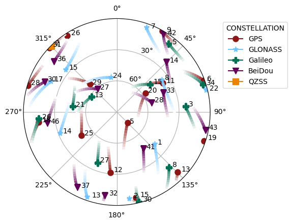
Figure 1: Over 48 positioning, navigation, and timing satellites are in view over Denver, Colorado.

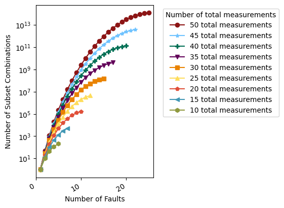
Figure 2: Number of subset combinations required by solution separation FDE depending on the number of measurements and faults.

Another FDE approach removes the combinatorial computation time of fault detection and exclusion by using a mathematical tool called Euclidean distance matrices (EDMs). This EDM FDE method has previously been shown to run using less compute time while maintaining high accuracy in both detecting and excluding faults [knowles_navigation]. Additionally, EDM FDE does not explicitly require an estimate of the receiver’s position to be able to perform FDE.

In the last two years since EDM FDE was originally presented, we have extensively tested the algorithm across multiple GNSS datasets. Additionally, we have gained additional insight into the mathematical basis for the algorithm by further inspecting the impact on the rank properties of EDMs when an EDM is constructed from faulty versus non-faulty signals. In this paper, we present a novel EDM FDE method that rapidly removes multiple faults by greedily removing the single satellite with the largest bias/fault in each iteration. Similar to greedy residual FDE, our EDM algorithm is also called greedy since it takes a locally optimal decision to remove the satellite with the largest bias/fault in each iteration in hopes of finding the globally optimal solution [greedy_algorithms]. We rigorously validate the advantages of the greedy EDM FDE method over a comparable greedy residual FDE method. This paper is based on our ION GNSS+ conference paper [knowles2023detection] but adds experimental results on a real-world dataset, additional insight on the impact of the receiver clock bias, and a detailed time complexity comparison against residual-based FDE and solution separation FDE in Section 6.

We first present a brief background on Euclidean distance matrices used for GNSS fault detection and exclusion in Section 2. Next, we explain the details of the new greedy EDM fault detection and fault exclusion strategies in Section 3 and explicitly describe its main differences over previously proposed EDM FDE methods [knowles_navigation]. In Section 4, we describe a simulated dataset we created to compare our greedy EDM FDE method with greedy residual FDE in terms of computation time and fault exclusion accuracy. In Section 5, we compare greedy residual FDE and our previous version of EDM FDE [knowles_navigation, githuboldedm] on a real-world dataset. Using the real-world dataset, we present results on computation time and localization accuracy for each method after excluding faulty measurements. Both greedy EDM FDE and greedy residual FDE are implemented within the open-source GNSS Python library gnss_lib_py [knowles2023gnss, knowles2022modular] which allows users to easily test the FDE methods on their own GNSS data. Section 6 provides a detailed theoretical runtime comparison between greedy EDM FDE, greedy residual FDE, and solution separation FDE. Finally, Section LABEL:sec:mods describes several possible modifications to greedy EDM FDE to change performance characteristics. The source code for all experiments and figures are available open source [githubgreedy].

2 Euclidean Distance Matrix Background

Euclidean distance matrices are a mathematical tool used for signal processing and obtaining information from distances [Dokmanic2015]. If constructed in a specific manner, Euclidean distance matrices are also able to check for GNSS signal faults thanks to a special rank property the matrices possess. By definition, Euclidean distance matrices contain the squared distances between all sets of points in a system. Figure 3 shows a visualization of how a Euclidean distance matrix is formed for a simple system comprised of three satellites and a single receiver. The distances between satellites are calculated using satellite ephemeris and the distances between the satellites and receiver are provided through the pseudorange measurement. A more complete background of Euclidean distance matrices and their relevance for GNSS fault detection is found in [knowles_navigation].

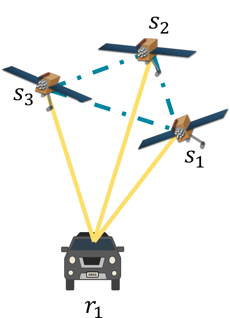
(a)

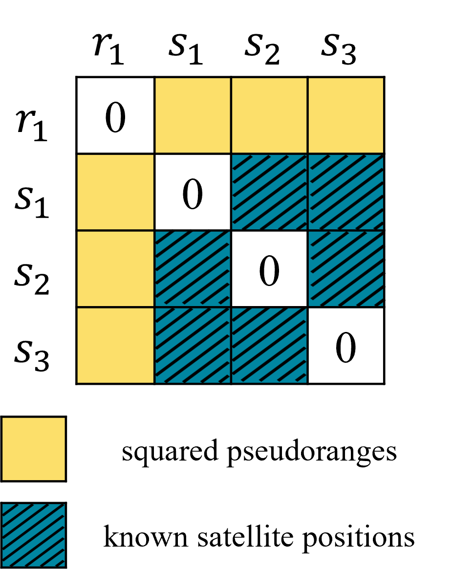
(b)

Figure 3: A combination of squared pseudoranges and known satellite positions are used to construct the EDM shown in subfigure (b) for the system shown in subfigure (a) of a single receiver and three satellites. Subfigure (b) taken from [knowles_navigation].

Once we construct the EDM, D, using processed pseudoranges and known satellite positions, we retrieve its corresponding symmetric Gram matrix, G, by double centering the EDM through Equation (1) where I represents the identity matrix, 1 is a column vector of ones, and $n$ is three — the dimension of the space spanned by the points in the system. For more information on recovering a Gram matrix through double centering, refer to ([Dattorro], section 5.4.2.2).

$$\text{{G}}=-\frac{1}{2}\textbf{J}\text{{D}}\textbf{J}\text{\quad where }\textbf{J}=\textbf{I}-\frac{1}{n}\textbf{1}\textbf{1}^{\top}.$$ (1)

If all distances are perfectly consistent, then the Gram matrix, G, has rank equal to the dimension of the state space [Horn1985]. In the case where we are solving for a three-dimensional receiver position, the state space has dimension of three, i.e. $n=3$. We explain in Section 3 how the rank of the Gram matrix, G, changes when there are faulty measurements inconsistent with the rest of the measurements.

3 Approach

In this section, we explain our approach for using EDMs to perform fault detection and exclusion. Our approach uses the particular geometry of the GNSS positioning problem to apply Euclidean distance matrices in a novel manner. This approach uses a different fault detection test statistic and fault exclusion strategy than previous work in [knowles_navigation]. The FDE approach has been drastically simplified thanks to increased understanding of EDMs and their use for fault detection and exclusion. In Section 3.1, we explain our EDM fault detection approach and in Section 3.2, we explain our greedy EDM fault exclusion approach. In Section 3.3 we explicitly describe the improvements of this work over previous EDM FDE methods, and in Section 3.4 we illustrate how all experiments can be reproduced.

3.1 Fault Detection

The key detail for using the recovered Gram matrix for fault detection is understanding how the eigenvalues of the Gram matrix change when faults are present in the measured pseudoranges used to construct the GNSS EDM. With increasing fault magnitude, the following happens to the eigenvalues as ordered from largest to smallest:

1. The first $n$ eigenvalues remain a consistent value. See Section 2 for the definition of $n$.

2. The $n+1$ and $n+2$ eigenvalues increase together as a pair.

3. The $n+3$ and all subsequent eigenvalues remain a consistent value.

The eigenvalues of the Gram matrix are an indication of its rank. When the $n+1$ and subsequent eigenvalues are nearly zero, that is an indication that the Gram matrix is close to having a rank of $n$. In Section 2, we clarified that all valid Gram matrices should have rank of $n$. When a fault is present in the pseudorange measurements and the $n+1$ and $n+2$ eigenvalues increase together as a pair, that means that the Gram matrix has rank of $n+2$ instead of rank $n$ as we expected.

One main insight and difference over previous work is to use the pair of the $n+1$ and $n+2$ eigenvalues for the fault detection test statistic. Since neither the first $n$ nor the $n+3$ and subsequent eigenvalues change significantly with increasing fault magnitude, none of those eigenvalues should be used for fault detection. The new fault detection test statistic is shown in Equation 2.

$$\frac{\lambda_{n+1}+\lambda_{n+2}}{2\lambda_{1}}>\text{detection threshold}$$ (2)

The EDM fault detection test statistic averages the $n+1$ and $n+2$ eigenvalues and divides by the largest eigenvalue to normalize the test statistic between zero and one and make the test statistic relatively agnostic to the amount of natural noise in the pseudorange measurements. If the test statistic is larger than the provided threshold then the measurements are deemed inconsistent and a fault is predicted within the measurements. However, if the test statistic is smaller than the provided threshold, then the measurements are deemed consistent and no faults are predicted within the measurements. The threshold is set by the user based on the natural noise present in the receiver’s pseudorange measurements. With increasing natural noise in the pseudorange measurements, the detection threshold should also increase so as to not remove non-faulty measurements.

The proposed fault detection test statistic works even when zero mean Gaussian noise is present in the pseudorange measurements. Figure 4 shows an example of a timestep with $n=3$ and 20 received satellite measurements. With zero mean Gaussian noise added to all the pseudoranges, the fourth and fifth eigenvalues are nonzero even when there are no faults present in the pseudoranges. However, when even a single fault exists in the measurements, the fourth and fifth eigenvalues still drastically jump an order of magnitude. This means that even in the presence of noisy pseudorange measurements, we can still accurately detect the existence of faulty signals by detecting a jump in the value of the fourth and fifth eigenvalues.

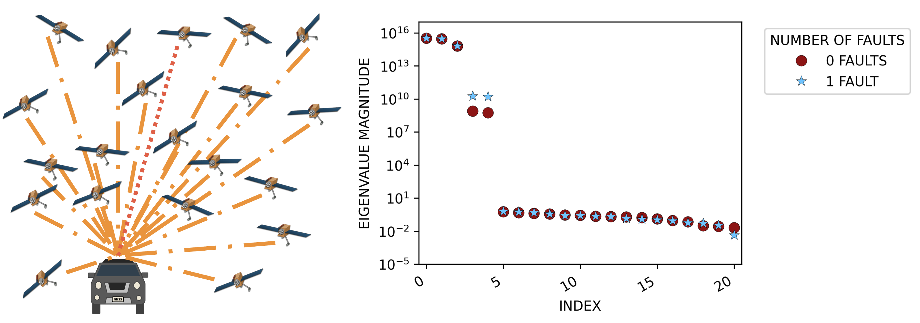
Figure 4: Even with noise, a single faulty bias added to a measurement dramatically increases the fourth and fifth eigenvalue of the Gram matrix.

3.2 Fault Exclusion

For fault exclusion, we inspect the eigenvectors associated with both the $n+1$ and $n+2$ eigenvalues. The intuition is that our fault exclusion strategy identifies the satellite measurements that are most influencing the increasing magnitude of the $n+1$ and $n+2$ eigenvalues. In implementation, we take the absolute value of the $n+1$ and $n+2$ eigenvectors and then take the elementwise average across the two vectors. The measurement with the largest average absolute value is predicted to be a measurement fault. Figure 5 shows an example of the absolute value of the eigenvectors, Q, obtained through eigenvalue decomposition of the Gram matrix, G, with $n=3$. In the example measurements, there exists a single measurement fault from the fourth satellite, $s_{4}$. The measurements from the fourth satellite produce the largest absolute values in the fourth and fifth eigenvectors indicating that it is the cause of the detected fault. Note that the first row of the Q matrix shown in Figure 5 corresponds to the receiver’s index since the EDM was constructed according to the order shown in Figure 3. The first row also has a relatively large absolute value magnitude indicating the fact that the receiver’s position is directly influenced by the faulty satellite pseudorange measurement.

Similar to greedy residual FDE’s approach of greedily removing the measurement with the largest normalized residual in each iteration [blanch2015fast], our greedy EDM FDE algorithm greedily chooses the satellite measurement to remove at each iteration with the largest effect on the $n+1$ and $n+2$ eigenvectors. This greedy removal of satellite measurements happens iteratively until the fault detection test statistic falls below the provided threshold. Algorithm 1 shows the full greedy EDM FDE algorithm.

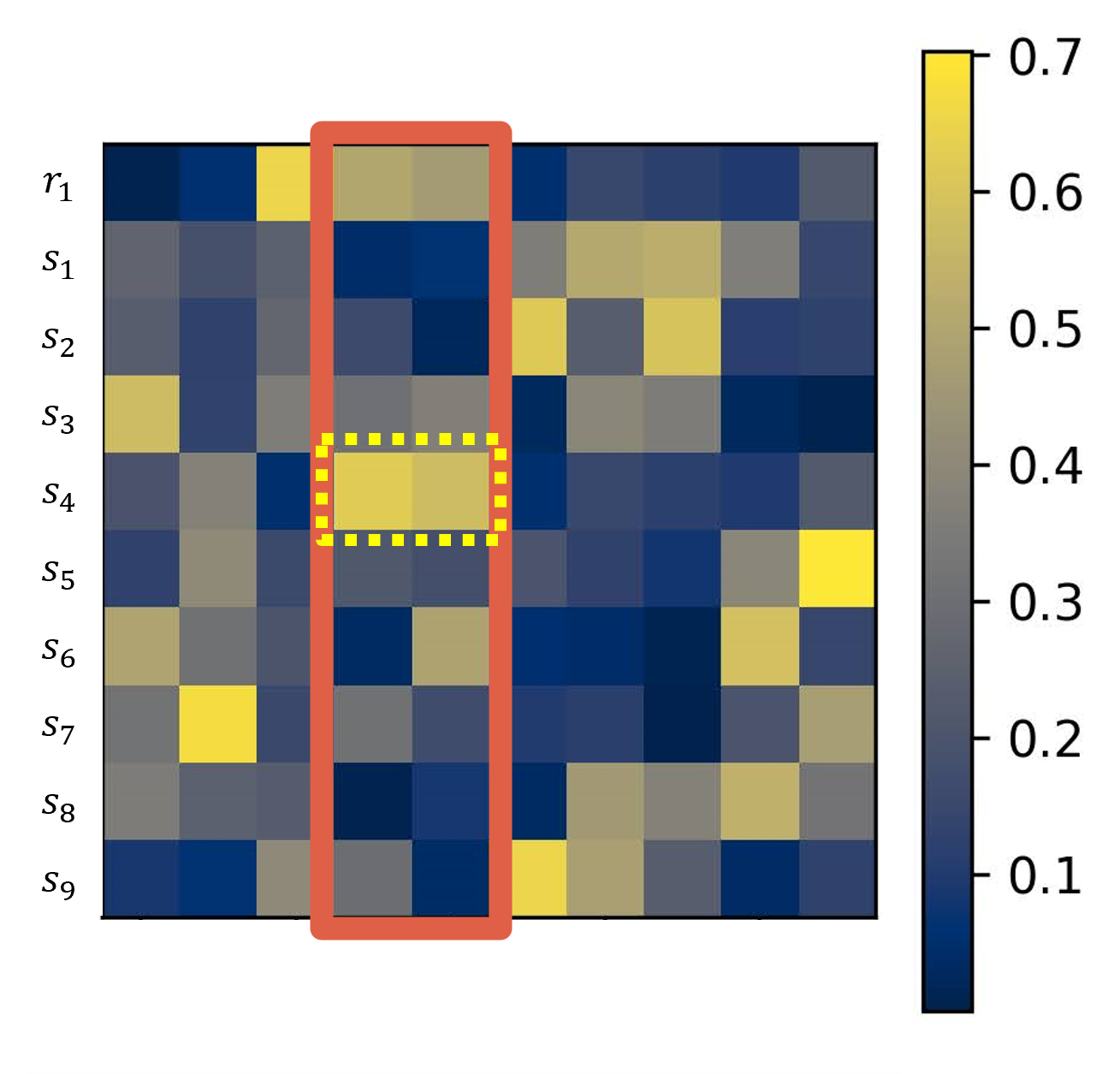
Figure 5: Eigenvectors, Q, of the Gram matrix, G.

Algorithm 1 Greedy EDM FDE

1:Inputs:

2:     $n$ : Dimension of state space

3:     D: Euclidean distance matrix

4:     $T_{d}$ : detection threshold

5:Initialize:

6:     G$\leftarrow-\frac{1}{2}\textbf{J}\text{{D}}\textbf{J}$

7:     $\textbf{Q},\bm{\Lambda}\leftarrow\text{EVD}(\text{{G}})$

8:while # satellites $>$ 4 do

9:     if $(\lambda_{n+1}+\lambda_{n+2})/(2\lambda_{1})<T_{d}$ then

10:         break

11:     end if

12:     index $\leftarrow\max\left(\left|(q_{n+1}+q_{n+2})/2\right|\right)$

13:     exclude index from D

14:     $\text{{G}}\leftarrow-\frac{1}{2}\textbf{J}\text{{D}}\textbf{J}$

15:     $\textbf{Q},\bm{\Lambda}\leftarrow\text{EVD}(\text{{G}})$

16:end while

3.3 Improvements over Previous EDM FDE Methods

The approach described in Section 3.1 and Section 3.2 is a significant improvement over our prior work in [knowles_navigation]. Throughout the rest of the paper, we refer to our previous EDM FDE algorithm as our EDM 2021 algorithm since that was the year in which the method was originally published [githuboldedm]. Our EDM 2021 algorithm used Equation 3 for the fault detection test statistic where $m$ is the total number of measurements available.

$$\frac{\lambda_{n+1}\times\frac{1}{m-n}\sum^{m}_{i=n+1}\lambda_{i}}{\lambda_{1}}>\text{detection threshold}$$ (3)

Based on new experience working with EDM matrices, we discovered the relationship shown in Figure 4 that the $n+1$ and $n+2$ eigenvalues increase together as a pair when a fault is present. While Equation 3 from previous work multiplied the $n+1$ and the average of the $n+1$ to $m$ eigenvalues, we now know that the $n+3$ and subsequent eigenvalues remain a consistent value so their magnitudes do not add significance to test statistic. Hence, in our updated test statistic shown in Equation 2, we only look at the average of the $n+1$ and $n+2$ eigenvalues which affords a more clear signal to recognize faults with the test statistic.

Another significant improvement over prior work is the simplicity of the new fault exclusion approach. The simple method from Algorithm 1 can be implemented directly with accurate detection performance. The EDM 2021 implementation of the algorithm used a complex check iterating through possible candidates of both the maximums and minimums of the left and right singular vectors of the Gram matrix [githuboldedm]. Based on our new experience, we now know to inspect the absolute value of the $n+1$ and $n+2$ eigenvectors which dramatically simplifies the implementation of Algorithm 1 which is available open source [githubgreedy].

Finally, in this work we test against both simulated and a real-world dataset with the algorithm fully implemented in an open-source library. All of our results are reproducible as described in Section 3.4.

3.4 Algorithm Reproducibility

To enable the reproducibility of all experiments, both greedy EDM FDE and the baseline comparison of greedy residual FDE have been implemented in our open-source GNSS Python library gnss_lib_py [knowles2023gnss, knowles2022modular]. Figure 6 shows that with just a few lines of code, users can upload data from the Google Smartphone Decimeter Challenge 2023 [smartphone-decimeter-2023] and then perform either EDM or residual FDE simply by changing the method input parameter to the function call. The output of the function returns a one if a fault is predicted and a zero if no fault is predicted for each satellite measurement in the dataset.

For more detailed instructions, tutorials are available on how to use the gnss_lib_py library and its associated FDE functions at gnss-lib-py.readthedocs.io. All specific code to run the experiments in Section 4 and Section 5 as well as generate the included figures is also open source [githubgreedy].

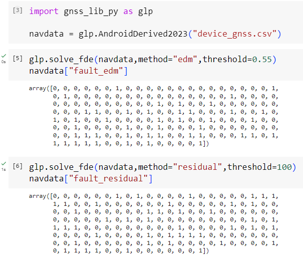
Figure 6: Example function calls to run either EDM FDE or residual FDE.

4 Simulated Dataset Results

To initially validate our greedy EDM FDE approach, we created a simulated dataset using nine global locations: Calgary, Canada; Cape Town, South Africa; Hong Kong; London, United Kingdom; Munich, Germany; Sao Paulo, Brazil; San Francisco, USA; Sydney, Australia; and Zurich, Switzerland. At each location, we simulated measurements at five minute intervals across a time span of 24 hours. We used the open-source library gnss_lib_py [knowles2023gnss] to obtain satellite locations given a specific timestamp and receiver location. For three of the locations — Calgary, London, and Zurich — we used an elevation mask of 30 degrees to remove measurements near the horizon and for all other locations we used an elevation mask of 10 degrees.

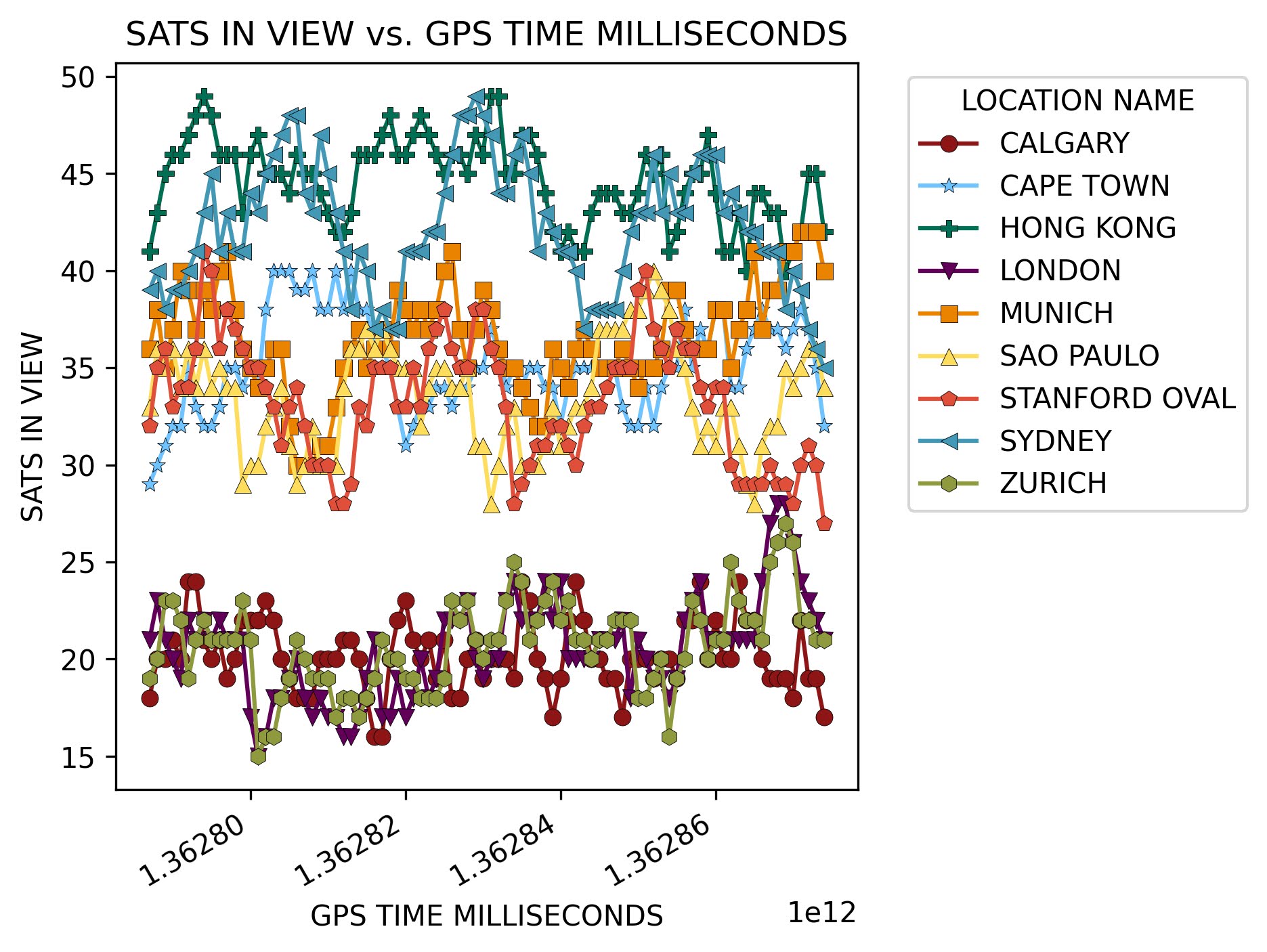
Figure 7: Number of satellites in view across the dataset.

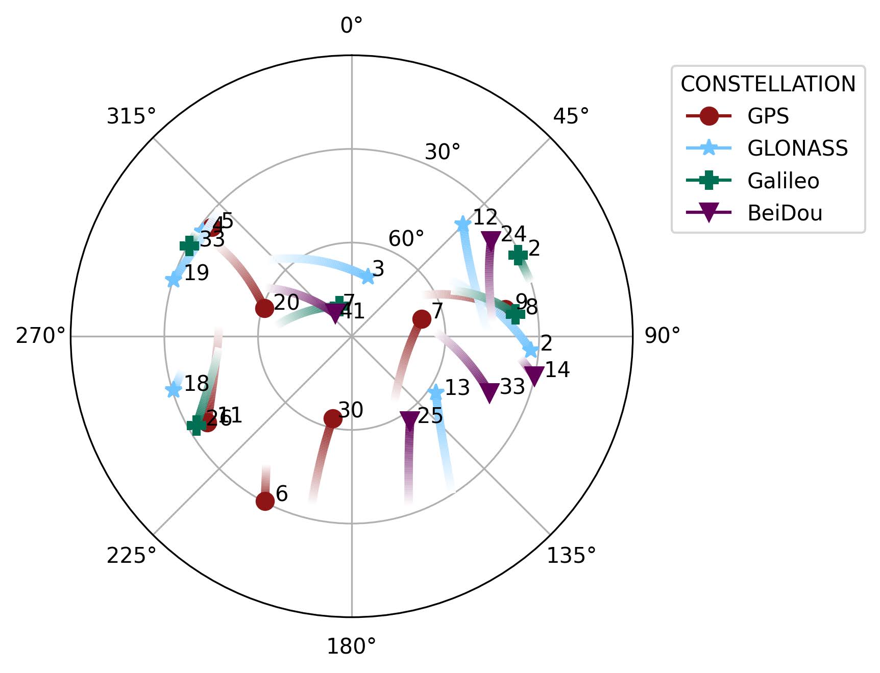
Figure 8: Skyplot of a section of the simulated data from Zurich.

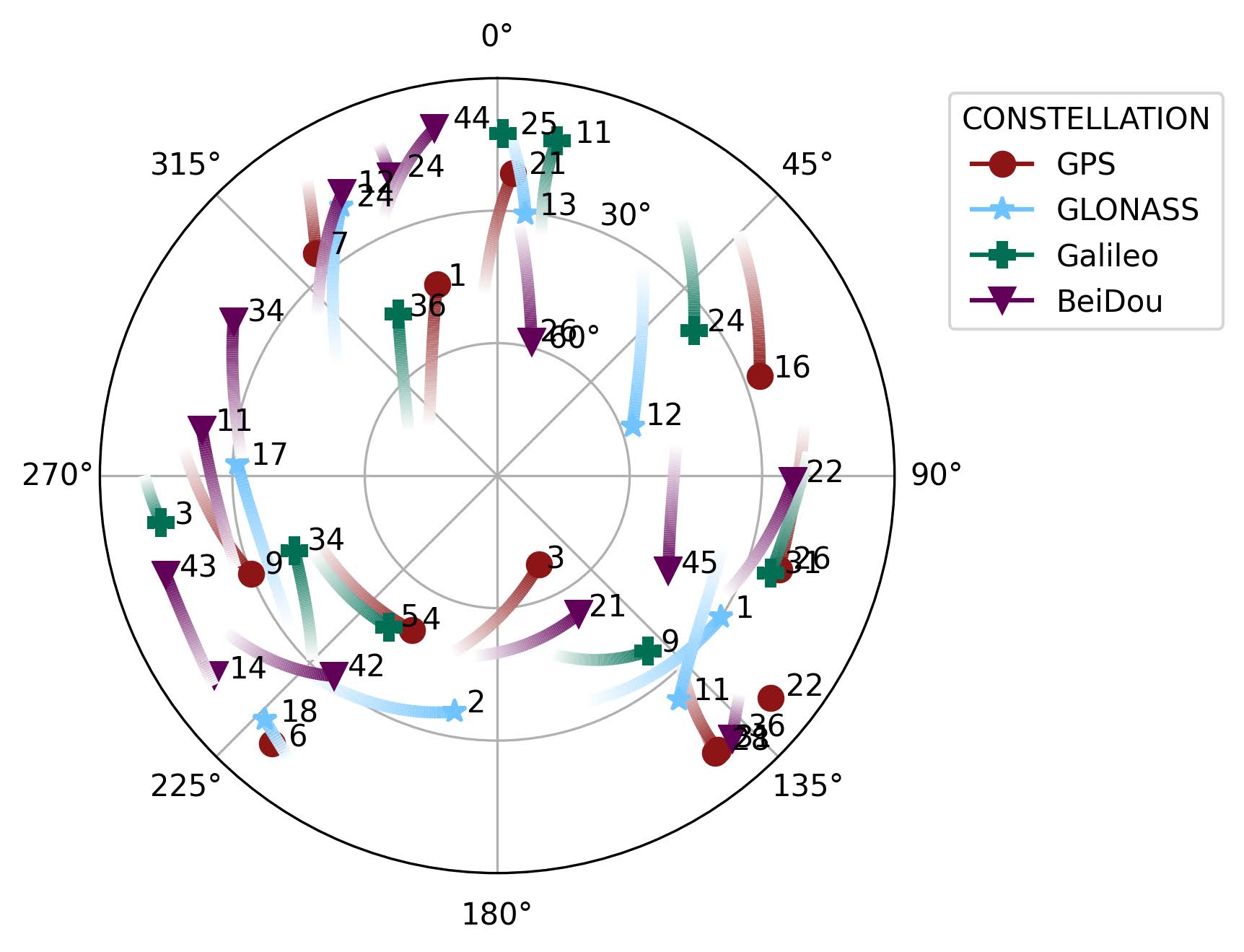
Figure 9: Skyplot of a section of the simulated data from Sao Paulo.

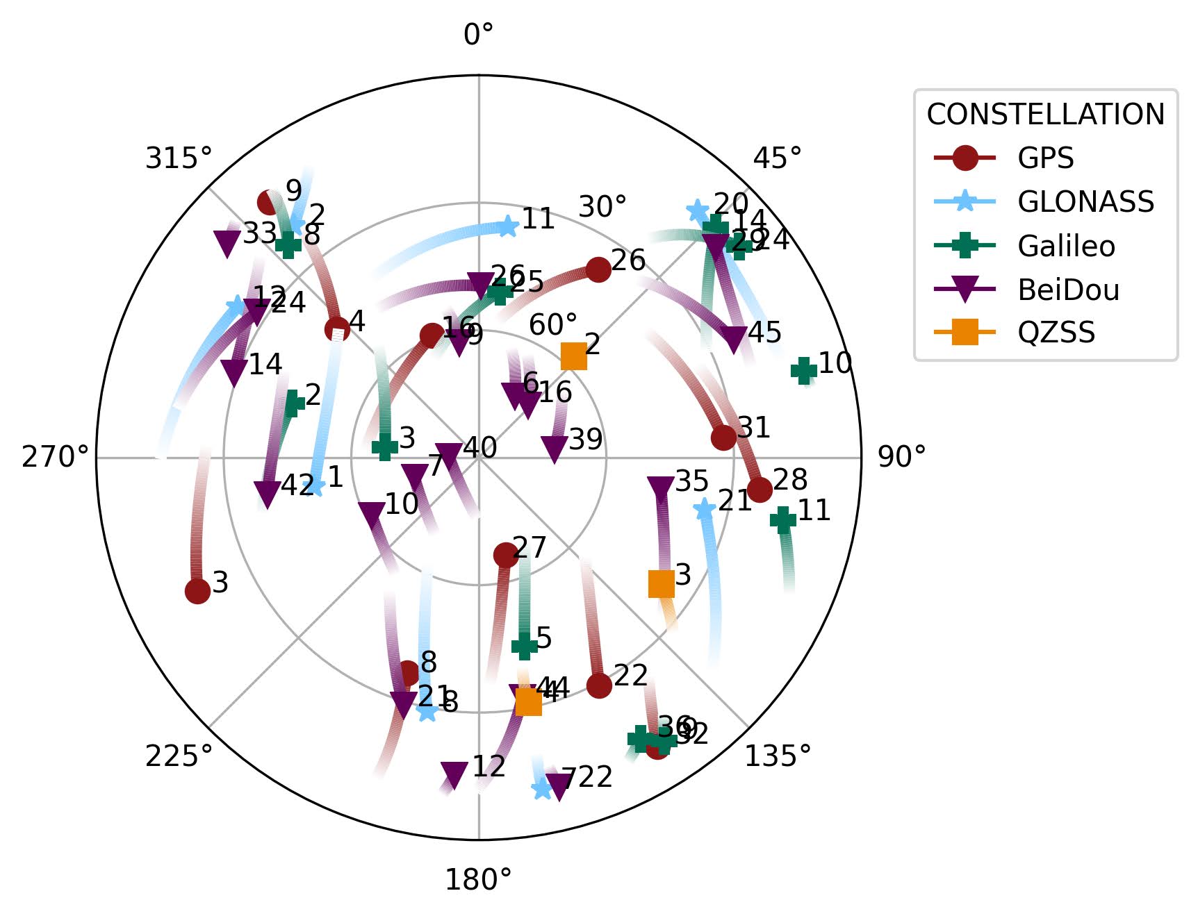
Figure 10: Skyplot of a section of the simulated data from Hong Kong.

Figure 7 shows the resulting number of satellites in view at each location across the dataset. The Calgary, London, and Zurich locations have fewer satellites in view due to the larger elevation mask. In total, the simulated dataset creates 2,601 different satellite geometries to test against. Figures 8, 9, and 10 show the varied satellite geometries in our simulated dataset from Zurich, Sao Paulo, and Hong Kong respectively. Zero mean gaussian noise with a standard deviation of 10m was added to all measurements. Biases of 10, 20, 40, and 60 m were added to either 1, 2, 4, 8, or 12 measurements at each timestep depending on the parameters of the test.

To validate the proposed greedy EDM FDE algorithm, we compare it against greedy residual FDE on our simulated dataset. In the Section 4.1, we present results of the computation time and in Section 4.2, we present fault exclusion accuracy results. Our results validate the rapid computation time of the greedy EDM FDE algorithm in the presence of many measurements and many faults when compared with greedy residual FDE.

4.1 Computation Time Analysis

Greedy EDM FDE outperforms greedy residual FDE in terms of computation time. Figure 11 shows that greedy EDM FDE runs on average faster than greedy residual FDE in the presence of increasing number of measurements. Figure 12 shows that greedy EDM FDE also runs on average faster than greedy residual FDE in the presence of increasing number of faults. In both Figure 11 and 12 one standard deviation on either side of the mean computation time is shaded indicating the variability present in the computation time results. In addition to the experimental results shown in this section, Section 6 derives the theoretical time complexity for EDM FDE, residual FDE, and solution separation.

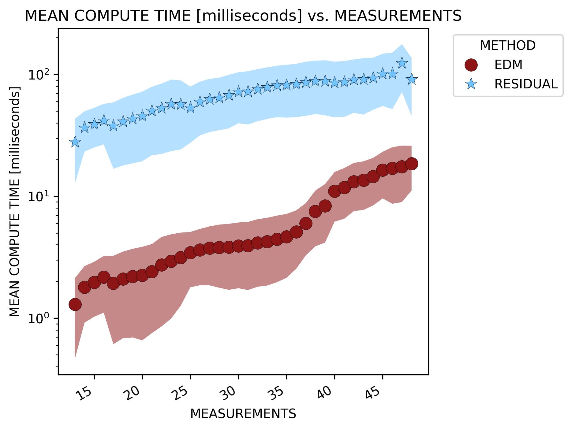
Figure 11: Mean computation time of greedy EDM and greedy residual FDE with increasing number of measurements. One standard deviation on either side of the mean is shaded.

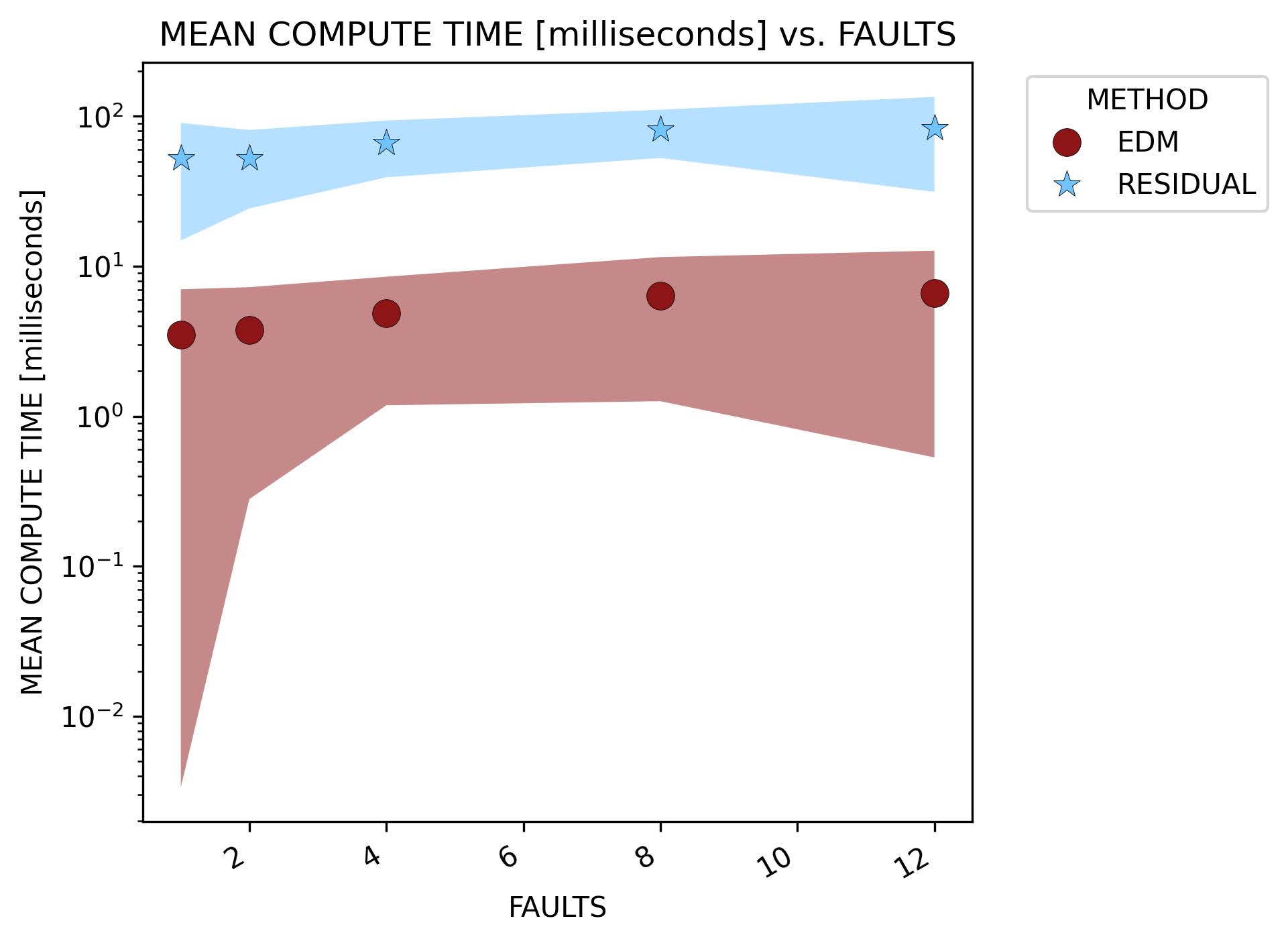
Figure 12: Mean computation time of greedy EDM and greedy residual FDE with increasing number of faults. One standard deviation on either side of the mean is shaded.

4.2 Fault Exclusion Accuracy

Our measure for fault exclusion accuracy uses the receiver operating characteristic (ROC) curve. Figure 13 shows the ROC curves for both greedy EDM and greedy residual FDE for a scenario with eight faults at the Munich location and varying fault magnitudes. The ROC curve is created by sweeping across a range of threshold parameters and shows how the true positive rate (the percentage of faulty measurements correctly identified) increases as the false alarm rate (percentage of non-faulty measurements incorrectly identified as faulty) increases. An algorithm is deemed to be more accurate at excluding faults if the curve goes towards the top left corner of the graph. Figure 13 shows that both algorithms are better at detecting faults as the magnitude of the fault increases above the noise floor of the 10m zero mean Gaussian noise added to all measurements. Figure 13 also shows that greedy EDM and greedy residual FDE perform nearly identically for each fault bias magnitude. A single quantitative metric from the ROC curve is calculated as the area under the curve (AUC) for each scenario. A larger AUC means the method is better at excluding faults.

In Table 1, we show the area under the curve for all locations and two conditions of a single 20m fault bias and eight 60m fault biases. The area under the curve (AUC) is comparable for both greedy residual and greedy EDM FDE illustrating the fact that greedy EDM FDE is able to achieve comparable performance in terms of fault detection accuracy across the dataset when compared to greedy residual FDE. As described in Section 4 and displayed in Figure 7, the Calgary, London, and Zurich locations were created using a larger elevation mask leaving fewer visible satellites. Since those locations have fewer total measurements, the AUC at those locations is lower when eight measurements are faulty because there are fewer measurements available to create a consistent fault-free measurement set.

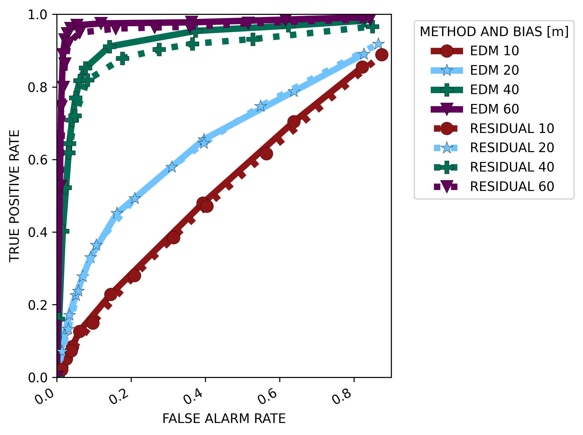
Figure 13: The receiver operating characteristic (ROC) curve for both greedy EDM FDE and greedy residual FDE across four different fault bias magnitudes.

Table 1: Area under the receiver operating characteristic (ROC) curve for both greedy EDM and greedy residual FDE.

			Area Under ROC Curve
Location	Fault Bias [m]	# Faults	Greedy EDM	Greedy Residual
Calgary	20	1	0.44	0.44
Cape Town	20	1	0.51	0.48
Hong Kong	20	1	0.50	0.48
London	20	1	0.42	0.43
Munich	20	1	0.49	0.48
Sao Paulo	20	1	0.52	0.51
Stanford Oval	20	1	0.51	0.49
Sydney	20	1	0.51	0.52
Zurich	20	1	0.46	0.47
Calgary	60	8	0.26	0.30
Cape Town	60	8	0.67	0.65
Hong Kong	60	8	0.69	0.70
London	60	8	0.28	0.33
Munich	60	8	0.68	0.67
Sao Paulo	60	8	0.67	0.66
Stanford Oval	60	8	0.67	0.66
Sydney	60	8	0.69	0.69
Zurich	60	8	0.27	0.32

5 Real World Data Results

To further validate the proposed greedy EDM FDE algorithm, we also compare our algorithm against greedy residual FDE and our previous 2021 version of EDM FDE on the Google Smartphone Decimeter Challenge (GSDC) 2023 [smartphone-decimeter-2023]. We use a subset of the total dataset by taking the 68 urban traces from seven different android phones that include multipath indicators. This dataset consistently provides 25-45 satellite measurements at each timestep epoch. In Section 5.1 we present results of the compute time on the real-world data and in Section 5.2 we provide results on the localization accuracy achievable using either our new greedy EDM FDE method, residual FDE, or our previous 2021 EDM FDE algorithm.

Since EDM FDE is reliant on matching distances between pairs of points, EDM FDE works best if those distances are as close to their truth value as possible. Unlike when using the simulated data in Section 4, when using real-world data, we first condition the pseudorange by removing known biases from the measured pseudorange using the equation:

$$\rho=\rho_{m}+b_{rx}-I+T-c_{b},$$ (4)

Where $\rho_{m}$ is the measured pseudorange, $b_{rx}$ is the receiver’s clock bias, $I$ is the Ionosphere delay, $T$ is the Troposphere delay, and $c_{b}$ is the constellation bias. In the results that follow, we estimated the receiver clock bias using weighted least squares and the atmospheric and constellation bias are provided in the GSDC dataset itself.

5.1 Computation Time

Greedy EDM FDE outperforms greedy residual FDE in terms of computation speed by an order of magnitude when averaged across all 68 real-world data traces. Figure 14 shows the average computation time for all FDE methods with increasing number of measurements at each timestep. One standard deviation on either side of the mean is shaded on the plot. This plot justifies the fact that Greedy EDM FDE can rapidly remove multiple faults in the presence of many measurements. Both our new EDM FDE method presented in this paper and our previous 2021 version of EDM FDE perform similarly in terms of computation speed.

Since both EDM FDE and residual FDE algorithms greedily remove faults, the computation time of both algorithms is not only a factor of the number of measurements but also the number of faults predicted. If the threshold for either algorithm is set low, then the algorithm will more often enter the fault exclusion step and iterate again to remove more satellite measurements. If the threshold for either algorithm is set high, then the algorithm will rarely enter the fault exclusion step nor iterate to remove additional measurements. To remove the effect the threshold value has on computation time, for each trace, we used the computation time of the threshold that minimized the accuracy metric we describe in Section 5.2.

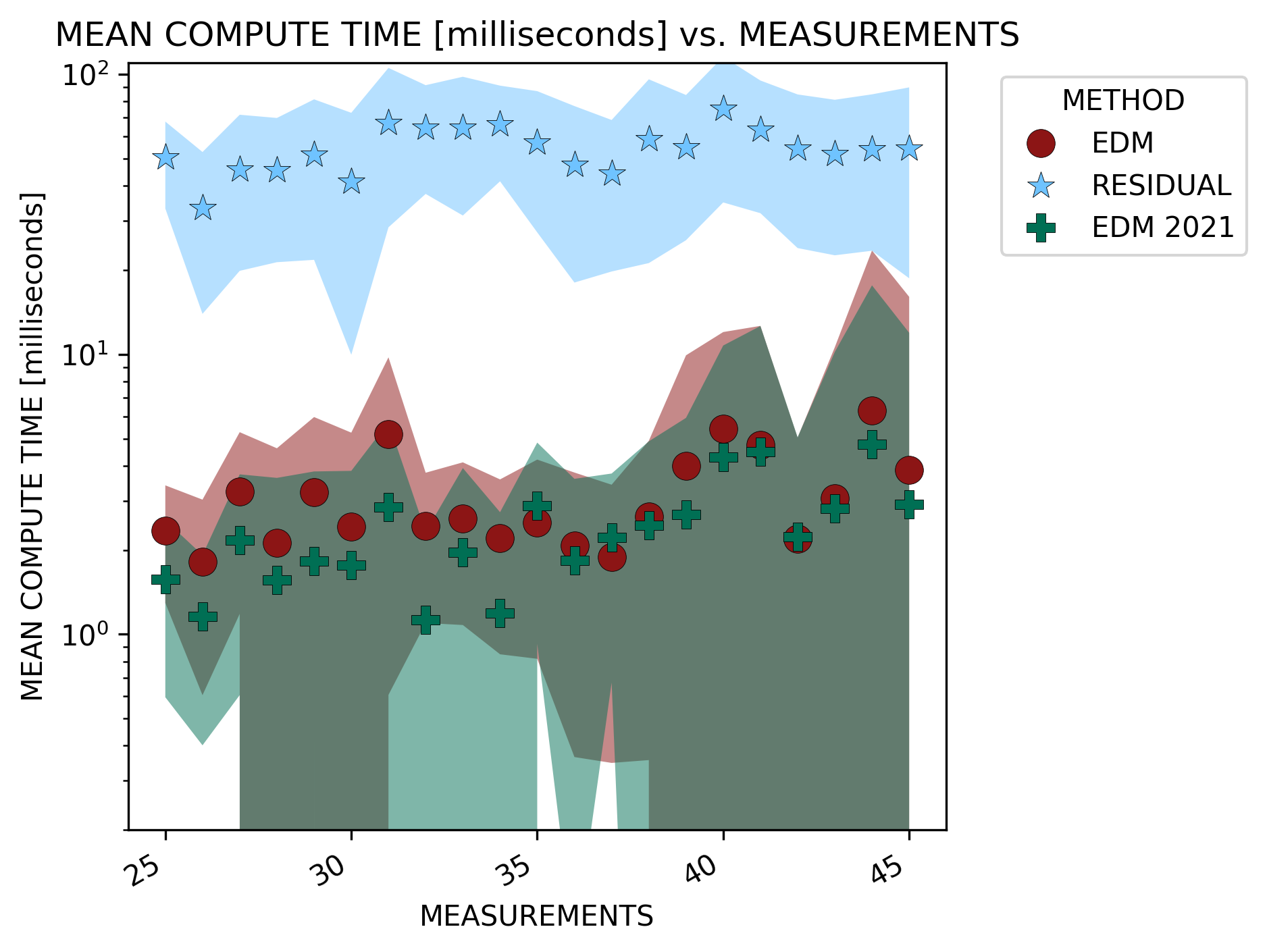
Figure 14: Mean computation time of greedy EDM and greedy residual FDE with increasing number of measurements. One standard deviation on either side of the mean is shaded.

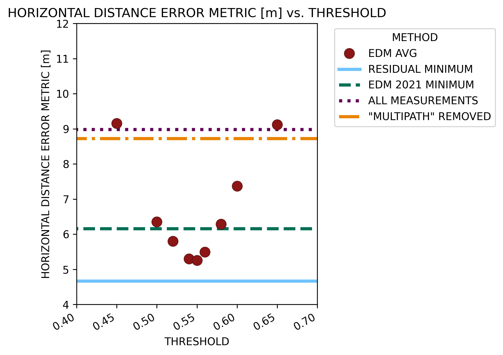
Figure 15: Horizontal distance error metric for multiple choices of the EDM FDE threshold.

5.2 Localization Accuracy

In the real world, there is no clear consensus of what constitutes a “faulty” satellite measurement. The GSDC dataset includes indicators of whether the android operating system deemed the satellite measurement to be multipath, but provides no information on whether measurements came from line-of-sight satellites, etc. To avoid rigidly defining “faults” as multipath, non-line-of-sight, or something else, we abstract away satellite level faults and instead focus on the localization accuracy using the predicted non-faulty measurements.

The GSDC 2023 dataset provides a “ground truth” position at each timestep [smartphone-decimeter-2023]. For each algorithm, we predict which satellite measurements are faulty, then run weighted least squares to estimate the receiver’s position with the non-faulty measurements. We then use the same horizontal distance error metric as the GSDC [smartphone-decimeter-2023] by computing the 50th and 95th percentile horizontal distance error of the weighted least squares solution when compared with the GSDC “ground truth” for each trace. The 50th and 95th percentiles are then averaged together to reduce to a single value for each trace. We perform this process for each of the 68 real-world traces and then average this horizontal distance error metric across all the traces. We repeat this method sweeping across a range of threshold values for each algorithm.

Figure 15 shows the horizontal distance error metric for our new EDM FDE algorithm across a range of threshold values from 0.45 to 0.65. The plot shows that using EDM FDE achieves the lowest errors when the threshold value is set to the middle of that range near 0.55. If the threshold is too high, then missed detections result in larger errors. If the threshold is set too low, then too many satellite measurements are removed thus degrading the geometry of the localization problem and increasing error. The plot also compares against weighted least squares using all measurements and using all measurements which the android operating system has deemed are not multipath measurements. EDM FDE is thus shown to decrease horizontal position errors by correctly removing faulty satellite measurements. Figure 15 also plots the minimum error achievable with the other two FDE algorithms of greedy residual FDE and our previous 2021 version of EDM FDE. The plot shows that our new version of EDM FDE from this paper is able to outperform our previous 2021 version of EDM FDE. In Section 3.3 we described our change to the fault detection test statistic that provides a more clear indication of measurement faults despite noise in the measurements. Thus, our new version of EDM FDE from this paper is able to more accurately remove faults in the noisy GSDC dataset and achieve a lower localization error than our previous 2021 version of EDM FDE.

Figure 16 shows the horizontal distance error metric when using residual-based FDE for threshold values from 10 to 100,000 and Figure 17 shows the horizontal distance error metric when using our previous 2021 version of EDM FDE for threshold values from 0.3 to 300. Greedy residual FDE is able to achieve the lowest horizontal position errors with a well-chosen threshold and our previous 2021 version of EDM FDE has the largest horizontal distance errors out of the three algorithms we tested even with the best threshold values. Figures 15– 17 do show that no matter the FDE method, lower horizontal distance errors are possible by removing faults versus using all measurements or only removing the measurements that the android operating system indicated include multipath.

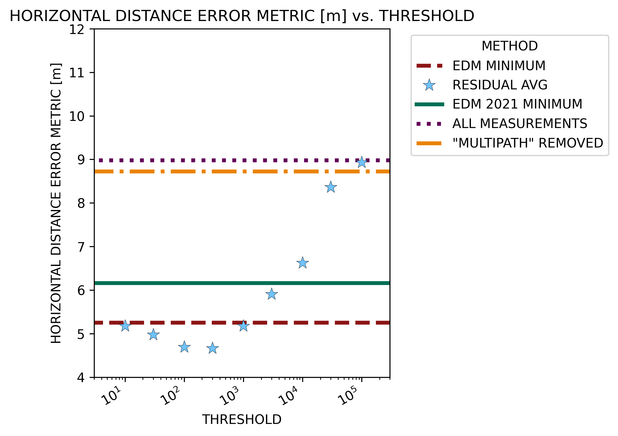
Figure 16: Horizontal distance error metric for multiple choices of the residual FDE threshold.

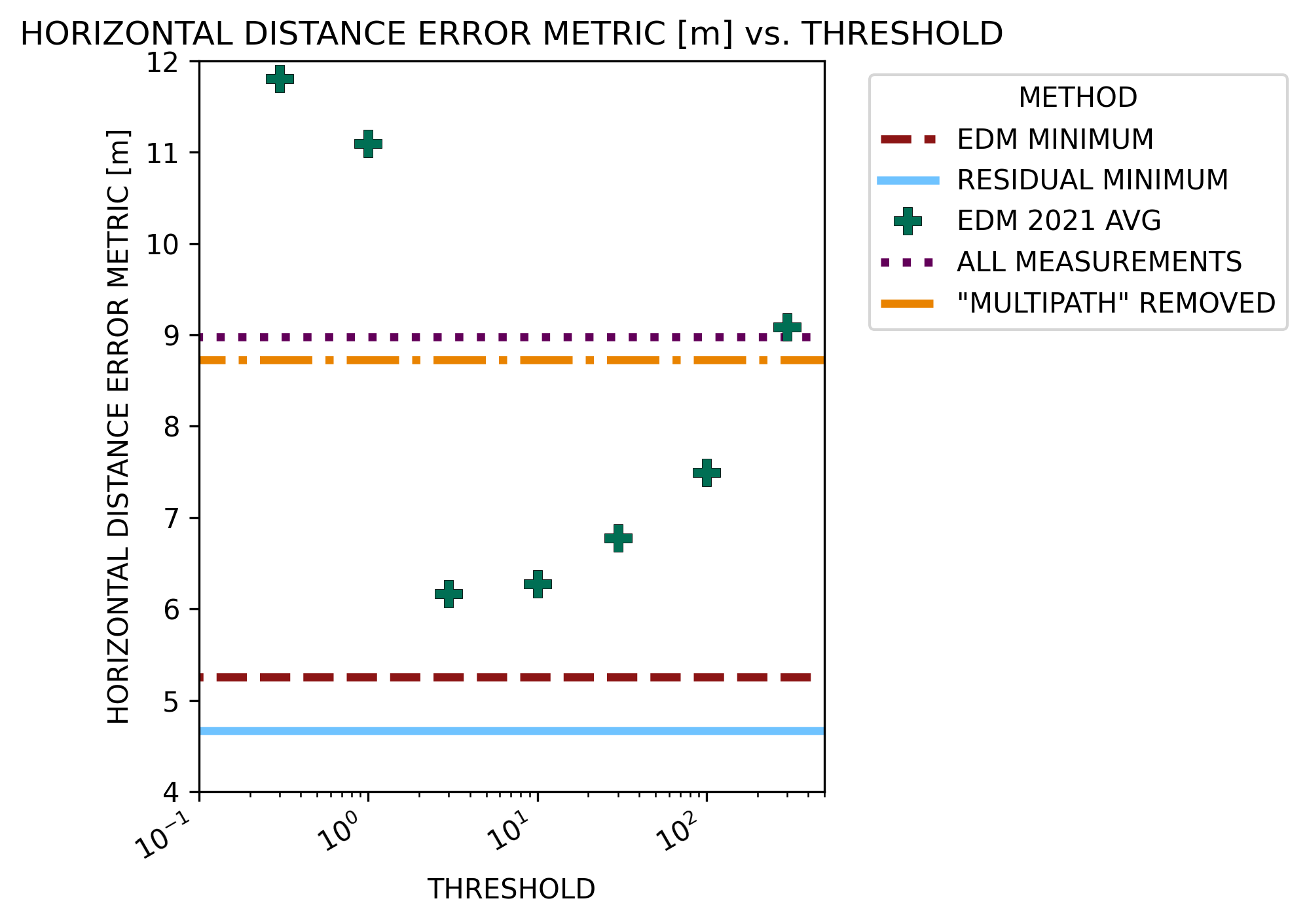
Figure 17: Horizontal distance error metric for multiple choices of the EDM 2021 threshold.

6 Time Complexity Derivations

This section presents a theoretical runtime complexity comparison for EDM FDE in Section LABEL:sec:edm_alg_time, residual FDE in Section LABEL:sec:residual_alg_time and solution separation in Section LABEL:sec:solution_separation_alg_time. We offer general remarks and a visual comparison to finalize in Section LABEL:app:final_compare. For ease of comparison, we use common notation found in Section 6.1 for all algorithms.

6.1 Nomenclature