A Fourier Approach to the Parameter Estimation Problem for One-dimensional Gaussian Mixture Models

Abstract

The purpose of this paper is twofold. First, we propose a novel algorithm for estimating parameters in one-dimensional Gaussian mixture models (GMMs). The algorithm takes advantage of the Hankel structure inherent in the Fourier data obtained from independent and identically distributed (i.i.d) samples of the mixture. For GMMs with a unified variance, a singular value ratio functional using the Fourier data is introduced and used to resolve the variance and component number simultaneously. The consistency of the estimator is derived. Compared to classic algorithms such as the method of moments and the maximum likelihood method, the proposed algorithm does not require prior knowledge of the number of Gaussian components or good initial guesses. Numerical experiments demonstrate its superior performance in estimation accuracy and computational cost. Second, we reveal that there exists a fundamental limit to the problem of estimating the number of Gaussian components or model order in the mixture model if the number of i.i.d samples is finite. For the case of a single variance, we show that the model order can be successfully estimated only if the minimum separation distance between the component means exceeds a certain threshold value and can fail if below. We derive a lower bound for this threshold value, referred to as the computational resolution limit, in terms of the number of i.i.d samples, the variance, and the number of Gaussian components. Numerical experiments confirm this phase transition phenomenon in estimating the model order. Moreover, we demonstrate that our algorithm achieves better scores in likelihood, AIC, and BIC when compared to the EM algorithm.

Keywords: Gaussian Mixture Models, parameter estimation, computational limit, model order selection.

1 Introduction

Mixture models[24, 9, 25] are widely used in various fields to model data and signals originating from sub-populations or distinct sources. Among mixture models, the Gaussian mixture model[33, 31] has emerged as one of the most extensively examined and widely applied models. This model finds utility in diverse domains, including optical microscopy, astronomy, biology, and finance. The probability density function of a mixture of k-Gaussian in $m$-dimensional space has the following form:

$$p(x)=\sum_{i=1}^{k}\pi_{i}g(x;\mu_{i},\boldsymbol{\Sigma}_{i})$$ (1.1)

where $g(x;\mu_{i},\boldsymbol{\Sigma}_{i})=(2\pi)^{-\frac{m}{2}}\det(\boldsymbol{\Sigma}_{i})^{-\frac{1}{2}}\exp\left({-\frac{1}{2}(x-\mu_{i})^{\mathrm{T}}\boldsymbol{\Sigma}_{i}^{-1}(x-\mu_{i})}\right)$ is the Gaussian density function and $0<\pi_{i}<1,\mu_{i}\in\mathbb{R}^{m},\boldsymbol{\Sigma}_{i}\in\mathbb{R}^{m\times m}$ are the weight, mean and covariance matrix of the $i$-th component of the mixture, respectively. A fundamental problem within the context of mixture models is the estimation of the component number and the parameters $(\pi_{i},\mu_{i},\boldsymbol{\Sigma}_{i})$ from given i.i.d samples of the mixture model.

The first approach to the parameter estimation of GMMs can be traced back to the work of Pearson in 1894[29], where he introduced method of moments to identify the parameters in his model. His idea is to equate the moments $\mathbb{E}[X^{i}]$ with the empirical moments calculated from the observed data $\frac{1}{n}\sum_{j=1}^{n}X_{j}^{i}$, which facilitated determining the unknown parameters through a system of equations. However, Pearson’s method is limited in practice due to its sensitivity to moment selection and constraints regarding specific moments, making it less applicable to heavy-tailed distributions and those lacking certain moment properties[32]. The drawbacks of the method of moments motivated various modifications including the Generalized Method of Moments[12], which minimizes the sum of differences between the sample moments and the theoretical moments. However, the generalized method of moments involves solving a nonconvex optimization problem, which may have slow convergence issues and a lack of theoretical guarantees. In [40], a denoised method of moments is proposed which denoises the empirical moments by projection onto the moment space[16]. Recent work based on the method of moments provides provable results for the Gaussian location-scale mixtures, see [15, 28, 3, 13].

With the development of computers and highly efficient numerical algorithms, maximum likelihood method has gained prominence as a widely adopted approach for parameter estimation problems. For a given mixture model with unknown parameters, the maximum likelihood method searches its parameters by maximizing the joint density function, or the so-called likelihood function of the observed data. Compared to the method of moments, the maximum likelihood method often achieves better estimations, especially in cases with large sample sizes.

Numerous iterative methods for optimization are proposed to seek the maximum or local maximum of the likelihood function [26]. The method of scoring proposed by Rao[30] in 1948 can be viewed as a variant of Newton’s methods. Among the maximum likelihood methods, the most commonly used one is the EM (Expectation Maximization) algorithm [8, 41, 7]. EM algorithm iterates a two-step operation to find a local maximum of the logarithm likelihood function, which may not necessarily be the ground-truth parameters. Due to this reason, it is common in practice to execute the EM algorithm multiple times with different initial values and select the result associated with the highest likelihood function value. For the convergence guarantees of EM algorithms under certain conditions, we refer to [6, 39]. Despite the slow convergence of the EM algorithm in some applications, the EM algorithm maintains popularity due to its straightforward implementation and minimal memory requirements[32]. For a more comprehensive discussion of the EM algorithm, we refer to [32, 4].

Bayesian approach can also be used for GMMs[23, 34]. This is achieved by specifying a prior distribution over the parameters of the model and then using Bayes’ theorem to update the prior distribution based on the observed data, as is in the variational Bayesian Gaussian mixture [5]. In addition to the Bayesian approach, a variety of sampling methods have been proposed for the estimation problem. This involves directly sampling from the joint distribution of the data and the parameters, using methods like Gibbs sampling[11] or Metropolis-Hastings sampling[27, 14]. Although these approaches are flexible and can be used for complex models, they are computationally intensive.

It is worth noting that both moment-based and maximum likelihood methods require prior knowledge of the component number $k$ in the mixture model. In practice, too many components may result in overfitting of data which makes it hard for interpretation. Fewer components make the model not enough to describe the data. Commonly used methods for determining the model order are based on the information criteria such as the AIC [1] and BIC [36]. These criteria select the model by introducing a penalty term for the number of parameters in the model. However, such an approach tends to favor overly simple models in practice. It remains elusive when they can guarantee that the model order estimation is correct.

1.1 Mathematical Model and Main Contributions

In this paper, we focus on the one-dimensional Gaussian mixture model with a unified variance that has the following probability density function:

$$p(x)=\sum_{i=1}^{k}\pi_{i}{g}(x;\mu_{i},s^{2}),$$ (1.2)

where $g(x;\mu,s^{2})=\frac{1}{\sqrt{2\pi s^{2}}}e^{-\frac{(x-\mu)^{2}}{2s^{2}}}$. In the above model, the mixture consists of $k$ components characterized by their means $\mu_{i}$’s, variance $s^{2}$, and weights $\pi_{i}$’s. We can also write

$$p(x)=g(x;0,s^{2})*\nu,$$ (1.3)

where $\nu=\sum_{i=1}^{k}\pi_{i}\delta_{\mu_{i}}(x)$ is called the mixing distribution. The parameter estimation problem is to estimate the component number $k$, the unified variance $s^{2}$, and mixing distribution $\nu$. For later use, we denote

$$\pi_{\min}=\min_{1\leq i\leq k}\left\lvert\pi_{i}\right\rvert,\quad d_{\min}=\min_{1\leq i\neq j\leq k}\left\lvert\mu_{i}-\mu_{j}\right\rvert.$$ (1.4)

In a departure from the method of moments and maximum likelihood methods, we propose to estimate the parameters by using the following Fourier data that can be obtained from samples of the mixture models

$$Y(\omega)=\hat{g}(\omega;s^{2})(\sum_{i=1}^{k}\pi_{i}e^{\iota\mu_{i}\omega}),$$ (1.5)

where $\hat{g}(\omega;s^{2})=e^{-\frac{s^{2}}{2}\omega^{2}}$ is the Fourier transform of $g(x;0,s^{2})$. Indeed, consider the following empirical characteristic function

$$Y_{n}(\omega)=\frac{1}{n}\sum_{j=1}^{n}e^{\iota\omega X_{j}},$$ (1.6)

where $n$ is the sample size and $X_{i}$ is the $i$-th sample. Assume that $X_{1},\cdots,X_{n}$ are independent samples drawn from the mixture model (1.2). The central limit theorem implies that

$$\sqrt{n}\left({Y}_{n}(\omega)-{Y}(\omega)\right)\xrightarrow{d}\mathcal{N}\left(0,1-\left\lvert{Y}(\omega)\right\rvert^{2}\right),\quad n\rightarrow+\infty,$$

where $\xrightarrow{d}$ denotes convergence in distribution. Therefore, the uniform samples of (1.6) can be formulated as

$$Y_{n}(\omega_{q})=e^{-\frac{s^{2}}{2}\omega_{q}^{2}}\sum_{i=1}^{k}\pi_{i}e^{\iota\mu_{i}\omega_{q}}+W(\omega_{q}),\quad-K\leq q\leq K$$ (1.7)

where $\Omega$ is the cutoff frequency, $\omega_{-K}=-\Omega,\omega_{-K+1}=-\Omega+h,\cdots,\omega_{K}=\Omega$ are the sampled frequencies, $h=\frac{\Omega}{K}$ is the sampling step size, and $W(\omega)$ is the noise term which we assume to be zero-mean Gaussian with variance $\sigma^{2}$. Here $\sigma$ can be regarded as the noise level. For a given sampling step $h$, we can only determine the means in the interval $\left[-\frac{\pi}{2h},\frac{\pi}{2h}\right)$. Throughout the paper, we assume that $\mu_{i}\in\left[-\frac{\pi}{2h},\frac{\pi}{2h}\right)$ for $i=1,\cdots,k$.

The main contributions of this paper can be summarized below.

• We propose a new algorithm for estimating the model order $k$, the variance $s^{2}$, and $(\pi_{i},\mu_{i})$’s using the sampled Fourier data $Y_{n}(\omega_{q})$’s. The consistency of the proposed estimator is derived. Compared to classic algorithms such as the method of moments and the maximum likelihood method, the proposed algorithm does not require prior knowledge of the number of Gaussian components and good initial guesses. Numerical experiments demonstrate its superior performance in estimation accuracy and computational cost.

• We reveal that there exists a fundamental limit to the problem of estimating the model order in the mixture model if the number of i.i.d samples is finite. We show that the model order can be successfully estimated only if the minimum separation distance between the component means exceeds a certain threshold value and may fail if below. We derive a lower bound for this threshold value, referred to as the computational resolution limit, in terms of the number of i.i.d samples, the variance, and the number of Gaussian components. Numerical experiments confirm this phase transition phenomenon in estimating the model order. Moreover, we demonstrate that our algorithm achieves better scores in likelihood, AIC, and BIC when compared to the EM algorithm.

1.2 Paper organization

The paper is organized in the following way. In Section 2, we introduce the algorithm for estimating the parameters of one-dimensional Gaussian mixtures. We also introduce the concept of computational resolution limit for resolving the model order in the Gaussian mixtures. In Section 3, we conduct numerical experiments to compare the proposed algorithm with the EM algorithm. In Section 4, we illustrate a phase transition phenomenon in the model order estimation problem and compare our algorithm with the EM algorithm from the perspective of information criteria. In Section 5, we conclude the main results of this paper and discuss future works.

2 Parameter estimation of 1d Gaussian mixtures

2.1 Notation and Preliminaries

Throughout the paper, all matrices and vectors are denoted by bold-faced upper and lower case letters respectively. We use $\boldsymbol{A}_{ij}$ to denote the entry in the $i$-th row and $j$-th column of the matrix $\boldsymbol{A}$, and $\boldsymbol{A}\circ\boldsymbol{B}$ the Hadamard product of the two $m\times n$ matrices $\boldsymbol{A}$ and $\boldsymbol{B}$, i.e.

$$\left(\boldsymbol{A}\circ\boldsymbol{B}\right)_{ij}=\boldsymbol{A}_{ij}\boldsymbol{B}_{ij}.$$

In addition, $\left\lVert\boldsymbol{A}\right\rVert,\left\lVert\boldsymbol{A}\right\rVert_{F}$, $\left\lVert\boldsymbol{A}\right\rVert_{\infty}$, and $\sigma_{*}(\boldsymbol{A})$ denote the spectral norm, Frobenius norm, the maximum absolute column sum, and the smallest nonzero singular value of the matrix $\boldsymbol{A}$, respectively. We use $\iota$ to denote the imaginary unit.

For brevity, we rewrite (1.7) as

$$Y_{n}(\omega_{q})=e^{-v\omega_{q}^{2}}\sum_{i=1}^{k}\pi_{i}e^{\iota\mu_{i}\omega_{q}}+W(\omega_{q}),\quad-K\leq q\leq K,$$ (2.1)

where $W(\omega_{q})=Y_{n}(\omega_{q})-Y(\omega_{q})$ is viewed as a noise term resulting from the approximation error of finite samples. We assume that $W(\omega_{q})$ is a Gaussian random noise with mean zero and variance of the order $\frac{1}{\sqrt{n}}$. We denote

$$\|W\|_{\infty}=\max_{-K\leq q\leq K}\left\lvert W(\omega_{q})\right\rvert.$$

Let $K\geq k$ which we assume throughout. We construct the following $(K+1)\times(K+1)$ Hankel matrix

$$\boldsymbol{Y}^{\boldsymbol{W}}=\begin{bmatrix}Y_{n}(\omega_{-K})&Y_{n}(\omega_{-K+1})&\cdots&Y_{n}(\omega_{0})\\ Y_{n}(\omega_{-K+1})&Y_{n}(\omega_{-K+2})&\cdots&Y_{n}(\omega_{1})\\ \vdots&\vdots&\ddots&\vdots\\ Y_{n}(\omega_{0})&Y_{n}(\omega_{1})&\cdots&Y_{n}(\omega_{K})\end{bmatrix},$$ (2.2)

where the superscript $\boldsymbol{W}$ in $\boldsymbol{Y}^{\boldsymbol{W}}$ stands for the noise in the Fourier data. Denote

$$\boldsymbol{E}(-v)=\begin{bmatrix}e^{-v\omega_{-K}^{2}}&e^{-v\omega_{-K+1}^{2}}&\cdots&e^{-v\omega_{0}^{2}}\\ e^{-v\omega_{-K+1}^{2}}&e^{-v\omega_{-K+2}^{2}}&\cdots&e^{-v\omega_{1}^{2}}\\ \vdots&\vdots&\ddots&\vdots\\ e^{-v\omega_{0}^{2}}&e^{-v\omega_{K-1}^{2}}&\cdots&e^{-v\omega_{K}^{2}}\\ \end{bmatrix},\quad\boldsymbol{H}=\begin{bmatrix}\sum_{i=1}^{k}\pi_{i}e^{\iota\mu_{j}\omega_{-K}}&\cdots&\sum_{i=1}^{k}\pi_{i}e^{\iota\mu_{j}\omega_{0}}\\ \sum_{i=1}^{k}\pi_{i}e^{\iota\mu_{i}\omega_{-K+1}}&\cdots&\sum_{i=1}^{k}\pi_{i}e^{\iota\mu_{i}\omega_{1}}\\ \vdots&\ddots&\vdots\\ \sum_{i=1}^{k}\pi_{i}e^{\iota\mu_{i}\omega_{0}}&\cdots&\sum_{i=1}^{k}\pi_{i}e^{\iota\mu_{i}\omega_{K}}\\ \end{bmatrix},$$

and

$$\boldsymbol{W}=\begin{bmatrix}W(\omega_{-K})&W(\omega_{-K+1})&\cdots&W(\omega_{0})\\ W(\omega_{-K+1})&W(\omega_{-K+2})&\cdots&W(\omega_{1})\\ \vdots&\vdots&\ddots&\vdots\\ W(\omega_{0})&W(\omega_{1})&\cdots&W(\omega_{K})\end{bmatrix}.$$

Then the matrix $\boldsymbol{Y}^{\boldsymbol{W}}$ can be split as follows

$$\boldsymbol{Y}^{\boldsymbol{W}}=\boldsymbol{Y}+\boldsymbol{W}=\boldsymbol{E}(-v)\circ\boldsymbol{H}+\boldsymbol{W}.$$ (2.3)

We introduce the following Vandermonde vector

$$\boldsymbol{\phi}_{K}(\mu)=\left[1,e^{\iota\mu h},\cdots,e^{\iota\mu Kh}\right]^{\mathrm{T}}\in\mathbb{C}^{K+1}.$$

Then $\boldsymbol{H}$ admits the following Vandermonde decomposition

$$\boldsymbol{H}=\sum_{i=1}^{k}\pi_{j}e^{\iota\mu_{i}\omega_{1}}\boldsymbol{\phi}_{K}(\mu_{i})\boldsymbol{\phi}_{K}(\mu_{i})^{\mathrm{T}}=\boldsymbol{D}\boldsymbol{\Pi}\boldsymbol{D}^{\mathrm{T}},$$

where $\boldsymbol{D}=[\boldsymbol{\phi}_{K}(\mu_{1}),\cdots,\boldsymbol{\phi}_{K}(\mu_{k})]$ and $\boldsymbol{\Pi}=\text{diag}(\pi_{1}e^{\iota\mu_{1}\omega_{-K}},\cdots,\pi_{k}e^{\iota\mu_{k}\omega_{-K}})$. It follows that the rank of the matrix $\boldsymbol{H}$ is $k$, which is exactly the order of the mixture. This fact is essential for our method of estimating the variance.

2.2 Estimation of the variance and the number of components

In this subsection, we estimate the variance and the model order from (2.1). Recall that

$$\boldsymbol{Y}^{\boldsymbol{W}}=\boldsymbol{E}(-v)\circ\boldsymbol{D}\boldsymbol{\Pi}\boldsymbol{D}^{\mathrm{T}}+\boldsymbol{W}.$$ (2.4)

We introduce a parameter $u>0$ and consider the modulated matrix $\boldsymbol{E}(u)\circ\boldsymbol{Y}^{\boldsymbol{W}}=\boldsymbol{E}(u-v)\circ\boldsymbol{D}\boldsymbol{\Pi}\boldsymbol{D}^{\mathrm{T}}+\boldsymbol{E}(u-v)\circ\boldsymbol{W}$. We consider its singular value decomposition

$$\boldsymbol{E}(u)\circ\boldsymbol{Y}^{\boldsymbol{W}}=\boldsymbol{U}_{u}\text{diag}\left(\sigma^{\boldsymbol{W}}(u,1),\sigma^{\boldsymbol{W}}(u,2),\cdots,\sigma^{\boldsymbol{W}}(u,K+1)\right)\boldsymbol{V}_{u}^{*},$$

where $\sigma^{\boldsymbol{W}}(u,l)$’s are the singular values ordered in decreasing order. We then introduce the following Singular Value Ratio (SVR) functional defined as

$$r(u,l)=\frac{\sigma^{\boldsymbol{W}}(u,l)}{\sigma^{\boldsymbol{W}}(u,l+1)},\quad u>0,\quad l=1,2,\cdots,K.$$

We observe that for $u=v$ and $\boldsymbol{W}=\boldsymbol{0}$, $\boldsymbol{E}(v)\circ\boldsymbol{Y}^{\boldsymbol{W}}=\boldsymbol{E}(v)\circ\boldsymbol{Y}=\boldsymbol{H}$ has rank $k$. Furthermore, we can establish the following theorem.

Theorem 2.1.

In the noiseless case i.e. $\boldsymbol{W}=\boldsymbol{0}$, assume that

$$\sum_{i=1}^{k}\pi_{i}e^{\iota\mu_{i}h}\left(\prod_{j\neq i}\left(e^{\iota(\mu_{i}-\mu_{j})h}-1\right)\right)^{2}\neq 0.$$ (2.5)

Then $u=v,l=k\Longleftrightarrow r(u,l)=+\infty.$

Remark 2.1.

The assumption (2.5) is satisfied for almost all $h>0$ except finitely many.

With the presence of noise, i.e. $\boldsymbol{W}\neq\boldsymbol{0}$, the singular values $\sigma^{\boldsymbol{W}}(v,l)$ are in general nonzero for $k>n$. Nevertheless, they can be estimated by using perturbation theory. Assume that the noise level $\sigma$ is small, which is the case if the sample size from the mixture model is large, we expect $\sigma^{\boldsymbol{W}}(v,l)$ to be of the same order for $l\geq k+1$ since they are all resulted from the noise, and of the same order for $l\leq k$ since they are all small perturbations of the ones from the noiseless singular values. Therefore, At $l=k$, we expect that $r(v,l)$ blows up as $\sigma^{\boldsymbol{W}}(v,k)$ converges $\sigma(v,k)$ and $\sigma^{\boldsymbol{W}}(v,k+1)$ to zero as $\sigma$ tends to zero. More precisely, using the approximation theory in the Vandermonde space [22, 21], the following estimation holds.

Theorem 2.2.

Suppose that $\mu_{i}\in[-\frac{\pi}{2h},\frac{\pi}{2h})$ for all $i=1,\cdots,k$, and $|W(\omega_{q})|<\sigma$ for $q=-K,\cdots,K$. Let $\pi_{\min}$ and $d_{\min}$ be defined as in (1.4). Then

$$r(v,k)=\frac{\sigma^{\boldsymbol{W}}(v,k)}{\sigma^{\boldsymbol{W}}(v,k+1)}\geq C_{k}\pi_{\min}\sigma^{-1}d_{\min}^{2k-2}e^{-\Omega^{2}v}(K+1)^{-\frac{3}{2}}-1$$ (2.6)

where $C_{k}=\frac{\zeta(k)^{2}}{\pi^{2k-2}k}$ is a constant only depending on the component number $k$ and $\zeta(k)=\max_{1\leq j\leq k}(j-1)!(k-j)!$.

Remark 2.2.

Due to the $\sigma^{-1}$ term on the right hand side of (2.6), we have

$$\lim_{\sigma\rightarrow 0}r(v,k)=+\infty,$$ (2.7)

which coincides with the result in the noiseless case.

We now consider the perturbation of $r(s,n)$ for $s$ at $s=v$. We expect that a small deviation of $v$ would increase the singular value $\sigma^{\boldsymbol{W}}(v,k+1)$ and decrease $\sigma^{\boldsymbol{W}}(v,k)$ due to the increase of noise. Therefore a typical deviation in $s$ at $v$ results in smaller $r(v,k)$. This motivates us to estimate the variance and the component number by solving the following optimization problem

$$v^{\boldsymbol{W}},k^{\boldsymbol{W}}=\operatorname*{argmax}_{\begin{subarray}{c}u\in[0,V],1\leq l\leq K\\ \sigma^{\boldsymbol{W}}(u,l)>T\end{subarray}}r(v,k)=\operatorname*{argmax}_{\begin{subarray}{c}u\in[0,V],1\leq l\leq K\\ \sigma^{\boldsymbol{W}}(u,l)>T\end{subarray}}\frac{\sigma^{\boldsymbol{W}}(u,l)}{\sigma^{\boldsymbol{W}}(u,l+1)}.$$ (2.8)

Here we assume the variance is constrained within $[0,V]$. The thresholding term $T$ is introduced to avoid undesired peak values in $r(v,k)$ due to extremely small singular values that are perturbations of the zero singular value. Such a case may occur when the size of the data matrix $K+1$ is much greater than the real component number $k$. We are ready to present our algorithm for estimating the variance and component number based on the Fourier data below.

Input: Fourier data $Y=(Y(\omega_{-K}),\cdots,Y(\omega_{K}))^{\mathrm{T}}$, candidate variance set $\{v_{i}\}_{i=1}^{m}$, thresholding term $T$ (default $0$), model order $k$ (optional).

1 Form the matrix $\boldsymbol{E}(v_{i},K)\circ\boldsymbol{Y}^{\boldsymbol{W}}\in\mathbb{C}^{(K+1)\times(K+1)}$ for $i=1,\cdots,m$;

2 if $k$ is given then

3       Perform SVD on $\boldsymbol{E}(v_{i},K)\circ\boldsymbol{Y}^{\boldsymbol{W}}$ to compute the $\sigma^{\boldsymbol{W}}(v_{i},k)$ and $\sigma^{\boldsymbol{W}}(v_{i},k+1)$;

4       $I=\operatorname*{argmax}_{1\leq i\leq m}\frac{\sigma^{\boldsymbol{W}}(v_{i},k)}{\sigma^{\boldsymbol{W}}(v_{i},k+1)}$ and $\hat{k}=k$

5 else

6       Perform SVD on $\boldsymbol{E}(v_{i},K)\circ\boldsymbol{Y}^{\boldsymbol{W}}$ to compute the $\sigma^{\boldsymbol{W}}(v_{i},l)$ for $l=1,\cdots,K$ ;

7       $I,\hat{k}=\operatorname*{argmax}_{\begin{subarray}{c}1\leq i\leq m\\ 1\leq l\leq K\end{subarray}}\frac{\sigma^{\boldsymbol{W}}(v_{i},l)}{\sigma^{\boldsymbol{W}}(v_{i},l+1)}$

8 end if

Output: variance $v_{I}$, model order $\hat{k}$.

Algorithm 1 SVR Estimation Algorithm (Fourier data)

On the other hand, if only i.i.d samples $X_{1},X_{2},\cdots,X_{n}$ from the mixture model are given, we can use the following algorithm instead.

Input: samples $X_{1},X_{2},\cdots,X_{n}$, cutoff frequency $\Omega$, $K$, variance grid $\{v_{i}\}_{i=1}^{m}$, thresholding term $T$ (default $0$), model order $k$ (optional).

1

2for $q=-K,-K+1,\cdots,K$ do

3       $\omega_{q}=q\cdot\frac{\Omega}{K}$ ;

4       $Y_{q}=\frac{1}{n}\sum_{j=1}^{n}e^{\iota\omega_{q}X_{j}}$

5 end for

6

7Let $\hat{v},\hat{k}$ be the outputs of Algorithm 1 with input $(Y_{-K},\cdots,Y_{K})^{\mathrm{T}},\{v_{i}\}_{i=1}^{m},T,k$ ;

8

Output: variance $\hat{v}$, model order $\hat{k}$, Fourier data $(\omega_{q},Y_{q}),q=-K,\cdots,K$.

9

Algorithm 2 SVR Estimation Algorithm (samples)

In the above algorithm, the thresholding term $T$ can be set to satisfy $\left\lVert W\right\rVert_{\infty}<T<\sigma(v,k)$. Practically, we can set $T=\frac{10}{\sqrt{n}}$.

The consistency of the estimator (2.8) is given by the following theorem.

Theorem 2.3.

Suppose that the ground truth $v\in[0,V]$, $K\geq k$. Let $k^{\boldsymbol{W}},v^{\boldsymbol{W}}$ be obtained from (2.8). Then for any $0<T<\sigma(v,k)$,

$$\lim_{||{W}||_{\infty}\rightarrow 0}k^{\boldsymbol{W}}=k,\quad\lim_{||{W}||_{\infty}\rightarrow 0}v^{\boldsymbol{W}}=v.$$

Note that with probability one, $||{W}||_{\infty}\to 0$ as the sample size $n\to\infty$. More precisely,

Proposition 2.1.

For any $\epsilon>0$, the following holds

$$\mathbb{P}\left(\left\lVert W\right\rVert_{\infty}\geq n^{-\frac{1}{2}-\epsilon}\right)\leq\left(4K+2\right)\mathrm{exp}\left(-\frac{1}{2}n^{-2\epsilon}\right).$$ (2.9)

We can conclude that

Theorem 2.4.

Suppose that the ground truth $v\in[0,V]$, $K\geq k$. Let $k^{\boldsymbol{W}},v^{\boldsymbol{W}}$ be obtained from (2.8). Then for any $0<T<\sigma(v,k)$, with probablilty one,

$$\lim_{n\rightarrow\infty}k^{\boldsymbol{W}}=k,\quad\lim_{n\rightarrow\infty}v^{\boldsymbol{W}}=v.$$

Remark 2.3.

By Theorem 2.4, Algorithm 2 can yield the correct model order with high probability if the sample size is sufficiently large.

Now we illustrate the numerical performance of the Algorithm 1. We consider a mixture model with three components. We set $v=0.450$ and the three means are given by $(0.3\pi,\pi,1.6\pi)$. We set the noise level $\sigma=10^{-5}$. We use $10$ Fourier data to estimate the variance and component number. A fine grid of $v$ is used to execute the algorithm. The result is depicted in Figure 2.1. It is clearly shown that the SVR functional peaks at $s=v=0.455$ and $k=3$. We note that non-grid-based methods such as gradient descent can also be applied for estimating $v$.

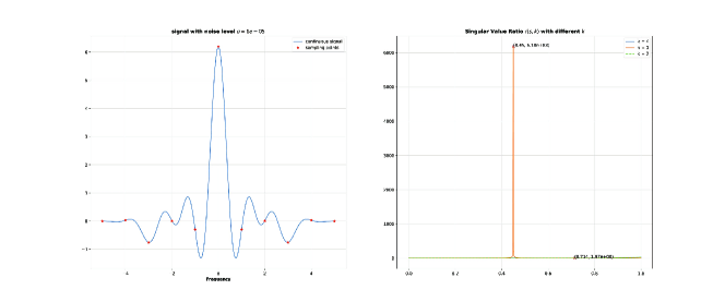
Figure 2.1: Left: The continuous Fourier data with ten sampled points. The variance is set as $v=0.455$ with 3 components whose means are $(0.3\pi,\pi,1.6\pi)$. Right: The singular value ratio of the Fourier data in the left. The ratio functional with three components peaks at 0.455.

2.3 Estimation of Means and Weights

In this subsection, we assume that the variance of the mixture model (2.1) is estimated and aims to estimate the means and weights. To achieve this, we employ the Multiple Signal Classification (MUSIC) algorithm[35, 18, 19, 37], which is widely utilized for line spectral estimation. The implementation details of the MUSIC algorithm can be found in Appendix 6.6.

We first modulate the Fourier data (2.1) by $e^{\hat{v}\omega^{2}}$, where $\hat{v}$ is the variance obtained from Algorithm 1. Subsequently, we apply the MUSIC algorithm with the input data

$$\left(e^{\hat{v}\omega_{-K}^{2}}Y_{n}(\omega_{-K}),\cdots,e^{\hat{v}\omega_{K}^{2}}Y_{n}(\omega_{K})\right)$$

and component number $\hat{k}$ obtained by Algorithm 1 to estimate the means.

To estimate the weight parameter $\boldsymbol{\theta}=\left(\pi_{1},\pi_{2},\quad,\pi_{k}\right)^{\mathrm{T}}\in\mathbb{R}^{k}$, we apply the conventional least square estimator with convex constraints. Denote

$$\boldsymbol{\psi}_{K}(\mu;v)=\left[e^{-v\omega_{-K}^{2}}e^{\iota\mu\omega_{-K}},e^{-v\omega_{-K+1}^{2}}e^{\iota\mu\omega_{-K+1}},\cdots,e^{-v\omega_{K}^{2}}e^{\iota\mu\omega_{K}}\right],$$

$$\boldsymbol{y}:=\begin{bmatrix}Y_{n}(\omega_{-K})\\ Y_{n}(\omega_{-K+1})\\ \vdots\\ Y_{n}(\omega_{K})\end{bmatrix},\quad\boldsymbol{Z}:=\begin{bmatrix}\boldsymbol{\psi}_{K}(\mu_{1};v)\\ \boldsymbol{\psi}_{K}(\mu_{2};v)\\ \vdots\\ \boldsymbol{\psi}_{K}(\mu_{k};v)\end{bmatrix}^{\mathrm{T}},\quad\boldsymbol{w}:=\begin{bmatrix}W(\omega_{-K})\\ W(\omega_{-K+1})\\ \vdots\\ W(\omega_{K})\end{bmatrix}.$$ (2.10)

Then equation (2.1) can be rewritten in the matrix form

$$\boldsymbol{y}=\boldsymbol{Z}\boldsymbol{\theta}+\boldsymbol{w}.$$ (2.11)

Therefore, if we denote

$$\hat{\boldsymbol{Z}}:=\begin{bmatrix}\boldsymbol{\psi}_{K}^{\mathrm{T}}(\hat{\mu}_{1};\hat{v})&\boldsymbol{\psi}_{K}^{\mathrm{T}}(\hat{\mu}_{2};\hat{v})&\cdots&\boldsymbol{\psi}_{K}^{\mathrm{T}}(\hat{\mu}_{\hat{k}};\hat{v})\end{bmatrix},$$ (2.12)

then the weights can be estimated by solving the following convex program:

$$\underset{\boldsymbol{\theta}=(\pi_{1},\cdots,\pi_{\hat{k}})^{\mathrm{T}}\in\mathbb{R}^{\hat{k}}}{\operatorname{minimize}} \left\lVert\boldsymbol{y}-\hat{\boldsymbol{Z}}\boldsymbol{\theta}\right\rVert_{2}$$ (2.13)

$$\operatorname{subject\ to} \sum_{j=1}^{\hat{k}}\pi_{j}=1,\pi_{j}\geq 0,j=1,\cdots,\hat{k}.$$ (2.14)

The parameter estimation algorithm can therefore be summarized as below.

Input: samples $X_{1},\cdots,X_{n}$, cutoff frequency $\Omega$, $K$, variance grid $\{v_{i}\}_{i=1}^{m}$, thresholding term $T$ (default $0$), model order $k$ (optional).

1

2Let $\hat{v},\hat{k},(\omega_{q},Y_{q})$ be the outputs of Algorithm 2 with all inputs above ;

3

4Let $(\hat{\mu}_{1},\cdots,\hat{\mu}_{\hat{k}})$ be the outputs of MUSIC with inputs $(e^{\hat{v}\omega_{-K}^{2}}Y_{-K},\cdots,e^{\hat{v}\omega_{K}^{2}}Y_{K})$ and $\hat{k}$ ;

5

6Let $\boldsymbol{y}=\begin{bmatrix}{Y}_{-K}&{Y}_{-K+1}&\cdots&{Y}_{K}\end{bmatrix}^{\mathrm{T}},\quad\boldsymbol{Z}=\begin{bmatrix}\boldsymbol{\psi}_{K}^{\mathrm{T}}(\hat{\mu}_{1};\hat{v})&\boldsymbol{\psi}_{K}^{\mathrm{T}}(\hat{\mu}_{2};\hat{v})&\cdots&\boldsymbol{\psi}_{K}^{\mathrm{T}}(\hat{\mu}_{\hat{k}};\hat{v})\end{bmatrix}$;

7 Let $(\hat{\pi}_{1},\cdots,\hat{\pi}_{\hat{k}})$ be the outcome of the optimization problem (2.13)-(2.14) ;

Output: variance $\hat{v}$, number of component $\hat{k}$, means $(\hat{\mu}_{1},\cdots,\hat{\mu}_{\hat{k}})$, weights $(\hat{\pi}_{1},\cdots,\hat{\pi}_{\hat{k}})$.

Algorithm 3 Parameter Estimation Algorithm of GMM

2.4 The Computation Resolution Limit for resolving the model order

In this subsection, we reveal that there exists a fundamental limit to the resolvability of the model order or the component number in the estimating of Gaussian mixture models due to the finite sample size. This resolvability depends crucially on the separation distance of the means of the Gaussian components and the sample size.

We recall the recent works [21, 20, 22] which are concerned with the line spectral estimation problem (6.12) of estimating a collection of point sources (or spectra) from their band-limited Fourier data with the presence of noise and the related problems. It is shown that to ensure an accurate estimation of the number of point sources with the presence of noise in the data, the minimum separation distance of the point sources needs to be greater than a certain threshold number, which is termed the computational resolution limit for the number detection problem. Moreover, up to a universal constant, this limit is characterized by the following formula

$$\mathcal{O}\left(\frac{1}{\Omega}\left(\frac{1}{SNR}\right)^{\frac{1}{2k-2}}\right),$$ (2.15)

where $\Omega$ is the frequency band, $SNR$ is the signal-to-noise ratio, and $k$ is the number of point sources. Similar conclusions were also derived for the support estimation problem.

Back to the mixture model (2.1), assuming that the variance is known and that the cut-off frequency is given by $\Omega$, then the means can be estimated from the following modulated data

$$\left(e^{{v}\omega_{-K}^{2}}Y(\omega_{-K}),\cdots,e^{{v}\omega_{K}^{2}}Y(\omega_{K})\right).$$

This becomes exactly the line spectra estimation problem. Note that the SNR is given by

$$\pi_{\min}e^{-\frac{v}{2}\Omega^{2}}/\|W\|_{\infty}$$

due to the amplification of noise by the modulation. Equation (2.15) then implies that to ensure an accurate estimation of the number of Gaussian components, the minimum separation distance between the means should be greater than a certain threshold number, which up to some universal constant is of the following form

$$\mathcal{O}\left(\frac{1}{\Omega}\left(\frac{\left\lVert W\right\rVert_{\infty}e^{\frac{v}{2}\Omega^{2}}}{\pi_{\min}}\right)^{\frac{1}{2k-2}}\right).$$ (2.16)

By choosing a proper cutoff frequency $\Omega$, we can minimize the threshold number (2.16). A straightforward calculation suggests that when $k\geq 2$ the optimal $\Omega$ is given by

$$\Omega_{\text{num}}=\sqrt{\frac{2k-2}{v}}.$$ (2.17)

The associated threshold number for the minimum separation of the means now becomes

$$\mathcal{O}\left(\sqrt{\frac{v}{2k-2}}\left(\frac{\|W\|_{\infty}}{\pi_{\min}}\right)^{\frac{1}{2k-2}}\right).$$ (2.18)

Note that in the model (2.1), $W(\cdot)$’s are Gaussian random variables with variances of the order $\mathcal{O}(\frac{1}{\sqrt{n}})$. The infinity norm $\|W\|_{\infty}$ may not be bounded. However, with high probability, we have

$$\|W\|_{\infty}=\mathcal{O}(\frac{1}{\sqrt{n}}).$$

Therefore, we can conclude that, in the case where the variance is available, to ensure an accurate estimation of the model order of the mixture model (1.2) with high probability, it is necessary that the minimum separation distance of the means should be greater than a threshold number of the following form

$$\mathcal{O}\left(\sqrt{\frac{v}{2k-2}}\left(\frac{1}{\pi_{\min}\sqrt{n}}\right)^{\frac{1}{2k-2}}\right).$$ (2.19)

In the case when the variance is not available and needs to be estimated, the estimation error may reduce the SNR for the line spectra estimation step, and hence the threshold number of the minimum separation distance of the means should be greater than the one given in (2.19). This will be evident from the numerical experiment in section 4. Nevertheless, formula (2.19) provides a lower bound on this threshold number. Following [21, 20, 22], we term this threshold number as the computational resolution limit for the model order estimation problem for the mixture model (2.1). It is important to obtain a sharper lower bound for this limit and we leave it for future work.

Finally, we note that in practice, the oracle cutoff frequency may not be available. We can alternatively set the cutoff frequency by ensuring that the modulus of the Fourier data is above the noise level. Suppose $n$ samples are generated from the mixture, then the noise level is of the order $\mathcal{O}(\frac{1}{\sqrt{n}})$ by the central limit theorem. Therefore, we can determine the cutoff frequency as the maximum $\Omega$ satisfying

$$\sup_{\omega\in[\Omega,+\infty)}\left\lvert Y(\omega)\right\rvert<\frac{1}{\sqrt{n}},$$

A binary search algorithm for choosing the cutoff frequency is given below:

Input: samples $X_{1},X_{2},\cdots,X_{n}$, search time $t$, initial guess of cutoff frequency $\Omega_{\max}$.

1 Initialize $\Omega_{\min}=0$;

2 for $i=1,\cdots,t$ do

3       Let $\Omega_{\text{mid}}=\frac{\Omega_{\min}+\Omega_{\max}}{2}$ and $M=\left\lvert\frac{1}{n}\sum_{j=1}^{n}e^{\iota\Omega_{\text{mid}}X_{j}}\right\rvert$;

4       if $M<\frac{1}{\sqrt{n}}$ then

5             Let $\Omega_{\max}=\Omega_{\text{mid}}$;

6       else

7            Let $\Omega_{\min}=\Omega_{\text{mid}}$;

8       end if

9      

10 end for

Output: cutoff frequency $\Omega_{\max}$.

Algorithm 4 Binary search of cutoff frequency

2.5 Computational Complexity

In this subsection, we analyze the computational complexity of Algorithm 1.

We use a fine grid of stepsize $\Delta v$ for identifying the variance parameter within the interval $[0,V]$. Given $2K+1$ Fourier data, a $(K+1)\times(K+1)$ Hankel matrix is constructed in Algorithm 1 for each $v$ on the grid. For each Hankel matrix, the time complexity of computing all its singular values is $O(K^{3})$. For each variance candidate on the grid, the complexity of computing the ratios is ${O}(K)$. Finding the maximum of all ratios is of complexity $O(\frac{V}{\Delta v}K)$. Therefore, the computational complexity of the Algorithm 1 is

$$\frac{V}{\Delta v}\cdot[O(K^{3})+O(K)]+O(\frac{V}{\Delta v}K)\sim{O}(\frac{V}{\Delta v}K^{3}).$$ (2.20)

In practice, we only require $K\geq k$. Therefore, $K={O}(k)$, and the computational complexity of the Algorithm 1 is

$${O}\left(\frac{V}{\Delta v}k^{3}\right).$$

We note that the computation complexity can be further reduced by using certain adaptive strategies to reduce the number of grid points for the variance search step.

3 Comparison with the EM Algorithm

In this section, we conduct several experiments to compare the efficiency of Algorithm 3 and the EM algorithm (see Appendix 6.7). To compare the performance of the two algorithms, we plot out the relative error of variance and the 1-Wasserstein distance error of mixing distribution defined as

$$W_{1}(\nu,\tilde{\nu})=\int\left\lvert F_{\nu}(t)-F_{\hat{\nu}}(t)\right\rvert\operatorname*{d}t$$

where $\hat{\nu}=\sum_{i=1}^{\hat{k}}\hat{\pi}_{i}\delta_{\hat{\mu}_{i}}$ is the estimated mixing distribution and $F_{\nu},F_{\hat{\nu}}$ denote the cumulative distribution function (CDF) of discrete measures $\nu,\hat{\nu}$. The average running time of each trial is included to compare the computational cost.

In the first experiment, we consider the following 2-component Gaussian mixtures

$$X_{i}\sim\frac{1}{2}\mathcal{N}(\mu_{1},\sigma^{2})+\frac{1}{2}\mathcal{N}(\mu_{2},\sigma^{2})$$ (3.1)

with $\mu_{1}=-0.5,\mu_{2}=0.5,\sigma^{2}=1$. For the EM algorithm, we randomly select two samples as the initial guess of means and set $\hat{\sigma}$ equal to the standard deviation of samples. The algorithm terminates when the log-likelihood increases less than $1\times 10^{-5}$ or it iterates for $1,000$ times. For Algorithm 3, we assume that the model order $k=2$ is known, and choose the cutoff frequency by Algorithm 4 with input $t=8,\tau=8.0$ and $\Omega=10.0$. A gird from $0$ to $2$ with grid size $1\times 10^{-2}$ is used and $T,K,k$ is set to be $0,4,2$, respectively.

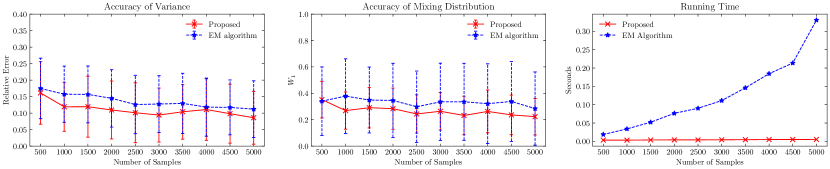
Figure 3.1: Comparison with the EM algorithm when the model order is known. For each sample size, we conducted 100 trials. The left plot shows the accuracy for variance estimation; The middle one shows the accuracy of the mixing distribution; The right one shows the average running time of each trial.

For each sample size, 100 trials are conducted and the results are shown in Figure 3.1. Our algorithm performs better than the EM algorithm in accuracy in all cases. Furthermore, our algorithm is significantly faster than the EM algorithm, especially for large sample sizes. This is because the EM algorithm accesses all the samples at each iteration but ours only uses them for computing the Fourier data $Y_{q}$ in the first step of Algorithm 2.

We next consider the extreme case in the 2-component mixture model with overlapping components. The samples are drawn from $\mathcal{N}(0,1)$. The setting of Algorithm 3 is the same as in the first experiment above except that the thresholding term is set as $T=\frac{20}{\sqrt{n}}$. The setup of the EM algorithm remains unchanged. 100 trials are conducted and we plot out the results in Figure 3.2. Although the model order is unknown to Algorithm 3 a prior, it achieves more accurate results than the EM algorithm.

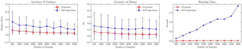
Figure 3.2: Comparison with EM algorithm for overlapping components. For each sample size, we conducted 100 trials. The left plot shows the accuracy for variance estimation; The middle one shows the accuracy of the mean estimation; The right one shows the average running time of each trial.

We also consider the case of a Gaussian mixture with 5 components and a unit variance. We generate the samples with the mixing distribution $\nu=0.2\delta_{-4}+0.2\delta_{-2}+0.2\delta_{0}+0.2\delta_{2}+0.2\delta_{4}$. For Algorithm 3, we set $K=5$ and keep other inputs unchanged as in the first experiment. For the EM algorithm, we set the termination criterion as either the log-likelihood increment is less than $1\times 10^{-6}$ or the iteration reaches $5,000$ times. The density function of the model and numerical results are shown in Figure 3.3. Again, our algorithm has demonstrated preferable performance in accuracy and running time, especially when the sample size is large.

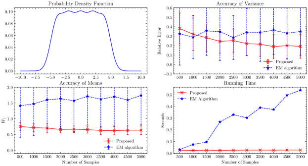
Figure 3.3: Comparison with EM algorithm (5 components). For each sample size, we conduct 100 trials. The upper left plot shows the probability density function of the distribution. The upper right one shows the accuracy for variance estimation; The lower left one shows the accuracy of the mixing distribution estimation; The lower right one shows the average running time of each trial.

Finally, we compare our algorithm with the EM algorithm in cases with a variety of separation distances between the means. For this purpose, we consider the following 2-component Gaussian mixture model

$$\frac{1}{2}\mathcal{N}(-\mu,1.0)+\frac{1}{2}\mathcal{N}(\mu,1.0),$$ (3.2)

where the separation distance between the means is $2\mu$. We compare Algorithm 3 and the EM algorithm. We draw $5,000$ samples for each $\mu$ and perform 100 trials. For Algorithm 3, the cutoff frequency is computed by Algorithm 4 with input $t=8,\Omega=10$, $K=2,T=0$, and the variance grid is set from $0$ to $2$ with grid size $1\times 10^{-2}$. The EM algorithm terminates if the log-likelihood function increases less than $1\times 10^{-5}$ or it iterates $1,000$ times. We use both one-component and two-component EM algorithms to estimate the parameters. Note that the one-component EM degenerates to the maximum likelihood estimator of Gaussian samples.

Figure 3.4: Comparison with the EM algorithm for different separation distances. For each different separation distance, we conducted $100$ trials. The upper left plot shows the accuracy of the variance estimation, the region that Algorithm 3 is less accurate than the EM falls in the overlapping region in Figure 4.1; The upper right plot shows the accuracy of the mixing distribution; The lower left one shows the average running time of each trial; The lower right one shows the average log-likelihood of each estimated model.

We plot out the results in Figure 3.4. The numerical result shows that the error of the two-component EM algorithm and ours is comparable when the two components are separated by less than 0.8, and our algorithm has better performance when the separation distance is larger than $1.4$. This can be explained by the computational resolution limit for the component number detection problem introduced in section 2.4. Due to the finite sample size, there exists a phase transition region between successful and unsuccessful number detection trials when the separation distance between the two components is between 0.8 and 1.4. Specifically, when the separation distance is below $1.4$, Algorithm 3 may return one or two as the component number case by case. The incorrect component number results in a larger estimation error for the variance.

We plot out the results of average log-likelihood in Table 3.1. It is clear that the log-likelihood from the one-component EM algorithm and two-component are extremely close when two components are separated by less than 0.8, which is again a consequence of the computation resolution limit. We also note that Algorithm 3 achieves log-likelihood values that are comparable to two-component EM’s, with even larger values when the separation distance is greater than 1.6.

$\mu$	0.4	0.6	0.8	1.0	1.2	1.4	1.6	1.8	2.0
EM	-7199.71	-7306.72	-7464.94	-7652.61	-7857.30	-8087.91	-8312.44	-8556.80	-8775.38
MLE	-7200.21	-7307.24	-7465.81	-7654.25	-7860.24	-8094.34	-8325.74	-8583.22	-8822.19
Proposed	-7202.46	-7309.52	-7468.70	-7655.97	-7860.30	-8089.28	-8311.45	-8554.25	-8772.35

Table 3.1: Average log-likelihood of different algorithms. The maximal log-likelihood is highlighted in bold. When the separation distance is large i.e. $\mu>1.6$, Algorithm 3 returns higher likelihood. When $\mu<1.6$, the EM algorithm returns a higher likelihood.

We point out that Algorithm 3 requires no initial guess and even the model order. This is different from the EM algorithm which requires both the model order and a good initial guess. It is known that the EM algorithm is sensitive to the initial guess, as a suboptimal initial guess can lead to the likelihood function being trapped in local minima, resulting in inaccurate estimations. In addition, our algorithm only uses the samples at the first step in computing the Fourier data. In contrast, the EM algorithm processes all the samples in each iteration. As a result, our algorithm has lower computational complexity.

4 Phase Transition in the model order estimation problem

In this section, we consider the model selection problem in the Gaussian mixture model (1.2). We demonstrate that there exists a phase transition phenomenon in the model order estimation problem which depends crucially on the minimum separation distance between the means and the sample size.

4.1 Phase transition

In this subsection, we illustrate the phase transition in the estimation of the model order i.e. the number of Gaussian components in the mixture models.

To avoid taking huge sizes of samples, we use the following Fourier data

$$Y^{\sigma}(\omega_{q})=e^{-v\omega_{q}^{2}}\sum_{i=1}^{k}\pi_{i}e^{\iota\mu_{i}\omega_{q}}+W(\omega_{q}),\quad-K\leq q\leq K,$$

where $W(\omega_{q})$ is generated randomly from the distribution $\mathcal{N}(0,\sigma^{2})+\iota\mathcal{N}(0,\sigma^{2})$. Here $\sigma$ is regarded as the noise level that is related to the sample number by $\sigma=\mathcal{O}(\frac{1}{\sqrt{n}})$. We conduct numerical experiments using Algorithm 1. We consider $k$ components of weight $\pi_{i}=\frac{1}{k}$ with a unit variance. In Algorithm 1, we set the size of the Hankel matrix to be $(k+1)\times(k+1)$ and the cutoff frequency $\Omega$ using (2.17).

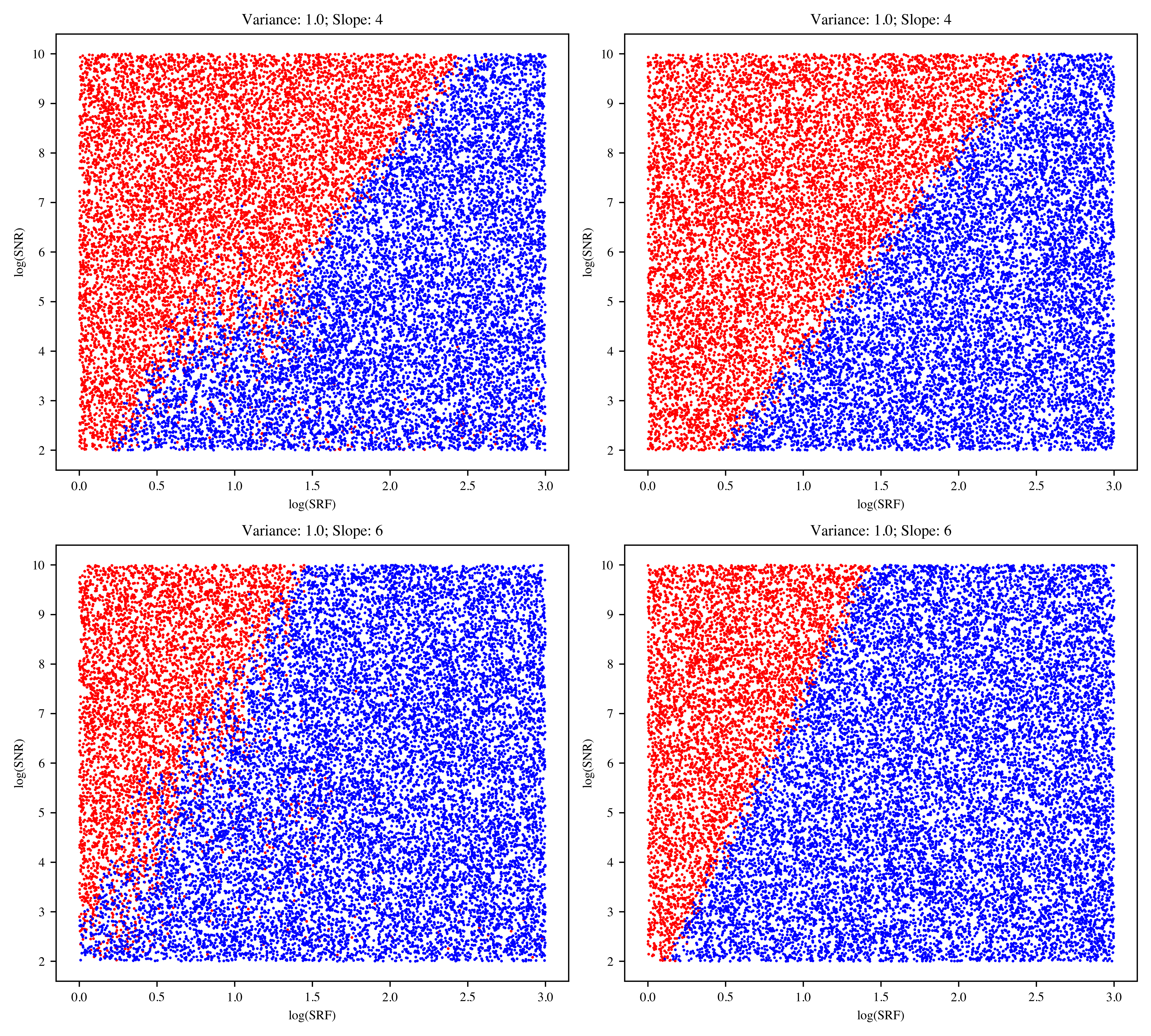
Figure 4.1: Phase transition in the model order estimating problem. $20,000$ trials are conducted for $k=2$ in the upper two plots and $k=3$ in the lower two plots. The phase transition region is sharper if the true variance is provided (left two plots). The slope of the phase transition line is approximately $2k$.

Following [21, 20, 22], we define for each trial a super-resolution factor $SRF=\frac{\pi}{d_{\min}\Omega}$ and the signal-to-noise ratio $SNR=\frac{\pi_{\min}}{\sigma}$. We take $20,000$ uniform samples in the square region $[0,3]\times[2,10]$ in the $\log(SRF)-\log(SNR)$ plane. For each sample, we generate a trial with the associated $SRF$ and $SNR$. We apply Algorithm 1 to each trial to estimate its component number. The results are shown in Figure 4.1. The successful trials are denoted by red points and the failed ones are blue ones. In the left two plots, the variances are unknown, and in the right two, the variance is known. We see clearly that there exists a phase transition phenomenon in the estimation problem. This phase transition can be explained by the computational resolution limit for the model order estimation problem introduced in the section 2.4. Due to the limited number of i.i.d samples from the mixture model, or the corruption of noise of the Fourier data, the minimum separation distance of the Gaussian means needs to be greater than a threshold number to guarantee an accurate estimation of the model order. We note that when the variance is given a prior, the transition region is sharper, as is seen in the right two plots, where the successful trials and unsuccessful ones are almost separated by a line of line of slope $2k$. We also note that some scattered outliers are away from the transition line. This is because the phase transition should be interpreted in the probability sense, as is explained in section 2.4.

4.2 The model order estimation problem

In this subsection, we address the model order estimation problem from the perspective of information criteria[2, 1, 17]. We consider the mixture model (3.2) with $\mu=0.5$ and draw i.i.d samples from it. The separation distance between the two means is $1$. We assume that the model order $k=2$ is unknown and want to estimate all the parameters including it. We set $K=2$ for Algorithm 3, which implies that the model may be interpreted as one-component or two-component mixtures. We shall compare its results with the one from the two-component EM algorithm.

Since the model orders are not assumed to be known, it makes no sense to compare the estimation accuracy of the parameters. Instead, we compare the log-likelihood of the estimated model from different algorithms and evaluate the model by the information criteria AIC and BIC. The formal AIC and BIC of a given model $\mathcal{M}$ is defined as

$$AIC_{\mathcal{M}} =2p-2\hat{ll}_{\mathcal{M}},$$

$$BIC_{\mathcal{M}} =p\ln{(n)}-2\hat{ll}_{\mathcal{M}},$$

where $p$ is the number of the free parameters in the model $\mathcal{M}$, $n$ is the number of the samples, and $\hat{ll}_{\mathcal{M}}$ is the maximized value of the log-likelihood function of the model $\mathcal{M}$. In our setting, we replace $\hat{ll}_{\mathcal{M}}$ by the value of log-likelihood of the estimated model $\mathcal{M}$. We plot out the difference of the log-likelihood (the higher the better) as well as each information criterion (the lower the better) defined as

$$\Delta ll=ll_{\mathcal{M}_{EM}}-ll_{\mathcal{\hat{M}}},\quad\Delta AIC=AIC_{\mathcal{M}_{EM}}-AIC_{\mathcal{\hat{M}}},\quad\Delta BIC=BIC_{\mathcal{M}_{EM}}-BIC_{\mathcal{\hat{M}}},$$

where $\hat{\mathcal{M}},\mathcal{M}_{EM}$ are the models estimated by Algorithm 3 and the EM algorithm. The numerical results are shown in the upper left plot of Figure 4.2. Algorithm 3 achieves better likelihood, BIC, and AIC scores than the EM algorithm when the sample size is larger than $3,000$.

Similarly, we compare the results obtained from the one-component, the two-component, and the three-component EM algorithm. The results are shown in Figure 4.2. The one-component algorithm achieves better likelihood, AIC, and BIC scores, even though the model order is not correct. We remark that this is a consequence of the computational resolution limit for the model order estimation problem since the separation distance $1$ is below this limit. We also note that as the sample number increases, our algorithm can yield the correct model order with high probability as is shown in Remark 2.2. However, criteria based on likelihood and AIC or BIC cannot provide a guarantee for this.

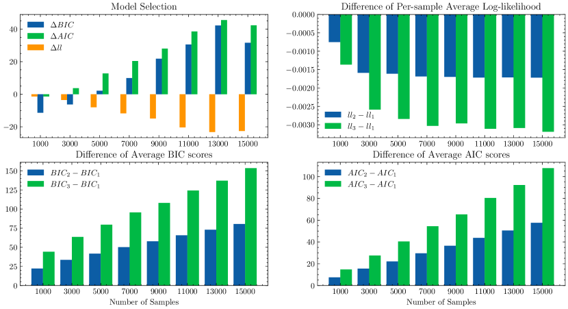
Figure 4.2: The upper left plot shows the difference in the log-likelihood, AIC, and BIC of the 2-component EM algorithm with Algorithm 3. Algorithm 3 achieves better likelihood in each sample size. The AIC and BIC scores of Algorithm 3 are better when the sample size increases. The other three plots show the difference in log-likelihood, BIC, and AIC of the EM algorithm with different component numbers, respectively. The blue bars represent the difference between the two-component EM and the one-component one. The green bars represent the differences between the three-component EM and the one-component one. For each sample size, the one-component achieves the better scores though the model order is incorrect.

5 Conclusion and Future Works

In this paper, we propose a novel method for estimating the parameters in one-dimensional Gaussian mixture models with unified variance by taking advantage of the Hankel structure inherent in the Fourier data (the empirical characteristic function) obtained from i.i.d samples of the mixture. The method can estimate the variance and the model order simultaneously without prior information. We have proved the consistency of the method and demonstrated its efficiency in comparison with the EM algorithm. We further reveal that there exists a fundamental limit to the resolvability of the model order with finite sample size. We characterized this limit by the computation resolution limit. We demonstrate that there exists a phase transition phenomenon in the parameter estimation problem due to this fundamental limit. Moreover, we show that our proposed method can resolve the model order correctly with a sufficiently large sample size, which however is not the case for classic model order selection methods such as AIC or BIC. In the future, we plan to extend this method to higher dimensions and also to the case with multiple variances.

6 Appendix

6.1 Proof of Theorem 2.1

We first introduce two useful lemmas.

Lemma 6.1.

Let $\boldsymbol{D}$ be an $m\times n$ matrix, $\boldsymbol{A}=\mathrm{diag}(\pi_{1},\cdots,\pi_{n})$ be an $n\times n$ diagonal matrix. Let $1\leq j_{1}<j_{2}<\cdots<j_{m}\leq n$, and $\boldsymbol{D}_{j_{1}j_{2}\cdots j_{m}}$ be the $m\times m$ matrix consisting the $j_{1},j_{2},\cdots,j_{m}$-th columns of $\boldsymbol{D}$. Then

$$\det\left(\boldsymbol{D}\boldsymbol{A}\boldsymbol{D}^{\mathrm{T}}\right)=\sum_{1\leq j_{1}<j_{2}<\cdots<j_{m}\leq n}\left(\det\left(\boldsymbol{D}_{j_{1}j_{2}\cdots j_{m}}\right)\right)^{2}\prod_{i=1}^{m}\pi_{j_{i}}.$$

Proof.

Denote $\boldsymbol{d}_{i}$ as the $i$-th column of $\boldsymbol{D}$. Then

$$\det\left(\boldsymbol{D}\boldsymbol{A}\boldsymbol{D}^{\mathrm{T}}\right) =\det\left(\begin{bmatrix}\boldsymbol{d}_{1},\boldsymbol{d}_{2},\cdots,\boldsymbol{d}_{n}\end{bmatrix}\boldsymbol{A}\begin{bmatrix}\boldsymbol{d}_{1},\boldsymbol{d}_{2},\cdots,\boldsymbol{d}_{n}\end{bmatrix}^{\mathrm{T}}\right)$$

$$=\det\left(\begin{bmatrix}\pi_{1}\boldsymbol{d}_{1},\pi_{2}\boldsymbol{d}_{2},\cdots,\pi_{n}\boldsymbol{d}_{n}\end{bmatrix}\begin{bmatrix}\boldsymbol{d}_{1},\boldsymbol{d}_{2},\cdots,\boldsymbol{d}_{n}\end{bmatrix}^{\mathrm{T}}\right).$$

Using the Cauchy-Binet formula, we further obtain

$$\det\left(\boldsymbol{D}\boldsymbol{A}\boldsymbol{D}^{\mathrm{T}}\right) =\sum_{1\leq j_{1}<j_{2}<\cdots<j_{m}\leq n}\det\left(\begin{bmatrix}a_{j_{1}}\boldsymbol{d}_{j_{1}},\cdots,a_{j_{m}}\boldsymbol{d}_{j_{m}}\end{bmatrix}\begin{bmatrix}\boldsymbol{d}_{j_{1}},\cdots,\boldsymbol{d}_{j_{m}}\end{bmatrix}^{\mathrm{T}}\right)$$

$$=\sum_{1\leq j_{1}<j_{2}<\cdots<j_{m}\leq n}\det\left(\begin{bmatrix}\boldsymbol{d}_{j_{1}},\cdots,\boldsymbol{d}_{j_{m}}\end{bmatrix}\begin{bmatrix}\boldsymbol{d}_{j_{1}},\cdots,\boldsymbol{d}_{j_{m}}\end{bmatrix}^{\mathrm{T}}\right)\prod_{i=1}^{m}a_{j_{i}}$$

$$=\sum_{1\leq j_{1}<j_{2}<\cdots<j_{m}\leq n}\left(\det\left(\boldsymbol{d}_{j_{1}j_{2}\cdots j_{m}}\right)\right)^{2}\prod_{i=1}^{m}a_{j_{i}}.$$

∎

For a vector $\boldsymbol{y}=\left[y_{-K},y_{-K+1},\cdots,y_{K}\right]\in\mathbb{C}^{2K+1}$, denote

$$\text{Hankel}(\boldsymbol{y})=\begin{bmatrix}y_{-K}&y_{-K+1}&\cdots&y_{0}\\ y_{-K+1}&y_{-K+2}&\cdots&y_{1}\\ \vdots&\vdots&\ddots&\vdots\\ y_{0}&y_{1}&\cdots&y_{K}\end{bmatrix}\in\mathbb{C}^{(K+1)\times(K+1)}$$

as the square Hankel matrix formed by $\boldsymbol{y}$.

Lemma 6.2.

Let $K=k$, then $\mathrm{rank}\left(\boldsymbol{E}(u)\circ\boldsymbol{Y}\right)=k+1$ for $u$ sufficiently close to but not equal to $v$.

Proof.

Notice that $\boldsymbol{E}(u)\circ\boldsymbol{Y}=\boldsymbol{E}(u-v)\circ\boldsymbol{H}$ and denote

$$\boldsymbol{H}(s)=\boldsymbol{E}(s)\circ\boldsymbol{H}=\text{Hankel}(\boldsymbol{\alpha})$$

where

$$\boldsymbol{\alpha}=(\alpha_{q})_{-K\leq q\leq K},\quad\alpha_{q}=e^{-s\omega_{q}^{2}}\sum_{i=1}^{k}\pi_{i}e^{\iota\mu_{i}\omega_{q}}.$$

We only need to prove that rank $\left(\boldsymbol{H}(s)\right)=k+1$ for $s$ sufficiently small but not $0$. Indeed, for $|s|\ll 1$, we have

$$e^{-s\omega_{q}^{2}}=1-s\omega_{q}^{2}+\mathcal{O}(s^{2}).$$

It follows that

$$\alpha_{q}=\beta_{q}+\mathcal{O}(s^{2}),\quad\beta_{q}=(1-s\omega_{q}^{2})\sum_{i=1}^{k}\pi_{i}e^{\iota\mu_{i}\omega_{q}},\quad\text{for }-K\leq q\leq K.$$

Let $\boldsymbol{\beta}=(\beta_{q})_{-K\leq q\leq K}$. Then

$$\det\boldsymbol{H}(s)=\det\left(\text{Hankel}(\boldsymbol{\alpha})\right)=\det\left(\text{Hankel}(\boldsymbol{\beta})\right)+\mathcal{O}(s^{2}).$$ (6.1)

We shall prove that the determinant of $\boldsymbol{H}(s)$ has a nonzero first-order term. Observe that for $|\Delta\mu|\ll 1$,

$$\omega_{q}^{2}e^{\iota\mu_{i}\omega_{q}}=\frac{e^{\iota(\mu_{i}+\Delta\mu)\omega_{q}}+e^{\iota(\mu_{i}-\Delta\mu)\omega_{q}}-2e^{\iota\mu_{i}\omega_{q}}}{{\left(\Delta\mu\right)}^{2}}+\mathcal{O}(\Delta\mu).$$

We can rewrite

$$\beta_{q}=\gamma_{q}+\mathcal{O}(\Delta\mu),\quad-K\leq q\leq K$$

where

$$\gamma_{q}=\sum_{i=1}^{k}\left(\pi_{i}\left(1-\frac{2s}{\left(\Delta\mu\right)^{2}}\right)e^{\iota\mu_{i}\omega_{q}}+\pi_{i}\frac{s}{\left(\Delta\mu\right)^{2}}e^{\iota(\mu_{i}-\Delta\mu)\omega_{q}}+\pi_{i}\frac{s}{\left(\Delta\mu\right)^{2}}e^{\iota(\mu_{i}+\Delta\mu)\omega_{q}}\right).$$

By (6.1),

$$\det\boldsymbol{H}(s)=\det\left(\text{Hankel}(\boldsymbol{\beta})\right)+\mathcal{O}(s^{2})=\det\left(\text{Hankel}(\boldsymbol{\gamma})\right)+\mathcal{O}(s^{2})+\mathcal{O}(\Delta\mu)$$ (6.2)

where $\boldsymbol{\gamma}=(\gamma_{q})_{-K\leq q\leq K}$. Using the Vandermonde decomposition of the Hankel matrix, we have

$$\text{Hankel}(\boldsymbol{\gamma})=\boldsymbol{D}_{\Delta\mu}\left(\mu_{1},\cdots,\mu_{k}\right)\boldsymbol{\Pi}_{\Delta\mu,s}\boldsymbol{D}_{\Delta\mu}\left(\mu_{1},\cdots,\mu_{k}\right)^{\mathrm{T}}$$

where

$$\boldsymbol{D}_{\Delta\mu}\left(\mu_{1},\cdots,\mu_{k}\right)=\begin{bmatrix}\boldsymbol{\phi}(\mu_{1}-\Delta\mu),\boldsymbol{\phi}(\mu_{1}),\boldsymbol{\phi}(\mu_{1}+\Delta\mu),\cdots,\boldsymbol{\phi}(\mu_{k}-\Delta\mu),\boldsymbol{\phi}(\mu_{k}),\boldsymbol{\phi}(\mu_{k}+\Delta\mu)\end{bmatrix}\in\mathbb{C}^{(K+1)\times 3k},$$

$$\boldsymbol{\Pi}_{\Delta\mu,s}=\text{diag}\Biggl{\{} \pi_{1}e^{-\iota\Omega(\mu_{1}-\Delta\mu)}\frac{s}{(\Delta\mu)^{2}},\pi_{1}e^{-\iota\Omega\mu_{1}}\left(1-\frac{2s}{(\Delta\mu)^{2}}\right),\pi_{1}e^{-\iota\Omega(\mu_{1}+\Delta\mu)}\frac{s}{(\Delta\mu)^{2}},\cdots,$$

$$\pi_{k}e^{-\iota\Omega(\mu_{1}-\Delta\mu)}\frac{s}{(\Delta\mu)^{2}},\pi_{k}e^{-\iota\Omega\mu_{k}}\left(1-\frac{2s}{(\Delta\mu)^{2}}\right),\pi_{k}e^{-\iota\Omega(\mu_{k}+\Delta\mu)}\frac{s}{(\Delta\mu)^{2}}\Biggl{\}}\in\mathbb{C}^{3k\times 3k}.$$

Then Lemma 6.1 implies

$$\det\left(\text{Hankel}(\boldsymbol{\gamma})\right) =\det\left(\boldsymbol{D}_{\Delta\mu}\left(\mu_{1},\cdots,\mu_{k}\right)\boldsymbol{\Pi}_{\Delta\mu,s}\boldsymbol{D}_{\Delta\mu}\left(\mu_{1},\cdots,\mu_{k}\right)^{\mathrm{T}}\right)$$ (6.3)

$$=s\left(\prod_{i=1}^{k}\pi_{i}e^{-\iota\Omega\mu_{i}}\right)\left(\sum_{i=1}^{k}\frac{D_{i,-}^{2}+D_{i,+}^{2}}{(\Delta\mu)^{2}}\pi_{i}e^{-\iota\Omega\mu_{i}}\right)$$ (6.4)

where

$$D_{i,-}=\det\left\{\begin{bmatrix}\boldsymbol{\phi}(\mu_{1}),\boldsymbol{\phi}(\mu_{2}),\cdots,\boldsymbol{\phi}(\mu_{i}-\Delta\mu),\boldsymbol{\phi}(\mu_{i}),\cdots,\boldsymbol{\phi}(\mu_{k})\end{bmatrix}\right\},$$

$$D_{i,+}=\det\left\{\begin{bmatrix}\boldsymbol{\phi}(\mu_{1}),\boldsymbol{\phi}(\mu_{2}),\cdots,\boldsymbol{\phi}(\mu_{i}),\boldsymbol{\phi}(\mu_{i}+\Delta\mu),\cdots,\boldsymbol{\phi}(\mu_{k})\end{bmatrix}\right\}.$$

Using the formula for the determinant of the Vandermonde matrix, we have

$$D_{i,-} =(-1)^{i+1}\prod_{1\leq j<l\leq k}\left(e^{\iota\mu_{l}h}-e^{\iota\mu_{j}h}\right)\prod_{j=1}^{k}\left(e^{\iota\mu_{j}h}-e^{\iota(\mu_{i}-\Delta\mu)h}\right)$$

$$=(-1)^{i+1}\prod_{1\leq j<l\leq k}\left(e^{\iota\mu_{l}h}-e^{\iota\mu_{j}h}\right)\prod_{j\neq i}\left(e^{\iota\mu_{j}h}-e^{\iota\mu_{i}h}\right)ihe^{\iota\mu_{i}h}\Delta\mu+\mathcal{O}((\Delta\mu)^{2})$$

and

$$D_{i,+}=(-1)^{i+1}\prod_{1\leq j<l\leq k}\left(e^{\iota\mu_{l}h}-e^{\iota\mu_{j}h}\right)\prod_{j\neq i}\left(e^{\iota\mu_{j}h}-e^{\iota\mu_{i}h}\right)ihe^{\iota\mu_{i}h}\Delta\mu+\mathcal{O}((\Delta\mu)^{2}).$$

Substituting the above two formulas into (6.1), we further obtain

$$\det\boldsymbol{H}(s) =\det\left(\text{Hankel}(\boldsymbol{\gamma})\right)+\mathcal{O}(s^{2})+\mathcal{O}(\Delta\mu)$$

$$=s\left(\prod_{i=1}^{k}\pi_{j}e^{-\iota\Omega\mu_{i}}\right)\left(\sum_{i=1}^{k}2\pi_{i}e^{-\iota\Omega\mu_{i}}e^{\iota 2\mu_{i}h}h^{2}\left(\prod_{1\leq j<l\leq k}\left(e^{\iota\mu_{l}h}-e^{\iota\mu_{j}h}\right)\prod_{j\neq i}\left(e^{\iota\mu_{j}h}-e^{\iota\mu_{i}h}\right)\right)^{2}\right)$$

$$\quad+\mathcal{O}(s\Delta\mu)+\mathcal{O}(s^{2})+\mathcal{O}(\Delta\mu)$$

$$=s\cdot 2h^{2}\left(\prod_{i=1}^{k}\pi_{i}\right)\left(\prod_{1\leq j<l\leq k}\left(e^{\iota\mu_{l}h}-e^{\iota\mu_{j}h}\right)\right)^{2}\left(\sum_{i=1}^{k}\pi_{i}e^{-\iota\Omega\mu_{j}}e^{2i\mu_{i}h}\left(\prod_{j\neq i}\left(e^{\iota\mu_{j}h}-e^{\iota\mu_{i}h}\right)\right)^{2}\right)$$

$$\quad+\mathcal{O}(s\Delta\mu)+\mathcal{O}(s^{2})+\mathcal{O}(\Delta\mu)$$

$$=s\cdot 2h^{2}\left(\prod_{i=1}^{k}\pi_{i}\right)\left(\prod_{1\leq j<l\leq k}\left(e^{\iota\mu_{l}h}-e^{\iota\mu_{j}h}\right)\right)^{2}\left(\sum_{i=1}^{k}\pi_{i}e^{\iota\mu_{i}h}\left(\prod_{j\neq i}\left(e^{\iota(\mu_{j}-\mu_{i})h}-1\right)\right)^{2}\right)$$

$$\quad+\mathcal{O}(s\Delta\mu)+\mathcal{O}(s^{2})+\mathcal{O}(\Delta\mu).$$

Let $\Delta\mu\rightarrow 0$, then for $s$ sufficiently small, we have

$$\det\boldsymbol{H}(s)=s\cdot 2h^{2}\left(\prod_{i=1}^{k}\pi_{i}\right)\left(\prod_{1\leq j<l\leq k}\left(e^{\iota\mu_{l}h}-e^{\iota\mu_{j}h}\right)\right)^{2}\left(\sum_{i=1}^{k}\pi_{i}e^{\iota\mu_{i}h}\left(\prod_{j\neq i}\left(e^{\iota(\mu_{j}-\mu_{i})h}-1\right)\right)^{2}\right)+\mathcal{O}(s^{2}).$$

Since $\prod_{1\leq j<l\leq k}\left(e^{\iota\mu_{l}h}-e^{\iota\mu_{j}h}\right)\neq 0$, and by assumption 2.5, we can conclude that $\det\boldsymbol{H}(s)$ has the nonzero first order term. Therefore $\boldsymbol{H}(s)$ is of full rank for $s$ sufficiently small but not $0$. ∎

Proof of Theorem 2.1 By the previous lemma, for $K=k$ we have $\text{rank}(\boldsymbol{H}(s))=k+1$ for $s$ sufficiently close to but not equal to $0$. On the other hand, $\text{rank}(\boldsymbol{H}(0))=k$. Therefore, $\sigma(s,k+1)=0$ if and only if $s=v$ for $s$ in a small neighborhood of $v$. It follows that $r(s,l)=\infty$ if and only if $s=v$ and $l=k$ for $s$ in a small neighborhood of $0$. This proves Theorem 2.1 for the case $K=k$.

We next consider the case when $K>k$. Note that $\boldsymbol{H}(s)$ has the following block matrix form:

$$\boldsymbol{H}(s)=\begin{bmatrix}\boldsymbol{H}_{k+1}(s)&*\\ *&*\end{bmatrix}$$

where

$$\boldsymbol{H}_{k+1}(s)=\begin{bmatrix}e^{-s\omega_{-K}^{2}}&\cdots&e^{-s\omega_{-K+k}^{2}}\\ \vdots&\ddots&\vdots\\ e^{-s\omega_{-K+k}^{2}}&\cdots&e^{-s\omega_{-K+2k}^{2}}\end{bmatrix}\circ\begin{bmatrix}\sum_{i=1}^{k}\pi_{i}e^{\iota\mu_{i}\omega_{-K}}&\cdots&\sum_{i=1}^{k}\pi_{i}e^{\iota\mu_{i}\omega_{-K+n}}\\ \vdots&\ddots&\vdots\\ \sum_{i=1}^{k}\pi_{i}e^{\iota\mu_{i}\omega_{-K+k}}&\cdots&\sum_{i=1}^{k}\pi_{i}e^{\iota\mu_{i}\omega_{-K+2k}}\end{bmatrix}.$$

By Lemma 6.2, rank$(\boldsymbol{H}_{k+1}(s))=k+1$ for $s$ sufficiently close to but not equal to $0$. Therefore $\boldsymbol{H}(s)$ has rank at least $k+1$, which completes the proof.

6.2 Proof of Proposition 2.1

Proof.

Recall that

$$Y_{n}(\omega)=\sum_{j=1}^{n}\frac{e^{\iota\omega X_{j}}}{n}$$

and note that $-\frac{1}{n}\leq\frac{e^{\iota\omega X_{j}}}{n}\leq\frac{1}{n}$. By Hoeffding’s inequality, for any $\epsilon>0$,

$$\mathbb{P}\left(|Y_{n}(\omega)-Y(\omega)|\geq{n^{-\frac{1}{2}-\epsilon}}\right) \leq 2\text{exp}\left(-\frac{1}{2}n^{-2\epsilon}\right).$$

Therefore

$$\mathbb{P}\left(\left\lVert W\right\rVert_{\infty}\geq n^{-\frac{1}{2}-\epsilon}\right) \leq\sum_{q=-K}^{K}\mathbb{P}\left(|Y_{n}(\omega_{q})-Y(\omega_{q})|\geq n^{-\frac{1}{2}-\epsilon}\right)$$

$$\leq 2\left(2K+1\right)\text{exp}\left(-\frac{1}{2}n^{-2\epsilon}\right).$$

∎

6.3 Proof of Theorem 2.2

The following results are needed to complete the proof.

Proposition 6.1.

(Wely’s Theorem[38]) Let $\boldsymbol{M}$ be a $m\times n$ matrix, and $\sigma_{l}(\boldsymbol{M})$ its $l$-th singular value. Let $\boldsymbol{\Delta}\in\mathbb{C}^{m\times n}$ be a perturbation to $\boldsymbol{M}$. Then the following bound holds for the perturbed singular values

$$|\sigma_{l}(\boldsymbol{M}+\boldsymbol{\Delta})-\sigma_{l}(\boldsymbol{M})|\leq||\boldsymbol{\Delta}||.$$

Lemma 6.3.

Let $\boldsymbol{A},\boldsymbol{B}\in\mathbb{C}^{m\times n}$, then

$$\|\boldsymbol{A}\circ\boldsymbol{B}\|\leq\sqrt{n}\sup_{\begin{subarray}{c}1\leq i\leq m\\ 1\leq j\leq n\end{subarray}}|\boldsymbol{A}_{ij}|\|\boldsymbol{B}\|.$$

Proof.

Denote $\boldsymbol{e}_{i}$ as the $i$-th standard basis of $\mathbb{C}^{n}$. For any vector $\boldsymbol{v}\in\mathbb{C}^{n}$, we have $\boldsymbol{v}=\sum_{i=1}^{n}v_{i}\boldsymbol{e}_{i}$. Then

$$\|\boldsymbol{A}\circ\boldsymbol{B}\boldsymbol{v}\| =\|\sum_{i=1}^{n}v_{i}(\boldsymbol{A}\circ\boldsymbol{B})\boldsymbol{e}_{i}\|\leq\sum_{i=1}^{n}|v_{i}|\|(\boldsymbol{A}\circ\boldsymbol{B})\boldsymbol{e}_{i}\|\leq\sum_{i=1}^{n}|v_{i}|\sup_{1\leq j\leq n}|\boldsymbol{A}_{ij}|\|\boldsymbol{B}\boldsymbol{e}_{i}\|$$

$$\leq\|\boldsymbol{v}\|_{1}\sup_{\begin{subarray}{c}1\leq i\leq m\\ 1\leq j\leq n\end{subarray}}|\boldsymbol{A}_{ij}|\|\boldsymbol{B}\|\leq\sqrt{n}\|\boldsymbol{v}\|_{2}\sup_{\begin{subarray}{c}1\leq i\leq m\\ 1\leq j\leq n\end{subarray}}|\boldsymbol{A}_{ij}|\|\boldsymbol{B}\|.$$

∎

Proposition 6.2.

(Theorem 1 in [10]). Let $x_{i}\neq x_{j}$ for $i\neq j$. Let

$$\boldsymbol{V}_{k}=\begin{bmatrix}1&1&\cdots&1\\ x_{1}&x_{2}&\cdots&x_{k}\\ \vdots&\vdots&\ddots&\vdots\\ x_{1}^{k-1}&x_{2}^{k-1}&\cdots&x_{k}^{k-1}\end{bmatrix}$$

be a Vandermonde matrix. Then

$$||\boldsymbol{V}_{k}^{-1}||_{\infty}\leq\max_{1\leq j\leq k}\prod_{i=1,i\neq j}^{k}\frac{1+|x_{i}|}{|x_{i}-x_{j}|}.$$ (6.5)

Lemma 6.4.

Let $s>k-1$, denote

$$\boldsymbol{V}_{k-1}(k)=\left[\boldsymbol{\phi}_{k-1}(e^{\iota\mu_{1}}),\boldsymbol{\phi}_{k-1}(e^{\iota\mu_{2}}),\cdots,\boldsymbol{\phi}_{k-1}(e^{\iota\mu_{k}})\right]\in\mathbb{C}^{k\times k}$$

$$\boldsymbol{V}_{s}(k)=\left[\boldsymbol{\phi}_{s}(e^{\iota\mu_{1}}),\boldsymbol{\phi}_{s}(e^{\iota\mu_{2}}),\cdots,\boldsymbol{\phi}_{s}(e^{\iota\mu_{k}})\right]\in\mathbb{C}^{(s+1)\times k}$$

Then

$$\sigma_{*}(\boldsymbol{V}_{s}(k))\geq\sigma_{*}(\boldsymbol{V}_{k-1}(k))\geq\frac{1}{\left\lVert\boldsymbol{V}_{k-1}(k)^{-1}\right\rVert}.$$

The proof of the lemma can be found in Proposition 4.4 in [22].

6.4 Proof of Theorem 2.2

Proof.

Denote $\sigma(v,l),\sigma^{\boldsymbol{W}}(v,l)$ as the $l$-th singular value of matrix $\boldsymbol{H}=\boldsymbol{E}(v)\circ\boldsymbol{Y}$ and $\boldsymbol{E}(v)\circ\boldsymbol{Y}^{\boldsymbol{W}}=\boldsymbol{E}(v)\circ\boldsymbol{Y}+\boldsymbol{E}(v)\circ\boldsymbol{W}$, respectively. Apply Wely’s Theorem (Proposition 6.1) on the $k$ th and $k+1$ th singular values, we have

$$|\sigma^{\boldsymbol{W}}(v,k)-\sigma(v,k)|\leq||\boldsymbol{E}(v)\circ\boldsymbol{W}||,$$

$$|\sigma^{\boldsymbol{W}}(v,k+1)-\sigma(v,k+1)|\leq||\boldsymbol{E}(v)\circ\boldsymbol{W}||.$$

Since the Hankel matrix $\boldsymbol{H}$ has rank at most $k$, it holds that $\sigma(v,k+1)=0$. Therefore

$$\frac{\sigma^{\boldsymbol{W}}(v,k)}{\sigma^{\boldsymbol{W}}(v,k+1)}\geq\frac{\sigma(v,k)-||\boldsymbol{E}(v)\circ\boldsymbol{W}||}{||\boldsymbol{E}(v)\circ\boldsymbol{W}||}=\frac{\sigma(v,k)}{||\boldsymbol{E}(v)\circ\boldsymbol{W}||}-1.$$ (6.6)

We now estimate $\sigma(v,k)$. Notice that $\boldsymbol{H}=\boldsymbol{D}\boldsymbol{\Pi}\boldsymbol{D}^{\mathrm{T}}$. Let $\ker(\boldsymbol{D}^{\mathrm{T}})$ be the kernel space of $\boldsymbol{D}^{\mathrm{T}}$ and $\ker^{\bot}(\boldsymbol{D}^{\mathrm{T}})$ be its orthogonal complement. We have

$$\sigma(v,k)=\sigma_{*}(\boldsymbol{D}\boldsymbol{\Pi}\boldsymbol{D}^{\mathrm{T}})=\min_{\begin{subarray}{c}\left\lVert\boldsymbol{x}\right\rVert_{2}=1\\ \boldsymbol{x}\in\ker^{\bot}(\boldsymbol{D}^{\mathrm{T}})\end{subarray}}\left\lVert\boldsymbol{D}\boldsymbol{\Pi}\boldsymbol{D}^{\mathrm{T}}\boldsymbol{x}\right\rVert\geq\sigma_{*}(\boldsymbol{D}\boldsymbol{\Pi})\sigma_{*}(\boldsymbol{D}^{\mathrm{T}})\geq\sigma_{*}(\boldsymbol{D})\sigma_{*}(\boldsymbol{\Pi})\sigma_{*}(\boldsymbol{D}).$$ (6.7)

Recall that $\boldsymbol{D}=\left[\boldsymbol{\phi}_{K}(e^{\iota\mu_{1}}),\boldsymbol{\phi}_{K}(e^{\iota\mu_{2}}),\cdots,\boldsymbol{\phi}_{K}(e^{\iota\mu_{k}})\right]$. Since $K>k-1$, using Lemma 6.4 and Proposition 6.2, we have

$$\sigma_{*}(\boldsymbol{D})=\sigma_{*}(\boldsymbol{V}_{K}(k)) \geq\sigma_{*}(\boldsymbol{V}_{k-1}(k))\geq\frac{1}{||\boldsymbol{V}_{k-1}^{-1}(k)||}\geq\frac{1}{\sqrt{k}||\boldsymbol{V}_{k-1}^{-1}(k)||_{\infty}}$$

$$\geq\frac{1}{\sqrt{k}}\min_{1\leq j\leq k}\prod_{i=1,i\neq j}^{k}\frac{|e^{\iota\mu_{i}}-e^{\iota\mu_{j}}|}{2}.$$

Note that for $\mu_{i},\mu_{j}\in[-\frac{\pi}{2h},\frac{\pi}{2h})$,

$$|e^{\iota\mu_{i}h}-e^{\iota\mu_{j}h}|\geq\frac{2h}{\pi}|\mu_{i}-\mu_{j}|.$$

It follows that

$$\prod_{i=1,i\neq j}^{k}\frac{|e^{\iota\mu_{i}h}-e^{\iota\mu_{j}h}|}{2} \geq(\frac{h}{\pi})^{k-1}\prod_{i=1,i\neq j}^{k}|\mu_{i}-\mu_{j}|\geq(\frac{h}{\pi})^{k-1}\prod_{i<j}^{k}|\mu_{i}-\mu_{j}|\prod_{i>j}^{k}|\mu_{i}-\mu_{j}|$$

$$\geq(\frac{h}{\pi})^{k-1}(j-1)!d_{\min}^{j-1}(k-j)!d_{\min}^{k-j}=(\frac{hd_{\min}}{\pi})^{k-1}(j-1)!(k-j)!.$$

Therefore,

$$\sigma_{*}(\boldsymbol{D})\geq\frac{\zeta(k)}{\sqrt{k}}(\frac{hd_{\min}}{\pi})^{k-1}$$

where $\zeta(k)=\max_{1\leq j\leq k}(j-1)!(k-j)!$. Then by (6.7),

$$\sigma(v,k) \geq\sigma_{*}(\boldsymbol{\Pi})\left(\frac{\zeta(k)}{\sqrt{k}}(\frac{hd_{\min}}{\pi})^{k-1}\right)^{2}$$

$$\geq\pi_{\min}\frac{\zeta(k)^{2}}{k}(\frac{hd_{\min}}{\pi})^{2k-2}.$$

We next estimate $||\boldsymbol{E}(v)\circ\boldsymbol{W}||$. By Lemma 6.3,

$$||\boldsymbol{E}(v)\circ\boldsymbol{W}||\leq\sqrt{K+1}\sup_{1\leq i,j\leq K+1}|\boldsymbol{E}_{ij}(v)|\cdot||\boldsymbol{W}||\leq\sqrt{K+1}e^{\Omega^{2}v}||\boldsymbol{W}||_{F}\leq(K+1)^{\frac{3}{2}}e^{\Omega^{2}v}\sigma.$$

Substitute the above two inequalities into (6.6), we have

$$\frac{\sigma^{\boldsymbol{W}}(v,k)}{\sigma^{\boldsymbol{W}}(v,k+1)}\geq\pi_{\min}\sigma^{-1}(\frac{hd_{\min}}{\pi})^{2k-2}e^{-\Omega^{2}v}(K+1)^{-\frac{3}{2}}\frac{\zeta(k)^{2}}{k}-1,$$ (6.8)

which completes the proof. ∎

6.5 Proof of Theorem 2.3

Proof of Theorem 2.3

Proof.

Step 1: Consider the matrix

$$\boldsymbol{E}(u)\circ\boldsymbol{Y}^{\boldsymbol{W}}=\boldsymbol{E}(u)\circ\boldsymbol{Y}+\boldsymbol{E}(u)\circ\boldsymbol{W}=\boldsymbol{H}+\boldsymbol{E}(u-v)\circ\boldsymbol{Y}+\boldsymbol{E}(u)\circ\boldsymbol{W}.$$

Since

$$\lim_{u\to v}\boldsymbol{E}(u-v)\circ\boldsymbol{Y}=\boldsymbol{0},\quad\lim_{\left\lVert W\right\rVert_{\infty}\to 0}\boldsymbol{E}(u)\circ\boldsymbol{W}=0,$$

using Wely’s theorem, for any $T<\sigma(v,k)$, there exists $\epsilon_{1}>0$ and $\delta_{1}>0$ such that for $|u-v|<\epsilon_{1}$ and $\left\lVert W\right\rVert_{\infty}<\delta_{1}$, we have

$$\sigma^{\boldsymbol{W}}(u,l)<T,\quad l=k+1,\cdots,K+1$$

and

$$\sigma^{\boldsymbol{W}}(u,l)>T,\quad l=1,\cdots,k.$$

Therefore, we only need to consider the first $k$ singular value ratios in (2.8).

Step 2: Since

$$\lim_{\begin{subarray}{c}u\to v\\ \left\lVert W\right\rVert_{\infty}\to 0\end{subarray}}\frac{\sigma^{\boldsymbol{W}}(u,l)}{\sigma^{\boldsymbol{W}}(u,l+1)}=\frac{\sigma_{l}}{\sigma_{l+1}},\quad l<k\quad\text{and }\lim_{\begin{subarray}{c}u\to v\\ \left\lVert W\right\rVert_{\infty}\to 0\end{subarray}}\frac{\sigma^{\boldsymbol{W}}(u,k)}{\sigma^{\boldsymbol{W}}(u,k+1)}=+\infty,$$

there exist $\epsilon_{2}>0$ and $\delta_{2}>0$ such that for $|s-v|<\epsilon_{2}$ and $\left\lVert W\right\rVert_{\infty}<\delta_{2}$, we have

$$\frac{\sigma^{\boldsymbol{W}}(u,k)}{\sigma^{\boldsymbol{W}}(u,k+1)}>\frac{\sigma^{\boldsymbol{W}}(u,l)}{\sigma^{\boldsymbol{W}}(u,l+1)},\quad l=1,\cdots,k-1.$$ (6.9)

Step 3: For any $\epsilon<\min\{\epsilon_{1},\epsilon_{2}\}$, denote $I_{v,\epsilon}=(v-\epsilon,v+\epsilon)$. Let $\delta_{3}=\min\{\delta_{1},\delta_{2}\}$. Then for $\left\lVert W\right\rVert_{\infty}<\delta_{3}$ and $u\in I_{v,\epsilon}$, (6.9) implies that

$$\operatorname*{argmax}_{l=1,\cdots,k}\frac{\sigma^{\boldsymbol{W}}(u,l)}{\sigma^{\boldsymbol{W}}(u,l+1)}=k,\quad u\in I_{v,\epsilon}.$$ (6.10)

Step 4: Since $\boldsymbol{H}(s)$ is at least rank $k+1$ for $u\in[0,V]\backslash I_{v,\epsilon}$, we have

$$\lim_{\left\lVert W\right\rVert_{\infty}\to 0}\frac{\sigma^{\boldsymbol{W}}(u,l)}{\sigma^{\boldsymbol{W}}(u,l+1)}=\frac{\sigma(u,l)}{\sigma(u,l+1)},\quad l=1,\cdots,k.$$

On the other hand, notice that

$$\lim_{\left\lVert W\right\rVert_{\infty}\to 0}\frac{\sigma^{\boldsymbol{W}}(v,k)}{\sigma^{\boldsymbol{W}}(v,k+1)}=+\infty.$$

Therefore there exists $\delta_{4}>0$, such that for $\left\lVert W\right\rVert_{\infty}<\delta_{4}$, we have

$$\frac{\sigma^{\boldsymbol{W}}(v,k)}{\sigma^{\boldsymbol{W}}(v,k+1)}>\frac{\sigma^{\boldsymbol{W}}(u,l)}{\sigma^{\boldsymbol{W}}(u,l+1)},\quad u\in[0,V]\backslash I_{v,\epsilon},\quad l=1,\cdots,k.$$

It follows that

$$\frac{\sigma^{\boldsymbol{W}}(v,k)}{\sigma^{\boldsymbol{W}}(v,k+1)}>\max_{\begin{subarray}{c}u\in[0,V]\backslash I_{v,\epsilon}\\ l=1,\cdots,k\end{subarray}}\frac{\sigma^{\boldsymbol{W}}(u,l)}{\sigma^{\boldsymbol{W}}(u,l+1)}.$$ (6.11)

Step 5: Let $\delta=\min\{\delta_{3},\delta_{4}\}$. Then for $\left\lVert W\right\rVert_{\infty}<\delta$, (6.10) and (6.11) yield

$$\max_{\begin{subarray}{c}u\in[0,V]\\ l=1,\cdots,k\end{subarray}}\frac{\sigma^{\boldsymbol{W}}(u,l)}{\sigma^{\boldsymbol{W}}(u,l+1)}=\max_{u\in I_{v,\epsilon}}\frac{\sigma^{\boldsymbol{W}}(u,k)}{\sigma^{\boldsymbol{W}}(u,k+1)},$$

i.e.

$$k^{\boldsymbol{W}}=k,\quad v^{\boldsymbol{W}}\in I_{v,\epsilon}.$$

This completes the proof. ∎

6.6 The MUSIC algorithm

In this subsection, we introduce the MUSIC algorithm for the line spectral estimation problem.

Consider the signal of the following form

$$Y(\omega_{q})=\sum_{i=1}^{k}\pi_{i}e^{\iota\mu_{i}\omega_{q}}+W(\omega_{q}),\quad-K\leq q\leq K.$$ (6.12)

We first construct the Hankel matrix $\boldsymbol{Y}\in\mathbb{C}^{(K+1)\times(K+1)}$ as in (2.2), and perform the singular value decomposition

$$\boldsymbol{Y}=[\boldsymbol{U}_{1}\boldsymbol{U}_{2}]\text{diag}(\sigma_{1},\cdots,\sigma_{k},\sigma_{k+1},\cdots,\sigma_{K+1})[\boldsymbol{V}_{1}\boldsymbol{V}_{2}]^{*},$$

where $\boldsymbol{U}_{1},\boldsymbol{V}_{1}\in\mathbb{C}^{(K+1)\times k}$ and $\boldsymbol{U}_{2},\boldsymbol{V}_{2}\in\mathbb{C}^{(K+1)\times(K+1-k)}$. We next define

$$\phi^{K}(\mu)=\begin{bmatrix}e^{\iota\mu\omega_{-K}},e^{\iota\mu\omega_{-K+1}},\cdots,e^{\iota\mu\omega_{0}}\end{bmatrix}^{\mathrm{T}}.$$ (6.13)

The MUSIC imaging function is then defined by computing the orthogonal projection of $\phi_{K}(y)$ onto the noise subspace represented by $U_{2}$, i.e.

$$J(\mu)=\frac{\|\boldsymbol{\phi}^{K}(\mu)\|_{2}}{\|\boldsymbol{U}_{2}\boldsymbol{U}_{2}^{*}\boldsymbol{\phi}^{K}(\mu)\|_{2}}=\frac{\|\boldsymbol{\phi}^{K}(\mu)\|_{2}}{\|\boldsymbol{U}_{2}^{*}\boldsymbol{\phi}^{K}(\mu)\|_{2}}.$$ (6.14)

In practice, we can construct a grid for $\mu$ and plot the discrete imaging of $J(\mu)$. We choose the $k$ largest local maxima of the imaging as the estimation of $\mu_{i}$’s. We summarize the MUSIC algorithm as Algorithm 5 below.

Input: Measurement: $Y=(Y(\omega_{-K}),\cdots,Y(\omega_{K}))^{\mathrm{T}}$, component number $k$

1 Form the matrix $\boldsymbol{Y}\in\mathbb{C}^{(K+1)\times(K+1)}$;

2 Compute the SVD of $\boldsymbol{Y}=[\boldsymbol{U}_{1}\boldsymbol{U}_{2}]\text{diag}(\sigma_{1},\cdots,\sigma_{k},\sigma_{k+1},\cdots,\sigma_{K+1})[\boldsymbol{V}_{1}\boldsymbol{V}_{2}]^{*}$;

3 Construct the imaging vector $\boldsymbol{\phi}^{K}(\mu)=\left(e^{\iota\mu\omega_{-K}},e^{\iota\mu\omega_{-K+1}},\cdots,e^{\iota\mu\omega_{0}}\right)^{\mathrm{T}}$;

4 Draw the graph of $J(\mu)=\frac{\|\boldsymbol{\phi}^{K}(\mu)\|_{2}}{\|\boldsymbol{U}_{2}^{*}\boldsymbol{\phi}^{K}(\mu)\|_{2}}$;

5

Output: the $k$-largest local maxima of $J(\mu)$.

Algorithm 5 MUSIC Algorithm

6.7 The EM Algorithm

In this subsection, we present the Expectation-Maximization(EM) algorithm for estimating the parameters from samples drawn from the following distribution

$$X_{i}\sim(1-\pi)\mathcal{N}(\mu_{1},\sigma^{2})+\pi\mathcal{N}(\mu_{2},\sigma^{2}),\quad i=1,\cdots,N.$$

The algorithm is provided as follows

Input: Samples: $X_{1},X_{2},\cdots,X_{N}$, initial guess: $\hat{\pi},\hat{\mu}_{1},\hat{\mu}_{2},\hat{\sigma}^{2}$

1 Expectation Step: compute the responsibilities:

$$\hat{\gamma}_{i}=\frac{\hat{\pi}g(X_{i};\hat{\mu}_{2},\hat{\sigma}^{2})}{(1-\hat{\pi})g(X_{i};\hat{\mu}_{1},\hat{\sigma}^{2})+\hat{\pi}g(X_{i};\hat{\mu}_{2},\hat{\sigma}^{2})},\quad i=1,2,\cdots,N,$$ (6.15)

where $g(x;\mu,\sigma^{2})=\frac{1}{\sqrt{2\pi\sigma^{2}}}e^{-\frac{(x-\mu)^{2}}{2\sigma^{2}}}$ is the density function of Gaussian distribution of mean $\mu$ and variance $\sigma^{2}$.

2

Maximization Step: compute the weighted means and variance:

$$\hat{\mu}_{1}=\frac{\sum_{i=1}^{N}\left(1-\hat{\gamma}_{i}\right)X_{i}}{\sum_{i=1}^{N}\left(1-\hat{\gamma}_{i}\right)},\quad\hat{\mu}_{2}=\frac{\sum_{i=1}^{N}\hat{\gamma}_{i}X_{i}}{\sum_{i=1}^{N}\hat{\gamma}_{i}},\quad\hat{\sigma}^{2}=\frac{\sum_{i=1}^{N}(1-\hat{\gamma}_{i})\left(X_{i}-\hat{\mu}_{1}\right)^{2}+\sum_{i=1}^{N}\hat{\gamma}_{i}\left(X_{i}-\hat{\mu}_{2}\right)^{2}}{N},$$

and the weights

$$\hat{\pi}=\sum_{i=1}^{N}\frac{\hat{\gamma}_{i}}{N}.$$

Iterate steps 1) and 2) until convergence.

Algorithm 6 The EM Algorithm

References

• [1] Hirotugu Akaike. A new look at the statistical model identification. IEEE transactions on automatic control, 19(6):716โ€“723, 1974.
• [2] Htrotugu Akaike. Maximum likelihood identification of gaussian autoregressive moving average models. Biometrika, 60(2):255โ€“265, 1973.
• [3] Mikhail Belkin and Kaushik Sinha. Polynomial learning of distribution families. In 2010 IEEE 51st Annual Symposium on Foundations of Computer Science, pages 103โ€“112. IEEE, 2010.
• [4] Jeffย A Bilmes etย al. A gentle tutorial of the em algorithm and its application to parameter estimation for gaussian mixture and hidden markov models. International computer science institute, 4(510):126, 1998.
• [5] Christopherย M. Bishop. Pattern Recognition and Machine Learning (Information Science and Statistics). Springer-Verlag, Berlin, Heidelberg, 2006.
• [6] Russellย A Boyles. On the convergence of the em algorithm. Journal of the Royal Statistical Society Series B: Statistical Methodology, 45(1):47โ€“50, 1983.
• [7] Olivier Cappรฉ and Eric Moulines. On-line expectationโ€“maximization algorithm for latent data models. Journal of the Royal Statistical Society Series B: Statistical Methodology, 71(3):593โ€“613, 2009.
• [8] Arthurย P Dempster, Nanย M Laird, and Donaldย B Rubin. Maximum likelihood from incomplete data via the em algorithm. Journal of the royal statistical society: series B (methodological), 39(1):1โ€“22, 1977.
• [9] Brian Everitt. Finite mixture distributions. Springer Science & Business Media, 2013.
• [10] Wย Gautschi. On the inverses of vandermonde and confluent vandermonde matrices. i, ii. Numer. Math, 4:117โ€“123, 1962.
• [11] Stuart Geman and Donald Geman. Stochastic relaxation, gibbs distributions, and the bayesian restoration of images. IEEE Transactions on pattern analysis and machine intelligence, PAMI-6(6):721โ€“741, 1984.
• [12] Larsย Peter Hansen. Large sample properties of generalized method of moments estimators. Econometrica: Journal of the econometric society, pages 1029โ€“1054, 1982.
• [13] Moritz Hardt and Eric Price. Tight bounds for learning a mixture of two gaussians. In Proceedings of the forty-seventh annual ACM symposium on Theory of computing, pages 753โ€“760, 2015.
• [14] Wย Keith Hastings. Monte carlo sampling methods using markov chains and their applications. Biometrika, 57(1):97โ€“109, 1970.
• [15] Adamย Tauman Kalai, Ankur Moitra, and Gregory Valiant. Efficiently learning mixtures of two gaussians. In Proceedings of the forty-second ACM symposium on Theory of computing, pages 553โ€“562, 2010.
• [16] Samuel Karlin and Lloydย S Shapley. Geometry of reduced moment spaces. Proceedings of the National Academy of Sciences, 35(12):673โ€“677, 1949.
• [17] Solomon Kullback and Richardย A Leibler. On information and sufficiency. The annals of mathematical statistics, 22(1):79โ€“86, 1951.
• [18] Wenjing Liao and Albert Fannjiang. Music for single-snapshot spectral estimation: Stability and super-resolution. Applied and Computational Harmonic Analysis, 40(1):33โ€“67, 2016.
• [19] Ping Liu and Habib Ammari. Improved resolution estimate for the two-dimensional super-resolution and a new algorithm for direction of arrival estimation with uniform rectangular array. Foundations of Computational Mathematics, pages 1โ€“50, 2023.
• [20] Ping Liu and Hai Zhang. A mathematical theory of computational resolution limit in multi-dimensional spaces. Inverse Problems, 37(10):104001, 2021.
• [21] Ping Liu and Hai Zhang. A theory of computational resolution limit for line spectral estimation. IEEE Transactions on Information Theory, 67(7):4812โ€“4827, 2021.
• [22] Ping Liu and Hai Zhang. A mathematical theory of the computational resolution limit in one dimension. Applied and Computational Harmonic Analysis, 56:402โ€“446, 2022.
• [23] Stephens Matthew. Bayesian methods for mixtures of normal distributions. PhD thesis, University of Oxford, 1997.
• [24] G.ย J. McLachlan and D.ย Peel. Finite mixture models. Wiley Series in Probability and Statistics, New York, 2000.
• [25] Geoffreyย J McLachlan, Sharonย X Lee, and Surenย I Rathnayake. Finite mixture models. Annual review of statistics and its application, 6:355โ€“378, 2019.
• [26] William Mendenhall and RJย Hader. Estimation of parameters of mixed exponentially distributed failure time distributions from censored life test data. Biometrika, 45(3-4):504โ€“520, 1958.
• [27] Nicholas Metropolis, Ariannaย W Rosenbluth, Marshallย N Rosenbluth, Augustaย H Teller, and Edward Teller. Equation of state calculations by fast computing machines. The journal of chemical physics, 21(6):1087โ€“1092, 1953.
• [28] Ankur Moitra and Gregory Valiant. Settling the polynomial learnability of mixtures of gaussians. In 2010 IEEE 51st Annual Symposium on Foundations of Computer Science, pages 93โ€“102. IEEE, 2010.
• [29] Karl Pearson. Contributions to the mathematical theory of evolution. Philosophical Transactions of the Royal Society of London. A, 185:71โ€“110, 1894.
• [30] Cย Radhakrishna Rao. The utilization of multiple measurements in problems of biological classification. Journal of the Royal Statistical Society. Series B (Methodological), 10(2):159โ€“203, 1948.
• [31] Carl Rasmussen. The infinite gaussian mixture model. Advances in neural information processing systems, 12, 1999.
• [32] Richardย A Redner and Homerย F Walker. Mixture densities, maximum likelihood and the em algorithm. SIAM review, 26(2):195โ€“239, 1984.
• [33] Douglasย A Reynolds etย al. Gaussian mixture models. Encyclopedia of biometrics, 741(659-663), 2009.
• [34] Stephenย J Roberts, Dirk Husmeier, Iead Rezek, and William Penny. Bayesian approaches to gaussian mixture modeling. IEEE Transactions on Pattern Analysis and Machine Intelligence, 20(11):1133โ€“1142, 1998.
• [35] Ralph Schmidt. Multiple emitter location and signal parameter estimation. IEEE transactions on antennas and propagation, 34(3):276โ€“280, 1986.
• [36] Gideon Schwarz. Estimating the dimension of a model. The annals of statistics, pages 461โ€“464, 1978.
• [37] Petre Stoica and Arye Nehorai. Music, maximum likelihood, and cramer-rao bound. IEEE Transactions on Acoustics, speech, and signal processing, 37(5):720โ€“741, 1989.
• [38] Hermann Weyl. Das asymptotische verteilungsgesetz der eigenwerte linearer partieller differentialgleichungen (mit einer anwendung auf die theorie der hohlraumstrahlung). Mathematische Annalen, 71(4):441โ€“479, 1912.
• [39] CFย Jeff Wu. On the convergence properties of the em algorithm. The Annals of statistics, pages 95โ€“103, 1983.
• [40] Yihong Wu and Pengkun Yang. Optimal estimation of gaussian mixtures via denoised method of moments. Annals of Statistics, 48(4), 2020.
• [41] Guorong Xuan, Wei Zhang, and Peiqi Chai. Em algorithms of gaussian mixture model and hidden markov model. In Proceedings 2001 international conference on image processing (Cat. No. 01CH37205), volumeย 1, pages 145โ€“148. IEEE, 2001.