Nuclear charge radius predictions by kernel ridge regression with odd-even effects

Abstract

The extended kernel ridge regression (EKRR) method with odd-even effects was adopted to improve the description of the nuclear charge radius using five commonly used nuclear models. These are: (i) the isospin dependent $A^{1/3}$ formula, (ii) relativistic continuum Hartree-Bogoliubov (RCHB) theory, (iii) Hartree-Fock-Bogoliubov (HFB) model HFB25, (iv) the Weizsäcker-Skyrme (WS) model WS^∗, and (v) HFB25^∗ model. In the last two models, the charge radii were calculated using a five-parameter formula with the nuclear shell corrections and deformations obtained from the WS and HFB25 models, respectively. For each model, the resultant root-mean-square deviation for the 1014 nuclei with proton number $Z\geq 8$ can be significantly reduced to 0.009-0.013 fm after considering the modification with the EKRR method. The best among them was the RCHB model, with a root-mean-square deviation of 0.0092 fm. The extrapolation abilities of the KRR and EKRR methods for the neutron-rich region were examined and it was found that after considering the odd-even effects, the extrapolation power was improved compared with that of the original KRR method. The strong odd-even staggering of nuclear charge radii of Ca and Cu isotopes and the abrupt kinks across the neutron $N=126$ and 82 shell closures were also calculated and could be reproduced quite well by calculations using the EKRR method.

I Introduction

The nuclear charge radius, similar to other quantities such as the binding energy and half-life, is one of the most basic properties reflecting the important characteristics of atomic nuclei. Assuming a constant saturation density inside the nucleus, the nuclear charge radius is usually described by the $A^{1/3}$ law, where $A$ is the mass number. By studying the charge radius, information on the nuclear shells and subshell structures Angeli and Marinova (2015); Gorges et al. (2019), shape transitions Wood et al. (1992); Cejnar et al. (2010), the neutron skin and halos Tanihata et al. (1985, 2013); Meng and Zhou (2015), etc., can be obtained.

With improvements in the experimental techniques and measurement methods, various approaches have been adopted for measuring the nuclear charge radii Cheal and Flanagan (2010); Campbell et al. (2016). To date, more than 1000 nuclear charge radii have been measured Angeli and Marinova (2013); Li et al. (2021). Recently, the charge radii of several very exotic nuclei have attracted interest, especially the strong odd-even staggering (OES) in some isotope chains and the abrupt kinks across neutron shell closures Goddard et al. (2013); Hammen et al. (2018); Ruiz et al. (2016); Miller et al. (2019); Gorges et al. (2019); de Groote et al. (2020); Day Goodacre et al. (2021); Reponen et al. (2021); Koszorús et al. (2021); Malbrunot-Ettenauer et al. (2022); Geldhof et al. (2022), which provide a benchmark for nuclear models.

Theoretically, except for phenomenological formulae Bohr and Mottelson (1969); Zeng (1957); Nerlo-Pomorska and Pomorski (1993); Duflo (1994); Zhang et al. (2002); Lei et al. (2009); Wang and Li (2013); Bayram et al. (2013), various methods, including local-relationship-based models Piekarewicz et al. (2010); Sun et al. (2014); Bao et al. (2016); Sun et al. (2017); Bao et al. (2020); Ma et al. (2021), macroscopic-microscopic models Buchinger et al. (1994, 2001); Buchinger and Pearson (2005); Iimura and Buchinger (2008), nonrelativistic  Stoitsov et al. (2003); Goriely et al. (2009, 2010); Reinhard and Nazarewicz (2017) and relativistic mean-field model Lalazissis et al. (1999); Geng et al. (2005); Zhao et al. (2010); Xia et al. (2018); Zhang et al. (2020); An et al. (2020); Perera et al. (2021); Zhang et al. (2022); An et al. (2023) were used to systematically investigate nuclear charge radii. In addition, the $ab$-initio no-core shell model was adopted for investigating this topic Forssén et al. (2009); Choudhary et al. (2020). Each model provides fairly good descriptions of the nuclear charge radii across the nuclear chart. However, with the exception of models based on local relationships, all of these methods have root-mean-square (RMS) deviations larger than 0.02 fm. It should be noted that few of these models can reproduce strong OES and abrupt kinks across the neutron shell closure. To understand these nuclear phenomena, a more accurate description of nuclear charge radii is required.

Recently, due to the development of high- performance computing, machine learning methods have been widely adopted for investigating various aspects of nuclear physics Bedaque et al. (2021); Boehnlein et al. (2022); He et al. (2023a, b); Gao et al. (2021). Several machine learning methods have been used to improve the description of nuclear charge radii, such as artificial neural networks  Akkoyun et al. (2013); Wu et al. (2020); Shang et al. (2022); Yang et al. (2023), Bayesian neural networks Utama et al. (2016); Neufcourt et al. (2018); Ma et al. (2020); Dong et al. (2022, 2023), the radial basis function approach Li et al. (2023), the kernel ridge regression (KRR) Ma and Zhang (2022), etc. By training a machine learning network using radius residuals, that is, the deviations between the experimental and calculated nuclear charge radii, machine learning methods can reduce the corresponding rms deviations to 0.01-0.02 fm.

The KRR method is one of the most popular machine-learning approaches, with the extension of ridge regression for nonlinearity Kim et al. (2012); Wu et al. (2017). It was improved by including odd-even effects and gradient kernel functions and provided successful descriptions of various aspects of nuclear physics, such as of the nuclear mass Wu and Zhao (2020); Wu et al. (2021); Guo et al. (2022); Wu et al. (2022a); Du et al. (2023), nuclear energy density functionals Wu et al. (2022b), and neutron-capture reaction cross-sections Huang et al. (2022). In the present study, the extended KRR (EKRR) method with odd-even effects included through remodulation of the KRR kernel function Wu et al. (2021) is used to improve the description of the nuclear charge radius. Compared with the KRR method, the number of weight parameters did not increase in the EKRR method.

The remainder of this paper is organized as follows. A brief introduction to the EKRR method is presented in Sec. II. The numerical details of the study are presented in Sec. III. The results obtained using the KRR and EKRR methods are presented in Sec. IV. The extrapolation power of the EKRR method is discussed. The strong OES of the nuclear charge radii in Ca and Cu isotopes and abrupt kinks across the neutrons $N=126$ and 82 shell closures were investigated. Finally, a summary is presented in Sec. V.

II Theoretical framework

The KRR method was successfully applied to improve the descriptions of nuclear charge radii obtained using several widely used phenomenological formulae Ma and Zhang (2022). To include odd-even effects, the KRR function $S(\bm{x_{j}})=\sum_{i=1}^{m}K(\bm{x_{j}},\bm{x_{i}})\alpha_{i}$ is extended to be the EKRR function Wu et al. (2021)

$$S(\bm{x_{j}})=\sum_{i=1}^{m}K(\bm{x_{j}},\bm{x_{i}})\alpha_{i}+\sum_{i=1}^{m}K_{\mathrm{oe}}(\bm{x_{j}},\bm{x_{i}})\beta_{i}\ ,$$ (1)

where $\bm{x_{i}}$ are the locations of the nuclei in the nuclear chart, with $\bm{x}_{i}=(Z_{i},N_{i})$. $m$ is the number of training data points, $\alpha_{i}$ and $\beta_{i}$ are the weights, $K(\bm{x_{j}},\bm{x_{i}})$ and $K_{\mathrm{oe}}(\bm{x_{j}},\bm{x_{i}})$ are kernel functions that characterize the similarity between the data. In this study, a Gaussian kernel was adopted, which is expressed as

$$K(\bm{x_{j}},\bm{x_{i}})=\mathrm{exp}(-||\bm{x_{i}}-\bm{x_{j}}||^{2}/2\sigma^{2})\ ,$$ (2)

where $||\bm{x_{i}}-\bm{x_{j}}||=\sqrt{(Z_{i}-Z_{j})^{2}+(N_{i}-N_{j})^{2}}$ is the distance between two nuclei. $K_{\mathrm{oe}}(\bm{x_{j}},\bm{x_{i}})$ was introduced to enhance the correlations between nuclei with the same number parity of neutrons and protons, which can be written as:

$$K_{\mathrm{oe}}(\bm{x_{j}},\bm{x_{i}})=\delta_{\mathrm{oe}}(\bm{x_{j}},\bm{x_{i}})\mathrm{exp}(-||\bm{x_{i}}-\bm{x_{j}}||^{2}/2\sigma_{\mathrm{oe}}^{2})\ .$$ (3)

$\delta_{\mathrm{oe}}(\bm{x_{j}},\bm{x_{i}})=1$ (0) if the two nuclei have the same (different) number parities of protons and neutrons. $\sigma$ and $\sigma_{\mathrm{oe}}$ are hyperparameters We defined the range affected by the kernel.

The kernel weights $\alpha_{i}$ and $\beta_{i}$ are determined by minimizing the following loss function:

$$L(\bm{\alpha},\bm{\beta})=\sum_{i=1}^{m}\left[S(\bm{x_{i}})-y(\bm{x_{i}})\right]^{2}+\lambda\bm{\alpha}^{T}\bm{K}\bm{\alpha}+\lambda_{\mathrm{oe}}\bm{\beta}^{T}\bm{K}_{\mathrm{oe}}\bm{\beta}\ .$$ (4)

The first term is the variance between the training data $y(\bm{x_{i}})$ and the EKRR prediction $S(\bm{x_{i}})$. The second and third terms are regularizers, where the hyperparameters $\lambda$ and $\lambda_{\mathrm{oe}}$ determine the regularization strength and are adopted to reduce the risk of overfitting.

By minimizing the loss function [Eq. (4)], we obtain

$$\bm{\beta} = \frac{\lambda}{\lambda_{\mathrm{oe}}}\bm{\alpha}\ ,$$ (5)

$$\bm{\alpha} = \left(\bm{K}+\bm{K}_{\mathrm{oe}}\frac{\lambda}{\lambda_{\mathrm{oe}}}+\lambda\bm{I}\right)^{-1}\bm{y}\ .$$ (6)

According to Eq. (5), the EKRR function [Eq. (1)] can be written as a standard KRR function:

$$S(\bm{x_{j}})=\sum K^{\prime}(\bm{x_{j}},\bm{x_{i}})\alpha_{i}\ ,$$ (7)

where $K^{\prime}(\bm{x_{j}},\bm{x_{i}})$ is the remodulation kernel.

$$K^{\prime}(\bm{x_{j}},\bm{x_{i}})=K(\bm{x_{j}},\bm{x_{i}})+\frac{\lambda}{\lambda_{\mathrm{oe}}}K_{\mathrm{oe}}(\bm{x_{j}},\bm{x_{i}})\ .$$ (8)

According to Eq. (5), the number of weight parameters in the EKRR method is identical to that in the original KRR method.

III Numerical details

In this study, 1014 experimental data points with $Z\geq 8$ were considered and obtained from Refs. Angeli and Marinova (2013); Li et al. (2021). The EKRR function (7) was trained to reconstruct the residual radius: i.e., the deviations $\Delta R(N,Z)=R^{\rm{exp}}(N,Z)-R^{\rm{th}}(N,Z)$ between the experimental data $R^{\rm{exp}}(N,Z)$ and the predictions $R^{\rm{th}}(N,Z)$ for the following five nuclear models.

1. The widely used phenomenological formula $R_{c}=r_{A}\left[1-b(N-Z)/A\right]A^{1/3}$ Nerlo-Pomorska and Pomorski (1993) with the parameter $r_{A}$=1.282 fm and $b=0.342$ was fitted by experimental data (further denoted by $A^{1/3}$).

2. The relativistic continuum Hartree-Bogoliubov (RCHB) theory Xia et al. (2018).

3. The Hartree-Fock-Bogoliubov (HFB) model HFB25 Goriely et al. (2013).

4. The Weizsäcker-Skyrme (WS) model WS^∗ Li et al. (2021).

5. The HFB25^∗ model Li et al. (2021).

Note that by considering the nuclear shell corrections and deformations obtained from the WS and HFB25 models, a five-parameter nuclear charge radii formula was proposed in Ref. Li et al. (2021). In this study, these methods are denoted as WS^∗ and HFB25^∗, respectively. The parameters in the formulae of these two models were obtained from Refs. Li et al. (2021). The RMS deviations between the experimental data and the five models ($\Delta_{\rm rms}$) are listed in Table 1. Once the weights $\alpha_{i}$ were obtained, the EKRR function $S(N,Z)$ was obtained for each nucleus. Therefore, the predicted charge radius for a nucleus with neutron number $N$ and the proton number $Z$ is given by $R^{\rm EKRR}=R^{\rm th}(N,Z)+S(N,Z)$. In this study, the KRR method was adopted for predicting charge radii for comparison.

Leave-one-out cross-validation was adopted to determine the two hyperparameters ($\sigma$ and $\lambda$) in the KRR method and the four hyperparameters ($\sigma$, $\lambda$, $\sigma_{\rm{oe}}$ and $\lambda_{\rm{oe}}$) in the EKRR method. The predicted radius for each of the 1014 nuclei can be given by the KRR/EKRR method trained on all other 1013 nuclei with a given set of hyperparameters. The optimized hyperparameters (see Table 1) are obtained when the RMS deviation between the experimental and calculated radii reach a minimum value.

IV Results and Discussion

Table 1: The hyperparameters ($\sigma$, $\lambda$, $\sigma_{\rm oe}$ and $\lambda_{\rm oe}$) in the KRR and EKRR method, and the RMS deviations between the experimental data and the predictions by five different models. The RMS deviations with (without) KRR and EKRR methods are denoted by $\Delta_{\rm rms}^{\rm KRR}$ and $\Delta_{\rm rms}^{\rm EKRR}$ ($\Delta_{\rm rms}$).

Model	$\sigma$	$\lambda$	$\sigma_{\rm oe}$	$\lambda_{\rm oe}$	$\Delta_{\rm rms}$ (fm)	$\Delta_{\rm rms}^{\rm KRR}$ (fm)	$\Delta_{\rm rms}^{\rm EKRR}$ (fm)
$A^{1/3}$	-	-	-	-	0.0672	-	-
	2.84	0.01	-	-	-	0.0158	-
	2.32	0.01	2.88	0.02	-	-	0.0100
RCHB	-	-	-	-	0.0350 Xia et al. (2018)	-	-
	2.68	0.02	-	-	-	0.0157	-
	1.83	0.01	2.73	0.02	-	-	0.0092
HFB25	-	-	-	-	0.0256 Goriely et al. (2013)	-	-
	1.77	0.34	-	-	-	0.0177	-
	1.48	0.08	2.20	0.22	-	-	0.0130
WS∗	-	-	-	-	0.0210 Li et al. (2021)	-	-
	0.70	0.01	-	-	-	0.0155	-
	1.54	0.02	2.46	0.03	-	-	0.0096
HFB25∗	-	-	-	-	0.0254 Li et al. (2021)	-	-
	0.68	0.01	-	-	-	0.0182	-
	1.35	0.05	2.21	0.08	-	-	0.0120

Table 1 lists the hyperparameters ($\sigma$, $\lambda$) in the KRR method and ($\sigma$, $\lambda$, $\sigma_{\rm oe}$ and $\lambda_{\rm oe}$) using the EKRR method as well as the RMS deviations between the experimental data and the predictions of the five models. The RMS deviations with (without) KRR and EKRR are denoted by $\Delta_{\rm rms}^{\rm KRR}$ and $\Delta_{\rm rms}^{\rm EKRR}$ ($\Delta_{\rm rms}$). With the exception of the phenomenological $A^{1/3}$-formula all other models provided a good global description of the nuclear charge radii, especially for the WS^∗. It should be noted that a spherical shape is considered in the RCHB theory when investigating the entire nuclear landscape Xia et al. (2018). Therefore, its RMS deviation is slightly larger than that for the nonrelativistic model HFB25. To date, only even-even nuclei have been calculated in the deformed relativistic Hartree-Bogoliubov theory on a continuum (DRHBc) Zhang et al. (2020, 2022). The description of the nuclear charge radii can be further improved when all nuclei in the nuclear chart are calculated using this model. It can also be observed that HFB25 and HFB25^∗ yield similar RMS deviations when describing the nuclear charge radii. After the KRR method had been considered, all RMS deviations for these five models could be significantly reduced to approximately 0.015-0.018 fm, particularly for the $A^{1/3}$ formula. Interestingly, the RMS deviations of the HFB25 and HFB25^∗ models were smaller than those of the $A^{1/3}$ formula and the RCHB model without the KRR method. However, after the KRR method was considered, the situation was reversed. After considering the odd-even effects, the predictive powers of the five models were further improved by the EKRR method compared with the KRR method. The RMS deviation was further reduced by approximately 0.006 fm for the five models, with the exception of the HFB25 model, for which it was reduced to less than 0.005 fm. The RMS deviations of the three models ($A^{1/3}$ formula, RCHB and WS^∗) were less than 0.01 fm, whereby the smallest was for the RCHB model with an RMS deviation equal to 0.0092 fm. This is the best result for nuclear charge radii predictions using the machine learning approach, as far as we are aware. Here, we show the typical RMS deviations of some popular machine learning approaches.

1. artificial neural network: 0.028 fm Wu et al. (2020);

2. Bayesian neural network: 0.014 fm Dong et al. (2023);

3. radial basis function approach: 0.017 fm Li et al. (2023).

Note that if the full nuclear landscape is calculated using the DRHBc theory, the description of the nuclear charge radii can still be improved using the EKRR method. To show Table 1 in a more visual manner, a comparison of these five models is also shown in Fig. 1.

Figure 1: (Color online) The RMS deviations between the experimental data and the predictions of five different models with and without the KRR/EKRR method.

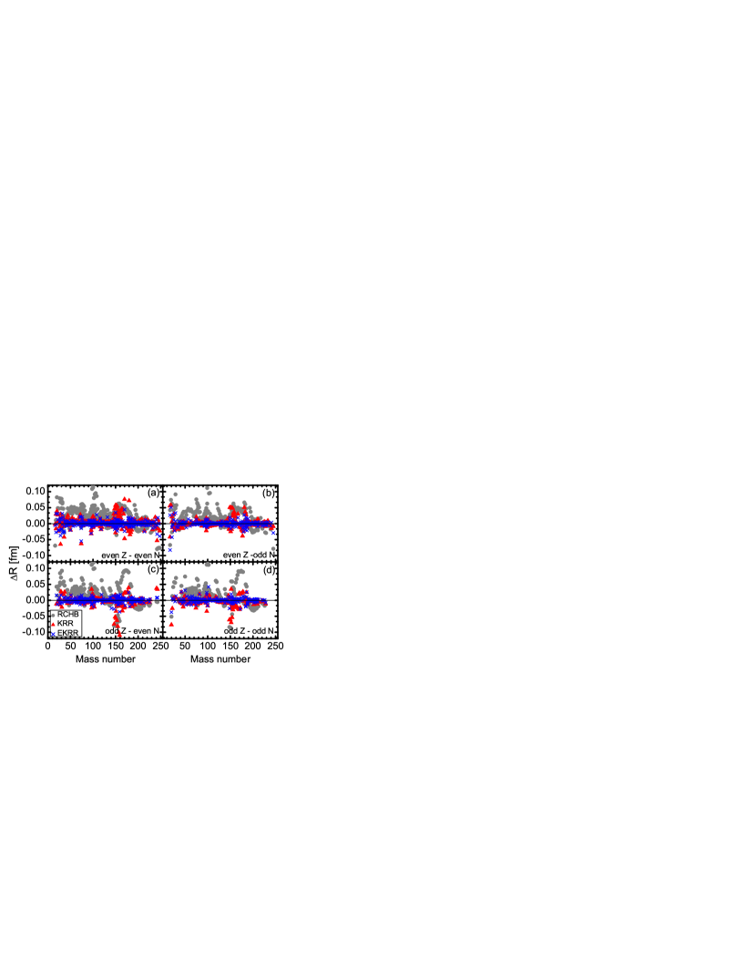
Figure 2: (Color online) Radius differences $\Delta R$ between the experimental data and the calculations of the RCHB model (grey solid circles), the KRR method (red triangles), and the EKRR method (blue crosses) for (a) even-even, (b) even-odd, (c) odd-even, and (d) odd-odd nuclei.

Figure 2 shows the differences in the radii between the experimental data and the calculations of the RCHB model (grey solid circles), KRR method (red triangles) and the EKRR methods (blue crosses). Because the improvements achieved by the KRR and EKRR methods for the five models mentioned above were similar, we consider only the RCHB model as an example. In order to study the odd-even effects included in the EKRR method, the data were divided into four groups characterized by even or odd proton numbers $Z$ and neutron numbers $N$, that is, even-even, even-odd, odd-even, and odd-odd. Clearly, the predictive power of the RCHB model could be further improved by using the EKRR method compared with the original KRR method. The significant improvement of the EKRR method is mainly due to the consideration of the odd-even effects, which eliminates the staggering behavior of radius deviations owing to the odd and even numbers of nucleons using the KRR method. It can be seen that when the mass number is $A\sim 150$, the predictions of the KRR method exhibit significant deviations from the data, which can be significantly improved using the EKRR method. This is clear evidence of the importance of considering the odd-even effects in predictions of the nuclear charge radius.

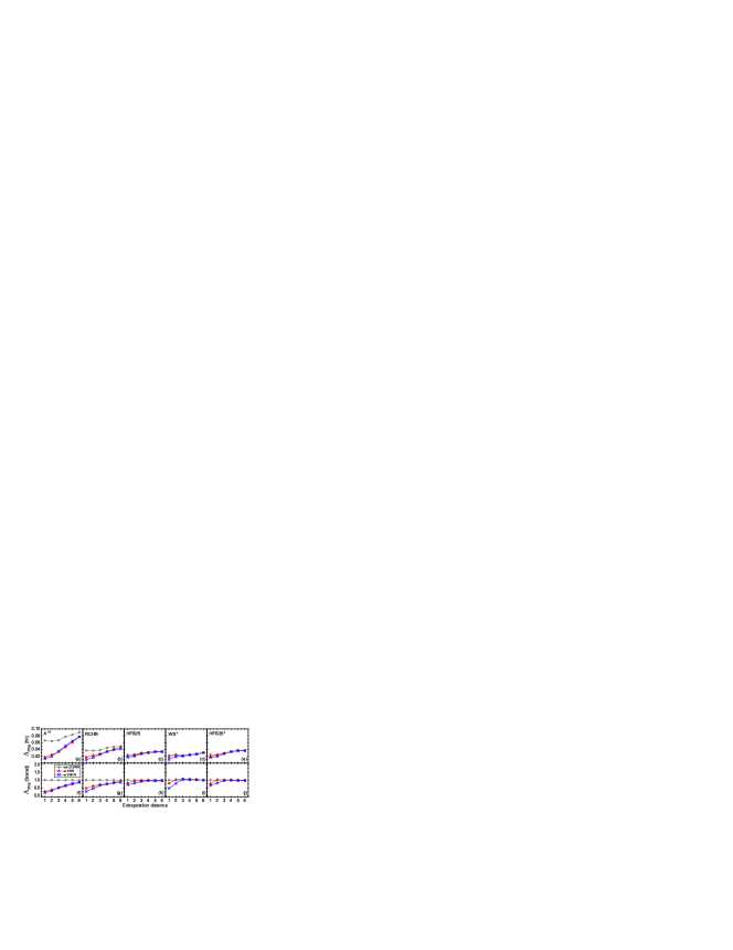
Figure 3: (Color online) Comparison of the extrapolation ability of the KRR and EKRR methods for the neutron-rich region by considering six test sets with different extrapolation distances. The upper panels (a)-(e) show the RMS deviations of the KRR and EKRR methods. The lower panels (f)-(j) show the RMS deviations scaled to the corresponding RMS deviations for these five models without KRR/EKRR corrections.

To investigate the extrapolation abilities of the KRR and EKRR methods for neutron-rich regions, the 1014 nuclei with known charge radii were redivided into one training set and six test sets as follows: For each isotopic chain with more than nine nuclei, the six most neutron-rich nuclei were selected and classified into six test sets based on the distance from the previous nucleus. Test set 1 (6) had the shortest (longest) extrapolation distance. This type of classification is the same as that used in our previous study Ma and Zhang (2022). The hyperparameters obtained by leave-one-out cross-validation in the KRR/RKRR method remained the same in the following calculations:

RMS deviations of the KRR and EKRR methods for different extrapolation steps for the five models are shown in Figs. 3(a)-(e). A clearer comparison of the RMS deviations scaled to the corresponding RMS deviations of the five models without KRR/EKRR corrections are shown in Figs. 3(f) and (j). Regardless of whether the KRR or EKRR method is considered, the RMS deviation increased with the extrapolation distance. For the $A^{1/3}$ formula and the RCHB model, the KRR/EKRR method could improve the radius description for all extrapolation distances. For the other three models, the KRR method only improved the radius description for an extrapolation distance of one or two, which could be further improved after considering the odd-even effects with the EKRR method. This indicates that the KRR/EKRR method loses its extrapolation power at extrapolation distances larger than 3 for these three models. This is due to the charge radii calculated using these three models, which were quite good, and their RMS deviations, which were already sufficiently small. The KRR/EKRR method automatically identifies the extrapolation distance limit owing to the hyperparameters $\sigma$ and $\sigma_{\rm oe}$ being optimized using the training data. Refs. Wu and Zhao (2020); Wu et al. (2021) demonstrated that the KRR and EKRR methods lose their predictive power at larger extrapolation distances (approximately six), when predicting the nuclear mass using the mass model WS4 Wang et al. (2014). This may be due to much more mass data existed than the charge radii, and the KRR/EKRR networks can be trained better with more data. In general, the EKRR method has a better predictive power than the KRR method for an extrapolation distance of less than 3. For an extrapolation distance greater than 3, the results of the KRR and EKRR methods were similar in most cases. Almost none of these extrapolations exhibited overfitting, except for WS^∗ at an extrapolation distance of 3, and this overfitting was quite small. This indicates that both the KRR and EKRR methods have good extrapolation powers and can avoid the risk of overfitting to a large extent.

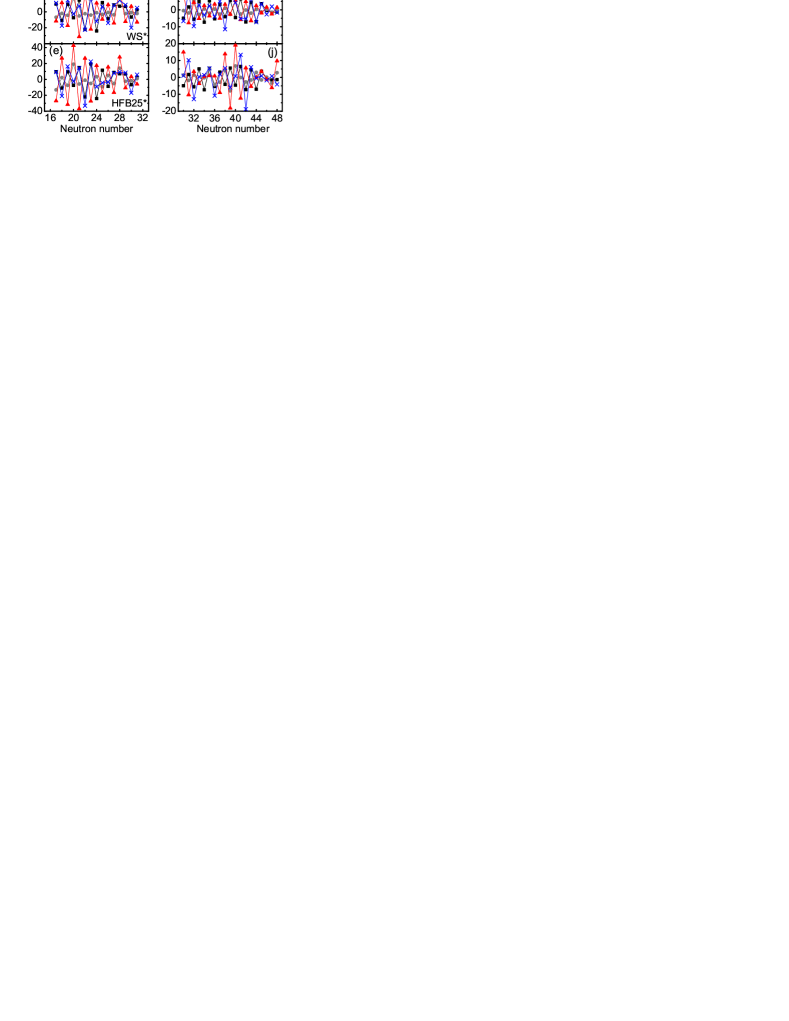
Figure 4: (Color online) Comparison of experimental and calculated OES of the charge radii ($\Delta^{(3)}_{r}$) of the calcium (left panels) and copper (right panels) isotopes. The experimental data are shown as black squares. The calculation results of these five models are shown as grey solid circles, and the calculation results of the KRR and EKRR models are shown as red triangles and blue crosses, respectively.

The observation of the strong OES of the charge radii throughout the nuclear landscape provides a particularly stringent test for nuclear theory. To examine the predictive power of the EKRR method, which is improved by considering the odd-even effects compared with the original KRR method, in the following we will investigate the recently observed OES of the radii in calcium and copper isotopes Ruiz et al. (2016); Miller et al. (2019); de Groote et al. (2020). Similar to the gap parameter, the OES parameter for the charge radii is defined as:

$$\Delta_{r}^{(3)}(Z,N)=\frac{1}{2}[r(Z,N-1)-2r(Z,N)+r(Z,N+1)]\ ,$$ (9)

where $r(Z,N)$ is the RMS charge radius of a nucleus with proton number $Z$ and neutron number $N$.

Figure 4 compares the experimental and calculated OES results for radii ($\Delta^{(3)}_{r}$) of the calcium (left panels) and copper (right panels) isotopes. The experimental data show that for the calcium isotopes [Figs. 4(a)-(e)] strong OES exists between $N=20$ and $28$ and that a reduction in the OES appears for $N\geq 28$. Only RCHB theory could reproduce the trend of the experimental OES without KRR/EKRR corrections. However, the amplitude of the calculated OES was significantly less pronounced than that of the experimental data. Interestingly, after considering the KRR corrections, the calculated OES worsened for $N<28$, particularly when the phase of the OES was opposite to that of the data. The $A^{1/3}$-formula had no OES over the entire isotopic chain and the WS^∗ model has a weak OES except at the $N=20$ and 28 shell closures. The OES in the HFB25 and HFB25^∗ models were slightly higher. However, they were still weak compared with the data. Note that although OES can be obtained in the WS^∗, HFB25 and HFB25^∗ models, the phases of the calculated OES are opposite to those of the experimental data. Considering the KRR method, the OES in these four models increased, particularly for the WS^∗ and HFB25^∗ models for which the calculated OES were stronger than those of the data. However, the OES in these models were still opposite to those in the data. Therefore, although the KRR method improves the description of the charge radius to a large extent, it was difficult to reproduce the observed OES. After considering the EKRR method, the experimental OES values could be reproduced quite well, especially for the $A^{1/3}$ formula and RCHB theory for copper isotopes [Figs. 4(f)-(j)]. This situation is similar to that of the calcium isotopes. However, the description of Cu isotopes is not as accurate as that of Ca isotopes when considering the EKRR corrections. The OES is overestimated in all these calculations for $N<33$ and $N>46$. In addition, the phases of the OES between $N=38$-40 were not well reproduced. However, the EKRR approach can improve the description of OES to a large extent compared with the original theory. This indicates that after considering the odd-even effects, shell structures and many-body correlations, which are important for OES, can be learned well using an EKRR network.

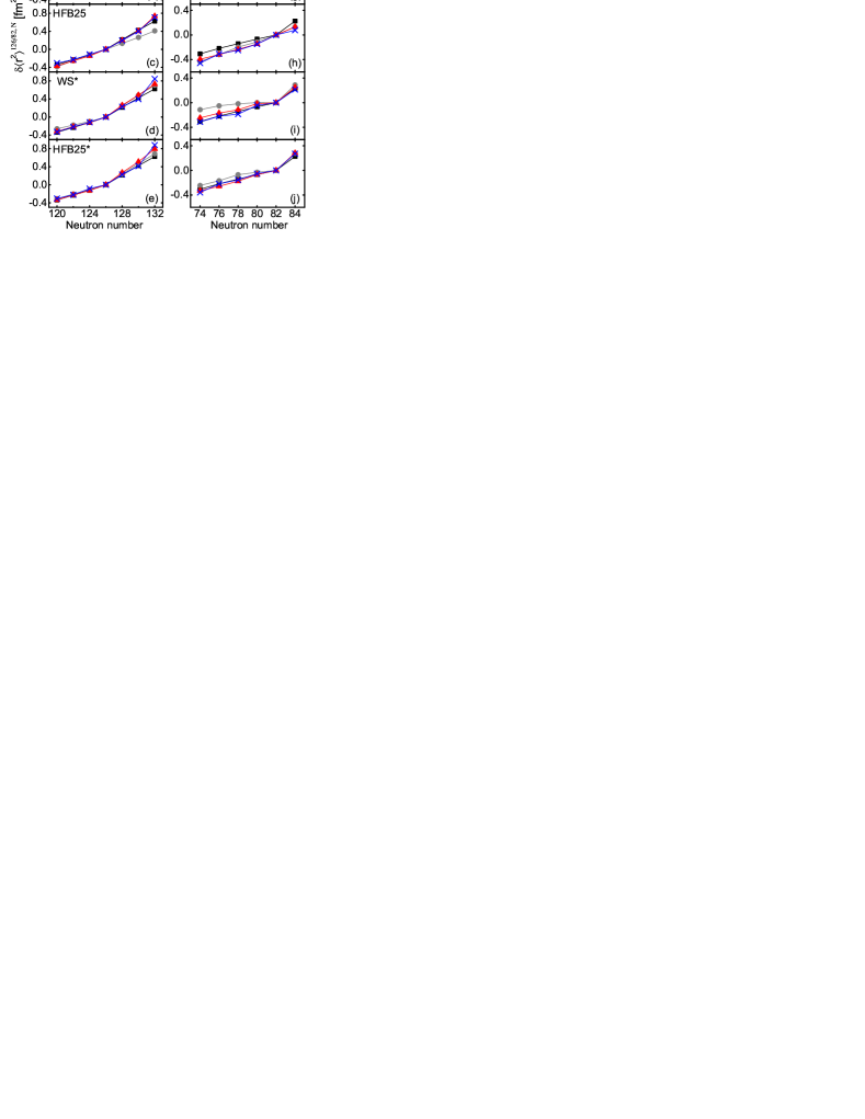
Figure 5: (Color online) Comparison of experimental and calculated differential mean-square charge radius $\delta\langle r^{2}\rangle^{N^{\prime},N}=\langle r^{2}\rangle^{N}-\langle r^{2}\rangle^{N^{\prime}}$ for some even-even (a)-(e) Pb (relative to ²⁰⁸Pb, $N^{\prime}=126$) and (f)-(j) Sn (relative to ¹³²Sn, $N^{\prime}=82$) isotopes. The experimental data are shown as black squares. The results of these five models are shown as grey solid circles, and the calculation results of the KRR and EKRR models are shown as red triangles and blue crosses, respectively.

Similar to OES, abrupt kinks across the neutron shell closures provide a particularly stringent test for nuclear theory. In the present study, Pb and Sn isotopes were considered as examples for investigating the kinks across neutrons with $N=126$ and 82 shell closures. Figure 5 compares the experimental and calculated differential mean-square charge radii. $\delta\langle r^{2}\rangle^{N^{\prime},N}=\langle r^{2}\rangle^{N}-\langle r^{2}\rangle^{N^{\prime}}$ for some, and even for Pb [Figs. 5(a)-(e)] (relative to ²⁰⁸Pb, $N^{\prime}=126$) and Sn [Figs. 5(f)-(j)] (relative to ¹³²Sn, $N^{\prime}=82$). It can be observed that for Pb isotopes the RCHB theory can reproduce the kink at $N=126$ perfectly [Fig. 5(b)]. In the $A^{1/3}$ formula and HFB25 model, there is no kink [Figs. 5(a) and (c)]. The kink could be reproduced using the WS^∗ and HFB25^∗ models, but with a slight overestimation [Figs. 5(d) and (e)]. The results obtained by considering the KRR and EKRR methods were similar. There are several interpretations of kinks Sharma et al. (1995); Perera et al. (2021); Nakada and Inakura (2015); Nakada (2015); Fayans et al. (2000). Our results indicate that kinks may not be connected to odd-even effects, such as pairing correlations. The well-reproduced kinks also provide a test of the proposed KRR/EKRR method. The kinks at $N=126$ in all five models could be reproduced quite well, but the calculated differential mean-square charge radius at $N=132$ was too large compared with the data. For the Sn isotopes, only the WS^∗ and HFB25^∗ models reproduced the kink at $N=82$. However, the absolute values of the calculated $\delta\langle r^{2}\rangle$ from $N=74$-78 are small compared with the data, especially for the WS^∗ model. After applying the KRR/EKRR method, the results reproduced the data quite well. It also can be seen that the KRR/EKRR corrections to the $A^{1/3}$ formula and HFB25 model are inconspicuous. Therefore, the kink at $N=82$ cannot be reproduced using the KRR/EKRR method. For the RCHB model, the differential mean-square charge radii calculated from $N=74$ to-80 were improved, and a kink appeared, but was still slightly weaker compared with the data.

V Summary

In summary, the extended kernel ridge regression method with odd-even effects was adopted to improve the description of the nuclear charge radius by using five commonly used nuclear models. The hyperparameters of the KRR and EKRR methods for each model were determined using leave-one-out cross-validation. For each model, the resultant root-mean-square deviations of the 1014 nuclei with proton number $Z\geq 8$ could be significantly reduced to 0.009-0.013 fm after considering a modification with the EKRR method. The best among them was the RCHB model, with a root-mean-square deviation of 0.0092 fm, which is the best result for nuclear charge radii predictions using the machine learning approach as far as we know. The extrapolation abilities of the KRR and EKRR methods for the neutron-rich region were examined and it was found that after considering odd-even effects, the extrapolation power could be improved compared with that of the original KRR method. Strong odd-even staggering of nuclear charge radii in Ca and Cu isotopes was investigated and reproduced quite well using the EKRR method. This indicates that after considering the odd-even effects, shell structures and many-body correlations can be learned quite well using the EKRR network. Abrupt kinks across the neutron $N=126$ and 82 shell closures were also investigated.

References

- Angeli and Marinova (2015) I. Angeli and K. P. Marinova, J. Phys. G: Nucl. Part. Phys. 42, 055108 (2015).
- Gorges et al. (2019) C. Gorges, L. V. Rodríguez, D. L. Balabanski, M. L. Bissell, K. Blaum, B. Cheal, R. F. Garcia Ruiz, G. Georgiev, W. Gins, H. Heylen, A. Kanellakopoulos, S. Kaufmann, M. Kowalska, V. Lagaki, S. Lechner, B. Maaß, S. Malbrunot-Ettenauer, W. Nazarewicz, R. Neugart, G. Neyens, W. Nörtershäuser, P.-G. Reinhard, S. Sailer, R. Sánchez, S. Schmidt, L. Wehner, C. Wraith, L. Xie, Z. Y. Xu, X. F. Yang, and D. T. Yordanov, Phys. Rev. Lett. 122, 192502 (2019).
- Wood et al. (1992) J. L. Wood, K. Heyde, W. Nazarewicz, M. Huyse, and P. van Duppen, Phys. Rep. 215, 101 (1992).
- Cejnar et al. (2010) P. Cejnar, J. Jolie, and R. F. Casten, Rev. Mod. Phys. 82, 2155 (2010).
- Tanihata et al. (1985) I. Tanihata, H. Hamagaki, O. Hashimoto, Y. Shida, N. Yoshikawa, K. Sugimoto, O. Yamakawa, T. Kobayashi, and N. Takahashi, Phys. Rev. Lett. 55, 2676 (1985).
- Tanihata et al. (2013) I. Tanihata, H. Savajols, and R. Kanungo, Prog. Part. Nucl. Phys. 68, 215 (2013).
- Meng and Zhou (2015) J. Meng and S. G. Zhou, J. Phys. G: Nucl. Part. Phys. 42, 093101 (2015).
- Cheal and Flanagan (2010) B. Cheal and K. T. Flanagan, J. Phys. G: Nucl. Part. Phys. 37, 113101 (2010).
- Campbell et al. (2016) P. Campbell, I. D. Moore, and M. R. Pearson, Prog. Part. Nucl. Phys. 86, 127 (2016).
- Angeli and Marinova (2013) I. Angeli and K. Marinova, At. Data Nucl. Data Tables 99, 69 (2013).
- Li et al. (2021) T. Li, Y. Luo, and N. Wang, At. Data Nucl. Data Tables 140, 101440 (2021).
- Goddard et al. (2013) P. M. Goddard, P. D. Stevenson, and A. Rios, Phys. Rev. Lett. 110, 032503 (2013).
- Hammen et al. (2018) M. Hammen, W. Nörtershäuser, D. L. Balabanski, M. L. Bissell, K. Blaum, I. Budinčević, B. Cheal, K. T. Flanagan, N. Frömmgen, G. Georgiev, C. Geppert, M. Kowalska, K. Kreim, A. Krieger, W. Nazarewicz, R. Neugart, G. Neyens, J. Papuga, P.-G. Reinhard, M. M. Rajabali, S. Schmidt, and D. T. Yordanov, Phys. Rev. Lett. 121, 102501 (2018).
- Ruiz et al. (2016) G. Ruiz, R. F., M. L. Bissell, K. Blaum, A. Ekström, N. Frömmgen, G. Hagen, M. Hammen, K. Hebeler, J. D. Holt, G. R. Jansen, M. Kowalska, K. Kreim, W. Nazarewicz, R. Neugart, G. Neyens, W. Nörtershäuser, T. Papenbrock, J. Papuga, A. Schwenk, J. Simonis, K. A. Wendt, and D. T. Yordanov, Nat. Phys. 12, 594 (2016).
- Miller et al. (2019) A. J. Miller, K. Minamisono, A. Klose, D. Garand, C. Kujawa, J. D. Lantis, Y. Liu, B. Maaß, P. F. Mantica, W. Nazarewicz, W. Nörtershäuser, S. V. Pineda, P.-G. Reinhard, D. M. Rossi, F. Sommer, C. Sumithrarachchi, A. Teigelhöfer, and J. Watkins, Nat. Phys. 15, 432 (2019).
- de Groote et al. (2020) P. R. de Groote, J. Billowes, C. L. Binnersley, M. L. Bissell, T. E. Cocolios, T. Day Goodacre, G. J. Farooq-Smith, D. V. Fedorov, K. T. Flanagan, S. Franchoo, R. F. Garcia Ruiz, W. Gins, J. D. Holt, A. Koszorús, K. M. Lynch, T. Miyagi, W. Nazarewicz, G. Neyens, P.-G. Reinhard, S. Rothe, H. H. Stroke, A. R. Vernon, K. D. A. Wendt, S. G. Wilkins, Z. Y. Xu, and X. F. Yang, Nat. Phys. 16, 620 (2020).
- Day Goodacre et al. (2021) T. Day Goodacre, A. V. Afanasjev, A. E. Barzakh, B. A. Marsh, S. Sels, P. Ring, H. Nakada, A. N. Andreyev, P. Van Duppen, N. A. Althubiti, B. Andel, D. Atanasov, J. Billowes, K. Blaum, T. E. Cocolios, J. G. Cubiss, G. J. Farooq-Smith, D. V. Fedorov, V. N. Fedosseev, K. T. Flanagan, L. P. Gaffney, L. Ghys, M. Huyse, S. Kreim, D. Lunney, K. M. Lynch, V. Manea, Y. Martinez Palenzuela, P. L. Molkanov, M. Rosenbusch, R. E. Rossel, S. Rothe, L. Schweikhard, M. D. Seliverstov, P. Spagnoletti, C. Van Beveren, M. Veinhard, E. Verstraelen, A. Welker, K. Wendt, F. Wienholtz, R. N. Wolf, A. Zadvornaya, and K. Zuber, Phys. Rev. Lett. 126, 032502 (2021).
- Reponen et al. (2021) M. Reponen, R. P. de Groote, L. Al Ayoubi, O. Beliuskina, M. L. Bissell, P. Campbell, L. Cañete, B. Cheal, K. Chrysalidis, C. Delafosse, A. de Roubin, C. S. Devlin, T. Eronen, R. F. Garcia Ruiz, S. Geldhof, W. Gins, M. Hukkanen, P. Imgram, A. Kankainen, M. Kortelainen, A. Koszorús, S. Kujanpää, R. Mathieson, D. A. Nesterenko, I. Pohjalainen, M. Vilén, A. Zadvornaya, and I. D. Moore, Nat. Commun. 12, 4596 (2021).
- Koszorús et al. (2021) A. Koszorús, X. F. Yang, W. G. Jiang, S. J. Novario, S. W. Bai, J. Billowes, C. L. Binnersley, M. L. Bissell, T. E. Cocolios, B. S. Cooper, R. P. de Groote, A. Ekström, K. T. Flanagan, C. Forssén, S. Franchoo, R. F. G. Ruiz, F. P. Gustafsson, G. Hagen, G. R. Jansen, A. Kanellakopoulos, M. Kortelainen, W. Nazarewicz, G. Neyens, T. Papenbrock, P.-G. Reinhard, C. M. Ricketts, B. K. Sahoo, A. R. Vernon, and S. G. Wilkins, Nat. Phys. 17, 439 (2021).
- Malbrunot-Ettenauer et al. (2022) S. Malbrunot-Ettenauer, S. Kaufmann, S. Bacca, C. Barbieri, J. Billowes, M. L. Bissell, K. Blaum, B. Cheal, T. Duguet, R. F. G. Ruiz, W. Gins, C. Gorges, G. Hagen, H. Heylen, J. D. Holt, G. R. Jansen, A. Kanellakopoulos, M. Kortelainen, T. Miyagi, P. Navrátil, W. Nazarewicz, R. Neugart, G. Neyens, W. Nörtershäuser, S. J. Novario, T. Papenbrock, T. Ratajczyk, P.-G. Reinhard, L. V. Rodríguez, R. Sánchez, S. Sailer, A. Schwenk, J. Simonis, V. Somà, S. R. Stroberg, L. Wehner, C. Wraith, L. Xie, Z. Y. Xu, X. F. Yang, and D. T. Yordanov, Phys. Rev. Lett. 128, 022502 (2022).
- Geldhof et al. (2022) S. Geldhof, M. Kortelainen, O. Beliuskina, P. Campbell, L. Caceres, L. Cañete, B. Cheal, K. Chrysalidis, C. S. Devlin, R. P. de Groote, A. de Roubin, T. Eronen, Z. Ge, W. Gins, A. Koszorus, S. Kujanpää, D. Nesterenko, A. Ortiz-Cortes, I. Pohjalainen, I. D. Moore, A. Raggio, M. Reponen, J. Romero, and F. Sommer, Phys. Rev. Lett. 128, 152501 (2022).
- Bohr and Mottelson (1969) A. Bohr and B. R. Mottelson, Nuclear Structure, Vol. I Single-particle Motion (Benjamin, 1969).
- Zeng (1957) J. Y. Zeng, Acta Phys. Sin. 13, 357 (1957).
- Nerlo-Pomorska and Pomorski (1993) B. Nerlo-Pomorska and K. Pomorski, Z. Phys. A 344, 359 (1993).
- Duflo (1994) J. Duflo, Nucl. Phys. A 576, 29 (1994).
- Zhang et al. (2002) S. Zhang, J. Meng, S.-G. Zhou, and J. Zeng, Eur. Phys. J. A 13, 285 (2002).
- Lei et al. (2009) Y.-A. Lei, Z.-H. Zhang, and J.-Y. Zeng, Commun. Theor. Phys. 51, 123 (2009).
- Wang and Li (2013) N. Wang and T. Li, Phys. Rev. C 88, 011301(R) (2013).
- Bayram et al. (2013) T. Bayram, S. Akkoyun, S. Kara, and A. Sinan, Acta Phys. Pol. B 44, 1791 (2013).
- Piekarewicz et al. (2010) J. Piekarewicz, M. Centelles, X. Roca-Maza, and X. Viñas, Eur. Phys. J. A 46, 379 (2010).
- Sun et al. (2014) B. H. Sun, Y. Lu, J. P. Peng, C. Y. Liu, and Y. M. Zhao, Phys. Rev. C 90, 054318 (2014).
- Bao et al. (2016) M. Bao, Y. Lu, Y. M. Zhao, and A. Arima, Phys. Rev. C 94, 064315 (2016).
- Sun et al. (2017) B. H. Sun, C. Y. Liu, and H. X. Wang, Phys. Rev. C 95, 014307 (2017).
- Bao et al. (2020) M. Bao, Y. Y. Zong, Y. M. Zhao, and A. Arima, Phys. Rev. C 102, 014306 (2020).
- Ma et al. (2021) C. Ma, Y. Y. Zong, Y. M. Zhao, and A. Arima, Phys. Rev. C 104, 014303 (2021).
- Buchinger et al. (1994) F. Buchinger, J. E. Crawford, A. K. Dutta, J. M. Pearson, and F. Tondeur, Phys. Rev. C 49, 1402 (1994).
- Buchinger et al. (2001) F. Buchinger, J. M. Pearson, and S. Goriely, Phys. Rev. C 64, 067303 (2001).
- Buchinger and Pearson (2005) F. Buchinger and J. M. Pearson, Phys. Rev. C 72, 057305 (2005).
- Iimura and Buchinger (2008) H. Iimura and F. Buchinger, Phys. Rev. C 78, 067301 (2008).
- Stoitsov et al. (2003) M. V. Stoitsov, J. Dobaczewski, W. Nazarewicz, S. Pittel, and D. J. Dean, Phys. Rev. C 68, 054312 (2003).
- Goriely et al. (2009) S. Goriely, S. Hilaire, M. Girod, and S. Péru, Phys. Rev. Lett. 102, 242501 (2009).
- Goriely et al. (2010) S. Goriely, N. Chamel, and J. M. Pearson, Phys. Rev. C 82, 035804 (2010).
- Reinhard and Nazarewicz (2017) P.-G. Reinhard and W. Nazarewicz, Phys. Rev. C 95, 064328 (2017).
- Lalazissis et al. (1999) G. A. Lalazissis, S. Raman, and P. Ring, At. Data Nucl. Data Tables 71, 1 (1999).
- Geng et al. (2005) L. S. Geng, H. Toki, and J. Meng, Prog. Theo. Phys. 113, 785 (2005).
- Zhao et al. (2010) P. W. Zhao, Z. P. Li, J. M. Yao, and J. Meng, Phys. Rev. C 82, 054319 (2010).
- Xia et al. (2018) X. W. Xia, Y. Lim, P. W. Zhao, H. Z. Liang, X. Y. Qu, Y. Chen, H. Liu, L. F. Zhang, S. Q. Zhang, Y. Kim, and J. Meng, At. Data Nucl. Data Tables 121-122, 1 (2018).
- Zhang et al. (2020) K. Zhang, M.-K. Cheoun, Y.-B. Choi, P. S. Chong, J. Dong, L. Geng, E. Ha, X. He, C. Heo, M. C. Ho, E. J. In, S. Kim, Y. Kim, C.-H. Lee, J. Lee, Z. Li, T. Luo, J. Meng, M.-H. Mun, Z. Niu, C. Pan, P. Papakonstantinou, X. Shang, C. Shen, G. Shen, W. Sun, X.-X. Sun, C. K. Tam, Thaivayongnou, C. Wang, S. H. Wong, X. Xia, Y. Yan, R. W.-Y. Yeung, T. C. Yiu, S. Zhang, W. Zhang, and S.-G. Zhou (DRHBc Mass Table Collaboration), Phys. Rev. C 102, 024314 (2020).
- An et al. (2020) R. An, L.-S. Geng, and S.-S. Zhang, Phys. Rev. C 102, 024307 (2020).
- Perera et al. (2021) U. C. Perera, A. V. Afanasjev, and P. Ring, Phys. Rev. C 104, 064313 (2021).
- Zhang et al. (2022) K. Zhang, M.-K. Cheoun, Y.-B. Choi, P. S. Chong, J. Dong, Z. Dong, X. Du, L. Geng, E. Ha, X.-T. He, C. Heo, M. C. Ho, E. J. In, S. Kim, Y. Kim, C.-H. Lee, J. Lee, H. Li, Z. Li, T. Luo, J. Meng, M.-H. Mun, Z. Niu, C. Pan, P. Papakonstantinou, X. Shang, C. Shen, G. Shen, W. Sun, X.-X. Sun, C. K. Tam, Thaivayongnou, C. Wang, X. Wang, S. H. Wong, J. Wu, X. Wu, X. Xia, Y. Yan, R. W.-Y. Yeung, T. C. Yiu, S. Zhang, W. Zhang, X. Zhang, Q. Zhao, and S.-G. Zhou, At. Data Nucl. Data Tables 144, 101488 (2022).
- An et al. (2023) R. An, S. Sun, L.-G. Cao, and F.-S. Zhang, Nucl. Sci. Tech. 34, 119 (2023).
- Forssén et al. (2009) C. Forssén, E. Caurier, and P. Navrátil, Phys. Rev. C 79, 021303(R) (2009).
- Choudhary et al. (2020) P. Choudhary, P. C. Srivastava, and P. Navrátil, Phys. Rev. C 102, 044309 (2020).
- Bedaque et al. (2021) P. Bedaque, A. Boehnlein, M. Cromaz, M. Diefenthaler, L. Elouadrhiri, T. Horn, M. Kuchera, D. Lawrence, D. Lee, S. Lidia, R. McKeown, W. Melnitchouk, W. Nazarewicz, K. Orginos, Y. Roblin, M. Scott Smith, M. Schram, and X.-N. Wang, Eur. Phys. J. A 57, 100 (2021).
- Boehnlein et al. (2022) A. Boehnlein, M. Diefenthaler, N. Sato, M. Schram, V. Ziegler, C. Fanelli, M. Hjorth-Jensen, T. Horn, M. P. Kuchera, D. Lee, W. Nazarewicz, P. Ostroumov, K. Orginos, A. Poon, X.-N. Wang, A. Scheinker, M. S. Smith, and L.-G. Pang, Rev. Mod. Phys. 94, 031003 (2022).
- He et al. (2023a) W.-B. He, Y.-G. Ma, L.-G. Pang, H.-C. Song, and K. Zhou, Nucl. Sci. Tech. 34, 88 (2023a).
- He et al. (2023b) W. He, Q. Li, Y. Ma, Z. Niu, J. Pei, and Y. Zhang, Sci. China-Phys. Mech. Astron. 66, 282001 (2023b).
- Gao et al. (2021) Z.-P. Gao, Y.-J. Wang, H.-L. Lü, Q.-F. Li, C.-W. Shen, and L. Liu, Nucl. Sci. Tech. 32, 109 (2021).
- Akkoyun et al. (2013) S. Akkoyun, T. Bayram, S. O. Kara, and A. Sinan, J. Phys. G: Nucl. Part. Phys. 40, 055106 (2013).
- Wu et al. (2020) D. Wu, C. L. Bai, H. Sagawa, and H. Q. Zhang, Phys. Rev. C 102, 054323 (2020).
- Shang et al. (2022) T.-S. Shang, J. Li, and Z.-M. Niu, Nucl. Sci. Tech. 33, 153 (2022).
- Yang et al. (2023) Z.-X. Yang, X.-H. Fan, T. Naito, Z.-M. Niu, Z.-P. Li, and H. Liang, Phys. Rev. C 108, 034315 (2023).
- Utama et al. (2016) R. Utama, W.-C. Chen, and J. Piekarewicz, J. Phys. G: Nucl. Part. Phys. 43, 114002 (2016).
- Neufcourt et al. (2018) L. Neufcourt, Y. Cao, W. Nazarewicz, and F. Viens, Phys. Rev. C 98, 034318 (2018).
- Ma et al. (2020) Y. Ma, C. Su, J. Liu, Z. Ren, C. Xu, and Y. Gao, Phys. Rev. C 101, 014304 (2020).
- Dong et al. (2022) X.-X. Dong, R. An, J.-X. Lu, and L.-S. Geng, Phys. Rev. C 105, 014308 (2022).
- Dong et al. (2023) X.-X. Dong, R. An, J.-X. Lu, and L.-S. Geng, Phys. Lett. B 838, 137726 (2023).
- Li et al. (2023) T. Li, H. Yao, M. Liu, and N. Wang, Nucl. Phys. Rev. 40, 31 (2023), (in Chinese).
- Ma and Zhang (2022) J.-Q. Ma and Z.-H. Zhang, Chin. Phys. C 46, 074105 (2022).
- Kim et al. (2012) N. Kim, Y.-S. Jeong, M.-K. Jeong, and T. M. Young, IEEE Trans. Syst. Man Cybern. 42, 1011 (2012).
- Wu et al. (2017) P.-Y. Wu, C.-C. Fang, J. M. Chang, and S.-Y. Kung, IEEE Trans. Cybern 47, 3916 (2017).
- Wu and Zhao (2020) X. H. Wu and P. W. Zhao, Phys. Rev. C 101, 051301(R) (2020).
- Wu et al. (2021) X. H. Wu, L. H. Guo, and P. W. Zhao, Phys. Lett. B 819, 136387 (2021).
- Guo et al. (2022) L. Guo, X. Wu, and P. Zhao, Symmetry 14, 1078 (2022).
- Wu et al. (2022a) X. H. Wu, Y. Y. Lu, and P. W. Zhao, Phys. Lett. B 834, 137394 (2022a).
- Du et al. (2023) X. Du, P. Guo, X. Wu, and S. Zhang, Chin. Phys. C 47, 074108 (2023).
- Wu et al. (2022b) X. H. Wu, Z. X. Ren, and P. W. Zhao, Phys. Rev. C 105, L031303 (2022b).
- Huang et al. (2022) T. X. Huang, X. H. Wu, and P. W. Zhao, Commun. Theor. Phys. 74, 095302 (2022).
- Goriely et al. (2013) S. Goriely, N. Chamel, and J. M. Pearson, Phys. Rev. C 88, 024308 (2013).
- Wang et al. (2014) N. Wang, M. Liu, X. Wu, and J. Meng, Phys. Lett. B 734, 215 (2014).
- Sharma et al. (1995) M. M. Sharma, G. Lalazissis, J. König, and P. Ring, Phys. Rev. Lett. 74, 3744 (1995).
- Nakada and Inakura (2015) H. Nakada and T. Inakura, Phys. Rev. C 91, 021302(R) (2015).
- Nakada (2015) H. Nakada, Phys. Rev. C 92, 044307 (2015).
- Fayans et al. (2000) S. A. Fayans, S. V. Tolokonnikov, E. L. Trykov, and D. Zawischa, Nucl. Phys. A 676, 49 (2000).