Latent Concept-based Explanation of NLP Models

Abstract

Interpreting and understanding the predictions made by deep learning models poses a formidable challenge due to their inherently opaque nature. Many previous efforts aimed at explaining these predictions rely on input features, specifically, the words within NLP models. However, such explanations are often less informative due to the discrete nature of these words and their lack of contextual verbosity. To address this limitation, we introduce the Latent Concept Attribution method (LACOAT), which generates explanations for predictions based on latent concepts. Our foundational intuition is that a word can exhibit multiple facets, contingent upon the context in which it is used. Therefore, given a word in context, the latent space derived from our training process reflects a specific facet of that word. LACOAT functions by mapping the representations of salient input words into the training latent space, allowing it to provide predictions with context-based explanations within this latent space.

Latent Concept-based Explanation of NLP Models

Xuemin Yu Faculty of Computer Science, Dalhousie University, Canada xuemin.yu@dal.ca                        Fahim Dalvi Qatar Computing Research Institute, HBKU, Qatar faimaduddin@hbku.edu.qa

Nadir Durrani Qatar Computing Research Institute, HBKU, Qatar ndurrani@hbku.edu.qa                        Hassan Sajjad Faculty of Computer Science, Dalhousie University, Canada hsajjad@dal.ca

1 Introduction

The opaqueness of deep neural network (DNN) models is a major challenge to ensuring a safe and trustworthy AI system. Extensive and diverse research works have attempted to interpret and explain these models. One major line of work strives to understand and explain the prediction of a neural network model using the attribution of input words to prediction Sundararajan et al. (2017a); Denil et al. (2014).

However, the explanation based solely on input words is less informative due to the discrete nature of words and the lack of contextual verbosity. A word consists of multifaceted aspects such as semantic, morphological, and syntactic roles in a sentence. Consider the word “trump” in Figure 1. It has several facets such as a verb, a verb with specific semantics, a named entity and a named entity representing a certain aspect such as tower names, family names, etc. We argue that given various contexts of a word in the training data, the model learns these diverse facets during training. Given a test instance, depending on the context a word appears, the model uses a particular facet of the input words in making the prediction. The explanation based on salient words alone does not reflect the facets of the word the model has used in the prediction and results in a less informed explanation.

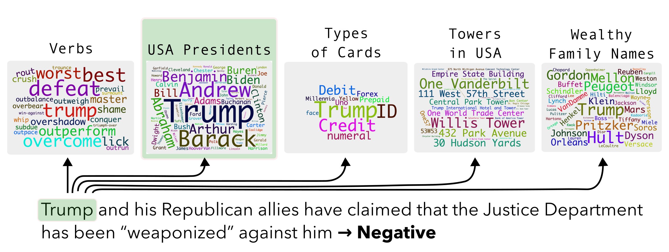
Figure 1: An example of various facets of word “trump”

Dalvi et al. (2022) showed that the latent space of DNNs represents the multifaceted aspects of words learned during training. The clustering of training data contextualized representations provides access to these multifaceted concepts, hereafter referred to as latent concepts. Given an input word in context at test time, we hypothesize that the alignment of its contextualized representation to a latent concept represents the facet of the word being used by the model for that particular input. We further hypothesize that this latent concept serves as a correct and enriched explanation of the input word. To this end, we propose the LAtent COncept ATtribution (LACOAT) method that generates an explanation of a model’s prediction using the latent concepts. LACOAT discovers latent concepts of every layer of the model by clustering contextualized representations of words in the training corpus. Given a test instance, it identifies the most salient input representations of every layer with respect to the prediction and dynamically maps them to the latent concepts of the training data. The shortlisted latent concepts serve as an explanation of the prediction. Lastly, LACOAT integrates a plausibility module that generates a human-friendly explanation of the latent concept-based explanation.

LACOAT is a local explanation method that provides an explanation of a single test instance. The reliance on the training data latent space makes the explanation reliable and further reflects on the quality of learning of the model and the training data. We perform qualitative and quantitative evaluation of LACOAT using the part-of-speech (POS) tagging and sentiment classification tasks across three pre-trained models. LACOAT generates an enriched explanation that is useful in understanding the model’s reasoning for a prediction. It also helps in understanding how the model has structured the knowledge of a task. We also conduct human evaluation to measure the utility of LACOAT with a human-in-the-loop.

2 Methodology

LACOAT consists of the following four modules:

• The first module, ConceptDiscoverer, discovers latent concepts of a model given a corpus.

• PredictionAttributor, the second module, selects the most salient words (along with their contextual representations) in a sentence with respect to the model’s prediction.

• Thirdly, ConceptMapper, maps the representations of the salient words to the latent concepts discovered by ConceptDiscoverer and provides a latent concept-based explanation.

• PlausiFyer takes a latent concept explanation as input and generates a plausible and human-understandable explanation of the prediction.

Consider a sentiment classification dataset and a sentiment classification model as an example. LACOAT works as follows: ConceptDiscoverer takes the training dataset and the model as input and outputs latent concepts of the model. At test time, given an input sentence, PredictionAttributor identifies the most salient input representations with respect to the prediction. ConceptMapper maps these salient input representations to the training data latent concepts and provides them as an explanation of the prediction. PlausiFyer takes the test sentence and its concept-based explanation and generates a human-friendly and insightful explanation of the prediction. In the following we describe these modules in detail.

Consider $\mathbb{M}$ represents the DNN model being interpreted, with $L$ layers, each of size $H$. Let $\overrightarrow{z}_{w_{i}}$ be the contextual representation of a word $w_{i}$ in an input sentence $\{w_{1},w_{2},...,w_{i},....\}$. The representation can belong to any particular layer in the model, and LACOAT will generate explanations with respect to that layer.

2.1 ConceptDiscoverer

The words are grouped in the high-dimensional space based on various latent relations such as semantic, morphology and syntax Mikolov et al. (2013); Reif et al. (2019). With the inclusion of context i.e. contextualized representations, these groupings evolve into dynamically formed clusters representing a unique facet of the words called latent concept Dalvi et al. (2022). Figure 1 shows a few examples of latent concepts that capture different facets of the word "trump".

The goal of ConceptDiscoverer is to discover latent concepts given a model $\mathbb{M}$ and a dataset $\mathbb{D}$. We follow an identical procedure to Dalvi et al. (2022) to discover latent concepts. Specifically, for every word $w_{i}$ in $\mathbb{D}$, we extract contextual representations $\overrightarrow{z}_{w_{i}}$. We then cluster these representations using agglomerative hierarchical clustering Gowda and Krishna (1978). Specifically, the distance between any two representations is computed using the squared Euclidean distance, and Ward’s minimum variance criterion is used to minimize total within-cluster variance.

Each cluster represents a latent concept. Let $\mathcal{C}={C_{1},C_{2},...,C_{K}}$ represents the set of latent concepts extracted by ConceptDiscoverer, where each $C_{i}={w_{1},w_{2},...}$ is a set of words in a particular context. For sequence classification tasks, we also consider the [CLS] token (or a representative classification token) from each sentence in the dataset as a “word” and discover the latent concepts. In this case, a latent concept may consist of words only, [CLS] tokens only, or a mix of both.

2.2 Salient Representations Extraction

Given an input instance $s$, the goal of PredictionAttributor is to extract salient input representations with respect to the prediction $p$ from model $\mathbb{M}$. Gradient-based methods have been effectively used to compute the saliency of the input features for the given prediction, such as pure Gradient Simonyan et al. (2014), Input x Gradient Shrikumar et al. (2017) and Integrated Gradients (IG) Sundararajan et al. (2017b). In this work, we use IG as our gradient-based method as it’s a well-established method from literature. However, LACOAT is agnostic to the choice of the attribution method, and any other method that identifies salient input representations can be used while keeping the rest of the pipeline unchanged.

Formally, we first use IG to get attribution scores for every token in the input $s$, and then select the top tokens that make up $50\%$ of the total attribution mass (similar to top-P sampling).

In addition to the saliency based attribution method, we also experimented with using the position of the output head as an indication of the most salient contextual representation. A detailed description and results are provided in Appendix A.

2.3 ConceptMapper

At test time, given an input sentence PredictionAttributor provides the salient input representations. ConceptMapper maps each salient representation to a latent concept $C_{i}$ of the training latent space. These latent concepts highlight a particular facet of the salient representations that is being used by the model and serve as an explanation of the prediction.

ConceptMapper uses a logistic regression classifier that maps a representation $\overrightarrow{z}_{w_{i}}$ to one of the $K$ latent concepts. The model is trained using the representations of words from $\mathbb{D}$ that are used by ConceptDiscoverer as input features and the concept index (cluster id) as their label. Hence, for a concept $C_{i}$ and a word $w_{j}\in C_{i}$, a training instance of the classifier is the input $x=\overrightarrow{z}_{w_{j}}$ and the output is $y=i$.

2.4 PlausiFyer

Interpreting latent concepts can be challenging due to the need for diverse knowledge, including linguistic, task-specific, worldly, and geographical expertise (as seen in Figure 1). PlausiFyer offers a user-friendly summary and explanation of the latent concept and its relationship to the input instance using a Large Language Model (LLM).

We use the following prompt for the sequence classification task:

Do you find any common semantic, structural, lexi-
cal and topical relation between these sentences
with the main sentence? Give a more specific and
concise summary about the most prominent relation
among these sentences.

main sentence: {sentence}
{sentences}
No talk, just go.

and the following prompt for the sequence labeling task:

Do you find any common semantic, structural, lexi-
cal and topical relation between the word highlig-
hted in the sentence (enclosed in [[ ]]) and the
following list of words? Give a more specific and
concise summary about the most prominent relation
among these words.

Sentence: {sentence}
List of words: {words}
Answer concisely and to the point.

We did not provide the prediction or the gold label to LLM to avoid biasing the explanation.

3 Experimental Setup

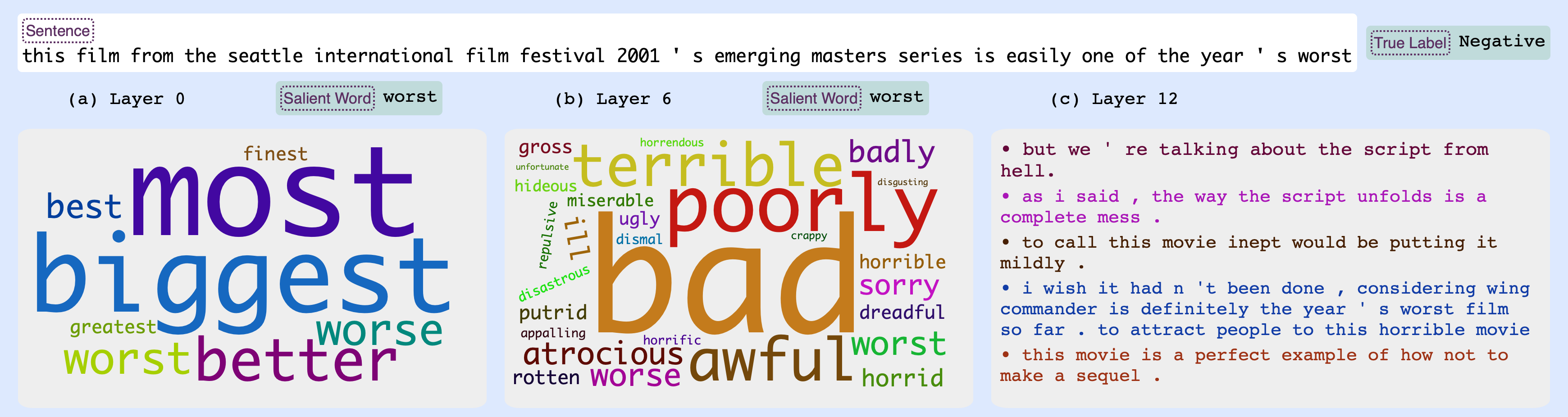
Figure 2: Sentiment task: Latent concepts of the most attributed words in Layers 0, 6 and 12

Data

We use Parts-of-Speech (POS) Tagging and Sentiment Classification (Sentiment) tasks for our experiments. The former is a sequence labeling task, where every word in the input sentence is assigned a POS tag, while the latter classifies sentences into two classes representing Positive and Negative sentiment. We use the Penn TreeBank dataset Marcus et al. (1993) for POS and the ERASER Movie Reviews dataset Pang and Lee (2004); Zaidan and Eisner (2008) for Sentiment. The POS dataset consists of 36k, 1.8k and 1.9k splits for train, dev and test respectively and 44 classes.

The ERASER movie review dataset consists of labeled paragraphs with human annotations of the words and phrases. We filter sentences that have a word/phrase labeled with sentiment and create a sentence-level sentiment classification dataset. The dataset consists of 9.4k positive and 8.6k negative instances. We randomly split it into 13k, 1.5k and 2.7k splits for train, dev and test respectively.

Models

We fine-tune 12-layered pre-trained models; BERT-base-cased Devlin et al. (2019), RoBERTa-base Liu et al. (2019) and XLM-Roberta Conneau et al. (2020) using the training datasets of the tasks. We use transformers Wolf et al. (2020) with the default settings and hyperparameters. Task-wise performance of the models is provided in Appendix Tables 4 and  5.

Module-specific hyperparameters

When extracting the activation and/or attribution of a word, we average the respective value over the word’s subword units. We optimize the number of clusters $K$ for each dataset as suggested by Dalvi et al. (2022). We use $K=600$ (POS) and $K=400$ (Sentiment) for ConceptDiscoverer.

Since the number of words in $\mathbb{D}$ can be very high, and the clustering algorithm is limited by the number of representations it can efficiently cluster, we filter out words with frequencies less than 5 and randomly select 20 contextual occurrences of every word with the assumption that a word may have a maximum of 20 facets. These settings are in line with Dalvi et al. (2022). In the case of [CLS] tokens, we keep all of the instances.

We use a zero-vector as the baseline vector in PredictionAttributor’s IG, using 500 approximation steps. For ConceptMapper, we use the cross-entropy loss with L2 regularization and train the classifier with ‘lbfgs’ solver and 100 maximum iterations. To optimize the classifier and to evaluate its performance, we split the dataset $\mathcal{D}$ into train ($90\%$) and test ($10\%$). ConceptMapper used in the LACOAT pipeline is trained using the full dataset $\mathcal{D}$. Finally, for PlausiFyer, we use ChatGPT with a temperature of 0 and a top_p value of 0.95.

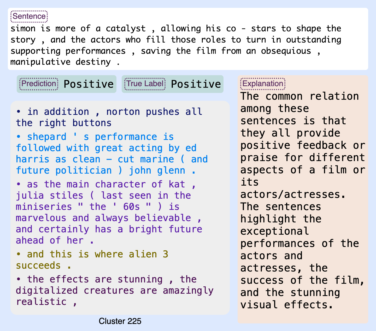
(a) Sentiment: A positive labeled test instance correctly predicted by the model.

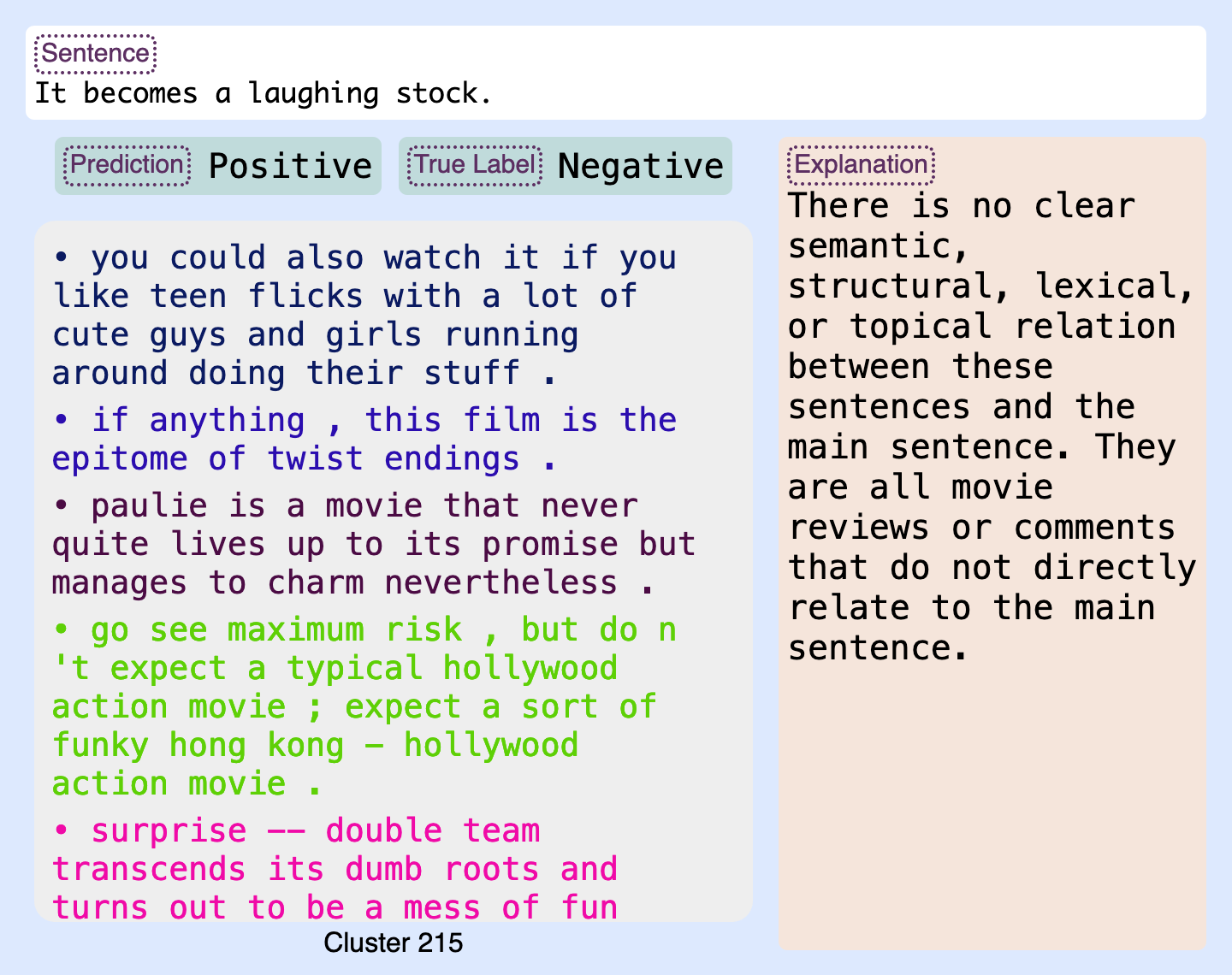
(b) Sentiment: A negatively labeled test instance that is incorrectly predicted as positive.

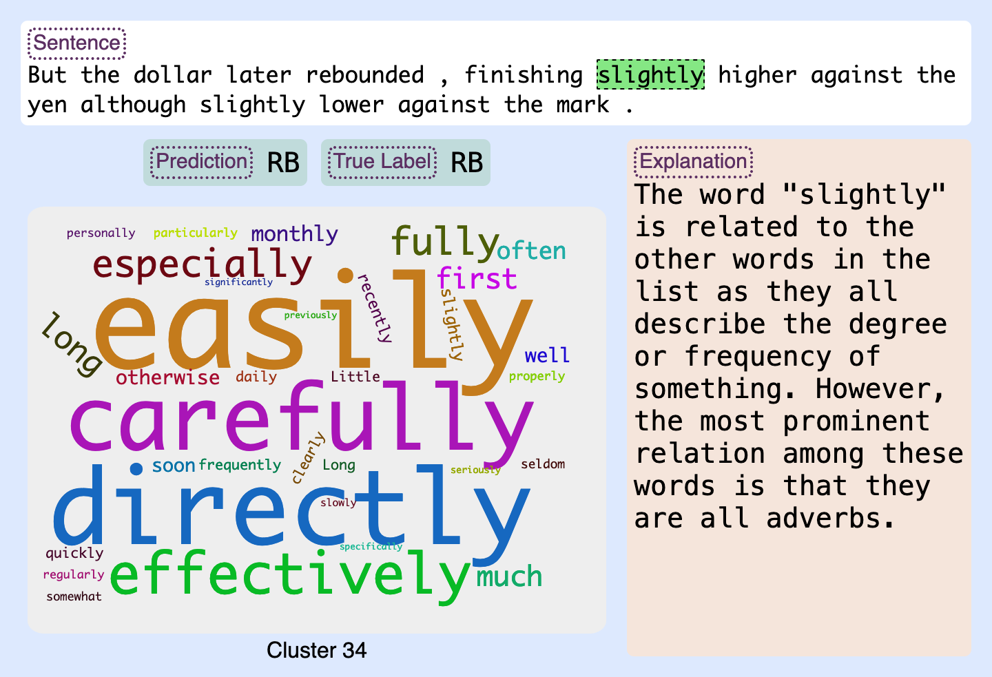
(c) POS: An adverb with semantics showing degree and intensity of an action

(d) POS: An incorrect prediction that can be detected from the latent concept

Figure 3: A few examples of LACOAT explanations for BERT using POS and Sentiment tasks

4 Evaluation

We perform a qualitative evaluation, a human evaluation and a module-level evaluation of LACOAT to measure its correctness and efficacy.

4.1 Qualitative Evaluation

In this section, we qualitatively evaluate the usefulness of the latent concept-based explanation and the generated human-friendly explanation.

4.1.1 Evolution of Concepts

LACOAT generates the explanation for each layer with respect to a prediction. The layer-wise explanation shows the evolution of concepts in making the prediction. Figure 2 shows layers 0, 6 and 12’s latent concept of the most attributed input token for RoBERTa fine-tuned on the sentiment task (see App Fig 5 for other examples). We found that the initial layer latent concepts do not always align with the sentiment of the input instance and may represent a general language concept. For instance, Figure 2(a) shows the concept of comparative and superlative adjectives of both positive and negative sentiments and is not limited to representing the negative sentiment of the most attributed word. In the middle layers, the latent concepts evolved into concepts that align better with the sentiment of the input sentence as can be seen in Figure 2(b). For instance, the latent concept of Figure 2(b) shows a mix of adjectives and adverbs of negative sentiment, i.e. aligned with the sentiment of the input sentence. In the sentiment task, the most attributed word in the last layer is [CLS] which resulted in latent concepts consisting of [CLS] representations of the most related sentences to the input. In such cases, we randomly pick five [CLS] instances from the latent concept and show their corresponding sentences in the figure (see Figure 2(c)). We found that the last layer’s latent concepts are best aligned with the input instance and its prediction and are the most informative explanation of the prediction. In the rest of the paper, we focus our analysis on the explanations generated using the last layer only and perform a human evaluation to evaluate their efficacy and correctness.

4.1.2 Analyzing Last Layer Explanations

Figure 3 presents various examples of LACOAT for both POS tagging and Sentiment tasks using BERT. The sentence is the input sentence, prediction is the output of the model and true label is the gold label. The explanation is the final output of LACOAT. Cluster X is the latent concept aligned with the most salient word representation at the 12th layer and X is the cluster ID. For sentiment, we randomly pick five [CLS] instances from the latent concept and show their corresponding sentences in the figure.

Correct prediction with correct gold label

Figures 3(a) and 3(c) present a case of correct prediction with latent-concept explanation and human-friendly explanation. The former are harder to interpret especially in the case of sentence-level latent concepts as in Figure 3(a) compared to latent concepts consisting of words (Figure 3(c)). However, in both cases, PlausiFyer highlights additional information about the relation between the latent concept and the input sentence. For example, it captures that the adverbs in Figure 3(c) have common semantics of showing degree or frequency. Similarly, it highlights that the reason of positive sentiment in 3(a) is due to praising different aspects of a film and its actors and actresses.

Wrong prediction with correct gold label

Figures 3(b) and 3(d) show rather interesting scenarios where the predicted label is wrong. In Figure 3(b), the input sentence has a negative sentiment but the model predicted it as positive. The instances of latent concepts show sentences with mixed sentiments such as “manages to charm” and “epitome of twist endings” is positive, and “never quite lives up to its promise” is negative. This provides the domain expert an evidence of a possible wrong prediction. The PlausiFyer’s explanation is even more helpful as it clearly states that “there is no clear … relation between these sentences …". Similarly, in the case of POS (Figures 3(d)) while the prediction is Noun, the majority of words in the latent concepts are plural Nouns, giving evidence of a possibly wrong prediction. In addition, the explanation did not capture any morphological relationship between the concept and the input word.

To study how the explanation would change if it is a correct prediction, we employ TextAttack Morris et al. (2020) to create an adversarial example of the sentence in Figure 3(b) that flips its prediction. The new sentence replaces “laughing” with “kidding” which has a similar meaning but flipped the prediction to a correct prediction. Figure 6 in the appendix shows the full explanation of the augmented sentence. With the correct prediction, the latent concept changed and the explanation clearly expresses a negative sentiment “… all express negative opinions and criticisms …" compared to the explanation of the wrongly predicted sentence.

Cross model analysis

LACOAT provides an opportunity to compare various models in terms of how they learned and structured the knowledge of a task. Figure 4 compares the explanation of RoBERTa (top) and XLMR (bottom) for identical inputs. Both models predicted the correct label. However, their latent concept based explanation is substantially different. RoBERTa’s explanation shows a large and diverse concept where many words are related to finance and economics. The XLMR’s latent concept is rather a small focused concept where the majority of tokens are units of measurement. It is worth noting that both models are fine-tuned on identical data.

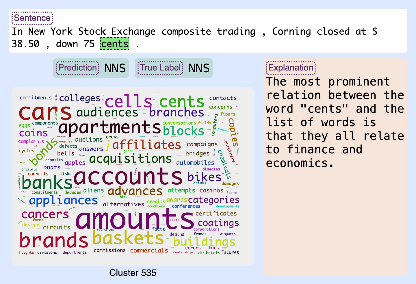
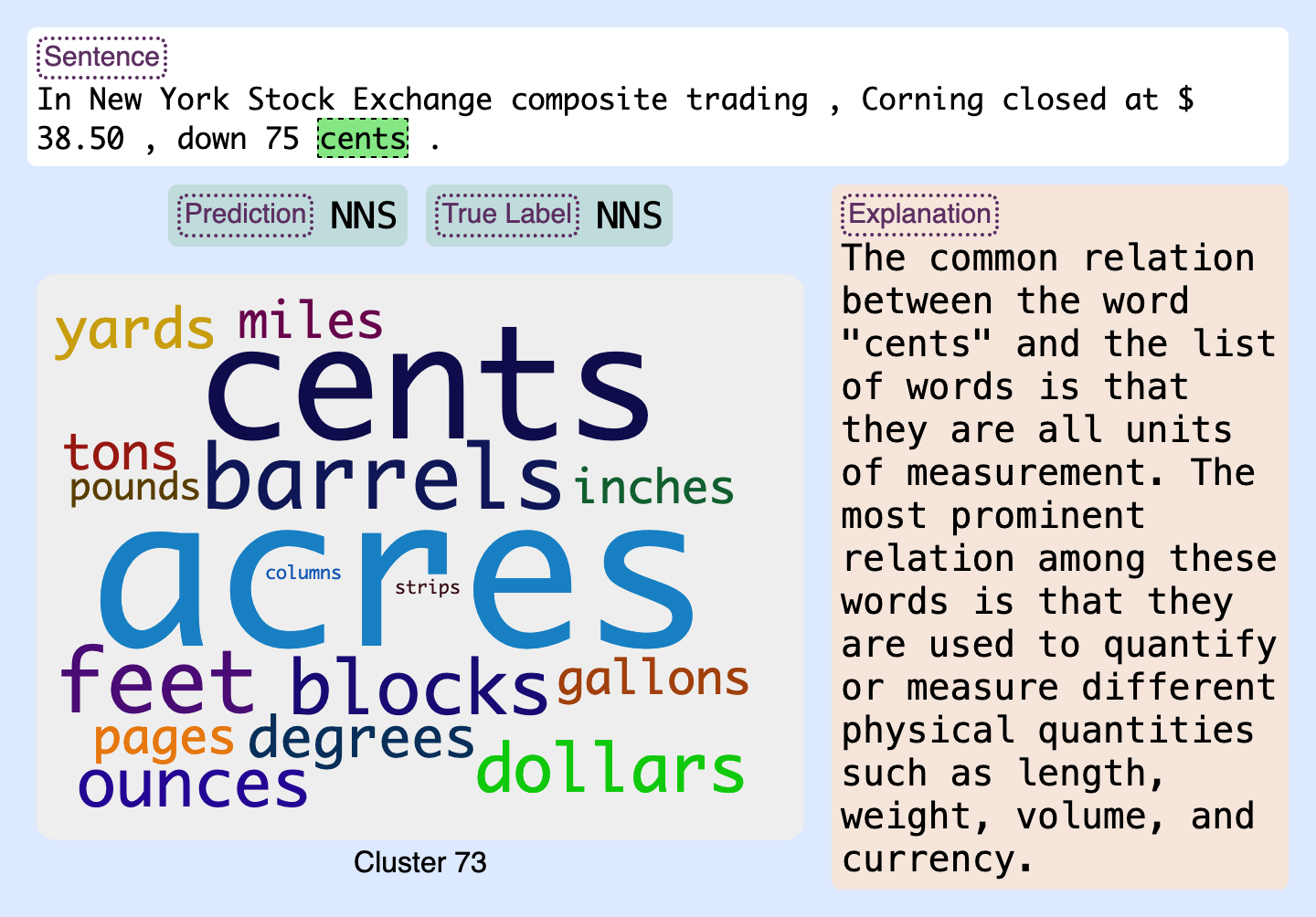
Figure 4: Comparing explanation of RoBERTa (top) and XLMR (bottom)

4.1.3 Comparison to Input Feature based Explanation

In Figure 2, layer 0 serves as a direct comparison to the explanation provided by the attribution methods. Here, IG highlights the input word “worst" in the given example. While it informs the user of the most salient input token that effects the prediction, it does not provide insights into the particular facet the model has used in that particular example. Even if we compare the explanation of other layers like layer 6, the latent concept of the attributed word is more informative than the attributed word alone.

4.2 Human Evaluation

To evaluate the explanation generated by LACOAT empirically, we conduct a human evaluation using four annotators across 50 test samples. Specifically, given an explanation (e.g. Figure 3), three annotators are asked to answer the following five questions:

1. Regardless of the prediction, can you see any relation between the original input and the concept used by the model? (Yes/No)

2. Given the prediction, does the latent concept help you understand why the model made that prediction? (Helps/Neutral/Hinders)

3. Given the prediction, does the explanation help you understand why the model made that prediction? (Helps/Neutral/Hinders)

4. Does the explanation accurately describe the latent concept? (Yes/No)

5. Is the explanation relevant to the task at hand? (Yes/No)

Q1 evaluates whether LACOAT attributes the correct concept to a given prediction, while Q2 and Q3 measure the efficacy of LACOAT’s output in helping a user understand the prediction. Q4 and Q5 evaluates the output of PlausiFyer. They specifically separate out the cases where the explanation was accurate but irrelevant to the task at hand.

Table 1 shows the consolidated labels by picking the majority label in case of Yes/No questions and averaging the annotations in case of the rest. The evaluation shows that the latent concept itself was not only relevant to the task at hand, but also helped the user understand the model’s prediction. The results for the helpfulness of the explanation text were mixed, with the majority of the annotations stating that it did not help or hinder their process. However upon inspection, we see that the explanation was mostly helpful in all the cases where the model made the correct prediction, and not helpful when the prediction was incorrect. Qualitatively analyzing the explanation text for incorrect prediction shows that PlausiFyer mostly outputs “There is no relationship between the sentences and the concepts”, which was deemed as hindering by most of the annotators. While such an explanation may serve as an indicator of a potential problem in the prediction, improving the prompt may result in a response that is indicative of the issue with the prediction. We leave this exploration for the future. Table 1 also shows the agreement between the annotators using Fleiss’ Kappa. Since not all samples were annotated by all annotators, we compute the average Fleiss’ kappa of each annotator with the consolidated annotation. The agreement ranges from Fair to Substantial across the five questions.

	Labels	Correct Samples	Incorrect Samples	All Samples
				Annotation	Fleiss $\kappa$
Q1	Yes/No	28 / 0	20 / 2	48 / 2	0.35
Q2	Helps/Neutral/Hinders	27 / 1 / 0	17 / 5 / 0	44 / 6 / 0	0.41
Q3	Helps/Neutral/Hinders	16 / 10 / 2	1 / 19 / 2	17 / 29 / 4	0.61
Q4	Yes/No	17 / 11	5 / 17	22 / 28	0.47
Q5	Yes/No	17 / 11	6 / 16	23 / 27	0.80

Table 1: Consolidated label distribution for Q1-Q5. Fleiss’ $\kappa$ scores are computed by averaging each annotator with the consolidated annotation. The consolidated labels and agreement scores are shown for all the samples, as well as partitioned into those where the model prediction was correct/incorrect.

4.3 Module Specific Evaluation

	POS		Sentiment
Layers	BERT	RoBERTa	BERT	RoBERTa
9	92.38	86.97	31.94	99.59
10	92.79	89.64	99.57	99.69
11	93.39	89.95	99.71	99.48
12	93.95	90.04	99.25	99.27

Table 2: Accuracy of PredictionAttributor in mapping a representation to the correct latent concept. See Appendix Table 7, 8, 9 for complete results.

The correctness of LACOAT depends on the performance of each module it comprised off. The ideal way to evaluate the efficacy of these modules is to consider gold annotations. However, they are not available for any module. To mitigate this limitation, we design various constrained scenarios where certain assumptions can be made about the representations of the model. For example, the POS model optimizes POS tags so it is highly probable that the last layer representations form latent concepts that are a good representation of POS tags as suggested by various previous works Kovaleva et al. (2019); Durrani et al. (2022). One can assume that for ConceptDiscoverer, the last layer latent concepts will form groupings of words based on specific tags and for PredictionAttributor, the input word at the position of the predicted tag should reside in a latent concept that is dominated by the words with the same tag. In the following, we evaluate the correctness of these assumptions.

Latent Concept Annotation For the sake of evaluation, we annotated the latent concepts automatically using the class labels of each task. Given a latent concept, we annotate it with a certain class if more than 90% of the words in the latent concept belong to that class. In the case of POS, the latent concepts will be labeled with one of the 44 tags. For sentiment, the class labels, Positive and Negative, are at sentence level. We tag a latent concept as Positive/Negative if 90% of its tokens ([CLS] or words) belong to sentences labeled as Positive/Negative in the training data. The latent concepts that do not fulfill the criteria of 90% for any class are annotated as Mixed.

4.3.1 ConceptDiscoverer

ConceptDiscoverer identifies latent concepts by clustering the representation. We questioned whether the discovered latent concepts are a true reflection of the properties that a representation possesses. Using ConceptDiscoverer, we form latent concepts of the last layer and automatically annotate them as described above. We found 87%, 83% and 86% of the latent concepts of BERT, RoBERTa and XLMR that perfectly map to a POS tag respectively. We further analyzed other concepts where 90% of the words did not belong to a single tag. We found them to be of compositional nature i.e. a concept consisting of related semantics like a mix of adjectives and proper nouns about countries such as Swedish and Sweden (Appendix Figure 9). For sentiment, we found 78%, 95% and 94% of the latent concepts of BERT, RoBERTa and XLMR to consist of either Positive or Negative sentences. The high number of class-based clusters of RoBERTa and XLMR show that at 12th layer, majority of their latent space is separated based on these two classes (see Table 6 for detailed results).

Layers		0	2	5	10	12
POS	Top 1	100	100	99.03	92.67	84.19
	Top 2	100	100	99.75	97.89	94.15
	Top 5	100	100	99.94	99.68	99.05
Sentiment	Top 1	100	100	97.19	83.09	68.24
	Top 2	100	100	99.63	92.67	83.24
	Top 5	100	100	99.94	97.75	94.24

Table 3: BERT: Accuracy of ConceptMapper in mapping a representation to the correct latent concept. See Table 10, 11 in the Appendix for results on all layers.

4.3.2 PredictionAttributor

We questioned whether the salient input representation correctly represents the latent space of the output. This specifically evaluates PredictionAttributor. We calculate the number of times the representation of the most salient word/[CLS] token maps to the latent concept of the identical label as that of the prediction. We expect a high alignment at the top layers for PredictionAttributor to be correct. We do not include ConceptMapper when evaluating this and conduct the experiment using the training data only where we already know the alignment of a salient representation and the latent concept. Table 2 shows the results across the last four layers (See Appendix Tables 7, 8, 9 for full results). For POS, we observed a successful match of 93.95%, 90.04% and 93.13% for BERT, RoBERTa and XLMR respectively. We observed the mismatched cases and found them to be also of a compositional nature i.e. latent concepts comprised of semantically related words (see Appendix Figure 9 for examples).

For sentiment, more than 99% of the time, the last layer’s salient representation maps to the predicted class label, confirming the correctness of PredictionAttributor. The performance drop for the lower layer is due to the absence of class-based latent concepts in the lower layers i.e. concepts that comprised more than 90% of the tokens belonging to sentences of one of the classes.

4.3.3 ConceptMapper

Here, we evaluate the correctness of ConceptMapper in mapping a test representation to the training data latent concepts. ConceptMapper trains using representations and their cluster ids as labels. For every layer, we randomly split this training data into 90% train and 10% test data. Here, the test data serves as the gold standard annotation of latent concepts. We train ConceptMapper using the training instances and measure the accuracy of the test instances. Table 3 presents the accuracy of the POS and Sentiment tasks using BERT (See Appendix Tables 10, 11 for results of other models). Observing Top-1 accuracy, the performance of ConceptMapper starts high (100%) for lower layers and drops to 84.19 and 68.24% for the last layer. We found that the latent space becomes dense on the last layer. This is in line with Ethayarajh (2019) who showed that the representations of higher layers are highly anisotropic. This causes several similar concepts close in the space. If true, the correct label should be among the top predictions of the mapper. We empirically tested it by considering the top two and top five predictions of the mapper, achieving a performance of up to 99.05% and 94.24% for the POS and Sentiment tasks respectively.

5 Related work

The explainability methods can be approached by local explanations and global explanations Madsen et al. (2023); Sundararajan et al. (2017a); Denil et al. (2014); Selvaraju et al. (2020); Kapishnikov et al. (2021); Zhao and Aletras (2023); Kim et al. (2018); Ghorbani et al. (2019); Jourdan et al. (2023); Zhao et al. (2023); Ribeiro et al. (2016). Lyu et al. (2023) provides a comprehensive survey on explainability methods in NLP. LACOAT is a local explanation method providing post-hoc explanations given an input instance. One of the most common ways for local explanations is to interpret the model prediction based on the input features. However, the shortcoming of such an explanation is the lack of contextual verbosity, which could not interpret the multifaceted roles of the input features.

A number of works attempted to explain and interpret NLP models using human-defined concepts Kim et al. (2018) and concepts extracted from hidden representations Zhao et al. (2023); Ghorbani et al. (2019); Rajani et al. (2020). Zhao et al. (2023); Kim et al. (2018) worked on the global explanation based on a surrogate model. Zhao et al. (2023) trained the surrogate model using on two optimization criteria i.e. auto encoding loss to stay faithful to the original model distribution and impact of the latent concept to prediction. Different from them, we provide local explanations and we ensure the faithfulness of latent concepts to the model by extracting them directly from the hidden representation without any supervised training. Rajani et al. (2020) used k-nearest neighbors of the training data for low-confidence predictions and showed them to be useful in revealing erroneous correlations and misclassified instances and enhancing the performance of the finetuned model.  Dalvi et al. (2022) analyzed latent concepts of pretrained models in terms of their ability to represent linguistic knowledge. Our ConceptDiscoverer module is motivated from them. However, we propose a method to explain a model’s prediction using training data latent concepts.

6 Conclusion

We presented LACOAT that provides a human-friendly explanation of a model’s prediction. The qualitative evaluation and human evaluation showed that LACOAT explanations are insightful in explaining a correct prediction, in highlighting a wrong prediction and in comparing the explanations of models. The reliance on training data latent space enables interpreting how knowledge is structured in the network. Similarly, it enables the study of the evolution of predictions across layers. LACOAT promises human-in-the-loop in the decision-making process and is a step towards trust in AI.

7 Limitations

A few limitations of LACOAT are: 1) while hierarchical clustering is better than nearest neighbor in discovering latent concepts as established by Dalvi et al. (2022), it has computational limitations and it can not be easily extended to a corpus of say 1M tokens. However, the assumptions that are taken in the experimental setup e.g. considering the maximum 20 occurrences of a word (supported by Dalvi et al. (2022)) work well in practice in terms of limiting the number of tokens and covering all facets of a majority of the words. Moreover, the majority of the real-world tasks have limited task-specific data and LACOAT can effectively be applied in such cases.

2) LACOAT requires white-box access to the training data and the model for explanation which may not be available for large language models such as Llama and ChatGPT. For open-source models like Llama and Mistral, LACOAT can be applied in their task-specific usage. For instance for sentiment classification using Llama, the training data of sentiment can be used to extract the latent space of Llama for the sentiment classification task. However, the applicability of LACOAT for generative tasks is limited due to the open vocabulary.

Appendix A Salient Representation Extraction - Position Based Attribution Method

This strategy uses the position of the output head as an indication of the most salient contextual representation. For instance,

• In the case of sequence classification, the representation of the [CLS] token, $\overrightarrow{z}_{\texttt{[CLS]}}$ (or a model’s representative classification token) will be considered as the most salient representation.

• In the case of masked token prediction, the representation of the [MASK] token ($\overrightarrow{z}_{\texttt{MASK}}$) will be considered as the most salient for making the prediction.

• In the case of sequence labeling, the representation at the time step of the prediction will be used. For example, in the case of POS tagging, for the prediction of a tag of the word love in the sentence I [love] soccer, the second time step’s representations ($\overrightarrow{z}_{w_{2}}$) will be used.

Appendix B Finetuning Performance

We tuned several transformers BERT-base-cased, RoBERTa and XLM-RoBERTa. We used standard splits for training, development and test data that we used to carry out our analysis. The splits to preprocess the data are available through git repository. See Table 4 and Table 5 for statistics and classifier accuracy.

Task	Train	Dev	Test	Tags	BERT	RoBERTa	XLM-R
POS	36557	1802	1963	48	96.81	96.70	96.75

Table 4: The fine-tuned performance of models, data statistics (number of sentences) on training, development, and test sets used in the experiments, and the number of tags to be predicted for the POS tagging task. Model: BERT, RoBERTa, XLM-R

Task	Train	Dev	Test	Tags	BERT	RoBERTa	XLM-R
Sentiment	13878	1516	2726	2	94.53	96.31	93.80

Table 5: The fine-tuned performance of models, data statistics (number of sentences) on training, development, and test sets used in the experiments, and the number of tags to be predicted for the sentiment classification task. Model: BERT, RoBERTa, XLM-R

Appendix C Qualitative Evaluation - More Examples

C.1 Example for the Evolution of Concepts

5 presents the other example of latent concepts of the salient words in layer 0, 6, and 12. Similarly to the example shown in 2, the latent concept of this example shows that the different forms of the verb “sit” and are not aligned with its usage in the input instance. The concept in the middle layer aligns better with the sentiment of the input sentence(Figure 5(b)). The most words of layer 6’s latent concept match the sentiment of the input sentence. We also randomly pick five [CLS] instances from the latent concept and show their corresponding sentences in the figure (see Figure 5(c)). The concept of the last layer is best aligned with the input sentence.

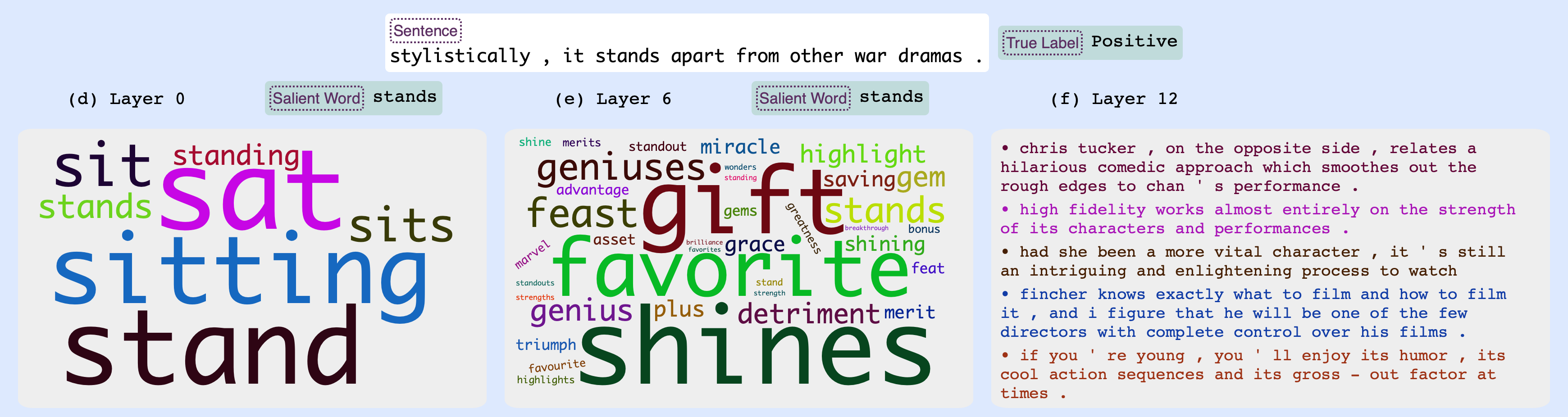
Figure 5: Sentiment task: Examples of the latent concepts of the most attributed words in Layers 0, 6 and 12

C.2 Adversarial Example of the Sentence in Figure 3(b)

The augmented sentence has a similar meaning word “kidding” instead of “laughing” (See Figure 6). The predicted label of the sentence becomes Positive, which is matched to the gold label. The latent concept of the “kidding” is more aligned with the sentence than the original one.

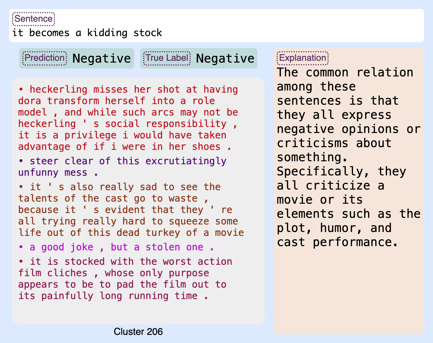
Figure 6: An augmented example for the test instance in Figures 3(b): The augmented sentence replaced the “laughing” with “kidding” which has a similar meaning. The label of the augmented sentence becomes positive, which is matched with the gold label. The new predicted latent concept is more closely aligned with the main sentence. The model may not learn the implicit meaning of the “laughing stock” in the sentence.

C.3 Correct Predicted Label with Incorrect Gold Label

The automatic labeling of latent concepts based on the model’s class provides an opportunity to analyze the wrong predictions of the model with respect to the concept labels. We specifically observe the wrong predictions of test instances. We discovered that many of the wrong prediction cases were not caused by misclassification of the models but were due to the fact that the gold label was annotated incorrectly. Figure 7 shows an example in which the main sentence and the explanation sentence share the same sentiment. We can see that the sentence provides critiques of the different aspects of the film. But the gold label of this sentence is positive. We think the gold label for this sentence is incorrect.

Figure 7: A correct prediction but incorrect gold label: The test instance emphasizes the movie’s shortcomings and uses the word "especially" to highlight the flaws. The explanation is rather long but it correctly highlights that the sentences are about “critiques or opinions"

C.4 Incorrect Prediction in POS tagging Task

Figure 8 presents an incorrect prediction in the POS tagging task. The prediction is aligned with a mixed concept that consists of nouns and adjectives. According to the latent concept explanation, we know that the model may not learn to distinguish the “noun” and “adjective”, which causes the incorrect prediction.

Figure 8: An incorrect prediction (noun vs adjective) based on a latent concept made up of a mixture of nouns and adjectives: the “deputy” in this case is an adjective. The prediction aligns with a mixed cluster that contains both nouns and adjectives and the model may not learn to distinguish the “noun” and “adjective” in this case. The latent concept explanation is useful for the user to know that the model has used a mixed latent space for the prediction. The Explanation is rather wrong since it mentions that all these words are nouns.

	Sentiment
	BERT			RoBERTa			XLM-R
Layer	Neg	Pos	Mix	Neg	Pos	Mix	Neg	Pos	Mix
Layer 0	49	1	350	45	0	355	55	0	345
Layer 1	53	1	346	50	0	350	58	0	342
Layer 2	51	1	348	49	0	351	62	0	338
Layer 3	53	0	347	60	0	340	62	0	338
Layer 4	57	0	343	52	0	348	69	0	331
Layer 5	56	0	344	51	0	349	68	0	332
Layer 6	57	0	343	45	1	354	59	1	340
Layer 7	51	0	349	56	2	342	68	0	332
Layer 8	49	0	351	116	25	259	71	0	329
Layer 9	66	4	330	226	126	48	82	7	311
Layer 10	125	31	244	235	140	25	257	92	51
Layer 11	174	49	177	258	120	22	256	110	34
Layer 12	230	81	89	254	126	20	105	270	25

Table 6: Number of clusters for each polarity: “Neg” for negative Label, “Pos” for positive, and “Mix” for mix label. The total number of clusters is 400.

Appendix D Module Specific Evaluation

D.1 ConceptDiscoverer - Compositional Concept Examples

We found that the concepts are not always formed aligning to the output class. Some concepts are formed by combining words from different classes. For example in Figure 9(a), the concept is composed of nouns (specifically countries) and adjectives that modify these country nouns. Similarly, Figure 9(b) describes a concept composed of different forms of verbs.

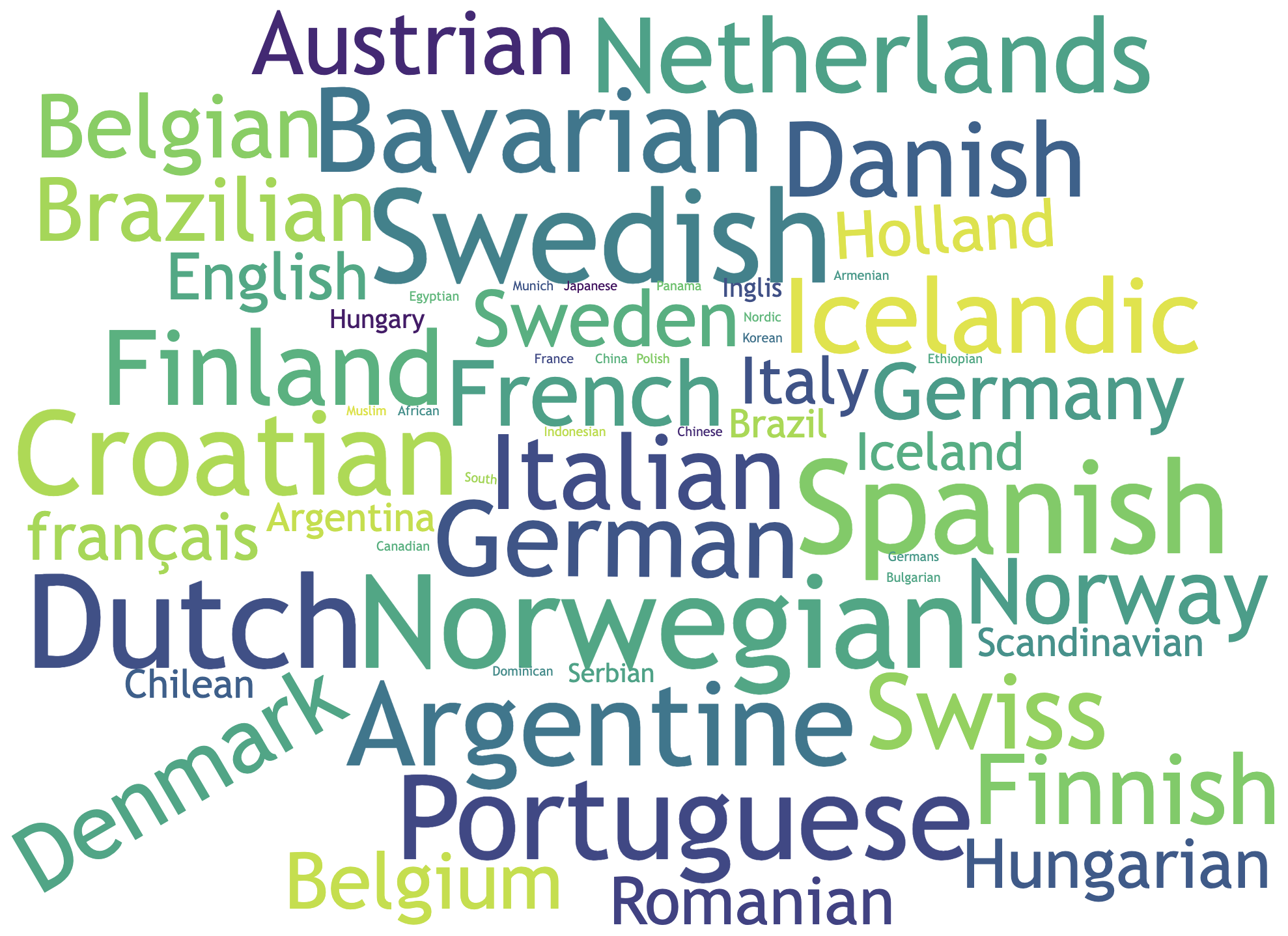
(a)

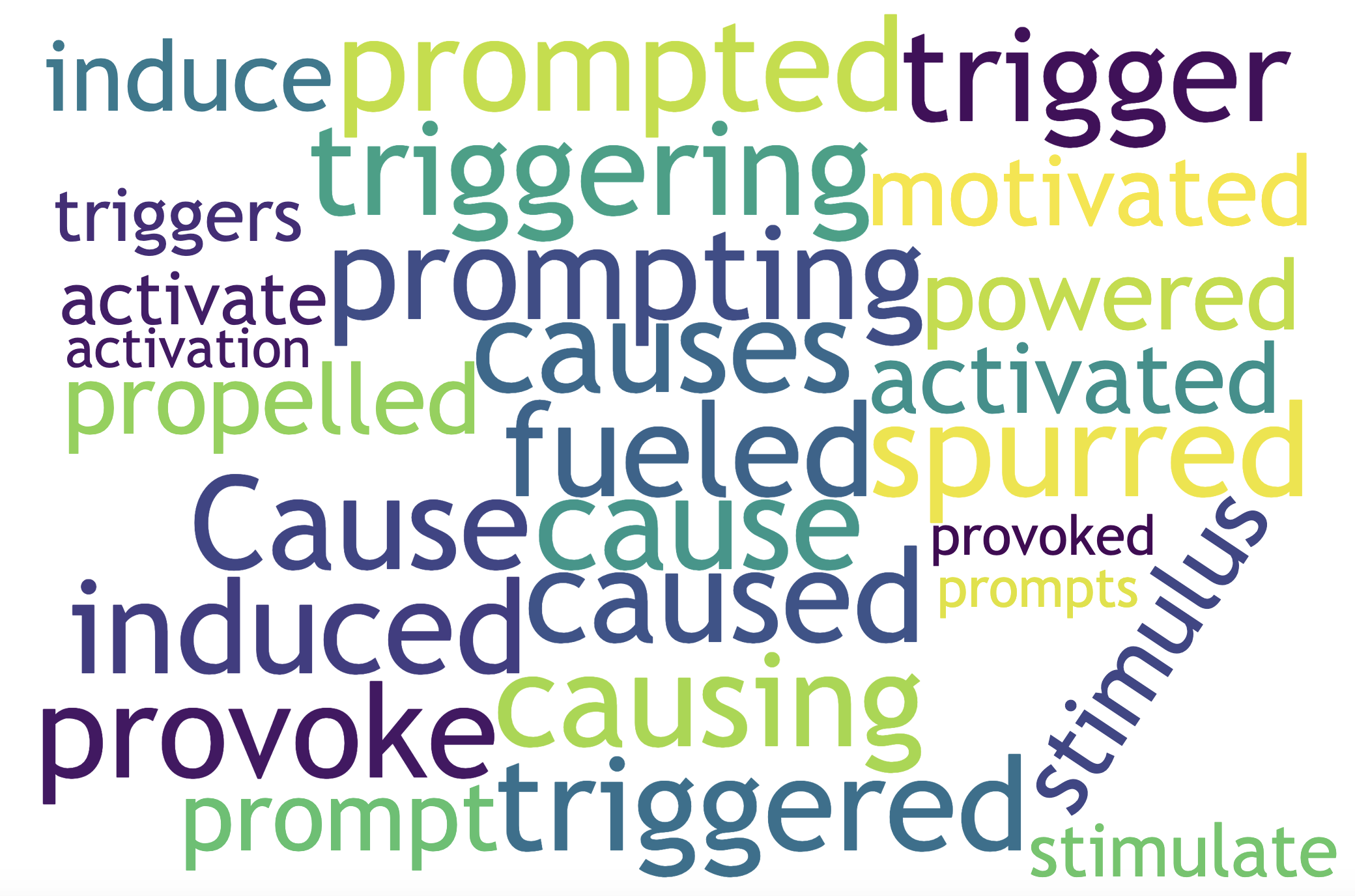
(b)

Figure 9: Compositional concepts: (a) A cluster representing countries (NNP) and their adjectives (JJ), (b) Different form of verbs (Gerunds, Present and Past participles).

D.2 ConceptDiscoverer - Number of Clusters For Each Polarity in the Sentiment Classification Task

Table 6 provides the number of clusters for each polarity in the sentiment classification task. It shows that the majority of latent concepts are class-based clusters at the last layer for the BERT, RoBERTa, and XLMR models.

D.3 ConceptMapper - Position Based Attribution Method

We evaluate the module that is based on the position based attribution approach as the number of times an input representation at the position of the output head maps to the latent concept that is annotated with an identical label as the output. For example, consider that the model predicts Proper Noun (PN) for the input word "Trump". In order for the input representation of the predicted label to be aligned with the latent concept, the representation of the word "Trump" on at least the last layer should be in a cluster of words whose label is PN. Similarly for sentiment classification, we expect the [CLS] representation on the last layer to map to a latent concept that is dominated by the same class as the prediction.

For POS tagging task, the salient representation is identical for both the position based and saliency based methods and results in the same performance (Table 7). For the sentiment classification task, performance drops and even reaches zero as in the case of XLMR. This may be due to the position-based method which fails to find the right latent concept when the most attributed word is different from the position of the output head (Table 8).

	POS
Layer	BERT	RoBERTa	XLM-R
Layer 0	16.81	14.29	17.66
Layer 1	17.79	16.49	18.89
Layer 2	21.16	20.18	20.71
Layer 3	22.79	20.13	31.03
Layer 4	29.70	24.65	40.51
Layer 5	46.74	29.26	60.31
Layer 6	73.19	42.38	77.32
Layer 7	84.52	57.46	85.78
Layer 8	90.68	82.84	89.41
Layer 9	92.38	86.97	91.97
Layer 10	92.79	89.64	92.64
Layer 11	93.39	89.95	92.59
Layer 12	93.95	90.04	93.13

Table 7: Position/Saliency-based method: accuracy of PredictionAttributor in mapping a representation to the correct latent concept in the POS tagging task.

	Sentiment
Layer	BERT	RoBERTa	XLM-R
Layer 0	0	0	0
Layer 1	0	0	0
Layer 2	0	0	0
Layer 3	0	0	0
Layer 4	0	0	0
Layer 5	0	0	0
Layer 6	0	0	0
Layer 7	0	0	0
Layer 8	0	99.11	0
Layer 9	37.09	98.45	0
Layer 10	99.55	99.14	0
Layer 11	99.82	99.27	99.17
Layer 12	99.25	99.27	99.08

Table 8: Position-based method: accuracy of PredictionAttributor in mapping a representation to the correct latent concept in the Sentiment Classification task. The reason of zero values is that the position-based method fails to find the right latent concept when the most attributed word is different from the position of the output head.

	Sentiment
Layer	BERT	RoBERTa	XLM-R
Layer 0	6.40	12.08	7.46
Layer 1	7.12	12.46	5.57
Layer 2	7.66	17.29	6.36
Layer 3	7.13	22.00	8.03
Layer 4	12.18	20.08	9.71
Layer 5	13.24	24.25	8.88
Layer 6	11.18	17.26	8.75
Layer 7	12.80	39.87	14.05
Layer 8	4.06	92.84	15.75
Layer 9	31.94	99.59	32.63
Layer 10	99.57	99.69	92.06
Layer 11	99.71	99.48	94.97
Layer 12	99.25	99.27	99.08

Table 9: Saliency-based method: accuracy of PredictionAttributor in mapping a representation to the correct latent concept in the sentiment classification task. The reason of very low values for the lower layers is mainly due to the absence of class-based latent concepts in the lower layers i.e. concepts that comprised more than 90% of the tokens belonging to sentences of one of the classes.

D.4 ConceptMapper - Accuracy of ConceptMapper for the Sentiment Classification and POS Tagging task

We validate ConceptMapper by measuring the accuracy of the test instances for both the sentiment classification and POS tagging tasks based on the BERT, RoBERTa, and XLMR models. The top 1, 2, and 5 accuracy of ConceptMapper in mapping a representation to the correct latent concept for each layer is shown in Table 10 and Table 11. For all models, the performance of the top-5 is above 99% for the POS tagging task and above 90% for the sentiment classification task.

	POS
	BERT			RoBERTa			XLM-R
Layer	Top-1	Top-2	Top-5	Top-1	Top-2	Top-5	Top-1	Top-2	Top-5
Layer 0	100	100	100	99.91	99.95	99.98	99.99	100	100
Layer 1	100	100	100	99.92	99.94	99.98	100	100	100
Layer 2	100	100	100	99.76	99.92	99.98	99.72	99.98	100
Layer 3	99.85	99.98	100	99.38	99.85	99.98	98.25	99.60	99.98
Layer 4	99.72	99.92	99.97	98.67	99.58	99.87	97.72	99.60	99.98
Layer 5	99.03	99.75	99.94	97.69	99.15	99.73	97.05	99.23	99.91
Layer 6	97.76	99.34	99.83	96.52	98.71	99.59	95.8	98.95	99.76
Layer 7	96.51	98.91	99.68	94.72	98.11	99.57	93.92	98.31	99.80
Layer 8	95.27	98.52	99.79	92.56	97.55	99.52	94.20	98.52	99.80
Layer 9	94.54	98.25	99.70	92.24	97.48	99.55	92.79	97.82	99.73
Layer 10	92.67	97.89	99.68	91.61	97.19	99.55	92.03	97.66	99.60
Layer 11	90.86	97.34	99.64	90.72	96.77	99.58	90.40	97.28	99.67
Layer 12	84.19	94.15	99.05	86.88	95.13	99.15	85.07	94.57	99.08

Table 10: Top 1, 2, and 5 accuracy of  ConceptMapper in mapping a representation to the correct latent concept for the POS tagging task. The top-5 performance reaches above 99% for all models demonstrating that the correct latent concept is among the top probable latent concepts of ConceptMapper.

	Sentiment
	BERT			RoBERTa			XLM-R
Layer	Top-1	Top-2	Top-5	Top-1	Top-2	Top-5	Top-1	Top-2	Top-5
0	100	100	100	99.95	100	100	100	100	100
1	100	100	100	99.86	99.98	100	100	100	100
2	100	100	100	99.89	99.98	100	99.9	100	100
3	98.80	100	100	99.44	99.83	99.96	99.57	99.99	100
4	97.84	99.85	99.99	99.28	99.73	99.91	99.4	99.96	100
5	97.19	99.63	99.94	98.4	99.5	99.84	99.12	99.84	99.96
6	96.44	99.30	99.89	97.35	99.15	99.82	98.9	99.84	99.96
7	94.86	98.97	99.90	96.13	98.74	99.63	98.22	99.62	99.9
8	93.26	97.99	99.67	87.42	95.14	98.43	98.13	99.48	99.84
9	90.42	96.97	99.20	75.38	88.14	96.07	96.37	98.77	99.66
10	83.09	92.67	97.75	65.84	81.13	93.46	89.12	95.2	98.61
11	76.84	88.02	96.01	65.91	81.36	93.43	70.99	84.31	94.18
12	68.24	83.24	94.24	70.83	84.54	95.67	55.3	75.08	91.74

Table 11: Top 1, 2, and 5 accuracy of  ConceptMapper in mapping a representation to the correct latent concept for the sentiment classification task. The top-5 performance reaches above 90% for all models demonstrating that the correct latent concept is among the top probable latent concepts of ConceptMapper.

References

- Conneau et al. (2020) Alexis Conneau, Kartikay Khandelwal, Naman Goyal, Vishrav Chaudhary, Guillaume Wenzek, Francisco Guzmán, Edouard Grave, Myle Ott, Luke Zettlemoyer, and Veselin Stoyanov. 2020. Unsupervised cross-lingual representation learning at scale. In Proceedings of the 58th Annual Meeting of the Association for Computational Linguistics, pages 8440–8451. Association for Computational Linguistics.
- Dalvi et al. (2022) Fahim Dalvi, Abdul Rafae Khan, Firoj Alam, Nadir Durrani, Jia Xu, and Hassan Sajjad. 2022. Discovering latent concepts learned in BERT. In International Conference on Learning Representations.
- Denil et al. (2014) Misha Denil, Alban Demiraj, and Nando de Freitas. 2014. Extraction of salient sentences from labelled documents. CoRR, abs/1412.6815.
- Devlin et al. (2019) Jacob Devlin, Ming-Wei Chang, Kenton Lee, and Kristina Toutanova. 2019. BERT: Pre-training of deep bidirectional transformers for language understanding. In Proceedings of the 2019 Conference of the North American Chapter of the Association for Computational Linguistics: Human Language Technologies, NAACL-HLT ’19, pages 4171–4186, Minneapolis, Minnesota, USA. Association for Computational Linguistics.
- Durrani et al. (2022) Nadir Durrani, Hassan Sajjad, Fahim Dalvi, and Firoj Alam. 2022. On the transformation of latent space in fine-tuned NLP models. In Proceedings of the 2022 Conference on Empirical Methods in Natural Language Processing, pages 1495–1516, Abu Dhabi, United Arab Emirates. Association for Computational Linguistics.
- Ethayarajh (2019) Kawin Ethayarajh. 2019. How contextual are contextualized word representations? Comparing the geometry of BERT, ELMo, and GPT-2 embeddings. In Proceedings of the 2019 Conference on Empirical Methods in Natural Language Processing and the 9th International Joint Conference on Natural Language Processing (EMNLP-IJCNLP), pages 55–65, Hong Kong, China. Association for Computational Linguistics.
- Ghorbani et al. (2019) Amirata Ghorbani, James Wexler, James Zou, and Been Kim. 2019. Towards Automatic Concept-based Explanations. ArXiv:1902.03129 [cs, stat].
- Gowda and Krishna (1978) K Chidananda Gowda and G Krishna. 1978. Agglomerative clustering using the concept of mutual nearest neighbourhood. Pattern recognition, 10(2):105–112.
- Jourdan et al. (2023) Fanny Jourdan, Agustin Picard, Thomas Fel, Laurent Risser, Jean Michel Loubes, and Nicholas Asher. 2023. COCKATIEL: COntinuous Concept ranKed ATtribution with Interpretable ELements for explaining neural net classifiers on NLP tasks. ArXiv:2305.06754 [cs, stat].
- Kapishnikov et al. (2021) Andrei Kapishnikov, Subhashini Venugopalan, Besim Avci, Ben Wedin, Michael Terry, and Tolga Bolukbasi. 2021. Guided Integrated Gradients: An Adaptive Path Method for Removing Noise. ArXiv:2106.09788 [cs].
- Kim et al. (2018) Been Kim, Martin Wattenberg, Justin Gilmer, Carrie Cai, James Wexler, Fernanda Viegas, and Rory Sayres. 2018. Interpretability Beyond Feature Attribution: Quantitative Testing with Concept Activation Vectors (TCAV). ArXiv:1711.11279 [stat].
- Kovaleva et al. (2019) Olga Kovaleva, Alexey Romanov, Anna Rogers, and Anna Rumshisky. 2019. Revealing the dark secrets of BERT. In Proceedings of the 2019 Conference on Empirical Methods in Natural Language Processing and the 9th International Joint Conference on Natural Language Processing (EMNLP-IJCNLP), pages 4365–4374, Hong Kong, China. Association for Computational Linguistics.
- Liu et al. (2019) Yinhan Liu, Myle Ott, Naman Goyal, Jingfei Du, Mandar Joshi, Danqi Chen, Omer Levy, Mike Lewis, Luke Zettlemoyer, and Veselin Stoyanov. 2019. RoBERTa: A robustly optimized BERT pretraining approach. ArXiv:1907.11692.
- Lyu et al. (2023) Qing Lyu, Marianna Apidianaki, and Chris Callison-Burch. 2023. Towards Faithful Model Explanation in NLP: A Survey. ArXiv:2209.11326 [cs].
- Madsen et al. (2023) Andreas Madsen, Siva Reddy, and Sarath Chandar. 2023. Post-hoc Interpretability for Neural NLP: A Survey. ACM Computing Surveys, 55(8):1–42. ArXiv:2108.04840 [cs].
- Marcus et al. (1993) Mitchell P. Marcus, Beatrice Santorini, and Mary Ann Marcinkiewicz. 1993. Building a large annotated corpus of English: The Penn Treebank. Computational Linguistics, 19(2):313–330.
- Mikolov et al. (2013) Tomas Mikolov, Kai Chen, Greg Corrado, and Jeffrey Dean. 2013. Efficient estimation of word representations in vector space. In Proceedings of the ICLR Workshop, Scottsdale, AZ, USA.
- Morris et al. (2020) John Morris, Eli Lifland, Jin Yong Yoo, Jake Grigsby, Di Jin, and Yanjun Qi. 2020. Textattack: A framework for adversarial attacks, data augmentation, and adversarial training in nlp. In Proceedings of the 2020 Conference on Empirical Methods in Natural Language Processing: System Demonstrations, pages 119–126.
- Pang and Lee (2004) Bo Pang and Lillian Lee. 2004. A sentimental education: Sentiment analysis using subjectivity summarization based on minimum cuts. In Proceedings of the 42nd Annual Meeting on Association for Computational Linguistics, ACL ’04, page 271–es, USA. Association for Computational Linguistics.
- Rajani et al. (2020) Nazneen Fatema Rajani, Ben Krause, Wengpeng Yin, Tong Niu, Richard Socher, and Caiming Xiong. 2020. Explaining and improving model behavior with k nearest neighbor representations.
- Reif et al. (2019) Emily Reif, Ann Yuan, Martin Wattenberg, Fernanda B Viegas, Andy Coenen, Adam Pearce, and Been Kim. 2019. Visualizing and measuring the geometry of bert. In Advances in Neural Information Processing Systems, volume 32. Curran Associates, Inc.
- Ribeiro et al. (2016) Marco Ribeiro, Sameer Singh, and Carlos Guestrin. 2016. “why should I trust you?”: Explaining the predictions of any classifier. In Proceedings of the 2016 Conference of the North American Chapter of the Association for Computational Linguistics: Demonstrations, pages 97–101, San Diego, California. Association for Computational Linguistics.
- Selvaraju et al. (2020) Ramprasaath R. Selvaraju, Michael Cogswell, Abhishek Das, Ramakrishna Vedantam, Devi Parikh, and Dhruv Batra. 2020. Grad-CAM: Visual Explanations from Deep Networks via Gradient-based Localization. International Journal of Computer Vision, 128(2):336–359. ArXiv:1610.02391 [cs].
- Shrikumar et al. (2017) Avanti Shrikumar, Peyton Greenside, and Anshul Kundaje. 2017. Learning important features through propagating activation differences. In Proceedings of the 34th International Conference on Machine Learning - Volume 70, ICML’17, page 3145–3153. JMLR.org.
- Simonyan et al. (2014) Karen Simonyan, Andrea Vedaldi, and Andrew Zisserman. 2014. Deep inside convolutional networks: Visualising image classification models and saliency maps. In Workshop at International Conference on Learning Representations.
- Sundararajan et al. (2017a) Mukund Sundararajan, Ankur Taly, and Qiqi Yan. 2017a. Axiomatic Attribution for Deep Networks. ArXiv:1703.01365 [cs].
- Sundararajan et al. (2017b) Mukund Sundararajan, Ankur Taly, and Qiqi Yan. 2017b. Axiomatic attribution for deep networks. In Proceedings of the 34th International Conference on Machine Learning, volume 70 of Proceedings of Machine Learning Research, pages 3319–3328. PMLR.
- Wolf et al. (2020) Thomas Wolf, Lysandre Debut, Victor Sanh, Julien Chaumond, Clement Delangue, Anthony Moi, Pierric Cistac, Tim Rault, Rémi Louf, Morgan Funtowicz, Joe Davison, Sam Shleifer, Patrick von Platen, Clara Ma, Yacine Jernite, Julien Plu, Canwen Xu, Teven Le Scao, Sylvain Gugger, Mariama Drame, Quentin Lhoest, and Alexander M. Rush. 2020. Transformers: State-of-the-art natural language processing. In Proceedings of the 2020 Conference on Empirical Methods in Natural Language Processing: System Demonstrations, pages 38–45, Online. Association for Computational Linguistics.
- Zaidan and Eisner (2008) Omar Zaidan and Jason Eisner. 2008. Modeling annotators: A generative approach to learning from annotator rationales. In Proceedings of the 2008 Conference on Empirical Methods in Natural Language Processing, pages 31–40, Honolulu, Hawaii. Association for Computational Linguistics.
- Zhao et al. (2023) Ruochen Zhao, Shafiq Joty, Yongjie Wang, and Tan Wang. 2023. Explaining Language Models’ Predictions with High-Impact Concepts. ArXiv:2305.02160 [cs].
- Zhao and Aletras (2023) Zhixue Zhao and Nikolaos Aletras. 2023. Incorporating Attribution Importance for Improving Faithfulness Metrics. In Proceedings of the 61st Annual Meeting of the Association for Computational Linguistics (Volume 1: Long Papers), pages 4732–4745, Toronto, Canada. Association for Computational Linguistics.