Coil-to-globule collapse of active polymers: a Rouse perspective

Abstract

We derive an effective Rouse model for tangentially active polymers, characterized by a constant active force tangent to their backbone. In particular, we show that, once extended to account for finite bending rigidity, such active Rouse model captures the reduction in the gyration radius, or coil-to-globule-like transition, that has been observed numerically in the literature for such active filaments. Interestingly, our analysis identifies the proper definition of the Peclet number, that allows to collapse all numerical data onto a master curve.

1 Introduction

By means of breaking equilibrium at the local, microscopic scale, active systems show dynamical and collective properties that differ quite much from their equilibrium or even driven counterparts[1, 2]. For example, a collection of active Brownian colloids can undergo Motility Induced Phase Separation[3, 4] leading to the onset of big clusters even in the absence of any attractive interaction between the particles. Similarly, micro-phase separation has been observed in continuum models that mimic an active bath[5]. Besides MIPS, active systems present out-of-equilibrium phases such as living crystalline clusters [6, 7], active turbulence [8], self-assembly [9, 10] and various types of flocking phases [11, 12, 13].
Among active systems, those made of filamentous units have particular relevance in biological systems, example being the cytoskeleton[14] and the intracellular trafficking network[15], chromatin[16, 17, 18], cilia arrays[19, 20] and flagella[21] as well as micro-organisms[22, 23, 24]. At the macroscopic scale, worms collectives show interesting emerging properties[25]. More generally, technological progress in the synthesis of artificial active chains[26, 27, 28, 29] as well as chains of chemically active droplets[30, 31] and soft robotic systems[32, 33, 34] make active filaments ubiquitous and open up the possibility of a huge range of applications.
Inspired by these examples, focus has been recently put onto characterising the properties of active polymers, i.e. polymers made out of “active” monomers. In this context, activity can be realised in different ways[35]: by means of a temperature mismatch[36, 37, 38], correlated noise along the backbone[39, 17], completely random self-propulsion forces (or Active Brownian Polymer)[40, 41, 42, 43] or correlated forces, oriented either perpendicularly[44] or along the polymer backbone[45, 46]. In this manuscropt, we focus on the last case, as it is believed to mimic the action of molecular motors[47, 48] as well as the locomotive mechanism of worms [49, 25], that contract their segments or use lateral protrusions to crawl or swim forward.
Notably, the way in which a tangential force can be realized is not unique. Indeed, one can choose to consider a propulsion force (i) constant in magnitude and parallel to the local backbone tangent[46, 50, 51, 52, 53, 23, 54, 55, 56]; (ii) constant in magnitude and parallel to the bond between neighbours along the chain[57, 58, 59, 60]; (iii) proportional to the bond vector[45, 61, 62, 63, 64]. Notably, these slightly different definitions leads to some discrepancies in the steady state conformations. In particular, in case (i) a globule-like transition has been reported in three dimensions[46, 54], where polymers assume more and more compact conformations upon increasing the strength of the propulsion. So far, a theoretical explanation of this phenomenon is lacking.
In this manuscript, we propose a minimal model of an active polymer that displays such globule-like transition, and solve it by means of a hybrid analytical/numerical approach. The proposed model recapitulates the central role of the choice of a constant backbone propulsion and offers a way to propose a new definition of the activity, the so-called Péclet number. In what follows, we will introduce and develop the model more in detail. We will show that a minimal continuous model can be defined only if a finite bending rigidity is included. We will then compare the results of the model with previously published numerical simulations. We will further discuss consequences of the model, such as the emergence of a master curve onto which data for filaments of different length and activity collapse.

2 Model

We consider a tangentially active polymer, i.e. the self-propulsive force of each monomer acts along the backbone’s tangent. In particular, we consider the case (i), as named in the Introduction, where the propulsion force is constant in magnitude and parallel to the local backbone tangent. The system is considered in the overdamped limit. To exemplify, let’s imagine a necklace of active colloids, such as diffusiophoretic Janus particles[65], joined in such a way that the ”south” pole of a colloid is , at all times, in contact to the ”north” pole of the other one (see Fig. 1).

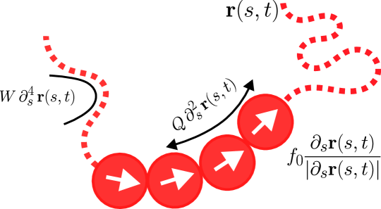
Figure 1: Schematic representation of an active polymer as a succession of active beads. The self-propulsion direction, for each monomer, has constant magnitude and is directed as the backbone tangent vector.

While the system composed by the polymer and the solvent is force-free, as the active colloids are “swimmers”, there is a net force on each monomer composing the backbone of the polymer.
As, according to our construction, the orientations of the beads are constrained, such a force is bound to act along the tangent direction to the backbone. Further, disregarding the depletion of reactants or more complex interactions, the magnitude of the force can be regarded as fixed and independent of the polymer configuration, as it is a characteristic of the monomeric unit. The discretized, bead-spring realisation of such an active polymer model in three dimensions has been investigated numerically in Refs. [46, 53, 54, 55, 56]
We remark that these results are qualitatively different from theoretical calculations[61, 62] and are, for self-avoiding polymers, slightly yet appreciably different from those reported in Refs. [57, 63]. As already suggested in the literature, in cases (ii) and (iii) the magnitude of the active force on each monomer is not strictly homogeneous and it varies within a range. Indeed, the propulsion force is split between neighbours and each monomer (except the ones at the extreme of the polymer) gets a contribution from each bond. The resulting force is proportional to the tangent vector: as such, bent conformations experience a smaller propulsion than straight ones. This difference is probably at the heart of this discrepancy, as will be highlighted by the minimal model tackled in this paper. As such, despite the seemingly formal difference, these qualitative discrepancies may be sufficient to identify case (i) as a different model from (ii) and (iii), at least in three dimensions. From a modeling perspective, one may argue that case (i) could be more suitable if monomers generate their own propulsion or if they are individually pushed by some external agent, such as a molecular motor. Instead, case (ii) and (iii) may be more suitable for coarse-grained representations, where monomers are effective units and the active force may result from the streaming of motors; alternatively, one may consider systems where molecular motors are strong enough to push more than one monomer.

3 Building a continuous minimal active polymer model

In what follows, we will introduce a continuous minimal model for a tangentially active polymer. The polymer is described as a curve $\mathbf{r}(s,t)$, parameterized by the dimensionless contour position $s\in[-N/2,N/2]$ that moves along the polymer backbone, which is subject to active forces, constant in module and related to the polymer conformation. The filament is also subject to random, thermal noise $\boldsymbol{\eta}(s,t)$, that satisfies the usual fluctuation-dissipation relations

$$\left\langle\boldsymbol{\eta}(s,t)\right\rangle=0\qquad\left\langle\boldsymbol{\eta}_{i}(s,t)\boldsymbol{\eta}_{j}(s^{\prime},t^{\prime})\right\rangle=2\mu k_{B}T\delta_{ij}\delta(t-t^{\prime})\delta(s-s^{\prime}).$$ (1)

3.1 Fourier representation

As we will perform most of our analytical calculations in Fourier space, we introduce the standard decomposition in planar waves:

$$\mathbf{r}(s,t)=\frac{1}{\sqrt{N}}\sum_{n=-\infty}^{\infty}\mathbf{r}_{n}(t)e^{\imath k_{n}s}\qquad\boldsymbol{\eta}(s,t)=\frac{1}{\sqrt{N}}\sum_{n=-\infty}^{\infty}\boldsymbol{\eta}_{n}(t)e^{\imath k_{n}s}$$

with $k_{n}=\frac{\pi n}{N}$. We recall that the amplitudes are defined as

$$\mathbf{r}_{n}(t)=\int_{-\frac{N}{2}}^{\frac{N}{2}}\mathbf{r}(s,t)e^{-\imath k_{n}s}ds$$ (2)

and that the chosen basis is not orthonormal

$$\int_{-\frac{N}{2}}^{\frac{N}{2}}e^{\imath(k_{n}-k_{m})s}ds=2\dfrac{\sin(\frac{N}{2}(k_{m}-k_{n}))}{k_{m}-k_{n}}$$ (3)

For $\boldsymbol{\eta}_{n}$ holds

$$\left\langle\boldsymbol{\eta}_{n}(t)\right\rangle=0\qquad\left\langle\boldsymbol{\eta}_{n,i}(t)\boldsymbol{\eta}_{m,j}(t^{\prime})\right\rangle=2\mu k_{B}T\delta_{ij}\delta_{n,m}\delta(t-t^{\prime})$$ (4)

In order to enforce the reality of $\mathbf{r}(s,t)$ and $\eta(s,t)$ we have $\mathbf{r}_{n}=\mathbf{r}_{-n}^{*}$, $\boldsymbol{\eta}_{n}=\boldsymbol{\eta}_{-n}^{*}$.

3.2 Active Rouse Model

In the continuum limit, we model the active polymer by adding the constant tangential force to the usual Rouse model

$$\dot{\mathbf{r}}(s,t)=\mu Q\partial_{s}^{2}\mathbf{r}(s,t)+\mu f_{0}\frac{\partial_{s}\mathbf{r}(s,t)}{|\partial_{s}\mathbf{r}(s,t)|}+\boldsymbol{\eta}(s,t)$$ (5)

$\mu$ is the mobility of the monomers with length $b$, $f_{0}$ is the active force, $Q$ is the strength of the monomer-monomer interactions. We remark that Eq. (5) should be completed with a set of boundary conditions. For the case of free ends, i.e. no forces on the head and tail of the polymer, the boundary conditions read [66, 67]:

$$2Q\partial_{s}\mathbf{r}(s,t)\Big{|}_{s=\pm N/2}=0$$ (6)

In order to get analytical insights of Eq. (5), one typically looks for the eigenfunctions of the operator on the rhs of Eq. (5) that are also compatible with the boundary conditions, Eq. (6). For the case under study, this is a formidable task due to the non-linear forcing term. In order to avoid this difficulty we propose a strong assumption and avoid imposing the boundary conditions summarised in Eq. (6). This amounts to introducing forces and torques on the edges of the polymer whose magnitude, direction and time correlation are, in principle, out of control and can be determined a posteriori.

Accordingly, Eq.(5), in its Fourier representation, reads

$$\sum_{n=-\infty}^{\infty}\dot{\mathbf{r}}_{n}(t)e^{\imath k_{n}s}= -\mu\sum_{n=-\infty}^{\infty}k_{n}^{2}Q\mathbf{r}_{n}(t)e^{\imath k_{n}s}$$

$$+\dfrac{\sum_{n=-\infty}^{\infty}\imath\mu f_{0}k_{n}\mathbf{r}_{n}(t)e^{\imath k_{n}s}}{\sqrt{\sum_{m=-\infty}^{\infty}k_{m}\mathbf{r}_{m}e^{\imath k_{m}s}\cdot\sum_{n=-\infty}^{\infty}k_{n}\mathbf{r}^{*}_{n}e^{-\imath k_{n}s}}}+\sum_{n=-\infty}^{\infty}\boldsymbol{\eta}_{n}(t)e^{\imath k_{n}s}$$ (7)

by multiplying both sides by $e^{-\imath k_{j}s}/N$, using the sum rule (reported in Eq. (38)) and performing the integral in $ds$, we obtain:

$$\sum_{n} \frac{\sin\left(\frac{N}{2}(k_{j}-k_{n})\right)}{N(k_{j}-k_{n})}\dot{\mathbf{r}}_{j}(t)=-\mu\sum_{n}k_{n}^{2}Q\mathbf{r}_{n}(t)\frac{\sin\left(\frac{N}{2}(k_{j}-k_{n})\right)}{N(k_{j}-k_{n})}$$

$$+\frac{\imath\mu f_{0}}{N}\int\dfrac{\sum_{n=-\infty}^{\infty}k_{n}\mathbf{r}_{n}(t)e^{\imath k_{n}s}}{\sqrt{\sum_{m=-\infty}^{\infty}k_{m}\mathbf{r}_{m}e^{\imath k_{m}s}\cdot\sum_{n=-\infty}^{\infty}k_{n}\mathbf{r}^{*}_{n}e^{-\imath k_{n}s}}}e^{-\imath k_{j}s}ds+\boldsymbol{\eta}_{j}(t)$$ (8)

In order to exploit the Fourier analysis we need to explicitly calculate the integral on the rhs of Eq. (3.2). In order to do so we rewrite the denominator as

$$\sum_{m=-\infty}^{\infty}k_{m}\mathbf{r}_{m}e^{\imath k_{m}s}\cdot\sum_{n=-\infty}^{\infty}k_{n}\mathbf{r}_{n}e^{\imath k_{n}s}=\sum_{n=-\infty}^{\infty}k_{n}^{2}\mathbf{r}_{n}\cdot\mathbf{r}_{n}^{*}-\sum_{n=-\infty}^{\infty}\sum_{m\neq-n}k_{m}k_{n}\mathbf{r}_{m}\cdot\mathbf{r}_{n}e^{\imath(k_{m}+k_{n})s}$$ (9)

We remark that at equilibrium, $f_{0}=0$, and we have

$$\langle\mathbf{r}_{n,i}\mathbf{r}_{n,j}\rangle=\delta_{nm}\delta_{ij}\frac{b^{2}N^{2}}{3\pi^{2}}\frac{1}{n^{2}}$$ (10)

Our approach here is to expand the amplitudes around equilibrium. However, by taking Eq. (10) as the zero-order approximation, we observe that the sum on the first term in Eq. (9) is diverging in the limit $n\rightarrow\infty$ whereas the second term remains finite. This implies that the contribution of the active force is always null and the proposed Rouse model cannot capture the coil-to-globule transition observed in the numerical simulations.

3.3 Extended Rouse Model: introducing a finite bending rigidity

In order to overcome this issue, we propose to add a finite bending rigidity

$$\dot{\mathbf{r}}(s,t)=-\mu W\partial_{s}^{4}\mathbf{r}(s,t)+\mu Q\partial_{s}^{2}\mathbf{r}(s,t)+\mu f_{0}\frac{\partial_{s}\mathbf{r}(s,t)}{|\partial_{s}\mathbf{r}(s,t)|}+\boldsymbol{\eta}(s,t)$$ (11)

with boundary conditions [66, 67]

$$\left[2Q\partial_{s}\mathbf{r}(s,t)-W\partial^{3}_{s}\mathbf{r}(s,t)\right]_{s=\pm N/2} =0$$ (12)

$$\left[2\sqrt{\frac{QW}{2}}\partial_{s}\mathbf{r}(s,t)\pm W\partial^{3}_{s}\mathbf{r}(s,t)\right]_{s=\pm N/2} =0$$ (13)

Also in this model, as in the previous one, we avoid imposing the boundary conditions Eq. (13) and, again, this amounts to introducing forces and torques on the edges of the polymer whose magnitude, direction and time correlation are, in principle, out of control and will be determined a posteriori. Notice that the ratio of the bending rigidity, $W$, and the strength of the monomer-monomer interactions $Q$ identifies the persistence length

$$\ell_{p}=b\sqrt{\frac{W}{Q}}$$ (14)

(where $b$ is the monomer length) and the number of Kuhn segments [68]

$$N_{p}=\frac{bN}{\ell_{p}}$$ (15)

In the Fourier representation, Eq. (11) becomes

$$\sum_{n=-\infty}^{\infty}\dot{\mathbf{r}}_{n}(t)e^{\imath k_{n}s}= -\mu\sum_{n=-\infty}^{\infty}k_{n}^{2}\left(Q+Wk_{n}^{2}\right)\mathbf{r}_{n}(t)e^{\imath k_{n}s}$$

$$+\dfrac{\sum_{n=-\infty}^{\infty}\imath\mu f_{0}k_{n}\mathbf{r}_{n}(t)e^{\imath k_{n}s}}{\sqrt{\sum_{m=-\infty}^{\infty}k_{m}\mathbf{r}_{m}e^{\imath k_{m}s}\cdot\sum_{n=-\infty}^{\infty}k_{n}\mathbf{r}^{*}_{n}e^{-\imath k_{n}s}}}+\sum_{n=-\infty}^{\infty}\boldsymbol{\eta}_{n}(t)e^{\imath k_{n}s}$$ (16)

by multiplying both sides by $e^{-\imath k_{j}s}/N$, using the sum rule (reported in Eq. (38)) and integrating in $ds$ we obtain:

$$\sum_{n} \frac{\sin\left(\frac{N}{2}(k_{j}-k_{n})\right)}{N(k_{j}-k_{n})}\dot{\mathbf{r}}_{j}(t)=-\mu\sum_{n}k_{n}^{2}\left(Q+Wk_{n}^{2}\right)\mathbf{r}_{n}(t)\frac{\sin\left(\frac{N}{2}(k_{j}-k_{n})\right)}{N(k_{j}-k_{n})}$$

$$+\frac{\imath\mu f_{0}}{N}\int\dfrac{\sum_{n=-\infty}^{\infty}k_{n}\mathbf{r}_{n}(t)e^{\imath k_{n}s}}{\sqrt{\sum_{m=-\infty}^{\infty}k_{m}\mathbf{r}_{m}e^{\imath k_{m}s}\cdot\sum_{n=-\infty}^{\infty}k_{n}\mathbf{r}^{*}_{n}e^{-\imath k_{n}s}}}e^{-\imath k_{j}s}ds+\boldsymbol{\eta}_{j}(t)$$ (17)

One again we have to deal again with Eq. (9): for this, we now make the following ansatz

$$\underbrace{\sum_{n=-\infty}^{\infty}k_{n}^{2}\mathbf{r}_{n}\cdot\mathbf{r}_{n}^{*}}_{\xi_{0}}\gg-\underbrace{\sum_{n=-\infty}^{\infty}\sum_{m\neq-n}k_{m}k_{n}\mathbf{r}_{m}\cdot\mathbf{r}_{n}e^{\imath(k_{m}+k_{n})s}}_{\xi}$$ (18)

whose validity will also be checked a posteriori. Accordingly, Eq.(3.3) becomes:

$$\sum_{n}\underbrace{\frac{\sin\left(\frac{N}{2}(k_{j}-k_{n})\right)}{N(k_{j}-k_{n})}\dot{\mathbf{r}}_{j}(t)}_{T_{n}}= -\!\!\sum_{n=-\infty}^{\infty}\underbrace{\mu k_{n}^{2}\left(Q+Wk_{n}^{2}\right)\mathbf{r}_{n}(t)\frac{\sin\left(\frac{N}{2}(k_{j}-k_{n})\right)}{N(k_{j}-k_{n})}}_{G_{n}}$$

$$+\!\!\sum_{n=-\infty}^{\infty}\underbrace{2\imath\mu f_{0}\dfrac{k_{n}\mathbf{r}_{n}(t)\frac{\sin\left(\frac{N}{2}(k_{j}-k_{n})\right)}{N(k_{j}-k_{n})}}{\sqrt{\sum_{n=-\infty}^{\infty}k_{n}^{2}\mathbf{r}_{n}(t)\cdot\mathbf{r}_{n}^{*}(t)}}}_{F_{n}}+\boldsymbol{\eta}_{j}(t)$$ (19)

where we have introduced, for convenience, the functions $T_{n}$, $G_{n}$ and $F_{n}$. It is interesting to notice that, at this stage, all terms contribute to the mixing of the modes, not only the non-linear terms $F_{n}$, as one would expect, due to the lack of orthogonality of the chosen basis.

Before proceeding at numerically solving the model, we analyze the functions $T_{n}$, $G_{n}$ and $F_{n}$ in more detail. In order to do so we remark that, at the lowest order, $\langle\mathbf{r}_{n}\mathbf{r}^{*}_{n}\rangle\propto 1/n^{2}$. As such, we focus on modes for which the finite bending rigidity has not become relevant. Indeed, for the higher modes we should assume $\langle\mathbf{r}_{n}\mathbf{r}^{*}_{n}\rangle\propto 1/n^{4}$.[69, 68]
In particular, we look at the relative magnitude of the terms with $n\neq j$ in Eq. (3.3), as compared to the mode $n=j$.

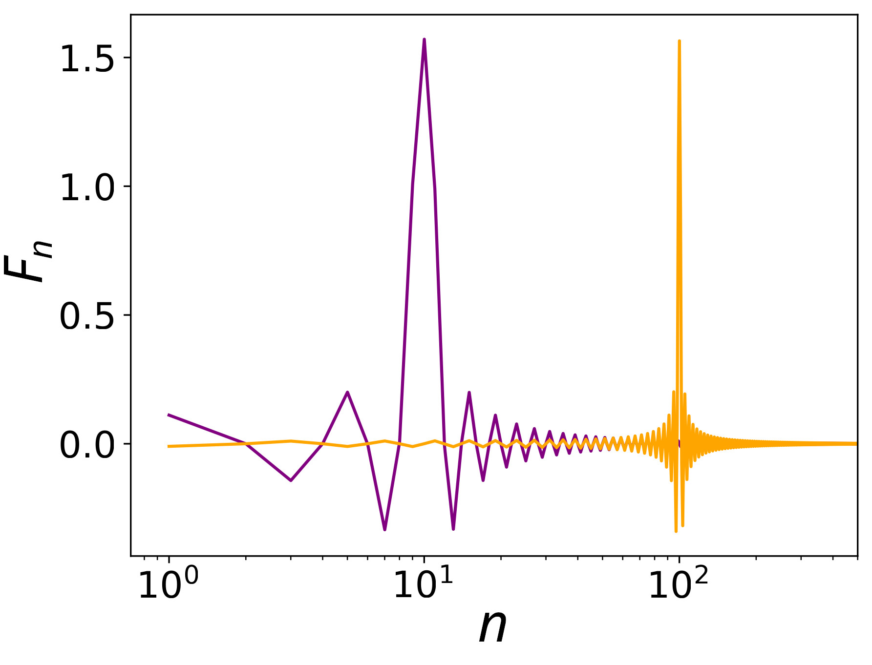
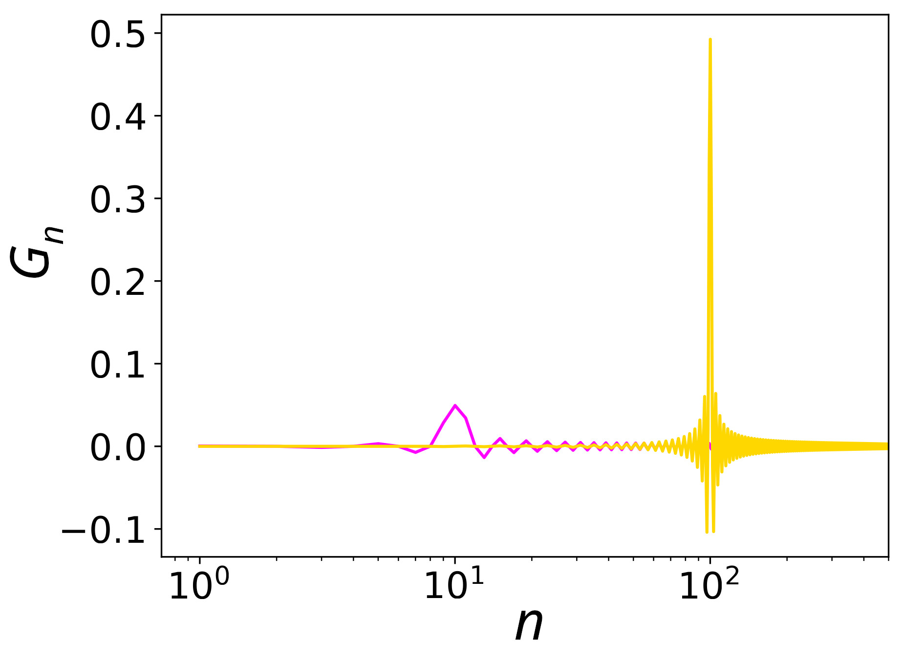
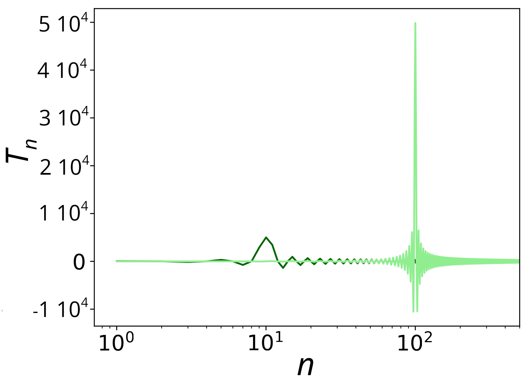
Figure 2: $F_{n}$ (left), $G_{n}$ (center), and $T_{n}$ (right) for $j=10,100$. We remark that $F_{n}$ contributions for $n\simeq 1$ are still relevant even for $j=100$. In contrast, for $T_{n}$ and $G_{n}$ once $j=100$ the modes with $n\simeq 1$ are disregardable.

Figure 2 shows that for $F_{n}$ several modes with $n\neq j$ still provide quite significant contribution to the overall sum as compared to $n=j$. In contrast, for $T_{n}$ and $G_{n}$ the contributions from the modes $n\neq j$ are much smaller and decay quickly, upon moving away from $n=j$. Accordingly, we approximate the sum involving $T_{n}$ and $G_{n}$ with the term with $n=j$ whereas we keep the full sum for $F_{n}$.

Hence we can rewrite Eq. (3.3) as

$$\dot{\mathbf{r}}_{j}(t)=-\mu k_{n}^{2}\left(Q+Wk_{n}^{2}\right)\mathbf{r}_{n}(t)+\sum_{n=-\infty}^{\infty}\frac{2\imath\mu f_{0}k_{n}}{\sqrt{\sum_{n}k_{n}^{2}\mathbf{r}_{n}(t)\cdot\mathbf{r}_{n}^{*}(t)}}\mathbf{r}_{n}(t)\frac{\sin\left(\frac{N}{2}(k_{j}-k_{n})\right)}{N(k_{j}-k_{n})}+\boldsymbol{\eta}_{j}(t)$$ (20)

Eq. (20) represents our minimal model for the active polymer with bending. Finally, recalling that $k_{j}\equiv j\pi/(N)$ where $N$ is the number of monomers, we can rewrite Eq. (20) as

$$\dot{\mathbf{r}}_{j}(t)=-\mu n^{2}(Q_{N}+W_{N}n^{2})+\sum_{n=-\infty}^{\infty}\dfrac{\frac{2}{\pi}\imath\mu f_{0}n}{\sqrt{\sum_{n}n^{2}\mathbf{r}_{n}(t)\cdot\mathbf{r}_{n}^{*}(t)}}\mathbf{r}_{n}(t)\frac{\sin\left(\frac{\pi}{2}(j-n)\right)}{j-n}+\boldsymbol{\eta}_{j}(t)$$ (21)

We note that the last expression is independent of the polymer length $N$, since $N$ only appears in $Q_{N}={Q\pi^{2}}/{N^{2}}$ and $W_{N}={W\pi^{4}}/{N^{4}}$ which, together with $f_{0}$ are the three parameters governing the dynamics of the system. In other words, we can numerically solve (a finite set of) Eqs. (21) for different values of $Q_{N},W_{N}$.Given that

$$\ell_{p}=b\sqrt{\frac{W}{Q}}=\frac{Nb}{\pi}\sqrt{\frac{W_{N}}{Q_{N}}}$$ (22)

and using $\ell_{p}N_{p}=Nb$ leads to

$$N_{p}=\pi\sqrt{\frac{Q_{N}}{W_{N}}}$$ (23)

Accordingly, the ratio $Q_{N}/W_{N}$, is proportional to the number of Kuhn segments.

We numerically integrate these equations using the Euler algorithm, and compute the gyration radius from the steady state value of the correlations among the modes (see Appendix A).

4 Comparison of the gyration ratio predicted in the theory with the gyration ratio from computer simulations

Using the definition of the Kuhn length, the equilibrium expression of the gyration radius for a Gaussian polymer reads [69]:

$$R_{G}=\ell_{p}\sqrt{\frac{N_{p}}{6}}$$ (24)

We aim to compare the predictions of the minimal model Eq. (20) with the results of numerical simulations, reported in the literature[46]. In this context, it is convenient to express the gyration radius (whose dependence on the amplitude of the modes is reported in the Appendix A) in terms of $Q_{N}$ and $W_{N}$

$$R_{G}=\sqrt{\frac{\pi k_{B}T}{2Q_{N}}}\left(\frac{W_{N}}{Q_{N}}\right)^{\frac{1}{4}}$$ (25)

where we used Eqs. (14), (15) and $Q=3k_{B}T/b^{2}$, as in Ref. [69]. Since, as mentioned, Eq. (20) depends only on $f_{0}$, $W_{N}$ and $Q_{N}$, it is tempting to cast the model predictions, as well as the numerical data, in terms of these quantities. Indeed, we find that for the extended Rouse model Eq. (20), the ratio between the gyration radius of an active polymer and its equilibrium value, $R_{G}(N,\text{Pe})/R_{G}(N,0)$, collapse onto a master curve if plotted against the following quantity

$$\text{Pe}_{R}=\frac{f_{0}R_{G}}{k_{B}T}=\frac{f_{0}\ell_{p}}{k_{B}T}\sqrt{\frac{N_{p}}{6}}=\frac{f_{0}b}{k_{B}T}\sqrt{\frac{\pi}{2}\frac{k_{B}T}{b^{2}Q_{N}}}\left(\frac{W_{N}}{Q_{N}}\right)^{\frac{1}{4}}$$ (26)

that is indeed a function of $f_{0}$, $W_{N}$ and $Q_{N}$; $b$ is the monomer size. Eq. (26) shows that polymers with a longer persistence length, characterized by a larger value of $R_{G}$, will be also characterized, at fixed $f_{0}$, by a larger value of $\text{Pe}_{R}$ (see also Appendix D).

Fig.3 reports the model predictions (blue circles) as well as data from simulations of Gaussian (pink downward triangles) and self-avoiding (orange upward triangles) active polymers.

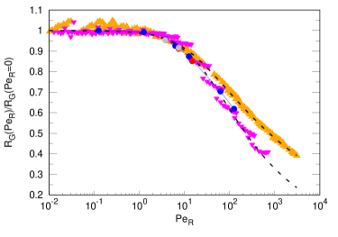
Figure 3: $R_{G}$ normalized by its equilibrium value as a function of $\text{Pe}_{R}$ Eq. (26). Triangles are the data from [46]: orange upward for self-avoiding polymers and pink downwards for Gaussian polymers. Circles are predictions of the Rouse model with bending rigidity Eq. (20) with $Q=0.1$ and $W=0.001$ (blue), $Q=0.1$ and $W=0.002$ (red) and $Q=0.2$ and $W=0.001$ (grey). The dashed lines are a fit to the Gaussian polymer data (pink triangles) with the fitting function Eq. (27) Similarly, upwards black triangles are a fit to the SAW polymer data (orange triangles) with the fitting function Eq. (28).

As shown, plotting $R_{G}(N,\text{Pe})/R_{G}(N,0)$ as a function of $\text{Pe}_{R}$ leads to a collapse of all data. In each curve, we detect a crossover from a plateau to a decay: in the first regime the gyration radius does not depend on the Peclet number, whereas in the second regime the gyration radius decreases with activity, as a signature of a coil-to-globule transition.

Moreover, the data of Rouse model can be well fitted by the following curve (bottom dashed line in Fig.3)

$$R^{Rouse}_{G}(\text{Pe}_{R})=\left(1+\frac{\text{Pe}_{R}}{15}\right)^{-0.21}$$ (27)

whereas the data for the self-avoiding polymer are better fitted by the following curve (top dashed line in Fig.3)

$$R^{SAW}_{G}(\text{Pe}_{R})=\left(1+\frac{\text{Pe}_{R}}{15}\right)^{-0.176}$$ (28)

The scaling functions in Eqs. (27),(28) on the one hand confirm that the Péclet number defined in Eq. (26) is the proper dimensionless number capturing the collapse of the active polymers. On the other hand, they also capture that the value of $\text{Pe}_{R}$ at which the crossover from plateau to collapse occurs is around $\text{Pe}_{R}\simeq 15$ i.e. the “advective” term $f_{0}R_{G}$ should indeed be quite larger then the thermal energy in order to be able to detect the collapse. More in detail the constraint $\text{Pe}_{R}\gg 15$ can be read as

$$\frac{f_{0}b}{k_{B}T}\gg 15\sqrt{\frac{6}{N}}\sqrt{\frac{b}{\ell_{p}}}$$ (29)

which implies that longer $N\gg 1$ and stiffer $\ell_{p}\gg b$ polymers require a weaker value of $f_{0}$ to fulfill the condition in Eq. (29).

Finally, our model has been derived by means of some approximations. In particular the ansatz in Eq. (18) needs to be verified a posteriori. We report such verification in Fig. 4.

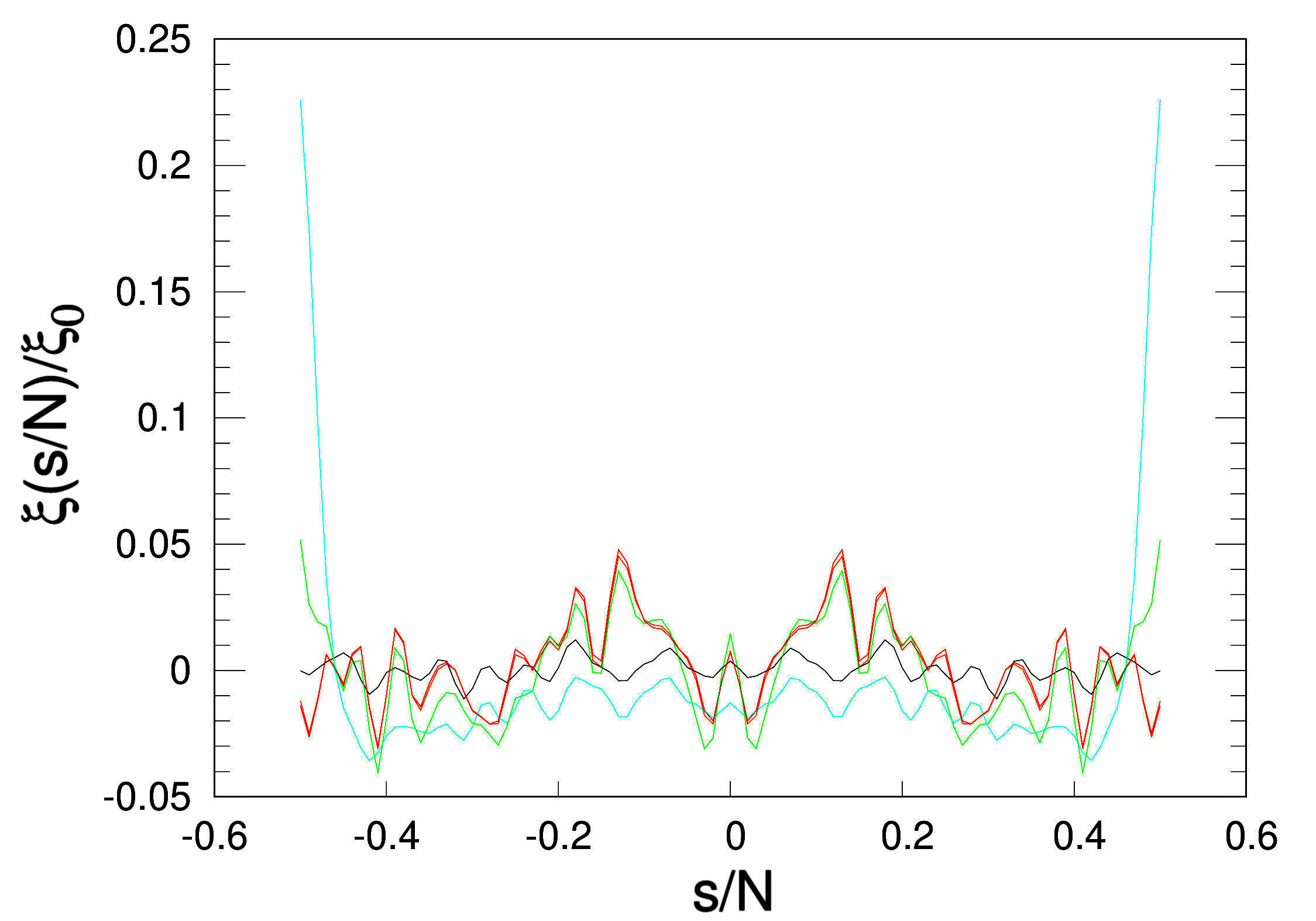
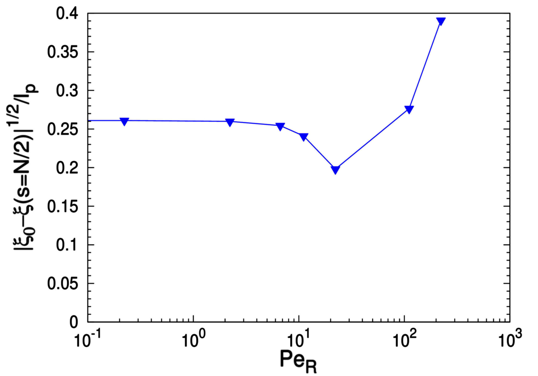
Figure 4: Check of the expansion assumption Eq. (18). Left panel: the value of the force is encoded in color code $f=0,0.1,1,5,10$ for black,red,green,cyan and $\ell_{p}/b=0.1$ Right panel: $\xi/\xi_{0}(s=\pm N/2)$ as a function of the external force.

In the left panel of Fig. 4 we show the test of the assumption as a function of the normalised coordinate along the chain $s/N$ at different values of $f$. Indeed, the ratio $\xi/\xi_{0}$ is small everywhere for $f\lesssim 10$ and, for $f\geq 10$, it increases only in a small region close to the boundaries: overall the condition $\xi\ll\xi_{0}$ remains satisfied. Further, we verify, in the right panel of Fig. 4, that the net force that we apply at the ends is much smaller than the force applied at the middle of the backbone, even at large values of $\text{Pe}_{R}$.

5 Conclusions

In our work we have derived and analyzed an active Rouse model, extended to include finite bending rigidity, that retrieves one of the striking features of the tangentially active polymers with constant propulsion force: namely the collapse of the gyration radius upon increasing the active force on the backbone. The good quantitative agreement between the numerical integration of the active Rouse model and the simulations published in the literature allows us to derive few conclusions. First, our analysis leads us to identify $\text{Pe}_{R}$ as the relevant dimensionless number that allows to collapse all data onto a master curve. Second, once collapsed, the data can be fitted with a simple function that indeed may be employed to make predictions on the collapse of tangentially active polymers. Third, our model identifies the (normalized) tangential force as the term responsible for the correlations among the amplitudes of the Rouse modes. Such non-vanishing correlations indeed lead to the collapse of the gyration radius. Fourth, our model shows that in a pure active Rouse model, without bending rigidity and with an infinite number of modes, the active term would become vanishingly small due to the divergence of the denominator. On the one hand, one could set a cut off for the Rouse modes at some $n$ value. We show that, alternatively, a finite bending rigidity is sufficient in order to keep the active term finite.

However, it is also interesting to notice that the “head-propulsion”, i.e. whether the free ends of the filament are self-propelled or not, has been shown to play a significant role on the steady-state conformations in case (i)[54, 56] where, for coherence, the ends are usually set as passive. On the contrary, in case (ii) and (iii) ends beads are always active. It would be interesting to elucidate the extent of the influence of this aspect, especially towards modelling real biophysical systems. Indeed, as worms and other filamentous organisms live in complex environments[70], it will be of capital importance to develop models able to capture the essential features of their locomotion, for robotic systems[71] as well as for novel generation of filtering devices[72].

Data

The data presented in this contribution can be found here: 10.5281/zenodo.10931600

Appendix A Gyration tensor

The gyration tensor is defined as:

$$S_{ij}(t)=\frac{1}{bN}\int_{-\frac{N}{2}}^{\frac{N}{2}}(\mathbf{r}_{i}(s,t)-\mathbf{r}_{0,i}(t))(\mathbf{r}_{j}(s,t)-\mathbf{r}_{0,j}(t))ds$$ (30)

where $\mathbf{r}_{0}(t)$ is the location of the center of mass. Exploiting the fact that $r$ is a real number, $\mathbf{r}_{m}^{*}=\mathbf{r}_{-m}$, then in the Fourier representation $S$ reads:

$$S_{ij}(t)= \frac{1}{N^{2}}\int_{-\frac{N}{2}}^{\frac{N}{2}}\bigg{[}\sum_{n}\sum_{m}\mathbf{r}_{n,i}(t)\mathbf{r}^{*}_{m,j}(t)e^{\imath k_{n}s}e^{-\imath k_{m}s}-\mathbf{r}_{0,i}(t)\sum_{n}\mathbf{r}^{*}_{n,j}(t)e^{-\imath k_{n}s}$$

$$-\mathbf{r}^{*}_{0,j}(t)\sum_{n}\mathbf{r}_{n,i}(t)e^{\imath k_{n}s}+\mathbf{r}_{0,i}\mathbf{r}^{*}_{0,j}\bigg{]}ds$$ (31)

that, using the sum rule in Eq. (38), reads:

$$S_{ij}(t) =\frac{1}{N^{2}}\int_{-\frac{N}{2}}^{\frac{N}{2}}\sum_{n}\mathbf{r}_{n,i}(t)\mathbf{r}^{*}_{n,j}(t)-\mathbf{r}_{0,i}(t)\mathbf{r}^{*}_{0,j}(t)ds$$

$$=\frac{1}{N}\sum_{n}\mathbf{r}_{n,i}(t)\mathbf{r}^{*}_{n,j}(t)-\mathbf{r}_{0,i}(t)\mathbf{r}^{*}_{0,j}(t)$$

$$=\frac{1}{N}\sum_{n\neq 0}\mathbf{r}_{n,i}(t)\mathbf{r}^{*}_{n,j}(t)$$ (32)

Finally, the gyration radius is defined as $R^{2}_{G}=\text{Tr}S$ and, in equilibrium [69], the amplitudes of the modes is given by Eq. 10. Hence the gyration radius reads

$$R_{G}^{eq}=b\sqrt{\frac{N}{6}}$$ (33)

Appendix B Sum Rule

Coherently with Eq. (3.1) we define

$$\mathbf{r}_{n}(t)=\frac{1}{\sqrt{N}}\int_{-\frac{N}{2}}^{\frac{N}{2}}\mathbf{r}(s,t)e^{-\imath k_{n}s}ds$$ (34)

Substituting Eq. (3.1) into Eq. (34) we get:

$$\mathbf{r}_{n}(t)=\frac{1}{N}\int_{-\frac{N}{2}}^{\frac{N}{2}}\sum_{m=-\infty}^{\infty}\mathbf{r}_{m}(t)e^{\imath k_{m}s}e^{-\imath k_{n}s}ds$$ (35)

and using

$$\int_{-\frac{N}{2}}^{\frac{N}{2}}e^{\imath k_{n}s}e^{-\imath k_{m}s}ds=2\dfrac{\sin(\frac{N}{2}(k_{m}-k_{n}))}{k_{m}-k_{n}}$$ (36)

we get:

$$r_{n}=r_{n}+\frac{2}{N}\sum_{m\neq n}\dfrac{\sin(\frac{N}{2}(k_{m}-k_{n}))}{k_{m}-k_{n}}r_{m}$$ (37)

that leads to:

$$\frac{2}{N}\sum_{m\neq n}\dfrac{\sin(\frac{N}{2}(k_{m}-k_{n}))}{k_{m}-k_{n}}r_{m}=0$$ (38)

Appendix C Convergence of $R_{G}$ upon increasing the number of modes

Fig. 5 shows the convergence of $R_{G}$ upon increasing the number of Rouse modes.

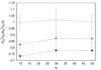
Figure 5: Convergence of $R_{G}$ upon increasing the number of modes (model with bending) for $\beta f_{0}b=0,5,10$ and $\ell_{p}/b=0.1$ standing bigger points for larger values of $f_{0}$.

Appendix D Effective force $\tilde{f}_{0}$

It is interesting to notice that the denominator in the forcing term has the form

$$\sum_{n=-\infty}^{\infty}n^{2}|\mathbf{r}_{n}(t)|^{2}=2\sum_{1}^{\infty}n^{2}|\mathbf{r}_{n}(t)|^{2}$$ (39)

where we accounted for the fact that $|\mathbf{r}_{0}|<\infty$. For a semi-flexible polymer at equilibrium we have

$$|\mathbf{r}_{n}(t)|^{2}\simeq\frac{1}{n^{2}\left(1+\frac{n^{2}}{n^{2}_{p}}\right)}$$ (40)

and hence the sum reads

$$\sum_{n=-\infty}^{\infty}n^{2}|\mathbf{r}_{n}(t)|^{2}=2\sum_{1}^{\infty}\frac{1}{1+\frac{n^{2}}{n^{2}_{p}}}\sim\frac{Nb}{\ell_{p}}$$ (41)

where we used $n_{p}=\frac{Nb}{\ell_{p}}$. This already provides an interesting scaling of the active force with the persistence length. Indeed the relevant parameter is

$$\tilde{f}_{0}\simeq f_{0}\sqrt{\frac{\ell_{p}}{Nb}}$$ (42)

Accordingly, using Eqs. (24),(15), the Péclet number reads:

$$\text{Pe}_{R}=\beta f_{0}R_{G}=\beta\tilde{f}_{0}\frac{bN}{\sqrt{6}}$$ (43)

References

- [1] M.C. Marchetti, J.F. Joanny, S. Ramaswamy, T.B. Liverpool, J. Prost, M. Rao and R.A. Simha, Reviews of modern physics 85 (3), 1143 (2013).
- [2] É. Fodor and M.C. Marchetti, Physica A: Statistical Mechanics and its Applications 504, 106–120 (2018).
- [3] M.E. Cates and J. Tailleur, Annu. Rev. Condens. Matter Phys. 6 (1), 219–244 (2015).
- [4] J. Schwarz-Linek, C. Valeriani, A. Cacciuto, M. Cates, D. Marenduzzo, A. Morozov and W. Poon, Proceedings of the National Academy of Sciences 109 (11), 4052–4057 (2012).
- [5] R. Wittkowski, A. Tiribocchi, J. Stenhammar, R.J. Allen, D. Marenduzzo and M.E. Cates, Nature communications 5 (1), 4351 (2014).
- [6] J. Palacci, S. Sacanna, A. Steinberg, D. Pine and P. Chaikin, Science 339, 936 (2013).
- [7] B. Mognetti, A. Saric, S. Angioletti-Uberti, A. Cacciuto, C. Valeriani and D. Frenkel, Physical Review Letters 111, 245702 (2013).
- [8] L. Cisneros, R. Cortez, C. Dombrowski, R. Goldstein and J. Kessler, Animal Locomotion, Vol. Springer pp. 99–115.
- [9] A. Murugan, J. Zou and M. Brenner, Nat. communications 6, 1 (2015).
- [10] S. Mallory, C. Valeriani and A. Cacciuto, Annual review of physical chemistry 69, 59 (2018).
- [11] V. Narayan, S. Ramaswamy and N. Menon, Science 317, 105 (2007).
- [12] Y. Hayakawa, Europhysics Letters 89, 48004 (2010).
- [13] N. Suematsu, S. Nakata, A. Awazu and H. Nishimori, Physical Review E 81, 056210 (2010).
- [14] D.A. Fletcher and R.D. Mullins, Nature 463 (7280), 485–492 (2010).
- [15] R.D. Vale, Cell 112 (4), 467–480 (2003).
- [16] A. Mahajan, W. Yan, A. Zidovska, D. Saintillan and M.J. Shelley, Physical Review X 12 (4), 041033 (2022).
- [17] A. Goychuk, D. Kannan, A.K. Chakraborty and M. Kardar, Proceedings of the National Academy of Sciences 120 (20), e2221726120 (2023).
- [18] S. Shin, G. Shi, H.W. Cho and D. Thirumalai, Proceedings of the National Academy of Sciences 121 (12), e2307309121 (2024).
- [19] E. Loiseau, S. Gsell, A. Nommick, C. Jomard, D. Gras, P. Chanez, U. D’ortona, L. Kodjabachian, J. Favier and A. Viallat, Nature Physics 16 (11), 1158–1164 (2020).
- [20] B. Chakrabarti, S. Fürthauer and M.J. Shelley, Proceedings of the National Academy of Sciences 119 (4), e2113539119 (2022).
- [21] R. Chelakkot, A. Gopinath, L. Mahadevan and M.F. Hagan, Journal of The Royal Society Interface 11 (92), 20130884 (2014).
- [22] M.K. Faluweki, J. Cammann, M.G. Mazza and L. Goehring, Physical Review Letters 131 (15), 158303 (2023).
- [23] P. Patra, K. Beyer, A. Jaiswal, A. Battista, K. Rohr, F. Frischknecht and U.S. Schwarz, Nature Physics 18 (5), 586–594 (2022).
- [24] J. Rosko, K. Cremin, E. Locatelli, M. Coates, S.J. Duxbury, O.S. Soyer, K. Croft, K. Randall, C. Valeriani and M. Polin, bioRxiv pp. 2024–02 (2024).
- [25] A. Deblais, K. Prathyusha, R. Sinaasappel, H. Tuazon, I. Tiwari, V.P. Patil and M.S. Bhamla, Soft Matter 19 (37), 7057–7069 (2023).
- [26] R. Dreyfus, J. Baudry, M.L. Roper, M. Fermigier, H.A. Stone and J. Bibette, Nature 437 (7060), 862–865 (2005).
- [27] L.J. Hill, N.E. Richey, Y. Sung, P.T. Dirlam, J.J. Griebel, E. Lavoie-Higgins, I.B. Shim, N. Pinna, M.G. Willinger, W. Vogel, J.J. Benkoski, K. Char and J. Pyun, ACS Nano 8 (4), 3272–3284 (2014).
- [28] B. Biswas, R.K. Manna, A. Laskar, S. Kumar P. B., R. Adhikari and G. Kumaraswamy, ACS Nano p. 10025 (2017).
- [29] D. Nishiguchi, J. Iwasawa, H.R. Jiang and M. Sano, New Journal of Physics 20 (1), 015002 (2018).
- [30] M. Kumar, A. Murali, A.G. Subramaniam, R. Singh and S. Thutupalli, arXiv preprint arXiv:2303.10742 (2023).
- [31] A.G. Subramaniam, M. Kumar, S. Thutupalli and R. Singh, arXiv preprint arXiv:2401.14178 (2024).
- [32] Y. Ozkan-Aydin, D.I. Goldman and M.S. Bhamla, Proceedings of the National Academy of Sciences 118 (6), e2010542118 (2021).
- [33] W. Savoie, H. Tuazon, I. Tiwari, M.S. Bhamla and D.I. Goldman, Soft Matter 19 (10), 1952–1965 (2023).
- [34] K. Becker, C. Teeple, N. Charles, Y. Jung, D. Baum, J.C. Weaver, L. Mahadevan and R. Wood, Proceedings of the National Academy of Sciences 119 (42), e2209819119 (2022).
- [35] R.G. Winkler and G. Gompper, The Journal of Chemical Physics 153 (4), 040901 (2020).
- [36] N. Ganai, S. Sengupta and G.I. Menon, Nucleic acids research 42 (7), 4145–4159 (2014).
- [37] J. Smrek and K. Kremer, Physical Review Letters 118 (9), 1–5 (2017).
- [38] J. Smrek, I. Chubak, C.N. Likos and K. Kremer, Nat. Commun. 11 (1), 26 (2020).
- [39] D. Osmanović and Y. Rabin, Soft matter 13 (5), 963–968 (2017).
- [40] A. Kaiser and H. Löwen, The Journal of chemical physics 141 (4) (2014).
- [41] T. Eisenstecken, G. Gompper and R.G. Winkler, Polymers 8 (8), 304 (2016).
- [42] S. Das and A. Cacciuto, Physical Review Letters 123 (8), 087802 (2019).
- [43] L. Theeyancheri, S. Chaki, T. Bhattacharjee and R. Chakrabarti, Physical Review Research 6 (1), L012038 (2024).
- [44] K. Prathyusha, F. Ziebert and R. Golestanian, Soft Matter 18 (15), 2928–2935 (2022).
- [45] R.E. Isele-Holder, J. Elgeti and G. Gompper, Soft Matter 11 (36), 7181–7190 (2015).
- [46] V. Bianco, E. Locatelli and P. Malgaretti, Physical Review Letters 121 (21), 217802 (2018).
- [47] T. Terakawa, S. Bisht, J.M. Eeftens, C. Dekker, C.H. Haering and E.C. Greene, Science 358 (6363), 672–676 (2017).
- [48] G.A. Vliegenthart, A. Ravichandran, M. Ripoll, T. Auth and G. Gompper, Science advances 6 (30), eaaw9975 (2020).
- [49] C. Nguyen, Y. Ozkan-Aydin, H. Tuazon, D.I. Goldman, M.S. Bhamla and O. Peleg, Frontiers in Physics 9, 734499 (2021).
- [50] Z. Mokhtari and A. Zippelius, Physical review letters 123 (2), 028001 (2019).
- [51] S. Das and A. Cacciuto, The Journal of Chemical Physics 151 (24) (2019).
- [52] M. Foglino, E. Locatelli, C. Brackley, D. Michieletto, C. Likos and D. Marenduzzo, Soft matter 15 (29), 5995–6005 (2019).
- [53] E. Locatelli, V. Bianco and P. Malgaretti, Phys. Rev. Lett. 126, 097801 (2021).
- [54] J.X. Li, S. Wu, L.L. Hao, Q.L. Lei and Y.Q. Ma, Physical Review Research 5 (4), 043064 (2023).
- [55] J.P. Miranda, E. Locatelli and C. Valeriani, Journal of Chemical Theory and Computation 20 (4), 1636–1645 (2024).
- [56] M. Vatin, S. Kundu and E. Locatelli, Soft Matter 20 (8), 1892–1904 (2024).
- [57] S.K. Anand and S.P. Singh, Phys. Rev. E 98, 042501 (2018).
- [58] K. Prathyusha, S. Henkes and R. Sknepnek, Physical Review E 97 (2), 022606 (2018).
- [59] L. Abbaspour, A. Malek, S. Karpitschka and S. Klumpp, Physical Review Research 5 (1), 013171 (2023).
- [60] C. Kurzthaler, S. Mandal, T. Bhattacharjee, H. Löwen, S.S. Datta and H.A. Stone, Nature communications 12 (1), 7088 (2021).
- [61] M.S. Peterson, M.F. Hagan and A. Baskaran, Journal of Statistical Mechanics: Theory and Experiment 2020 (1), 013216 (2020).
- [62] C.A. Philipps, G. Gompper and R.G. Winkler, The Journal of Chemical Physics 157 (19) (2022).
- [63] M. Fazelzadeh, E. Irani, Z. Mokhtari and S. Jabbari-Farouji, Phys. Rev. E 108, 024606 (2023).
- [64] M. Fazelzadeh, Q. Di, E. Irani, Z. Mokhtari and S. Jabbari-Farouji, The Journal of Chemical Physics 159 (22), 224903 (2023).
- [65] I. Theurkauff, C. Cottin-Bizonne, J. Palacci, C. Ybert and L. Bocquet, Physical review letters 108 (26), 268303 (2012).
- [66] L. Harnau, R.G. Winkler and P. Reineker, The Journal of Chemical Physics 102 (19), 7750–7757 (1995).
- [67] T. Eisenstecken, G. Gompper and R.G. Winkler, Polymers 8 (2016).
- [68] M. Rubinstein and R.H. Colby, Polymer Physics (Oxfrod university press, Oxford, 2003).
- [69] M. Doi, S.F. Edwards and S.F. Edwards, The theory of polymer dynamics, Vol. 73 (, , 1988).
- [70] A. Kudrolli and B. Ramirez, Proceedings of the National Academy of Sciences 116 (51), 25569–25574 (2019).
- [71] A. Biswas, T. Huynh, B. Desai, M. Moss and A. Kudrolli, Physical Review Fluids 8 (9), 094304 (2023).
- [72] E. Locatelli, V. Bianco, C. Valeriani and P. Malgaretti, Physical Review Letters 131 (4), 048101 (2023).