Axiomatic modeling of fixed proportion technologies

Abstract

Understanding input substitution and output transformation possibilities is critical for efficient resource allocation and firm strategy. There are important examples of fixed proportion technologies where certain inputs are non-substitutable and/or certain outputs are non-transformable. However, there is widespread confusion about the appropriate modeling of fixed proportion technologies in data envelopment analysis. We point out and rectify several misconceptions in the existing literature, and show how fixed proportion technologies can be correctly incorporated into the axiomatic framework. A Monte Carlo study is performed to demonstrate the proposed solution.
Keywords: Data envelopment analysis; Fixed proportion technology; Production theory; Weight restrictions
JEL Codes: C14; C61; D24

1 Introduction

There are several important examples of production technologies where certain inputs are non-substitutable and/or certain outputs are non-transformable. Following [7], in this paper, we refer to such technologies as fixed proportion technologies. In economics, the L-shaped Leontief production function is a classic example of fixed proportion technologies. In manufacturing and services, the use of capital, labor, materials, and energy in fixed proportions is characteristic of production systems [12]. In agricultural production, a primary input (e.g., cocoa beans, wheat seeds) is processed into multiple products in fixed proportions [8].

The axiomatic theory of production that builds upon such works as [13], [11], [14], and [1] is nowadays commonly referred to as data envelopment analysis (DEA) ([9], Charnes1978). DEA does not generally assume anything about substitutability (transformability) among inputs (outputs). However, the empirical DEA frontiers are piece-wise linear surfaces that tend to exhibit at least limited substitution (transformation) possibilities. To improve the DEA estimator in the case of fixed proportion technologies, [7] and [6] propose extended DEA formulations that are claimed to address this issue. Unfortunately, their proposed solution only makes matters worse.

This paper points out and rectifies several errors and misconceptions in the existing literature. We show how fixed proportion technologies can be correctly incorporated into the axiomatic framework. A Monte Carlo study demonstrates the modeling of fixed proportion technologies in DEA falls into the category of finite sample bias and this issue can be addressed by a simple algorithm proposed in this paper.

2 Axiomatic approach

Consider $N$ decision-making units (DMUs). Each DMU operates a joint production technology that transforms $M$ inputs ${\bm{x}}_{n}=(x_{1n},\ldots,x_{Mn})\in\mathbb{R}_{+}^{M}$ to $S$ outputs ${\bm{y}}_{n}=(y_{1n},\ldots,y_{Sn})\in\mathbb{R}_{+}^{S}$, $n=1,\ldots,N$. The most obvious representation of the production technology is the production possibility set ${\mathcal{T}}=\bigl{\{}({\bm{x}},{\bm{y}})\,|\,{\bm{x}}\;{\rm{can}}\,{\rm{produce}}\;{\bm{y}}\bigl{\}}$.

The three classical axioms of the production technology considered in this paper include the following (see, e.g., [13, 1, 10]):

• A1. Free disposability of inputs and outputs: If $({\bm{x}},{\bm{y}})\in{\mathcal{T}}$ and $\tilde{{\bm{x}}}\geq{\bm{x}},\tilde{{\bm{y}}}\leq{\bm{y}}$, then $(\tilde{{\bm{x}}},\tilde{{\bm{y}}})\in{\mathcal{T}}$

• A2. Convexity: If $({\bm{x}},{\bm{y}})\in{\mathcal{T}}$, then $\left(\sum\limits_{n=1}^{N}\lambda_{n}{\bm{x}}_{n},\sum\limits_{n=1}^{N}\lambda_{n}{\bm{y}}_{n}\right)\in{\mathcal{T}}$ for any scalar $\lambda\geq 0$ such that $\sum\limits_{n=1}^{N}\lambda_{n}=1$

• A3. Constant returns to scale: If $({\bm{x}},{\bm{y}})\in{\mathcal{T}}$, then $(\alpha{\bm{x}},\alpha{\bm{y}})\in{\mathcal{T}}$ for any scalar $\alpha>0$

[1] was the first to introduce and prove the minimum extrapolation production functions in the single output case for the following combinations of axioms: A1, {A1, A2}, and {A1, A2, A3}. Extensions to the multiple output setting were presented for A1 in [16] known as the free disposal hull (FDH) technology, for {A1, A2} in [4] known as the variable returns to scale (VRS) or BCC technology, and for {A1, A2, A3} in [9] known as the constant returns to scale (CRS) or CCR technology. The multi-output DEA technologies can be stated in terms of ${\mathcal{T}}$ as follows:

• FDH: $\,{\mathcal{T}}_{\text{A1}}^{\,\text{DEA}}=\Bigl{\{}({\bm{x}},{\bm{y}})\,\Big{|}\,\sum\limits_{n=1}^{N}\lambda_{n}{\bm{x}}_{n}\leq{\bm{x}};\sum\limits_{n=1}^{N}\lambda_{n}{\bm{y}}_{n}\geq{\bm{y}};\sum\limits_{n=1}^{N}\lambda_{n}=1;\lambda_{n}\in\{0,1\},\forall n\Bigl{\}}$

• BCC: $\,{\mathcal{T}}_{\text{A1,A2}}^{\,\text{DEA}}=\Bigl{\{}({\bm{x}},{\bm{y}})\,\Big{|}\,\sum\limits_{n=1}^{N}\lambda_{n}{\bm{x}}_{n}\leq{\bm{x}};\sum\limits_{n=1}^{N}\lambda_{n}{\bm{y}}_{n}\geq{\bm{y}};\sum\limits_{n=1}^{N}\lambda_{n}=1;\lambda_{n}\geq 0,\forall n\Bigl{\}}$

• CCR: $\,{\mathcal{T}}_{\text{A1,A2,A3}}^{\,\text{DEA}}=\Bigl{\{}({\bm{x}},{\bm{y}})\,\Big{|}\,\sum\limits_{n=1}^{N}\lambda_{n}{\bm{x}}_{n}\leq{\bm{x}};\sum\limits_{n=1}^{N}\lambda_{n}{\bm{y}}_{n}\geq{\bm{y}};\lambda_{n}\geq 0,\forall n\Bigl{\}}$

To maintain clarity and brevity, we will focus on the input-oriented CCR technology in the subsequent discussion. Nonetheless, our findings can readily be extended to the BCC and FDH technologies as well as other orientations.

The DEA technology frontier can be estimated by the multiplier form of the CCR model:

$$\max_{{\bm{u}}_{n},{\bm{v}}_{n}}\,\ \theta_{n}=\sum_{s=1}^{S}u_{sn}y_{sn}$$ (1)

$$\mbox{{s.t.}}\quad\sum_{m=1}^{M}v_{mn}x_{mn}=1$$

$$\sum_{s=1}^{S}u_{sn}y_{sj}-\sum_{m=1}^{M}v_{mn}x_{nj}\leq 0,\quad j=1,\ldots,N$$

$$u_{sn}\geq 0,v_{mn}\geq 0,\quad s=1,\ldots,S,\;m=1,\ldots,M$$

where $\theta_{n}$ is a scalar denoting the technical efficiency, ${\bm{v}}_{n}=(v_{1n},\ldots,v_{Mn})\in\mathbb{R}_{+}^{M}$ is a vector of the input weights, and ${\bm{u}}_{n}=(u_{1n},\ldots,u_{Sn})\in\mathbb{R}_{+}^{S}$ is a vector of the output weights for DMU $n$, $n=1,\ldots,N$.

Restrictions on the weights allow for explicitly stating input substitution and output transformation possibilities within the axiomatic approach [2]. In a special case where a pair of inputs are non-substitutable, we may introduce an additional assumption after the maintained axioms:

• A4. Non-substitutability of inputs $m$ and $\tilde{m}$: Either $v_{mn}=0$ or $v_{\tilde{m}n}=0$, $\exists m,\tilde{m}\in\{1,\ldots,M\},\,m\neq\tilde{m},\,\forall n\in\{1,\ldots,N\}$

A4 implies that the ratio of the input weights $v_{mn}/v_{\tilde{m}n}$ must be equal to zero or approach infinity. Analogously, if a pair of outputs are non-transformable, we may introduce another additional assumption:

• A5. Non-transformability of outputs $s$ and $\tilde{s}$: Either $u_{sn}=0$ or $u_{\tilde{s}n}=0$, $\exists s,\tilde{s}\in\{1,\ldots,S\},\,s\neq\tilde{s},\,\forall n\in\{1,\ldots,N\}$

A5 implies that the ratio of the output weights $u_{sn}/u_{\tilde{s}n}$ must be equal to zero or approach infinity. Imposing either A4 or A5 as an additional assumption results in a fixed proportion technology.

It is worth noting that A4 (A5) focuses on the non-substitutability (non-transformability) between a pair of inputs (outputs). It is possible to generalize these axioms to an arbitrary subset of non-substitutable inputs and/or non-transformable outputs, or even multiple subsets of non-substitutable inputs and/or non-transformable outputs. We leave such generalizations as an interesting topic for future research.

3 Correct implementation

If one has prior information and is willing to make additional assumptions that a pair of inputs are non-substitutable (A4) and/or a pair of outputs are non-transformable (A5), we can incorporate those as extra constraints into the CCR multiplier form:

$$\max_{{\bm{u}}_{n},{\bm{v}}_{n}}\,\ \theta_{n}=\sum_{s=1}^{S}u_{sn}y_{sn}$$ (2)

$$\mbox{{s.t.}}\quad\sum_{m=1}^{M}v_{mn}x_{mn}=1$$

$$\sum_{s=1}^{S}u_{sn}y_{sj}-\sum_{m=1}^{M}v_{mn}x_{nj}\leq 0,\quad j=1,\ldots,N$$

$$u_{sn}\geq 0,v_{mn}\geq 0,\quad s=1,\ldots,S,\;m=1,\ldots,M$$

$$\text{either}\;v_{mn}=0\;\text{or}\;v_{\tilde{m}n}=0,\exists m,\tilde{m}\in\{1,\ldots,M\},\,m\neq\tilde{m}$$

$$\text{either}\;u_{sn}=0\;\text{or}\;u_{\tilde{s}n}=0,\exists s,\tilde{s}\in\{1,\ldots,S\},\,s\neq\tilde{s}$$

The formulation of problem (2) is the same as problem (1) except for the final two sets of constraints. The second last set imposes assumption A4, enforcing the marginal rate of substitution (MRS) between the pair of non-substitutable inputs to be either zero or infinite. The last set of constraints imposes A5, enforcing the marginal rate of transformation (MRT) between the pair of non-transformable outputs to be either zero or infinite.

Problem (2) is a disjunctive programming problem, which is computationally demanding due to the need for specialized optimization solvers. Fortunately, there exists a simple branch-and-cut algorithm that breaks down problem (2) into a stepwise procedure. This method, which we will refer to as FP-constrained DEA, offers a more accessible approach. Without the loss of generality, consider a basic scenario with two inputs and a single output, where the two inputs are non-substitutable. Based on this scenario, the stepwise procedure of FP-constrained DEA is demonstrated in Algorithm 1.

Data: $\{{\bm{x}}_{n},y_{n}\}_{n=1}^{N}\in\mathbb{R}_{+}^{2}\times\mathbb{R}_{+}$

1 $\theta_{n}=0,n=1,\ldots,N$;

2 while $\theta_{n}=0$ do

3       Solve problem (1) excluding $x_{1n}$ while keeping all other variables to calculate $\theta_{n}^{1}$;

4      Solve problem (1) excluding $x_{2n}$ while keeping all other variables to calculate $\theta_{n}^{2}$; if $\theta_{n}^{1}\geq\theta_{n}^{2}$ then

5             $\theta_{n}=\theta_{n}^{1}$;

6            

7      else

8             $\theta_{n}=\theta_{n}^{2}$;

9            

10      

Result: $\theta_{n}$

Algorithm 1 Calculating technical efficiency $\theta_{n}$ using FP-constrained DEA.

4 Monte Carlo simulations

Consider a fixed proportion technology with $M$ inputs and a single output, where the true production function is $F({\bm{x}}_{n})=\min\{x_{1n},\ldots,x_{Mn}\},n=1,\ldots,N$. The inputs are randomly generated from the uniform distribution in the range $[0,100]$. The observed output $y_{n}=F({\bm{x}}_{n})\times\exp(-\mu_{n})$ is perturbed by a half-normal inefficiency term $\mu_{n}\geq 0$ drawn independently from $\mathcal{N}^{+}(0,\sigma_{\mu}^{2})$. No stochastic noise is considered as standard DEA does not handle it. The fixed proportion technology is assumed to exhibit CRS, and the technology frontier is characterized by the Shephard input distance function. Once the frontier is estimated, it is possible to measure efficiency using various types of distance metrics or slack-based measures, but this is another question that is not dependent on frontier estimation. In this study, we do not consider non-radial slacks but simply use the radial Farrell measure of technical efficiency.

We examine 48 scenarios encompassing input dimensions $M\in\{2,3\}$, no inefficiency and 3 levels of inefficiency with standard deviations $\sigma_{\mu}\in\{1,2,3\}$, along with 6 different sample sizes $N\in\{30,50,100,300,500,1000\}$. Each scenario is replicated 1000 times using the DEA toolbox developed by [3] on MATLAB R2021a. The computation was undertaken on the Viking Cluster, a high performance computing facility provided by the University of York.

Since we know the true distance to the frontier of the fixed proportion technology, we can compare the finite sample performance of the original CCR DEA and our proposed FP-constrained DEA relative to the true frontier. In addition, we include [7]’s (Barnum2011) proposed modeling of fixed proportion technologies in this comparison. [7] and [6] impose identical input (output) weights between any pair of non-substitutable inputs (non-transformable outputs) in the CCR and BBC DEA formulations, respectively. Technically, perfect substitutability (transformability) between inputs (outputs) is a direct consequence of this modeling approach. In other words, their results would be exactly the same if perfect substitutability (transformability) was assumed.

A standard performance measure is the mean squared error (MSE) between the true and estimated distance to the frontier (technical efficiency scores). The smaller the MSE, the better the finite sample performance. Table 1 presents the MSE statistics for different methods across diverse scenarios.

Table 1: MSE statistics for CCR DEA (CCR), FP-constrained DEA (FP), and [7]’s (Barnum2011) proposal (BG).

$M$ $N$ $\sigma_{\mu}=1$ $\sigma_{\mu}=2$ $\sigma_{\mu}=3$ no inefficiency CCR FP BG CCR FP BG CCR FP BG CCR & FP BG 2 30 0.0076 0.0035 0.0619 0.0120 0.0068 0.0344 0.0146 0.0093 0.0248 0 0.2230 50 0.0038 0.0014 0.0631 0.0061 0.0028 0.0340 0.0076 0.0041 0.0234 0 0.2231 100 0.0013 0.0004 0.0668 0.0021 0.0008 0.0358 0.0026 0.0011 0.0239 0 0.2251 300 0.0003 0.0000 0.0701 0.0004 0.0001 0.0382 0.0006 0.0002 0.0256 0 0.2265 500 0.0001 0.0000 0.0717 0.0002 0.0000 0.0392 0.0002 0.0001 0.0263 0 0.2268 1000 0.0000 0.0000 0.0732 0.0001 0.0000 0.0403 0.0001 0.0000 0.0273 0 0.2270 3 30 0.0189 0.0071 0.0890 0.0261 0.0136 0.0485 0.0291 0.0177 0.0340 0 0.3311 50 0.0097 0.0029 0.0916 0.0134 0.0056 0.0485 0.0153 0.0076 0.0325 0 0.3360 100 0.0042 0.0008 0.0985 0.0058 0.0017 0.0525 0.0068 0.0024 0.0349 0 0.3439 300 0.0010 0.0001 0.1056 0.0014 0.0002 0.0569 0.0017 0.0003 0.0379 0 0.3519 500 0.0005 0.0000 0.1081 0.0007 0.0001 0.0586 0.0009 0.0001 0.0392 0 0.3549 1000 0.0002 0.0000 0.1109 0.0003 0.0000 0.0607 0.0004 0.0000 0.0409 0 0.3568

In the case of no inefficiency, both CCR DEA and FP-constrained DEA achieve a perfect fit for all input dimensions and sample sizes, whereas [7]’s (Barnum2011) proposal yields estimates noticeably deviating from the true technical efficiency scores. In the presence of inefficiencies, CCR DEA demonstrates strong performance in estimating fixed proportion technologies, as evidenced by low MSE values. Impressively, FP-constrained DEA outperforms even further, achieving MSE values that are closer to zero. In sharp contrast, [7]’s (Barnum2011) proposal exhibits notably diminished performance. These findings are further confirmed by the correlation coefficients between the true distance to the frontier and the estimates, as reported in Table 2. More detailed findings in the presence of inefficiencies are summarized as follows:

• The finite sample performance of both CCR DEA and FP-constrained DEA becomes slightly worse as the standard deviation of inefficiency increases or an additional input is included.

• As the sample size increases, both CCR DEA and FP-constrained DEA exhibit reduced MSE values and increased correlation coefficients, thus signifying enhanced finite sample performance.

• FP-constrained DEA, in comparison to CCR DEA, achieves consistently better finite sample performance, particularly in small samples.

Overall, the Monte Carlo study has provided numerical evidence 1) that the original CCR DEA modeling of fixed proportion technologies suffers from finite sample bias but approaches the true frontier as the sample size increases and 2) that our proposed FP-constrained DEA approach offers more accurate modeling of fixed proportion technologies and alleviates finite sample bias, particularly in small samples.

Table 2: Correlation coefficients for CCR DEA (CCR), FP-constrained DEA (FP), and [7]’s (Barnum2011) proposal (BG).

$m$ $N$ $\sigma_{u}=1$ $\sigma_{u}=2$ $\sigma_{u}=3$ CCR FP BG CCR FP BG CCR FP BG 2 30 0.9862 0.9941 0.6836 0.9859 0.9920 0.8092 0.9839 0.9896 0.8501 50 0.9917 0.9976 0.6865 0.9914 0.9964 0.8121 0.9901 0.9949 0.8521 100 0.9967 0.9993 0.6887 0.9965 0.9989 0.8131 0.9958 0.9984 0.8524 300 0.9990 0.9999 0.6878 0.9989 0.9998 0.8123 0.9987 0.9997 0.8514 500 0.9995 1.0000 0.6883 0.9994 0.9999 0.8126 0.9993 0.9999 0.8516 1000 0.9998 1.0000 0.6875 0.9998 1.0000 0.8120 0.9997 1.0000 0.8511 3 30 0.9608 0.9844 0.5944 0.9645 0.9795 0.7422 0.9628 0.9750 0.7949 50 0.9770 0.9935 0.6057 0.9797 0.9910 0.7479 0.9782 0.9882 0.7977 100 0.9882 0.9979 0.6009 0.9892 0.9968 0.7421 0.9882 0.9955 0.7909 300 0.9961 0.9997 0.6027 0.9963 0.9995 0.7433 0.9959 0.9993 0.7916 500 0.9977 0.9999 0.6023 0.9978 0.9998 0.7429 0.9975 0.9997 0.7912 1000 0.9989 1.0000 0.6030 0.9989 1.0000 0.7433 0.9988 0.9999 0.7914

Note: Correlation coefficients in the case of no inefficiency are undefined as the true technical efficiency scores consistently equal 1.

To gain more insight, we proceed to plot the true input isoquants and those estimated by CCR DEA and FP-constrained DEA, as well as [7]’s (Barnum2011) proposal, based on random samples of the two extreme sample sizes in this study (30 and 1000) within the scenarios of two inputs. Figures 1 and 2 illustrate the four sets of input isoquants with the smallest (30) and largest (1000) sample sizes, respectively.

Both figures highlight the misconceptions of [7]’s (Barnum2011) proposal. It benchmarks the data points relative to the green line with the slope of $-1$ in all scenarios. This observation is entirely in line with our expectations, as we have established this conclusion above that [7]’s (Barnum2011) proposal would lead to exactly the same result if perfect substitutability was assumed. Clearly, it does not capture the correct shape of the input isoquant, even if we have perfectly accurate data with zero noise and inefficiency (as shown in panels 1(a) and 2(a)). In contrast, both CCR DEA and FP-constrained DEA achieve a perfect fit to the true input isoquant in the case of no inefficiency.

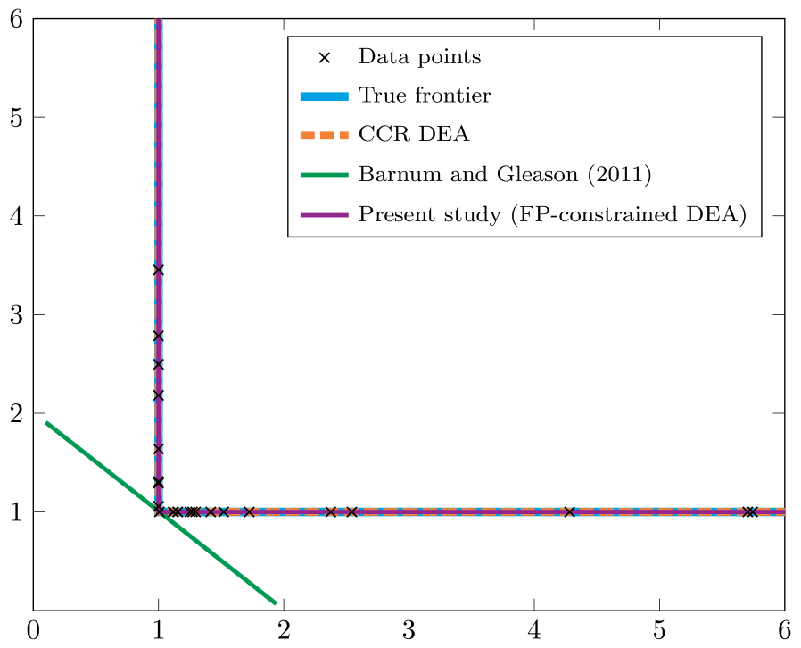
(a) no inefficiency

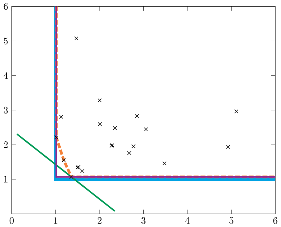
(b) $\sigma_{\mu}=1$

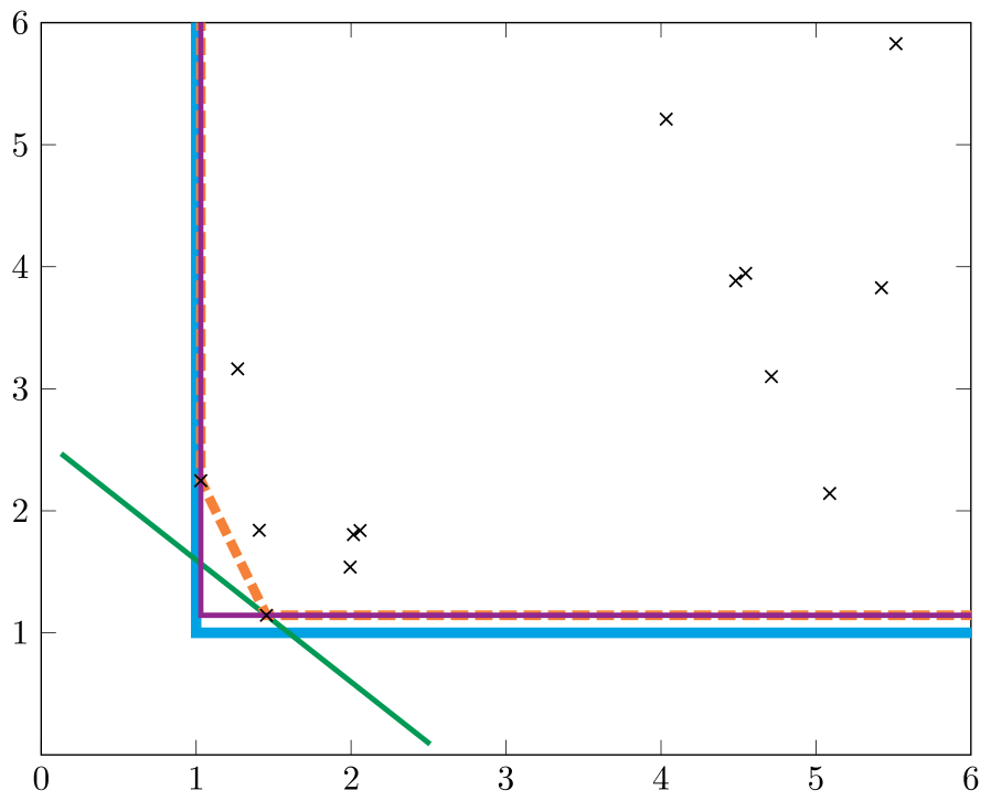
(c) $\sigma_{\mu}=2$

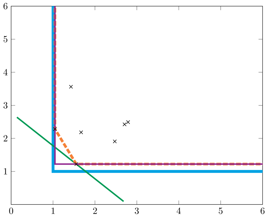
(d) $\sigma_{\mu}=3$

Figure 1: Illustration of the input isoquants estimated by CCR DEA, FP-constrained DEA, and [7]’s (Barnum2011) proposal with $N=30$.

Combining Figures 1 and 2, when inefficiencies are present, one can correctly argue that CCR DEA produces a wrong shape of the input isoquant with a small sample size (e.g., 30), yet the CCR DEA frontier converges to the true frontier when the sample size is sufficiently large (e.g., 1000). In contrast, FP-constrained DEA can mimic the correct shape of the true frontier even in a small sample and further, it performs consistently better than CCR DEA.

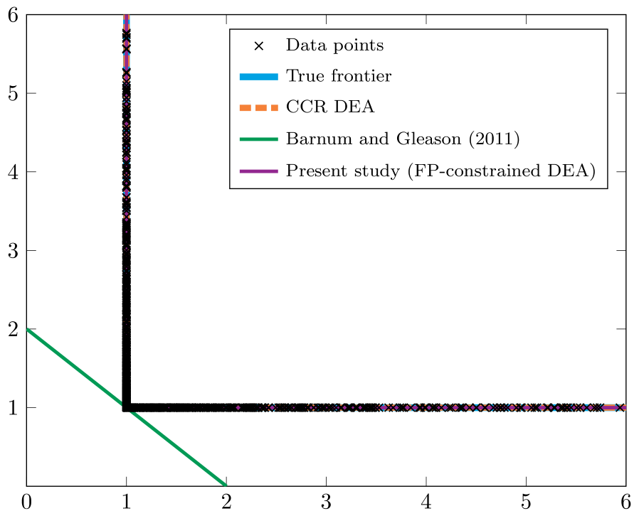
(a) no inefficiency

(b) $\sigma_{\mu}=1$

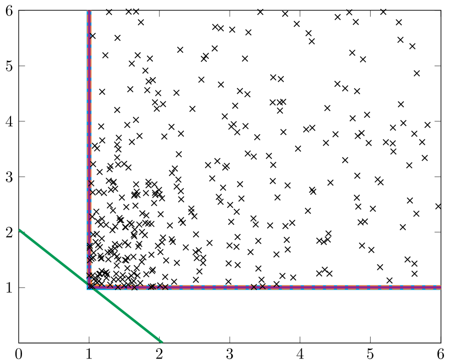
(c) $\sigma_{\mu}=2$

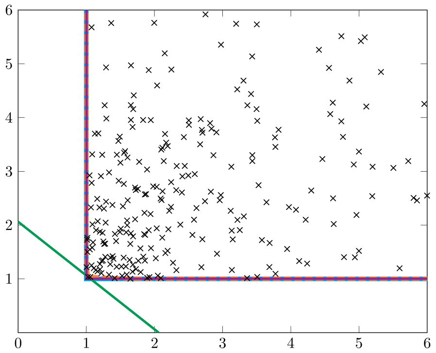
(d) $\sigma_{\mu}=3$

Figure 2: Illustration of the input isoquants estimated by CCR DEA, FP-constrained DEA, and [7]’s (Barnum2011) proposal with $N=1000$.

5 Conclusions

[7] and [6] argue that DEA is inappropriate for estimating fixed proportion technologies because DEA implicitly assumes inputs are substitutable and outputs are transformable. In fact, nothing in the classical axioms of DEA limits substitutability or transformability. We agree with the conceptual point that if the true frontier of the underlying technology is L-shaped, the DEA frontier might have a wrong shape. That being said, this issue is merely finite sample bias. Going back to the classic works in economics by [13] and [1] and the DEA literature later developed by [5] and [15], we know that DEA is statistically consistent under axioms A1–A3. Since the fixed proportion technology does satisfy all the axioms, DEA is consistent in this case.

In this paper, we have proposed the correct modeling of fixed proportion technologies within the axiomatic framework. A Monte Carlo study confirms the finite sample bias in the DEA modeling of fixed proportion technologies and the superiority of our proposed FP-constrained DEA over the original CCR DEA. If one does not have prior information about the substitution or transformation possibilities but the assumptions of DEA hold, then it is better to use standard DEA because it is consistent for the entire range between perfect substitution (transformation) as one extreme case and non-substitution (non-transformation) as the other extreme. The finite sample bias can be alleviated by simply increasing the sample size. However, if one needs to make an additional assumption on the substitution or transformation possibilities, FP-constrained DEA can more accurately model fixed proportion technologies not only in large samples but notably in small ones.

We believe that this paper opens interesting avenues for future research. The proposed FP-constrained DEA can readily be extended to various DEA models. It is possible to generalize the fixed proportion axioms to one or more arbitrary subsets of non-substitutable inputs and/or non-transformable outputs. Such subsets might also include undesirable outputs and thus, it would be relevant to consider alternative axioms such as weak disposability. Extension to convex regression and related techniques is also left as an interesting challenge for future research.

References

- [1] S.. Afriat “Efficiency Estimation of Production Functions” In International Economic Review 13.3, 1972, pp. 568–598
- [2] R. Allen, A. Athanassopoulos, R.. Dyson and E. Thanassoulis “Weights restrictions and value judgements in Data Envelopment Analysis: Evolution, development and future directions” In Annals of Operations Research 73, 1997, pp. 13–34
- [3] Inmaculada C. Álvarez, Javier Barbero and José L. Zofío “A Data Envelopment Analysis Toolbox for MATLAB” In Journal of Statistical Software 95.3, 2020
- [4] R.. Banker, A. Charnes and W.. Cooper “Some Models for Estimating Technical and Scale Inefficiencies in Data Envelopment Analysis” In Management Science 30.9, 1984, pp. 1078–1092
- [5] Rajiv D. Banker “Maximum Likelihood, Consistency and Data Envelopment Analysis: A Statistical Foundation” In Management Science 39.10, 1993, pp. 1265–1273
- [6] Darold Barnum et al. “Impact of input substitution and output transformation on data envelopment analysis decisions” In Applied Economics 49.15, 2017, pp. 1543–1556
- [7] Darold Barnum and John Gleason “Measuring efficiency under fixed proportion technologies” In Journal of Productivity Analysis 35.3, 2011, pp. 243–262
- [8] Onur Boyabatlı “Supply Management in Multiproduct Firms with Fixed Proportions Technology” In Management Science 61.12, 2015, pp. 3013–3031
- [9] A. Charnes, W.. Cooper and E. Rhodes “Measuring the efficiency of decision making units” In European Journal of Operational Research 2.6, 1978, pp. 429–444
- [10] Rolf Färe and Daniel Primont “Multi-Output Production and Duality: Theory and Applications” Boston: Kluwer Academic Publishers, 1995
- [11] M.. Farrell “The measurement of productive efficiency” In Journal of the Royal Statistical Society. Series A (General) 120.3, 1957, pp. 253–290
- [12] Samet Güner and Halil İbrahim Cebeci “Multi-period efficiency analysis of major European and Asian airports under fixed proportion technologies” In Transport Policy 107, 2021, pp. 24–42
- [13] Tjalling Charles Koopmans “An analysis of production as an efficient combination of activities” In Activity Analysis of Production and Allocation New York: Wiley, 1951
- [14] Ronald W Shephard “Theory of Cost and Production Functions” Princeton, New Jersey: Princeton University Press, 1970
- [15] Léopold Simar “Aspects of statistical analysis in DEA-type frontier models” In Journal of Productivity Analysis 7.2-3, 1996, pp. 177–185
- [16] Henry Tulkens “On FDH Efficiency Analysis: Some Methodological Issues and Applications to Retail Banking, Courts, and Urban Transit” In Journal of Productivity Analysis 4, 1993, pp. 183–210