Matching the Statistical Query Lower Bound for k-sparse Parity Problems with Stochastic Gradient Descent

Abstract

The $k$-parity problem is a classical problem in computational complexity and algorithmic theory, serving as a key benchmark for understanding computational classes. In this paper, we solve the $k$-parity problem with stochastic gradient descent (SGD) on two-layer fully-connected neural networks. We demonstrate that SGD can efficiently solve the $k$-sparse parity problem on a $d$-dimensional hypercube ($k\leq O(\sqrt{d})$) with a sample complexity of $\widetilde{O}(d^{k-1})$ using $2^{\Theta(k)}$ neurons, thus matching the established $\Omega(d^{k})$ lower bounds of Statistical Query (SQ) models. Our theoretical analysis begins by constructing a good neural network capable of correctly solving the $k$-parity problem. We then demonstrate how a trained neural network with SGD can effectively approximate this good network, solving the $k$-parity problem with small statistical errors. Our theoretical results and findings are supported by empirical evidence, showcasing the efficiency and efficacy of our approach.

1 Introduction

The $k$-parity problem, defined on a binary sequence of length $d$, is fundamental in the field of computational complexity and algorithmic theory. This problem involves the analysis of parity conditions in a subset of cardinality $k$ by assessing if the occurrence of $1$’s in this subset is even or odd. The complexity of the problem escalates as the parameter $k$ increases. Its significance, while evidently practical, is rooted in its theoretical implications; it serves as a vital benchmark in the study of computational complexity classes and has profound implications for our understanding of P versus NP (Vardy, 1997; Downey et al., 1999; Dumer et al., 2003) and other cornerstone questions in computational theory (Blum, 2005; Klivans et al., 2006). Furthermore, the $k$-parity problem’s complexity underpins significant theoretical constructs in error detection and information theory (Dutta et al., 2008), and is instrumental in delineating the limitations and potential of algorithmic efficiency (Farhi et al., 1998). This paper tackles the $k$-sparse parity problem (Daniely and Malach, 2020), where the focus is on the parity of a subset with cardinality $k\ll d$.

Recent progress in computational learning theory has focused on improving the sample complexity guarantees for learning $k$-sparse parity functions using stochastic gradient descent (SGD). Under the framework of the Statistical Query (SQ) model (Kearns, 1998), it has been established that learning the $k$-sparse parity function requires a minimum of $\Omega(d^{k})$ queries (Barak et al., 2022), highlighting the challenge in efficiently learning these functions. In particular, for a neuron network trained by SGD algorithm, the total number of scalar queries required is $m\cdot d\cdot n$, where $m$ is the number of neurons, $d$ is the dimension, $m\cdot d$ is the total number of scalar queries used for one example, and $n$ is the total number of fresh examples required in the algorithm. Considerable effort has been devoted to establishing sample complexity upper bounds for the special XOR case ($k=2$), with notable successes including $O(d)$ sample complexity using infinite-width or exponential-width ($O(2^{d})$) two-layer neural networks trained via gradient flow (Wei et al., 2019; Chizat and Bach, 2020; Telgarsky, 2022), and $O(d^{2})$ sample complexity with polynomial-width networks via SGD (Ji and Telgarsky, 2020; Telgarsky, 2022). A significant advancement in solving the $2$-parity problem was recently introduced by Glasgow (2023). They proved a sample complexity bound of $\widetilde{O}(d)$ using a two-layer ReLU network with logarithmic width trained with SGD, thus matching the SQ lower bound.

In the general case of $k\geq 2$, Barak et al. (2022) has marked significant progress, achieving a sample complexity of $\widetilde{O}(d^{k+1})$ with a network width requirement of $2^{\Theta(k)}$, which is independent of the input dimension $d$. Additionally, Barak et al. (2022) demonstrated that the neural tangent kernel (NTK)-based method (Jacot et al., 2018) requires a network of polynomial width $d^{\Omega(k)}$ to solve the $k$-parity problem. In a recent work, Suzuki et al. (2023) attained a sample complexity of $O(d)$. However, it is important to note that they employed the mean-field Langevin dynamics (MFLD) (Mei et al., 2018; Hu et al., 2019), which requires neural networks of exponential width $O(e^{d})$, and an $O(e^{d})$ number of iterations to converge. Thus, their method is not computationally practical and doesn’t match the statistical query lower bound. Abbe et al. (2023a) introduced the leap-$k$ function for binary and Gaussian sequences, which extended the scope of the $k$-parity problem. They also proved Correlational Statistical Query (CSQ) lower bounds for learning leap-$k$ function with both Gaussian and Boolean input. They proved novel CSQ lower bounds of $\Omega(d^{k-1})$ for Boolean input in Proposition 30 and $\Omega(d^{k/2})$ for Gaussian input in Proposition 31, which suggests that learning from Boolean input can be intrinsically harder than learning from Gaussian input. They also proved SGD can learn low dimensional target functions with Gaussian isotropic data and 2-layer neural networks using $n\gtrsim d^{\mathrm{Leap}-1}$ examples. However, their upper bound analysis is based on the assumption that the input data $\mathbf{x}$ follows a Gaussian distribution and relies on Hermite polynomials, making it unclear how to extend them to analyze Boolean input. This raises a natural but unresolved question:

Is it possible to match the statistical query lower bound for $k$-sparse parity problems with stochastic gradient descent?

In this paper, we give an affirmative answer to the above question. In particular, we consider the standard $k$-sparse parity problem, where the input $\mathbf{x}$ is drawn from a uniform distribution over $d$-dimensional hypercube $\mathrm{Unif}(\{-1,1\}^{d})$. Our approach involves training two-layer fully-connected neural networks with $m=2^{\Theta(k)}$ width using SGD with a batch size of $B=O(d^{k-1}\operatorname{\rm polylog}(d))$. We prove that the neural network can achieve a constant-order positive margin with high probability after training for $T=O(\log d)$ iterations. Therefore, the total number of examples required in our approach is $n=BT=\widetilde{O}(d^{k-1})$. The total number of scalar queries required in our paper is $m\cdot d\cdot n=2^{\Theta(k)}\cdot d\cdot(d^{k-1}\cdot\text{polylog}d)=2^{\Theta(k)}d^{k}\cdot\text{polylog}d$, where $m$ is the number of neurons, $d$ is the dimension, $m\cdot d$ is the total number of scalar queries used for one example, and $n$ is the total number of fresh examples required in our algorithm. Abbe et al. (2023a) also gave a CSQ lower bound in Proposition 30 for learning $d$-dimensional uniform Boolean data, which leads to the sample complexity lower bound $n\gtrsim d^{k-1}$. Thus, we also match the CSQ lower bound in Abbe et al. (2023a).

1.1 Our Contributions

The Statistical Query (SQ) lower bound demonstrates that, regardless of architecture, gradient descent requires a query complexity of $\Omega(d^{k})$ for learning $k$-sparse $d$-dimensional parities under a constant noise level. We push the sample complexity frontier of $k$-sparse party problem to $\widetilde{O}(d^{k-1})$ via SGD, specifically with online stochastic sign gradient descent. Notably, for the XOR problem ($k=2$) which is a special case of $k$-parities, Glasgow (2023) achieved a sample complexity of $\widetilde{O}(d)$ via SGD. Nevertheless, the algorithm and analysis used in our paper is quite different from theirs. Our main result is stated in the following informal theorem:

Theorem 1.1 (Informal)

Utilizing sign SGD with a batch size of $\widetilde{O}(d^{k-1})$ on two-layer fully-connected neural networks of width $2^{\Theta(k)}$, we can find a solution to the $k$-parity problem with a small test error in $O(k\log d)$ iterations.

The above theorem improves the sample complexity in Barak et al. (2022) from $\widetilde{O}(d^{k+1})$ to $\widetilde{O}(d^{k-1})$. Moreover, the total number of queries required is $\widetilde{O}(d^{k})$ which matches the SQ/CSQ lower bound up to logarithmic factors. Additionally, this result matches the best sample complexity when solving $2$-parity problem (Glasgow, 2023). It is worth noting that our results only require two-layer fully connected neural networks with $2^{\Theta(k)}$ width and SGD training with $O(k\log d)$ iterations, which gives an efficient algorithm.

Notation.

We use $[N]$ to denote the index set $\{1,\dots,N\}$. We use lowercase letters, lowercase boldface letters, and uppercase boldface letters to denote scalars, vectors, and matrices, respectively. For a vector $\mathbf{v}=(v_{1},\cdots,v_{d})^{\top}$, we denote by $\|\mathbf{v}\|_{2}:=(\sum_{j=1}^{d}v_{j}^{2})^{1/2}$ its $L_{2}$ norm. For a vector $\mathbf{v}=(v_{1},\cdots,v_{d})^{\top}$, we denote by $\mathbf{v}_{[i_{1}:i_{2}]}:=(v_{i_{1}},\cdots,v_{i_{2}})^{\top}$ its truncated vector ranging from the $i_{1}$-th coordinate to the $i_{2}$-th coordinate. For two sequence $\{a_{k}\}$ and $\{b_{k}\}$, we denote $a_{k}=O(b_{k})$ if $|a_{k}|\leq C|b_{k}|$ for some absolute constant $C$, denote $a_{k}=\Omega(b_{k})$ if $b_{k}=O(a_{k})$, and denote $a_{k}=\Theta(b_{k})$ if $a_{k}=O(b_{k})$ and $a_{k}=\Omega(b_{k})$. We also denote $a_{k}=o(b_{k})$ if $\lim|a_{k}/b_{k}|=0$. We use $\widetilde{O}(\cdot)$ and $\widetilde{\Omega}(\cdot)$ to omit logarithmic terms in the notation. Finally, we denote $x_{n}=\mathrm{poly}(y_{n})$ if $x_{n}=\mathcal{O}(y_{n}^{D})$ for some positive constant $D$, and $x_{n}=\operatorname{\rm polylog}(y_{n})$ if $x_{n}=\mathrm{poly}(\log(y_{n}))$.

2 Related Work

XOR.

The performance of two-layer neural networks in the task of learning $2$-parity has been the subject of extensive research in recent years. Wei et al. (2019); Chizat and Bach (2020); Telgarsky (2022) employed margin techniques to establish the convergence toward a global margin maximization solution, utilizing gradient flow and sample complexity of $O(d)$. Notably, Wei et al. (2019) and Chizat and Bach (2020) employed infinite-width neural networks, while Telgarsky (2022) employed a more relaxed width condition of $O(d^{d})$. A significant breakthrough in this domain was achieved by Glasgow (2023), who demonstrated a sample complexity of $\widetilde{O}(d)$ by employing SGD in conjunction with a ReLU network of width $\operatorname{\rm polylog}(d)$. Furthermore, several other studies have shown that when input distribution follows Gaussian distribution, neural networks can be effectively trained to learn the XOR cluster distribution (Frei et al., 2022; Meng et al., 2023; Xu et al., 2023). A comparison between the results in this paper and those of related works solving the binary $2$-parity problem can be found in Table 1.

$k$-parity Problem.

The challenge of training neural networks to learn parities has been explored in previous research from diverse angles. Several papers studied learning the $k$-parity function by using two-layer neural networks. Daniely and Malach (2020) studied learning $k$-parity function by applying gradient descent on the population risk (infinite samples). Notably, Barak et al. (2022) presented both empirical and theoretical evidence that the $k$-parity function can be effectively learned using SGD and a neural network of constant width, demonstrating a sample complexity of $O(d^{k+1})$ and query complexity of $O(d^{k+2})$. Edelman et al. (2024) demonstrated that sparse initialization and increased network width lead to improvements in sample efficiency. Specifically, Theorem 4 in Edelman et al. (2024) shows that the sample complexity can be reduced at the cost of increasing the width. However, the best total number of statistical queries remains the same as the $O(d^{k+2})$ result in Barak et al. (2022). Suzuki et al. (2023) reported achieving a sample complexity of $O(d)$ by employing mean-field Langevin dynamics (MFLD). Furthermore, Abbe et al. (2022) and Abbe et al. (2023a) introduced a novel complexity measure termed “leap” and established that leap-$k$ (with $k$-parity as a special case) functions can be learned through SGD with a sample complexity of $\widetilde{O}(d^{\max(k-1,1)})$. Additionally, Abbe et al. (2023b) demonstrated that a curriculum-based noisy-GD (or SGD) approach could attain a sample complexity of $O(d)$, provided the data distribution comprises a mix of sparse and dense inputs. The conditions outlined in this paper are compared to those from related work involving uniform Boolean data distribution, as presented in Table 2.

	Activation	Loss	Algorithm	Width ($m$)	Sample ($n$)	Iterations (t)
	Function	Function		Requirement	Requirement	to Converge
Theorem 2.1
(Wei et al., 2019)	ReLU	logistic	WF with Noise	$\infty$	$d/\epsilon$	$\infty$
Theorem 8
(Chizat and Bach, 2020)	2-homogenous	logistic/hinge	WF	$\infty$	$d/\epsilon$	$\infty$
Theorem 3.3
(Telgarsky, 2022)	ReLU	logistic	scalar GF	$d^{d}$	$d/\epsilon$	$d/\epsilon$
Theorem 3.2
(Ji and Telgarsky, 2020)	ReLU	logistic	SGD	$d^{8}$	$d^{2}/\epsilon$	$d^{2}/\epsilon$
Theorem 2.1
(Telgarsky, 2022)	ReLU	logistic	SGD	$d^{2}$	$d^{2}/\epsilon$	$d^{2}/\epsilon$
Theorem 3.1
(Glasgow, 2023)	ReLU	logistic	SGD	$\mathrm{polylog}(d)$	$d\cdot\mathrm{polylog}(d)$	$\mathrm{polylog}(d)$
Ours	$x^{2}$	correlation	Sign SGD	$O(1)$	$d\cdot\mathrm{polylog}(d)$	$\log d$

Table 1: Comparison of related works on the $2$-parity problem. We mainly focus on the dimension $d$ and test error $\epsilon$ and treat other arguments as constant. Here WF means Wasserstein flow technique lies in the mean field analysis, and GF means gradient flow. The sample requirement and convergence iteration in both Glasgow (2023) and our method do not explicitly depend on the test error $\epsilon$. Instead, the dependence on $\epsilon$ is implicitly incorporated within the condition for $d$. Specifically, our approach requires that $d\geq C\log^{2}(2m/\epsilon)$ while Glasgow (2023) requires $d\geq\exp((1/\epsilon)^{C})$ where $C$ is a constant.

.

	Activation	Loss	Algorithm	Width ($m$)	Sample ($n$)	Iterations (t)
	Function	Function		Requirement	Requirement	to Converge
Theorem 4
(Barak et al., 2022)	ReLU	hinge	SGD	$2^{\Theta(k)}$	$d^{k+1}\cdot\log(d/\epsilon)/\epsilon^{2}$	$d/\epsilon^{2}$
Theorem 4
(Edelman et al., 2024)	ReLU	hinge	SGD	$(d/s)^{k}$	$(s/k)^{k-1}d^{2}\log(d)/\epsilon^{2}$	$1/\epsilon^{2}$
Corollary 1
(Suzuki et al., 2023)	Variant of Tanh	logistic	MFLD	$e^{d}$	$d/\epsilon$	$e^{d}$
Ours	$x^{k}$	correlation	Sign SGD	$2^{\Theta(k)}$	$d^{k-1}\cdot\mathrm{polylog}(d)$	$\log d$

Table 2: Comparison of related works for the general $k$-parity problem, focusing primarily on the dimension $d$ and error $\epsilon$, treating other parameters as constants. $s$ in Edelman et al. (2024) is the sparsity of the initialization that satisfying $s>k$. The activation function by Suzuki et al. (2023) is defined as $h_{\mathbf{w}}(\mathbf{x})=\bar{R}[\tanh(\mathbf{x}^{\top}\mathbf{w}_{1}+w_{2})+2\tanh(w_{3})]/3$, where $\mathbf{w}=(\mathbf{w}_{1},w_{2},w_{3})^{\top}\in\mathbb{R}^{d+2}$ and $\bar{R}$ is a hyper-parameter determining the network’s scale. For the sample requirement and convergence iteration, we focus on the dependency of $d,\epsilon$ and omit another terms. Our method’s sample requirement and convergence iteration are independent of the test error $\epsilon$, instead relying on a condition for $d$ that implicitly includes $\epsilon$. Specifically, we require $d\geq C\log^{2}(2m/\epsilon)$.

3 Problem Setup

In this section, we introduce the $k$-sparse parity problem and the neural network we consider in this paper.

Definition 3.1 ($\bm{k}$-parity)

Each data point $(\mathbf{x},y)$ with $\mathbf{x}\in\mathbb{R}^{d}$ and $y\in\{-1,1\}$ is generated from the following distribution $\mathcal{D}_{A}$ where $A$ is the non-empty set satisfying $A\subseteq[n]$:

1. $x_{j}\sim\{-1,1\}$ as a uniform random bit for $j\in[d]$.

2. The label $y$ is generated as $\Pi_{j\in A}x_{j}$.

The $k$-parity problem with dimension $d$ is then defined as the task of recovering $A$, where $|A|=k$, using samples from $\mathcal{D}_{A}$.

Without loss of generality, we assume that $A=\{1,\ldots,k\}$ if $|A|=k$. Under this assumption, we denote $\mathcal{D}_{A}$ by $\mathcal{D}$ for simplicity. This $k$-parity problem in Definition 3.1 is a classical one, which has been studied by Daniely and Malach (2020); Barak et al. (2022) using neural network learning. When restricted to the $2$-parity function, the problem is reduced to the XOR problem (Wei et al., 2019).

Two-layer Neural Networks. We consider a two-layer fully-connected neural network. The network is defined as follows:

$$f(\mathbf{W},\mathbf{x}) =\sum_{r=1}^{m}a_{r}\sigma(\langle\mathbf{w}_{r},\mathbf{x}\rangle),$$ (3.1)

where $m$ is the number of neurons. Here, we employ a polynomial activation function defined by $\sigma(z)=z^{k}$. The term $\mathbf{w}_{r}\in\mathbb{R}^{d}$ represents the weight vector for the $r$-th neuron, and $\mathbf{W}$ denotes the aggregate of all first-layer model weights. The coefficients $a_{r}$, which constitute the fixed second-layer weights, are sampled uniformly from the set $\{-1,1\}$.

Algorithm.

We train the above neural network model by minimizing the correlation loss function:

$$L_{\mathcal{D}}(\mathbf{W}) =\mathbb{E}_{(\mathbf{x},y)\sim\mathcal{D}}\ell[y\cdot f(\mathbf{W},\mathbf{x})],$$

where $\ell(z)=1-z$. We consider binary initialization with $\mathbf{w}_{r}^{(0)}\sim\mathrm{Unif}(\{\pm 1\}^{d})$, which is widely used for neural networks solving parity problem (Barak et al., 2022; Abbe and Boix-Adsera, 2022). Our model then employs a stochastic sign gradient descent with constant step size and weight decay (i.e., $\ell_{2}$ norm regularization), formulated as follows:

$$\mathbf{W}^{(t+1)}=(1-\lambda\eta)\mathbf{W}^{(t)}-\eta\cdot\tilde{\mathop{\mathrm{sign}}}\Big{(}\frac{\partial L^{(t)}}{\partial\mathbf{W}}\Big{)},$$

where $\lambda>0$ is the weight decay parameter, $\eta>0$ is the step size, and the modified sign function, $\tilde{\mathop{\mathrm{sign}}}(x)$, is defined as

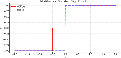
Figure 1: The plot above illustrates the comparison between the modified sign function $\widetilde{\mathop{\mathrm{sign}}}(x)(\rho=0.5)$ and the standard sign function $\mathop{\mathrm{sign}}(x)$. The $\widetilde{\mathop{\mathrm{sign}}}(x)$ function introduces a ‘dead zone’ between $-\rho$ and $\rho$ where the function value is zero, which is not present in the standard sign function. This modification effectively creates a threshold effect, only outputting non-zero values when the input $x$ exceeds the specified bounds of $\rho$ in either direction.

$$\tilde{\mathop{\mathrm{sign}}}(x)=\mathop{\mathrm{sign}}(x)\cdot\operatorname{\mathds{1}}_{\{|x|\geq\rho\}}=\begin{cases}1,&\text{ for }x\geq\rho,\\ 0,&\text{ for }-\rho<x<\rho,\\ -1,&\text{ for }x\leq-\rho.\end{cases}$$

Here, $\rho>0$ is a threshold parameter. In this context, $L^{(t)}$ is computed using a randomly sampled online batch $S_{t}$ with batch size $|S_{t}|=B$:

$$L^{(t)}=\frac{1}{B}\sum_{(\mathbf{x},y)\in S_{t}}\ell[y\cdot f(\mathbf{W}^{(t)},\mathbf{x})].$$

Consequently, the update rule for each $\mathbf{w}_{r}$ is given by:

$$\mathbf{w}_{r}^{(t+1)}=(1-\lambda\eta)\mathbf{w}_{r}^{(t)}+\eta\cdot\tilde{\mathop{\mathrm{sign}}}\bigg{(}\frac{1}{B}\sum_{(\mathbf{x},y)\in S_{t}}\sigma^{\prime}(\langle\mathbf{w}_{r}^{(t)},\mathbf{x}\rangle)\cdot a_{r}y\mathbf{x}\bigg{)},$$ (3.2)

where $\tilde{\mathop{\mathrm{sign}}}$ is applied on an elementwise basis.

Remark 3.2

The choice of sign SGD over standard SGD stems primarily from our adoption of the polynomial activation function $\sigma(z)=z^{k}$. As later explained in Section 4, this specific activation function is pivotal in constructing a neural network that accurately tackles the $k$-parity problem. However, it introduces a trade-off: the gradient’s dependency on the weights becomes polynomial rather than linear. Sign SGD addresses this issue by normalizing the gradient, ensuring that all neurons progress uniformly towards identifying the parity. Moreover, incorporating a threshold within the sign function plays a crucial role as it effectively nullifies the gradient of noisy coordinates. This, combined with regularization, aids in reducing noise, thereby enhancing the overall performance of the network.

4 Main Results

In this section, we begin by demonstrating the capability of the two-layer fully connected neural networks (3.1) to classify all samples correctly. Specifically, we construct the following good network:

$$f(\mathbf{W}^{*},\mathbf{x})=\sum_{r=1}^{2^{k}}a_{r}^{*}\sigma(\langle\mathbf{w}_{r}^{*},\mathbf{x}\rangle),$$ (4.1)

where $\big{\{}\mathbf{w}_{r,[1:k]}^{*}\big{|}r\in[2^{k}]\big{\}}=\{\pm 1\}^{k}$, $a_{r}^{*}=\prod_{j=1}^{k}\mathop{\mathrm{sign}}(w_{r,j}^{*})$ and $\mathbf{w}_{r,[k+1:d]}^{*}=\bm{0}_{d-k}$ for any $r\in[2^{k}]$. Notably, leveraging the inherent symmetry within our neural network model, we can formally assert the following proposition: $yf(\mathbf{W}^{*},\mathbf{x})=y^{\prime}f(\mathbf{W}^{*},\mathbf{x^{\prime}})$ for any $(y,\mathbf{x})$ and $(y^{\prime},\mathbf{x}^{\prime})$ generated from $\mathcal{D}_{A}$. The subsequent proposition demonstrates the precise value of the margin.

Proposition 4.1

For any data point $(\mathbf{x},y)$ generated from the distribution $\mathcal{D}_{A}$, it holds that

$$yf(\mathbf{W}^{*},\mathbf{x})=k!\cdot 2^{k}.$$ (4.2)

Proof  Given a $(y,\mathbf{x})\in\mathcal{D}_{A}$, we have that $y=\Pi_{i=1}^{k}x_{i}$. We divide the neurons into $(k+1)$ groups $\Omega_{i},i\in\{0,\ldots,k\}$. A neuron $r\in\Omega_{i}$ if and only if $\sum_{s=j}^{k}\operatorname{\mathds{1}}(\mathbf{w}_{r}^{*}=x_{j})=i$. Then we have that

$$yf(\mathbf{W}^{*},\mathbf{x}) =\sum_{r=1}^{2^{k}}(y\cdot a_{r}^{*})\cdot\sigma(\langle\mathbf{w}_{r}^{*},\mathbf{x}\rangle)$$

$$=\sum_{i=0}^{k}\sum_{r\in\Omega_{i}}(y\cdot a_{r}^{*})\cdot\sigma(\langle\mathbf{w}_{r}^{*},\mathbf{x}\rangle)$$

$$=\sum_{i=0}^{k}\sum_{r\in\Omega_{i}}\bigg{(}\prod_{j=1}^{k}\mathop{\mathrm{sign}}(x_{j})\cdot\prod_{j=1}^{k}\mathop{\mathrm{sign}}(w_{r,j}^{*})\bigg{)}\cdot\sigma(\langle\mathbf{w}_{r}^{*},\mathbf{x}\rangle)$$

$$=\sum_{i=0}^{k}{k\choose i}(-1)^{i}\sigma(k-2i)$$

$$=k!\cdot 2^{k},$$

where the third equality is due to the fact that $y=\prod_{j=1}^{k}\mathop{\mathrm{sign}}(x_{j})$ and $a_{r}^{*}=\prod_{j=1}^{k}\mathop{\mathrm{sign}}(w_{r,j}^{*})$, the fourth equality is due to the definition of $\Omega_{i}$, the last equality holds because $\sigma$ is $k$-th order polynomial activation function and Lemma E.2.  
Therefore, we can conclude that for any $(\mathbf{x},y)$, we have $yf(\mathbf{W}^{*},\mathbf{x})=k!\cdot 2^{k}>0$. We will demonstrate in the next section that training using large batch size online SGD, as long as Condition 4.2 is met, will lead to the trained neural network $f(\mathbf{W}^{(T)},\mathbf{x})$ approximating $(m/2^{k+1})\cdot f(\mathbf{W}^{*},\mathbf{x})$ effectively after $T=O(k\log(d))$ iterations. Our main theorem is based on the following conditions on the training strategy.

Condition 4.2

Suppose there exists a sufficiently large constant $C$, such that the following conditions hold:

• Neural network width $m$ satisfies $m\geq C\cdot 5^{k}\log(1/\delta)$.

• Dimension is sufficiently large: $d\geq C\log^{2}(2m/\epsilon)$.

• Online SGD batch size $B$ satisfies $B\geq C2^{k}((k-1)!)^{-2}d^{k-1}\log^{k-1}(16mdBT/\delta)\log^{2}(8mdT/\delta)$.

• Learning rate $\eta$ satisfies $\eta\leq C^{-1}$.

• Regularization parameter $\lambda$ is taken as $\lambda=1$.

• The threshold $\rho$ for the modified sign function satisfies $\rho=0.1k!$.

In the $k$-parity problem, the label $y$ is determined by a set of $k$ bits. Consequently, the total count of distinct features is $2^{k}$, reflecting all possible combinations of these bits. The condition of $m$ is established to guarantee a roughly equal number of neurons within the good neuron class, each correctly aligned with distinct features. The condition of $d$ ensures that the problem is in a sufficiently high-dimensional setting. The condition of $m,d$ implies that $d\geq\Omega(\log^{2}m)\geq\Omega(k^{2})$, which is a mild requirement for the parity $k$. In comparison, Barak et al. (2022) requires $d\geq\Omega(k^{4})$ for neural networks solving $k$-parity problem. By Stirling’s approximation, the condition of $B$ can be simplified to $B\geq\widetilde{\Omega}\big{(}k(2e\log(16mdBT/\delta)d/k^{2})^{k-1}\big{)}$. Therefore, the conditional batch size $B$ will exponentially increase as parity $k\leq O(\sqrt{d})$ goes up, which ensures that the stochastic gradient can sufficiently approximate the population gradient. Finally, the conditions of $\eta,\lambda$ ensure that gradient descent with weight decay can effectively learn the relevant features while simultaneously denoising the data. Finally, the threshold condition $\rho$ increases as parity $k$ increases to accommodate the increase of the population gradient. Based on these conditions, we give our main result on solving the parity problem in the following theorem.

Theorem 4.3

Under Condition 4.2, we run online SGD for iteration $T=\Theta\big{(}k\eta^{-1}\lambda^{-1}\log d\big{)}$ iterations. Then with probability at least $1-\delta$ we can find $\mathbf{W}^{(T)}$ such that

$$\mathbb{P}\big{(}yf(\mathbf{W}^{(T)},\mathbf{x})\geq\gamma m\big{)}\geq 1-\epsilon,$$

where $\gamma=0.25k!$ is a constant.

Theorem 4.3 establishes that, under certain conditions, a neural network is capable of learning to solve the $k$-parity problem within $\Theta(k\eta^{-1}\lambda^{-1}\log d)$ iterations, achieving a population error of at most $\epsilon$. According to Condition 4.2, the total number of samples utilized amounts to $BT=\widetilde{O}(d^{k-1})$ given a polynomial logarithmic width requirement of $m=O(1)$ with respect to $d$.

Remark 4.4

While Theorem 4.3 works for fixed second-layer training, we demonstrate that comparable results can be obtained when the second layer of the network is simultaneously trained with a lower learning rate. Detailed results and further elaboration of this aspect are provided in Appendix D. Our findings present a sample complexity of $\widetilde{O}(d^{k-1})$, aligning with Conjecture 2 posited by Abbe et al. (2023a), which suggests a sample complexity lower bound of $\tilde{\Omega}(d^{k-1})$. Besides, our results for the uniform Boolean distribution match the complexity achieved by Abbe et al. (2023a) under the isotropic Gaussian scenario. Despite these similarities in outcomes, our methodology diverges significantly: we employ online sign SGD utilizing a large batch size of $\widetilde{O}(d^{k-1})$ and conduct training over merely $\widetilde{O}(1)$ iterations. In contrast, Abbe et al. (2023a) implement projected online SGD with a minimal batch size of $1$, extending training over $\widetilde{O}(d^{k-1})$ iterations. Abbe et al. (2023a) also requires a two-phase training process for the first and second layer weights, requiring them to be trained separately.

5 Overview of Proof Technique

In this section, we discuss the main ideas used in the proof. Based on these main ideas, the proof of our main Theorem 4.3 will follow naturally. The complete proofs of all the results are given in the appendix. Section 5.1 serves as a warmup by examining population sign gradient descent. Here, three pivotal ideas crucial to the proof of stochastic sign gradient descent are introduced:

1. The impact of the initialization’s positivity or negativity on the trajectory of neuron weights.

2. The divergence between feature coordinates and noise coordinates of different neurons.

3. How a trained neural network can effectively approximate the good neural network (4.1).

Moving on to Section 5.2, we delve into the analysis of sign SGD. Contrasting with population GD, the addition in SGD analysis involves accounting for the approximation error between the population gradient and the stochastic gradient. This consideration leads to the stipulation of the batch size $B$ outlined in Condition 4.2.

5.1 Warmup: Population Gradient Descent

For population gradient, we perform the following updates:

$$\mathbf{w}_{r}^{(t+1)} =(1-\eta\lambda)\cdot\mathbf{w}_{r}^{(t)}-\eta\cdot\tilde{\mathop{\mathrm{sign}}}\big{(}\nabla_{\mathbf{w}_{r}}L_{\mathcal{D}}(\mathbf{W}^{(t)})\big{)},$$

where $L_{\mathcal{D}}(\mathbf{W})=\mathbb{E}_{(\mathbf{x},y)\sim\mathcal{D}}[\ell(y,f(\mathbf{W},\mathbf{x}))]=1-\mathbb{E}_{(\mathbf{x},y)\sim\mathcal{D}}[yf(\mathbf{W},\mathbf{x})]$. Then, the following coordinate-wise population gradient update rules hold:

$$w_{r,j}^{(t+1)} =(1-\eta\lambda)w_{r,j}^{(t)}+\eta\cdot\tilde{\mathop{\mathrm{sign}}}\Bigg{(}k!a_{r}\frac{w_{r,1}^{(t)}w_{r,2}^{(t)}\cdots w_{r,k}^{(t)}}{w_{r,j}^{(t)}}\Bigg{)}, j\in[k],$$ (5.1)

$$w_{r,j}^{(t+1)} =(1-\eta\lambda)w_{r,j}^{(t)}, j\notin[k].$$ (5.2)

In the preceding discussion of the update rule, we have identified that the noise coordinates ($j\notin[k]$) exhibit exponential decay, characterized by a decay constant of $1-\eta\lambda$. To further dissect the dynamics of this system, we turn our attention to the behavior of feature coordinates. We categorize neurons into two distinct types based on their initial alignment: a neuron is classified as a good neuron if $a_{r}=\prod_{j=1}^{k}\mathop{\mathrm{sign}}(w_{r,j}^{(0)})$, and conversely, as a bad neuron if $a_{r}=-\prod_{j=1}^{k}\mathop{\mathrm{sign}}(w_{r,j}^{(0)})$. This distinction is pivotal, as it divides the neuron population into two distinct classes: good and bad. Neurons in the good class are integral to the functionality of the final trained neural network, playing a significant role in its test accuracy. Conversely, neurons classified as bad tend to diminish in influence over the course of training, ultimately contributing minimally to the network’s overall performance. For good neurons, the update rules for feature coordinates can be reformulated to

$$\mathop{\mathrm{sign}}(w_{r,j}^{(0)})w_{r,j}^{(t+1)} =(1-\eta\lambda)\mathop{\mathrm{sign}}(w_{r,j}^{(0)})w_{r,j}^{(t)}+\eta\cdot\frac{\mathop{\mathrm{sign}}(w_{r,1}^{(0)}w_{r,1}^{(t)})\mathop{\mathrm{sign}}(w_{r,2}^{(0)}w_{r,2}^{(t)})\cdots\mathop{\mathrm{sign}}(w_{r,k}^{(0)}w_{r,k}^{(t)})}{\mathop{\mathrm{sign}}(w_{r,j}^{(0)}w_{r,j}^{(t)})}.$$ (5.3)

For neurons classified as bad, the update rules for feature coordinates can be rewritten as:

$$\mathop{\mathrm{sign}}(w_{r,j}^{(0)})w_{r,j}^{(t+1)} =(1-\eta\lambda)\mathop{\mathrm{sign}}(w_{r,j}^{(0)})w_{r,j}^{(t)}-\eta\cdot\frac{\mathop{\mathrm{sign}}(w_{r,1}^{(0)}w_{r,1}^{(t)})\mathop{\mathrm{sign}}(w_{r,2}^{(0)}w_{r,2}^{(t)})\cdots\mathop{\mathrm{sign}}(w_{r,k}^{(0)}w_{r,k}^{(t)})}{\mathop{\mathrm{sign}}(w_{r,j}^{(0)}w_{r,j}^{(t)})}.$$ (5.4)

Comparing equations (5.3) and (5.4), it becomes apparent that the feature coordinates of good and bad neurons exhibit divergent behaviors. Consequently, the feature coordinates of good neurons will significantly outweigh those of bad neurons in the long term. With the regularization parameter $\lambda$ set as $1$ in Condition 4.2, we derive the following lemma illustrating the divergent trajectories of population gradient descent for both neuron types:

Lemma 5.1

Under Condition 4.2, for good neurons $r\in\Omega_{\mathrm{g}}:=\{r\in[m]:a_{r}=\prod_{j=1}^{k}\mathop{\mathrm{sign}}(w_{r,j}^{(0)})\}$, the feature coordinates will remain the same as initialization throughout the training:

$$w_{r,j}^{(t)}=w_{r,j}^{(0)}, \forall j\in[k],t\geq 0.$$

For bad neurons $r\in\Omega_{\mathrm{b}}:=\{r\in[m]:a_{r}=-\prod_{j=1}^{k}\mathop{\mathrm{sign}}(w_{r,j}^{(0)})\}$, the feature coordinates will decay faster than noise coordiantes:

$$0<\mathop{\mathrm{sign}}(w_{r,j}^{(0)})w_{r,j}^{(t+1)}\leq(1-\eta\lambda)\mathop{\mathrm{sign}}(w_{r,j}^{(0)})w_{r,j}^{(t)}, \forall j\in[k],t\geq 0.$$

According to (5.2) and Lemma 5.1, after training $T=\Theta(k\eta^{-1}\lambda^{-1}\log(d))$ iterations, bad neurons and noise coordinates in good neurons diminish to a magnitude of $\Theta(1/\mathrm{poly}(d))$, as shown in Lemma 5.2. In contrast, the feature coordinates of good neurons remain unchanged.

Lemma 5.2

Under Condition 4.2, for $T\geq(k+1)\eta^{-1}\lambda^{-1}\log(d)$, it holds that

$$|w_{r,j}^{(T)}| \leq d^{-(k+1)}, \forall r\in\Omega_{\mathrm{g}},j\in[d]\setminus[k],$$

$$|w_{r,j}^{(T)}| \leq d^{-(k+1)}, \forall r\in\Omega_{\mathrm{b}},j\in[d].$$

This leads to the following approximation for the trained neural network:

$$f(\mathbf{W}^{(T)},\mathbf{x}) =\sum_{r=1}^{m}a_{r}\sigma(\langle\mathbf{w}_{r}^{(T)},\mathbf{x}\rangle)\approx\sum_{r\in\Omega_{\mathrm{g}}}a_{r}\sigma(\langle\mathbf{w}_{r}^{(T)},\mathbf{x}\rangle)$$

$$=\sum_{r\in\Omega_{\mathrm{g}}}\bigg{(}\prod_{j=1}^{k}\mathop{\mathrm{sign}}(w_{r,j}^{(0)})\bigg{)}\sigma(\langle\mathbf{w}_{r}^{(T)},\mathbf{x}\rangle)\approx\sum_{r\in\Omega_{\mathrm{g}}}\bigg{(}\prod_{j=1}^{k}\mathop{\mathrm{sign}}(w_{r,j}^{(0)})\bigg{)}\sigma(\langle\mathbf{w}_{r,[1:k]}^{(T)},\mathbf{x}_{[1:k]}\rangle).$$

Under Condition 4.2, the condition on $m$ ensures a balanced distribution of neurons across different initializations, approximately $m/2^{k+1}$, given $2^{k+1}$ kinds of possible initializations. This results in the trained neural network $f(\mathbf{W}^{(T)},\mathbf{x})$ closely approximating $(m/2^{k+1})\cdot f(\mathbf{W}^{*},\mathbf{x})$.

5.2 Stochastic Sign Gradient Descent

Transitioning from the trajectory trained by population gradient descent, this section delves into the dynamics under sign stochastic gradient descent (Sign SGD). We commence by presenting a lemma that estimates the approximation error between the population gradient and the stochastic gradient.

Lemma 5.3

Under Condition 4.2, with probability at least $1-\delta$ with respect to the online data generation, the stochastic gradient approximates the population gradient well:

$$\bigg{|}\frac{\partial L_{\mathcal{D}}(\mathbf{W}^{(t)})}{\partial w_{r,j}}-\frac{\partial L^{(t)}}{\partial w_{r,j}}\bigg{|}\leq\epsilon_{1}\cdot\|\mathbf{w}_{r}^{(t)}\|_{2}^{k-1}, \forall t\in[0,T],r\in[m],j\in[d],$$

where $L^{(t)}$ is the loss of randomly sampled online batch $S_{t}$ and

$$\epsilon_{1}=O(d^{-(k-1)/2}/\operatorname{\rm polylog}(d)).$$

Building upon the approximation delineated in Lemma 5.3, and considering the established order of $\rho,\epsilon_{1}$ and $\|\mathbf{w}_{r}^{(t)}\|_{2}$, we arrive at an important corollary.

Corollary 5.4

Under Condition 4.2, given the same initialization, with probability at least $1-\delta$, the stochastic sign gradient is the same as the population sign gradient:

$$\tilde{\mathop{\mathrm{sign}}}\bigg{(}\frac{\partial L_{\mathcal{D}}(\mathbf{W}^{(t)})}{\partial w_{r,j}}\bigg{)}=\tilde{\mathop{\mathrm{sign}}}\bigg{(}\frac{\partial L^{(t)}}{\partial w_{r,j}}\bigg{)}, \forall t\in[0,T],r\in[m],j\in[d].$$

This corollary suggests that, under identical initialization, the trajectory of a model trained using population gradient descent will, with high probability, align with the trajectory of a model trained using stochastic gradient descent.

6 Experiments

In this section, we present a series of experiments designed to empirically validate the theoretical results established in our main theorem. The primary objectives of these experiments are to (1) assess the test accuracy of the trained neural network, thereby corroborating the theorem’s results, and (2) verify the key lemmas concerning the behavior of good and bad neurons. Specifically, we aim to demonstrate that for good neurons, the feature coordinates remain largely unchanged from initialization while the noise coordinates decay exponentially. Conversely, for bad neurons, we expect both feature and noise coordinates to exhibit exponential decay.

Model.

We generated synthetic $k$-parity data based on Definition 3.1. Each data point $(\mathbf{x},y)$ with $\mathbf{x}\in\mathbb{R}^{d}$ and $y\in\{\pm 1\}$ is produced from distribution $\mathcal{D}_{A}$, where $A$ specifically is taken as $[k]$. We utilized two-layer fully-connected neural networks with $m$ number of neurons. The network employs a polynomial activation function $\sigma(z)=z^{k}$. The first layer weights for the $r$-th neuron, $\mathbf{w}_{r}^{(0)}\in\mathbb{R}^{d}$, were initialized following a binary scheme, where $\mathbf{w}_{r}^{(0)}\sim\text{Unif}(\{\pm 1\}^{d})$. The second layer weights for the $r$-th neuron, $a_{r}$, is randomly initialized as $1$ or $-1$ with equal probability.

Training.

Our model was trained to minimize the empirical correlation loss function, incorporating $L_{2}$ regularization with a regularization parameter set at $\lambda=1$. The training process utilized online stochastic sign gradient descent (Sign SGD) with a fixed step size $\eta$ and a predetermined batch size $B$. The principal metric for assessment was test accuracy. Our experiments were conducted considering parity $k\in\{2,3,4\}$.

For $k=2$, the model configuration included a data dimension of $d=8$, a hidden layer width of $m=12$, a total of $T=25$ epochs, a learning rate $\eta=0.1$, an online batch size of $B=64$, and a threshold for $\tilde{\mathop{\mathrm{sign}}}$ set at $\rho=0.3$. In the case of $k=3$, we employed a data dimension of $d=16$, increased the hidden layer width to $m=48$, extended the training to $T=50$ epochs, adjusted the learning rate to $\eta=0.05$, used an online batch size of $B=256$, and set the threshold for $\tilde{\mathop{\mathrm{sign}}}$ at $\rho=1$. For $k=4$, the model was further scaled up with a data dimension of $d=20$, a hidden layer width of $m=128$, a training epoch of $T=100$, a smaller learning rate of $\eta=0.02$, an online batch size of $B=2048$, and a threshold for $\tilde{\mathop{\mathrm{sign}}}$ established at $\rho=3$.

Experimental Results.

The evaluation of test accuracy across various configurations is presented in Table 3. Using neural networks with merely $2^{\Theta(k)}$ neurons, we observed high test accuracy for $k$-parity problem with $k\in\{2,3,4\}$, confirming the results of our main theorem (Theorem 4.3). These empirical results validate the efficacy of our studied model architecture (3.1) and training methodology in tackling the $k$-sparse parity problem.

To further validate our theoretical findings, we examined the change of feature and noise coordinates for the first neuron $\mathbf{w}_{1}^{(t)}$ over multiple iterations, focusing specifically on the setting $k\in\{2,3,4\}$. Figures 2, 3, 4, 5, 6, and 7 visually represent these trajectories. Our empirical findings reveal a consistent pattern: the feature coordinates ($w_{1,1}^{(t)},\ldots,w_{1,k}^{(t)}$) of the neurons identified as good (with initialization satisfying $a_{r}=\prod_{j=1}^{k}w_{r,j}^{(0)}$) exhibit relative stability, while their noise coordinates ($w_{1,k+1}^{(t)},\ldots$) show a decreasing trend over time. In contrast, the trajectories for neurons classified as bad (with initialization satisfying $a_{r}=-\prod_{j=1}^{k}w_{r,j}^{(0)}$) indicate a general reduction in all coordinate values.

These empirical observations support our theoretical analyses, as outlined in Lemma 5.1 and Lemma 5.2, showcasing the consistency between the theoretical foundations of our model and its practical performance. The disparities between good and bad neurons, as evidenced by their feature and noise coordinate behaviors, underscore the nuanced dynamics inherent in the learning process of $k$-parity problems.

$\bm{k}$	$2$	$3$	$4$
Test Accuracy (%)	$99.69\%\pm 0.29\%$	$97.75\%\pm 1.37\%$	$96.89\%\pm 0.44\%$

Table 3: Test accuracy for solving $k$-sparse parity problem with $k\in\{2,3,4\}$, averaged over 10 runs.

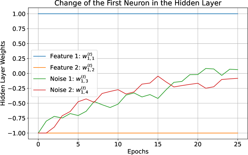
Figure 2: Illustration of a $2$-parity good neuron with initial weights $w_{1,1}^{(0)}=1$, $w_{1,2}^{(0)}=-1$, and $a_{1}=-1$.

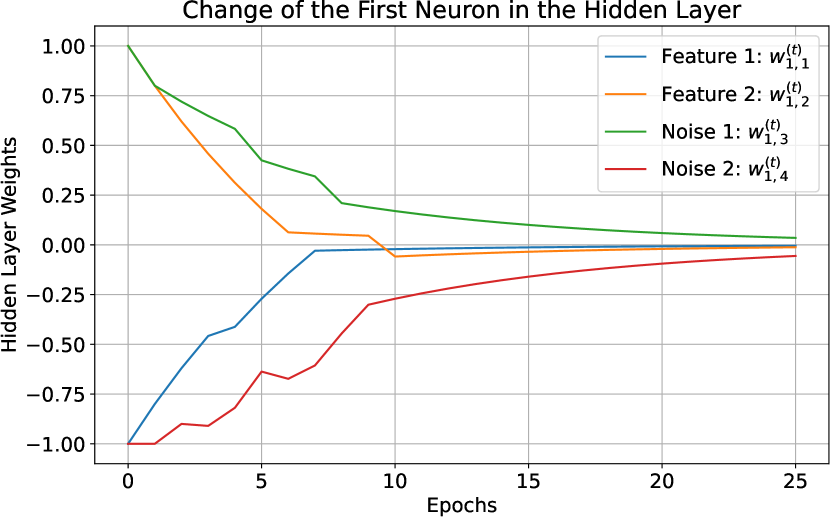
Figure 3: Illustration of a $2$-parity bad neuron with initial weights $w_{1,1}^{(0)}=-1$, $w_{1,2}^{(0)}=1$, and $a_{1}=1$.

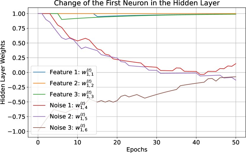
Figure 4: Illustration of a $3$-parity good neuron with initial weights $w_{1,1}^{(0)}=1$, $w_{1,2}^{(0)}=1$, $w_{1,3}^{(0)}=1$, and $a_{1}=1$.

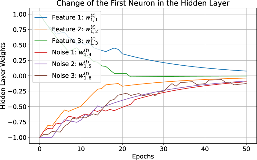
Figure 5: Illustration of a $3$-parity bad neuron with initial weights $w_{1,1}^{(0)}=1$, $w_{1,2}^{(0)}=-1$, $w_{1,3}^{(0)}=1$, and $a_{1}=1$.

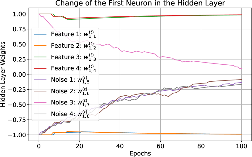
Figure 6: Illustration of a $4$-parity good neuron with initial weights $w_{1,1}^{(0)}=-1$, $w_{1,2}^{(0)}=-1$, $w_{1,3}^{(0)}=1$, $w_{1,4}^{(0)}=1$, and $a_{1}=1$.

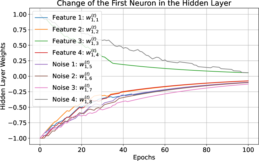
Figure 7: Illustration of a $4$-parity bad neuron with initial weights $w_{1,1}^{(0)}=-1$, $w_{1,2}^{(0)}=-1$, $w_{1,3}^{(0)}=1$, $w_{1,4}^{(0)}=-1$, and $a_{1}=-1$.

7 Conclusion and Future Work

In our study, we have conducted a detailed analysis of the $k$-parity problem, investigating how Stochastic Gradient Descent (SGD) can effectively learn intricate features from binary datasets. Our findings reveal that SGD, when employed in two-layer fully-connected neural networks solving $k$-sparse parity problem, is capable of achieving a sample complexity $\widetilde{O}(d^{k-1})$. Remarkably, this result matches the theoretical expectations set by the Statistical Query (SQ) model, underscoring the efficiency and adaptability of SGD. Our empirical evaluations further validate our theoretical results, establishing their reliability and practical relevance.

Looking ahead, an intriguing direction for future research is to explore the possibility of learning $k$-parity using SGD with even smaller queries that surpass the SQ lower bond or studying deeper neural networks. This potential advancement could pave the way for developing more efficient algorithms capable of tackling complex problems with weaker data requirements.

Appendix A Preliminary Lemmas

During the initialization phase of a neural network, neurons can be categorized into $2^{k}$ distinct groups. This classification is based on whether each feature coordinate is positive or negative. We define these groups as follows:

$$\Omega_{b_{1}b_{2}\cdots b_{k}} =\{r\in[m]\,|\,\mathop{\mathrm{sign}}(w_{r,j}^{(0)})=b_{j},\forall j\in[k]\},$$

where $b_{1},b_{2},\cdots,b_{k}\in\{\pm 1\}$. To illustrate with specific examples, consider the following special cases:

$$\Omega_{11\cdots 1} =\{r\in[m]\,|\,w_{r,j}^{(0)}>0,\forall j\in[k]\},$$

$$\Omega_{-1-1\cdots-1} =\{r\in[m]\,|\,w_{r,j}^{(0)}<0,\forall j\in[k]\}.$$

In these cases, $\Omega_{11\cdots 1}$ represents the group of neurons where all initial weights are positive across the $k$ features, while $\Omega_{-1-1\cdots-1}$ consists of neurons with all initial weights being negative. Within each group of neurons, we can further subdivide them into two subgroups based on the value of $a_{r}$. Let’s denote

$$\Omega_{\mathrm{g}}=\bigg{\{}r\in[m]\,\bigg{|}\,a_{r}=\prod_{j=1}^{k}\mathop{\mathrm{sign}}(w_{r,j}^{(0)})\bigg{\}},\Omega_{\mathrm{b}}=\bigg{\{}r\in[m]\,\bigg{|}\,a_{r}=-\prod_{j=1}^{k}\mathop{\mathrm{sign}}(w_{r,j}^{(0)})\bigg{\}},$$

where $\Omega_{g}$ denotes the good neuron set and $\Omega_{b}$ denotes the bad neuron set. We will later demonstrate in the proof and experiments that neurons in $\Omega_{\mathrm{g}}$ and neurons in $\Omega_{\mathrm{b}}$ exhibit distinct behaviors during the training process. Specifically, for neurons in $\Omega_{\mathrm{g}}$, the feature coordinates will remain largely unchanged from their initial values throughout training, while the noise coordinates will decrease to a lower order compared to the feature coordinates. On the other hand, for neurons in $\Omega_{\mathrm{b}}$, both feature coordinates and noise coordinates will decrease to a lower order compared to their initial values.

In order to establish the test error result, it is essential to impose a condition on the initialization. Specifically, the number of neurons for each type of initialization should be approximately equal.

Lemma A.1

With probability at least $1-\delta$ for the randomness in the neural network’s initialization, the sizes of the sets $\Omega_{\mathrm{g}}$ and $\Omega_{\mathrm{b}}$ are bounded as follows:

$$|\Omega_{\mathrm{g}}|,|\Omega_{\mathrm{b}}|\in[(1-\alpha)m/2,(1+\alpha)m/2].$$

Besides, the intersections of $\Omega_{b_{1}b_{2}\cdots b_{k}}$ with both $\Omega_{\mathrm{g}}$ and $\Omega_{\mathrm{b}}$ are also bounded within a specified range:

$$|\Omega_{b_{1}b_{2}\cdots b_{k}}\cap\Omega_{\mathrm{g}}|,|\Omega_{b_{1}b_{2}\cdots b_{k}}\cap\Omega_{\mathrm{b}}|\in[(1-\alpha)m/2^{k+1},(1+\alpha)m/2^{k+1}],$$

where

$$\alpha=\sqrt{\frac{3\cdot 2^{k+1}\log(2^{k+2}/\delta)}{m}}.$$

Proof Let $X_{r}=\operatorname{\mathds{1}}\big{[}w_{r,1}^{(0)}>0,\cdots,w_{r,k}^{(0)}>0,a_{r}=1\big{]}$. Then, by Chernoff bound, we have

$$\mathbb{P}\Bigg{(}\bigg{|}\sum_{r=1}^{m}X_{r}-\frac{m}{2^{k+1}}\bigg{|}\geq\alpha\cdot\frac{m}{2^{k+1}}\Bigg{)}\leq 2\exp\Big{(}-\frac{\alpha^{2}m}{3\cdot 2^{k+1}}\Big{)}.$$

Then, with probability at least $1-\delta$, we have

$$(1-\alpha)\cdot\frac{m}{2^{k+1}}\leq|\Omega_{11\cdots 1}\cap\Omega_{\mathrm{g}}|\leq(1+\alpha)\cdot\frac{m}{2^{k+1}},$$

where

$$\alpha=\sqrt{\frac{3\cdot 2^{k+1}\log(2/\delta)}{m}}.$$

By applying union bound to all $2^{k+1}$ kinds of initialization, with probability at least $1-\delta$ it holds that for any $\Omega_{b_{1}b_{2}\cdots b_{k}}\cap\Omega_{\mathrm{g}}$ and $\Omega_{b_{1}b_{2}\cdots b_{k}}\cap\Omega_{\mathrm{b}}\big{(}(b_{1},\cdots,b_{k})\in\{\pm 1\}^{k}\big{)}$

$$(1-\alpha)\cdot\frac{m}{2^{k+1}} \leq|\Omega_{b_{1}b_{2}\cdots b_{k}}\cap\Omega_{\mathrm{g}}|\leq(1+\alpha)\cdot\frac{m}{2^{k+1}},$$

$$(1-\alpha)\cdot\frac{m}{2^{k+1}} \leq|\Omega_{b_{1}b_{2}\cdots b_{k}}\cap\Omega_{\mathrm{b}}|\leq(1+\alpha)\cdot\frac{m}{2^{k+1}},$$

where

$$\alpha=\sqrt{\frac{3\cdot 2^{k+1}\log(2^{k+2}/\delta)}{m}}.$$

 

Appendix B Warmup: Population Sign GD

In this section, we train a neural network with gradient descent on the distribution $\mathcal{D}$. Here we use correlation loss function $\ell(y,\widehat{y})=1-y\widehat{y}$. Then, the loss on this attribution is $L_{\mathcal{D}}(\mathbf{W})=\mathbb{E}_{(\mathbf{x},y)\sim\mathcal{D}}[\ell(y,f(\mathbf{W},\mathbf{x}))]$, and we perform the following updates:

$$\mathbf{w}_{r}^{(t+1)} =(1-\eta\lambda)\mathbf{w}_{r}^{(t)}-\eta\cdot\widetilde{\mathop{\mathrm{sign}}}\big{(}\nabla_{\mathbf{w}_{r}}L_{\mathcal{D}}(\mathbf{W}^{(t)})\big{)}.$$

We assume the network is initialized with a symmetric initialization: for every $r\in[m]$, initialize $\mathbf{w}_{r}^{(0)}\sim\text{Unif}(\{-1,1\}^{d})$ and initialize $a_{r}\sim\text{Unif}(\{-1,1\})$.

Lemma B.1

The following coordinate-wise population sign gradient update rules hold:

$$w_{r,j}^{(t+1)} =(1-\eta\lambda)w_{r,j}^{(t)}+\eta\cdot\tilde{\mathop{\mathrm{sign}}}\Bigg{(}k!a_{r}\cdot\frac{w_{r,1}^{(t)}w_{r,2}^{(t)}\cdots w_{r,k}^{(t)}}{w_{r,j}^{(t)}}\Bigg{)}, j\in[k],$$

$$w_{r,j}^{(t+1)} =(1-\eta\lambda)w_{r,j}^{(t)}, j\notin[k].$$

Proof  For population gradient descent, we have

$$\mathbf{w}_{r}^{(t+1)} =(1-\eta\lambda)\cdot\mathbf{w}_{r}^{(t)}-\eta\cdot\tilde{\mathop{\mathrm{sign}}}\big{(}\nabla_{\mathbf{w}_{r}}L_{\mathcal{D}}(\mathbf{W})\big{)}$$

$$=(1-\eta\lambda)\cdot\mathbf{w}_{r}^{(t)}-\eta\cdot\tilde{\mathop{\mathrm{sign}}}\big{(}a_{r}\cdot\mathbb{E}_{(\mathbf{x},y)\sim\mathcal{D}}[\nabla_{\mathbf{w}_{r}}\sigma(\langle\mathbf{w}_{r}^{(t)},\mathbf{x}\rangle)]\big{)}$$

$$=(1-\eta\lambda)\cdot\mathbf{w}_{r}^{(t)}-\eta\cdot\tilde{\mathop{\mathrm{sign}}}\big{(}ka_{r}\cdot\mathbb{E}_{(\mathbf{x},y)\sim\mathcal{D}}[y\mathbf{x}(\langle\mathbf{w}_{r}^{(t)},\mathbf{x}\rangle)^{k-1}]\big{)}.$$

Notice that for $j\notin[k]$, we have

$$\mathbb{E}_{(\mathbf{x},y)\sim\mathcal{D}}[yx_{j}(\langle\mathbf{w}_{r}^{(t)},\mathbf{x}\rangle)^{k-1}] =\mathbb{E}_{(\mathbf{x},y)\sim\mathcal{D}}\bigg{[}x_{1}x_{2}\cdots x_{k}x_{j}\bigg{(}\sum_{j_{1},\cdots,j_{k-1}}w_{r,j_{1}}^{(t)}\cdots w_{r,j_{k-1}}^{(t)}x_{j_{1}}\cdots x_{j_{k-1}}\bigg{)}\bigg{]}$$

$$=\sum_{j_{1},\cdots,j_{k-1}}w_{r,j_{1}}^{(t)}\cdots w_{r,j_{k-1}}^{(t)}\cdot\mathbb{E}_{(\mathbf{x},y)\sim\mathcal{D}}\big{[}x_{1}x_{2}\cdots x_{k}x_{j}x_{j_{1}}\cdots x_{j_{k-1}}\big{]}$$

$$=0,$$

where the last equality is because $\{j_{1},\cdots,j_{k-1}\}\subsetneq\{1,\cdots,k,j\}$. This implies that

$$w_{r,j}^{(t+1)} =(1-\eta\lambda)\cdot w_{r,j}^{(t)}.$$

For $j\in[k]$, we have

$$\mathbb{E}_{(\mathbf{x},y)\sim\mathcal{D}}[yx_{j}(\langle\mathbf{w}_{r}^{(t)},\mathbf{x}\rangle)^{k-1}] =\mathbb{E}_{(\mathbf{x},y)\sim\mathcal{D}}\bigg{[}x_{1}x_{2}\cdots x_{k}x_{j}\bigg{(}\sum_{j_{1},\cdots,j_{k-1}}w_{r,j_{1}}^{(t)}\cdots w_{r,j_{k-1}}^{(t)}x_{j_{1}}\cdots x_{j_{k-1}}\bigg{)}\bigg{]}$$

$$=\sum_{j_{1},\cdots,j_{k-1}}w_{r,j_{1}}^{(t)}\cdots w_{r,j_{k-1}}^{(t)}\cdot\mathbb{E}_{(\mathbf{x},y)\sim\mathcal{D}}[x_{1}x_{2}\cdots x_{k}x_{j}x_{j_{1}}\cdots x_{j_{k-1}}]$$

$$=(k-1)!\cdot\frac{w_{r,1}^{(t)}w_{r,2}^{(t)}\cdots w_{r,k}^{(t)}}{w_{r,j}^{(t)}},$$

where the last inequality is because $\mathbb{E}_{(\mathbf{x},y)\sim\mathcal{D}}[x_{1}x_{2}\cdots x_{k}x_{j}x_{j_{1}}\cdots x_{j_{k-1}}]\neq 0$ if and only if $\{j,j_{1},\cdots,j_{k-1}\}=\{1,2,\cdots,k\}$. It follows that

$$w_{r,j}^{(t+1)} =(1-\eta\lambda)\cdot w_{r,j}^{(t)}+\eta\cdot\tilde{\mathop{\mathrm{sign}}}\Bigg{(}k!a_{r}\cdot\frac{w_{r,1}^{(t)}w_{r,2}^{(t)}\cdots w_{r,k}^{(t)}}{w_{r,j}^{(t)}}\Bigg{)}.$$

 

Given the update rules in Lemma B.1, we observe distinct behaviors for good neurons ($\Omega_{\mathrm{g}}$) and bad neurons ($\Omega_{\mathrm{b}}$). The following corollary illustrates these differences:

Corollary B.2

For any neuron $r\in\Omega_{b_{1}\cdots b_{k}}\cap\Omega_{\mathrm{g}}$, the update rule for feature coordinates $(j\in[k])$ is given by:

$$b_{j}w_{r,j}^{(t+1)} =(1-\eta\lambda)b_{j}w_{r,j}^{(t)}+\eta\cdot\frac{\mathop{\mathrm{sign}}(b_{1}w_{r,1}^{(t)})\mathop{\mathrm{sign}}(b_{2}w_{r,2}^{(t)})\cdots\mathop{\mathrm{sign}}(b_{k}w_{r,k}^{(t)})}{\mathop{\mathrm{sign}}(b_{j}w_{r,j}^{(t)})}\cdot\operatorname{\mathds{1}}\Bigg{[}\frac{|w_{r,1}^{(t)}w_{r,2}^{(t)}\cdots w_{r,k}^{(t)}|}{|w_{r,j}^{(t)}|}\geq\frac{\rho}{k!}\Bigg{]}.$$

For any neuron $r\in\Omega_{b_{1}\cdots b_{k}}\cap\Omega_{\mathrm{b}}$, the update rule for feature coordinates $(j\in[k])$ is given by:

$$b_{j}w_{r,j}^{(t+1)} =(1-\eta\lambda)b_{j}w_{r,j}^{(t)}-\eta\cdot\frac{\mathop{\mathrm{sign}}(b_{1}w_{r,1}^{(t)})\mathop{\mathrm{sign}}(b_{2}w_{r,2}^{(t)})\cdots\mathop{\mathrm{sign}}(b_{k}w_{r,k}^{(t)})}{\mathop{\mathrm{sign}}(b_{j}w_{r,j}^{(t)})}\cdot\operatorname{\mathds{1}}\Bigg{[}\frac{|w_{r,1}^{(t)}w_{r,2}^{(t)}\cdots w_{r,k}^{(t)}|}{|w_{r,j}^{(t)}|}\geq\frac{\rho}{k!}\Bigg{]}.$$

By setting the regularization parameter $\lambda$ to $1$, we observe a noteworthy property of the weight of feature coordinates in good neurons. This is formalized in the following lemma:

Lemma B.3

Assume $\lambda=1$ and $\rho<k!$. For a neuron $r\in\Omega_{b_{1}\cdots b_{k}}\cap\Omega_{\mathrm{g}}$, the weight associated with any feature coordinate remains constant across all time steps $t\geq 0$. Specifically, it holds that:

$$b_{j}w_{r,j}^{(t)}=1,\quad\forall j\in[k],\,t\geq 0.$$

Proof  We prove this by using induction. The result is obvious at $t=0$. Suppose the result holds when $t=\widetilde{t}$. Then, according to Corollary B.2, we have

$$b_{j}w_{r,j}^{(\widetilde{t}+1)} =(1-\eta\lambda)b_{j}w_{r,j}^{(\widetilde{t})}+\eta\cdot\frac{\mathop{\mathrm{sign}}(b_{1}w_{r,1}^{(\widetilde{t})})\mathop{\mathrm{sign}}(b_{2}w_{r,2}^{(\widetilde{t})})\cdots\mathop{\mathrm{sign}}(b_{k}w_{r,k}^{(\widetilde{t})})}{\mathop{\mathrm{sign}}(b_{j}w_{r,j}^{(\widetilde{t})})}\cdot\operatorname{\mathds{1}}\Bigg{[}\frac{|w_{r,1}^{(\widetilde{t})}w_{r,2}^{(\widetilde{t})}\cdots w_{r,k}^{(\widetilde{t})}|}{|w_{r,j}^{(t)}|}\geq\frac{\rho}{k!}\Bigg{]}$$

$$=(1-\eta\lambda)+\eta\cdot\operatorname{\mathds{1}}[k!\geq\rho]$$

$$=1.$$

 
The following lemma demonstrates that for bad neurons, the weights of feature coordinates tend to shrink over time. The dynamics of this shrinking are characterized as follows:

Lemma B.4

Assume $\lambda=1$ and $\eta/(1-\eta\lambda)<(\rho/k!)^{\frac{1}{k-1}}$. For a neuron $r\in\Omega_{b_{1}b_{2}\cdots b_{k}}\cap\Omega_{\mathrm{b}}$, the weights of any two feature coordinates $j$ and $j^{\prime}$ (where $j,j^{\prime}\in[k]$) are equal at any time step, that is, $b_{j}w_{r,j}^{(t)}=b_{j^{\prime}}w_{r,j^{\prime}}^{(t)}$. Furthermore, the weight of any feature coordinate $j\in[k]$ evolves according to the following inequality for any $t\geq 0$:

$$0<b_{j}w_{r,j}^{(t+1)}\leq(1-\eta\lambda)b_{j}w_{r,j}^{(t)}.$$

Proof  We prove this by using induction. We prove the following three hypotheses:

$$b_{j}w_{r,j}^{(t)}=b_{j^{\prime}}w_{r,j^{\prime}}^{(t)}, \forall j,j^{\prime}\in[k].$$ (H₁)

$$b_{j}w_{r,j}^{(t)}>0, \forall j\in[k].$$ (H₂)

$$b_{j}w_{r,j}^{(t+1)}\leq(1-\eta\lambda)b_{j}w_{r,j}^{(t)}, \forall j\in[k].$$ (H₃)

We will show that H₁$(0)$ and H₂$(0)$ are true and that for any $t\geq 0$ we have

• H₂$(t)\Longrightarrow$H₃$(t)$,

• H₁$(t)$, H₂$(t)\Longrightarrow$H₁$(t+1)$,

• H₁$(t)$, H₂$(t)\Longrightarrow$H₂$(t+1)$.

H₁$(0)$ and H₂$(0)$ are obviously true since $b_{j}w_{r,j}^{(0)}=1$ for any $j\in[k]$. Next, we prove that H₂$(t)\Longrightarrow$H₃$(t)$ and H₁$(t)$, H₂$(t)\Longrightarrow$H₁$(t+1)$. According to Corollary B.2, we have

$$b_{j}w_{r,j}^{(t+1)} =(1-\eta\lambda)b_{j}w_{r,j}^{(t)}-\eta\cdot\frac{\mathop{\mathrm{sign}}(b_{1}w_{r,1}^{(t)})\mathop{\mathrm{sign}}(b_{2}w_{r,2}^{(t)})\cdots\mathop{\mathrm{sign}}(b_{k}w_{r,k}^{(t)})}{\mathop{\mathrm{sign}}(b_{j}w_{r,j}^{(t)})}\cdot\operatorname{\mathds{1}}\Bigg{[}\frac{|w_{r,1}^{(t)}w_{r,2}^{(t)}\cdots w_{r,k}^{(t)}|}{|w_{r,j}^{(t)}|}\geq\frac{\rho}{k!}\Bigg{]}$$

$$=(1-\eta\lambda)b_{j}w_{r,j}^{(t)}-\eta\cdot\operatorname{\mathds{1}}\Bigg{[}\frac{|w_{r,1}^{(t)}w_{r,2}^{(t)}\cdots w_{r,k}^{(t)}|}{|w_{r,j}^{(t)}|}\geq\frac{\rho}{k!}\Bigg{]}$$ (B.1)

$$\leq(1-\eta\lambda)b_{j}w_{r,j}^{(t)},$$

where the second equality is by H₂$(t)$. This verifies H₃$(t)$. Besides, given H₁$(t)$, we have

$$\frac{|w_{r,1}^{(t)}w_{r,2}^{(t)}\cdots w_{r,k}^{(t)}|}{|w_{r,j}^{(t)}|}=\frac{|w_{r,1}^{(t)}w_{r,2}^{(t)}\cdots w_{r,k}^{(t)}|}{|w_{r,j^{\prime}}^{(t)}|}, \forall j,j^{\prime}\in[k].$$

Plugging this into (B.1), we can get

$$b_{j}w_{r,j}^{(t+1)}=b_{j^{\prime}}w_{r,j^{\prime}}^{(t+1)}, \forall j,j^{\prime}\in[k],$$

which verifies H₁$(t+1)$. Finally, we prove that H₁$(t)$, H₂$(t)\Longrightarrow$ H₂$(t+1)$. By (B.1) and H₁$(t)$, we have

$$b_{j}w_{r,j}^{(t+1)} =(1-\eta\lambda)b_{j}w_{r,j}^{(t)}-\eta\cdot\operatorname{\mathds{1}}\Big{[}|w_{r,j}^{(t)}|^{k-1}\geq\frac{\rho}{k!}\Big{]}.$$

If $|w_{r,j}^{(t)}|<(\rho/k!)^{\frac{1}{k-1}}$, we can get

$$b_{j}w_{r,j}^{(t+1)}=(1-\eta\lambda)b_{j}w_{r,j}^{(t)}>0.$$

If $|w_{r,j}^{(t)}|\geq(\rho/k!)^{\frac{1}{k-1}}$, given that

$$\frac{\eta}{1-\eta\lambda}<(\rho/k!)^{\frac{1}{k-1}},$$

we can get

$$b_{j}w_{r,j}^{(t+1)}=(1-\eta\lambda)b_{j}w_{r,j}^{(t)}-\eta>0.$$

 
Given Lemma B.3 and Lemma B.4, we can directly get the change of neurons of all kinds of initialization.

Corollary B.5

Assume $\lambda=1$, $\rho<k!$ and $\eta/(1-\eta\lambda)<(\rho/k!)^{\frac{1}{k-1}}$. For any fixed $(b_{1},b_{2},\cdots,b_{k})\in\{\pm 1\}^{k}$, considering $r\in\Omega_{b_{1}b_{2}\cdots b_{k}}$, we have the following statements hold.

• For any neuron $r\in\Omega_{b_{1}b_{2}\cdots b_{k}}\cap\Omega_{\mathrm{g}}$, the weights of feature coordinates remain the same as initialization: $w_{r,j}^{(t)}=b_{j}$ for any $t\geq 0$ and $j\in[k]$.

• For any neuron $r\in\Omega_{b_{1}b_{2}\cdots b_{k}}\cap\Omega_{\mathrm{b}}$, the weights of feature coordinates will shrink simultaneously over time: $b_{j}w_{r,j}^{(t)}=b_{j^{\prime}}w_{r,j^{\prime}}^{(t)}$ for any $t\geq 0$ and $j,j^{\prime}\in[k]$ and

  $$0<b_{j}w_{r,j}^{(t+1)}\leq(1-\eta\lambda)\cdot b_{j}w_{r,j}^{(t)},$$

  for any $t\geq 0$ and $j\in[k]$.

Building on Corollary B.5, we can now characterize the trajectory of all neurons over time. Specifically, after a time period $T=\Theta(k\eta^{-1}\lambda^{-1}\log(d))$, the following observations about neuron weights hold:

Lemma B.6

Assume $\lambda=1$, $\rho<k!$ and $\eta/(1-\eta\lambda)<(\rho/k!)^{\frac{1}{k-1}}$. For $T\geq(k+1)\eta^{-1}\lambda^{-1}\log d$, it holds that

$$w_{r,j}^{(T)} =b_{j}, \forall r\in\Omega_{b_{1}b_{1}\cdots b_{k}}\cap\Omega_{\mathrm{g}},j\in[k],$$

$$|w_{r,j}^{(T)}| \leq d^{-(k+1)}, \forall r\in\Omega_{\mathrm{g}},j\in[d]\setminus[k],$$

$$|w_{r,j}^{(T)}| \leq d^{-(k+1)}, \forall r\in\Omega_{\mathrm{b}},j\in[d].$$

Proof  The first equality is obvious according to Corollary B.5. We only need to prove the inequalities. According to Lemma B.1, we have for any $r\in[m]$ and $j\in[d]\setminus[k]$ that

$$|w_{r,j}^{(T)}|=(1-\eta\lambda)^{T}|w_{r,j}^{(0)}|=\big{(}(1-\eta\lambda)^{(\eta\lambda)^{-1}}\big{)}^{T\eta\lambda}\leq\exp(-T\eta\lambda)\leq d^{-(k+1)},$$

where the last inequality is by $T\geq k\eta^{-1}\lambda^{-1}\log(d)$. According to Corollary B.5, for any $r\in\Omega_{\mathrm{b}}$ and $j\in[k]$, we have that

$$|w_{r,j}^{(T)}|\leq(1-\eta\lambda)^{T}|w_{r,j}^{(0)}|=\big{(}(1-\eta\lambda)^{(\eta\lambda)^{-1}}\big{)}^{T\eta\lambda}\leq\exp(-T\eta\lambda)\leq d^{-(k+1)}.$$

 

Lemma B.7

Under Condition 4.2, with a probability of at least $1-\delta$ with respect to the randomness in the neural network’s initialization, trained neural network $f(\mathbf{W}^{(T)},\mathbf{x})$ approximates accurate classifier $(m/2^{k+1})\cdot f(\mathbf{W}^{*},\mathbf{x})$ well:

$$\mathbb{P}_{\mathbf{x}\sim\mathcal{D}_{\mathbf{x}}}\bigg{(}\frac{f(\mathbf{W}^{(T)},\mathbf{x})}{(m/2^{k+1})\cdot f(\mathbf{W}^{*},\mathbf{x})}\in[0.5,1.5]\bigg{)}\geq 1-\epsilon.$$

Proof  First, we can rewrite (4.1) as follows:

$$f(\mathbf{W}^{*},\mathbf{x}) =\sum_{(b_{1},\cdots,b_{k})\in\{\pm 1\}^{k}}(b_{1}\cdots b_{k})\cdot\sigma(\langle\mathbf{w}_{b_{1}\cdots b_{k}}^{*},\mathbf{x}\rangle),$$

where $\mathbf{w}_{b_{1}\cdots b_{k}}^{*}=[b_{1},b_{2},\cdots,b_{k},0,\cdots,0]^{\top}$. To prove this lemma, we need to estimate the noise part of the inner product $\langle\mathbf{w}_{r}^{(T)},\mathbf{x}\rangle$. By Hoeffding’s inequality, we have the following upper bound for the noise part $\sum_{j=k+1}^{d}w_{r,j}^{(T)}x_{j}$:

$$\mathbb{P}_{\mathbf{x}}\Bigg{(}\Bigg{|}\sum_{j=k+1}^{d}w_{r,j}^{(T)}x_{j}-\mathbb{E}\Bigg{[}\sum_{j=k+1}^{d}w_{r,j}^{(T)}x_{j}\Bigg{]}\Bigg{|}\geq x\Bigg{)} =\mathbb{P}_{\mathbf{x}}\Bigg{(}\Bigg{|}\sum_{j=k+1}^{d}w_{r,j}^{(t)}x_{j}\Bigg{|}\geq x\Bigg{)}$$

$$\leq 2\exp\bigg{(}-\frac{x^{2}}{2\sum_{j=k+1}^{d}[w_{r,j}^{(t)}]^{2}}\bigg{)}.$$

Then with probability at least $1-\epsilon/m$ we have that for fixed $r\in[m]$

$$\Bigg{|}\sum_{j=k+1}^{d}w_{r,j}^{(T)}x_{j}\Bigg{|} \leq\sqrt{2}\log(2m/\epsilon)\sqrt{\sum_{j=k+1}^{d}[w_{r,j}^{(T)}]^{2}}$$

$$=\sqrt{2}\log(2m/\epsilon)\|\mathbf{w}_{r,[k+1:d]}^{(T)}\|_{2}$$

$$\leq\sqrt{2}\log(2m/\epsilon)d^{-(k+1)}(d-k)^{1/2}$$

$$\leq d^{-k},$$

where the last inequality is by Condition 4.2. By applying union bound to all $m$ neurons, with probability at least $1-\epsilon$ we have that for any $r\in[m]$

$$\bigg{|}\sum_{j=k+1}^{d}w_{r,j}^{(T)}x_{j}\bigg{|}\leq d^{-k}.$$ (B.2)

By Lemma B.6, we have

$$\Big{|}f(\mathbf{W}^{(T)},\mathbf{x})-\frac{m}{2^{k+1}}\cdot f(\mathbf{W}^{*},\mathbf{x})\Big{|}$$

$$\leq\Bigg{|}\sum_{r\in\Omega_{\mathrm{g}}}a_{r}\sigma(\langle\mathbf{w}_{r}^{(T)},\mathbf{x}\rangle)-\frac{m}{2^{k+1}}\cdot\sum_{r=1}^{2^{k}}a_{r}^{*}\sigma(\langle\mathbf{w}_{r}^{*},\mathbf{x}\rangle)\Bigg{|}+\Bigg{|}\sum_{r\in\Omega_{\mathrm{b}}}a_{r}\sigma(\langle\mathbf{w}_{r}^{(T)},\mathbf{x}\rangle)\Bigg{|}$$

$$\leq\sum_{(b_{1},\cdots,b_{k})\in\{\pm 1\}^{k}}\Bigg{|}\sum_{\Omega_{b_{1}\cdots b_{k}}\cap\Omega_{\mathrm{g}}}\sigma(\langle\mathbf{w}_{r}^{(T)},\mathbf{x}\rangle)-\frac{m}{2^{k+1}}\cdot\sigma(\langle\mathbf{w}_{b_{1}\cdots b_{k}}^{*},\mathbf{x}\rangle)\Bigg{|}+\Bigg{|}\sum_{r\in\Omega_{\mathrm{b}}}a_{r}\sigma(\langle\mathbf{w}_{r}^{(T)},\mathbf{x}\rangle)\Bigg{|}$$

$$\leq\sum_{(b_{1},\cdots,b_{k})\in\{\pm 1\}^{k}}\Bigg{(}\Big{(}\frac{\alpha m}{2^{k+1}}\Big{)}\bigg{|}\sum_{j=1}^{k}b_{j}x_{j}\bigg{|}^{k}+\sum_{\Omega_{b_{1}\cdots b_{k}}\cap\Omega_{\mathrm{g}}}\big{|}\sigma(\langle\mathbf{w}_{r}^{(T)},\mathbf{x}\rangle)-\sigma(\langle\mathbf{w}_{b_{1}\cdots b_{k}}^{*},\mathbf{x}\rangle)\big{|}\Bigg{)}$$

$$\qquad+\Bigg{|}\sum_{r\in\Omega_{\mathrm{b}}}a_{r}\sigma(\langle\mathbf{w}_{r}^{(T)},\mathbf{x}\rangle)\Bigg{|}$$

$$\leq\sum_{(b_{1},\cdots,b_{k})\in\{\pm 1\}^{k}}\Bigg{(}\Big{(}\frac{\alpha m}{2^{k+1}}\Big{)}\bigg{|}\sum_{j=1}^{k}b_{j}x_{j}\bigg{|}^{k}+\sum_{\Omega_{b_{1}\cdots b_{k}}\cap\Omega_{\mathrm{g}}}kd^{-k}\big{(}k+d^{-k}\big{)}^{k-1}\Bigg{)}+|\Omega_{\mathrm{b}}|(2d^{-k}\big{)}^{k}$$

$$\leq\Big{(}\frac{\alpha m}{2^{k+1}}\Big{)}2k^{k}(1+e^{-2})^{k}+|\Omega_{\mathrm{g}}|kd^{-k}\big{(}k+d^{-k}\big{)}^{k-1}+|\Omega_{\mathrm{b}}|\big{(}2d^{-k}\big{)}^{k}$$

$$\leq\Big{(}\alpha k^{k}2^{-k}(1+e^{-2})^{k}+0.5(1+\alpha)kd^{-k}\big{(}k+d^{-k}\big{)}^{k-1}+0.5(1+\alpha)\big{(}2d^{-k}\big{)}^{k}\Big{)}\cdot m,$$

where the first three inequalities are by triangle inequality and Lemma A.1; the fourth inequality is due to

$$\big{|}\sigma(\langle\mathbf{w}_{r}^{(T)},\mathbf{x}\rangle)-\sigma(\langle\mathbf{w}_{b_{1}\cdots b_{k}}^{*},\mathbf{x}\rangle)\big{|}$$

$$\leq\big{|}(\langle\mathbf{w}_{r}^{(T)},\mathbf{x}\rangle)^{k}-(\langle\mathbf{w}_{b_{1}\cdots b_{k}}^{*},\mathbf{x}\rangle)^{k}\big{|}$$

$$\leq|\langle\mathbf{w}_{r}^{(T)},\mathbf{x}\rangle-\langle\mathbf{w}_{b_{1}\cdots b_{k}}^{*},\mathbf{x}\rangle|\cdot k(\max\{|\langle\mathbf{w}_{r}^{(T)},\mathbf{x}\rangle|,|\langle\mathbf{w}_{b_{1}\cdots b_{k}}^{*},\mathbf{x}\rangle|\})^{k-1}$$

$$=\Bigg{|}\sum_{j=k+1}^{d}w_{r,j}^{(T)}x_{j}\Bigg{|}\cdot k\Bigg{(}\max\Bigg{\{}\Bigg{|}\sum_{j=1}^{k}b_{j}x_{j}+\sum_{j=k+1}^{d}w_{r,j}^{(T)}x_{j}\Bigg{|},\Bigg{|}\sum_{j=1}^{k}b_{j}x_{j}\Bigg{|}\Bigg{\}}\Bigg{)}^{k-1}$$

$$\leq k\Bigg{|}\sum_{j=k+1}^{d}w_{r,j}^{(T)}x_{j}\Bigg{|}\cdot\Bigg{(}\Bigg{|}\sum_{j=1}^{k}b_{j}x_{j}\Bigg{|}+\Bigg{|}\sum_{j=k+1}^{d}w_{r,j}^{(T)}x_{j}\Bigg{|}\Bigg{)}^{k-1}$$

$$\leq kd^{-k}\big{(}k+d^{-k}\big{)}^{k-1}$$

by (B.2), mean value theorem and Lemma B.6 and for $r\in\Omega_{\mathrm{b}}$

$$|\sigma(\langle\mathbf{w}_{r}^{(T)},\mathbf{x}\rangle)| \leq|\langle\mathbf{w}_{r}^{(T)},\mathbf{x}\rangle|^{k}\leq\big{(}kd^{-(k+1)}+d^{-k}\big{)}^{k}\leq\big{(}2d^{-k}\big{)}^{k}.$$ (B.3)

Since $(m/2^{k+1})\cdot|f(\mathbf{W}^{*},\mathbf{x})|=0.5k!\cdot m$, then as long as

$$\alpha\leq\frac{\sqrt{2\pi k}}{8}\cdot\Big{(}\frac{e+e^{-1}}{2}\Big{)}^{-k},\text{ and }\alpha\leq 1,$$

we have

$$\frac{|f(\mathbf{W}^{(T)},\mathbf{x})-(m/2^{k+1})\cdot f(\mathbf{W}^{*},\mathbf{x})|}{(m/2^{k+1})\cdot|f(\mathbf{W}^{*},\mathbf{x})|}$$

$$\leq\frac{\alpha k^{k}2^{-k}(1+e^{-2})^{k}+0.5(1+\alpha)kd^{-k}\big{(}k+d^{-k}\big{)}^{k-1}+0.5(1+\alpha)\big{(}2d^{-k}\big{)}^{k}}{0.5k!}$$

$$\leq\frac{2\alpha k^{k}2^{-k}(1+e^{-2})^{k}+(1+\alpha)kd^{-k}\big{(}k+d^{-k}\big{)}^{k-1}+(1+\alpha)\big{(}2d^{-k}\big{)}^{k}}{\sqrt{2\pi k}(k/e)^{k}}$$

$$=\sqrt{\frac{2}{\pi k}}\alpha\Big{(}\frac{e+e^{-1}}{2}\Big{)}^{k}+\sqrt{\frac{2}{\pi k}}\cdot\bigg{(}1+\frac{d^{-k}}{k}\bigg{)}^{k-1}\cdot\Big{(}\frac{e}{d}\Big{)}^{k}+\sqrt{\frac{2}{\pi k}}\cdot\Big{(}\frac{2e}{kd^{k}}\Big{)}^{k}$$

$$\leq 0.5,$$

where the second inequality is by Stirling’s approximation. Then it follows that

$$\frac{f(\mathbf{W}^{(T)},\mathbf{x})}{(m/2^{k+1})\cdot f(\mathbf{W}^{*},\mathbf{x})}\in[0.5,1.5].$$

 

Appendix C Stochastic Sign GD

In this section, we consider stochastic sign gradient descent for learning $k$-parity function. The primary aim of this section is to demonstrate that the trajectory produced by SGD closely resembles that of population GD. To begin, let’s recall the update rule of SGD:

$$\mathbf{w}_{r}^{(t+1)} =(1-\lambda\eta)\mathbf{w}_{r}^{(t)}+\eta\cdot\tilde{\mathop{\mathrm{sign}}}\bigg{(}\frac{1}{|S_{t}|}\sum_{(\mathbf{x},y)\in S_{t}}\sigma^{\prime}(\langle\mathbf{w}_{r}^{(t)},\mathbf{x}\rangle)\cdot a_{r}y\mathbf{x}\bigg{)},$$

where $|S_{t}|=B$. Our initial step involves estimating the approximation error between the stochastic gradient and the population gradient, detailed within the lemma that follows.

Lemma C.1

With probability at least $1-\delta$ with respect to the randomness of online data selection, for all $t\leq T$, the following bound holds true for each neuron $r\in[m]$ and for each coordinate $j\in[d]$:

$$\Bigg{|}\frac{1}{|S_{t}|}\sum_{(\mathbf{x},y)\in S_{t}}\sigma^{\prime}(\langle\mathbf{w}_{r}^{(t)},\mathbf{x}\rangle)\cdot a_{r}y\mathbf{x}-\mathbb{E}_{(\mathbf{x},y)}\big{[}\sigma^{\prime}(\langle\mathbf{w}_{r}^{(t)},\mathbf{x}\rangle)\cdot a_{r}yx_{j}\big{]}\Bigg{|}\leq\epsilon_{1}\cdot\|\mathbf{w}_{r}^{(t)}\|_{2}^{k-1},$$ (C.1)

where $\epsilon_{1}$ is defined as

$$\epsilon_{1} =\frac{2^{k/2}k(\log(16mdBT/\delta))^{(k-1)/2}\log(8mdT/\delta)}{\sqrt{B}}+\frac{kd^{(k-3)/2}\delta}{8mBT}.$$

Proof  To prove (C.1), let us introduce the following notations:

$$g_{r,j}(\mathbf{x},y) =\sigma^{\prime}(\langle\mathbf{w}_{r}^{(t)},\mathbf{x}\rangle)\cdot a_{r}yx_{j}=k(\langle\mathbf{w}_{r}^{(t)},\mathbf{x}\rangle)^{k-1}\cdot a_{r}yx_{j},$$

$$h_{r,j}(\mathbf{x},y) =g_{r,j}(\mathbf{x},y)\cdot\operatorname{\mathds{1}}\big{[}|\langle\mathbf{w}_{r}^{(t)},\mathbf{x}\rangle|\leq\gamma\big{]},$$

where $g_{r,j}(\mathbf{x},y)$ represents the gradient at the point $(\mathbf{x},y)$, and $h_{r,j}(\mathbf{x},y)$ denotes the truncated version of $g_{r,j}(\mathbf{x},y)$, which is employed for the convenience of applying the Hoeffding’s inequality. Firstly, utilizing Hoeffding’s inequality, we can assert the following:

$$\mathbb{P}\Bigg{(}\Bigg{|}\frac{1}{B}\sum_{(\mathbf{x},y)\in S_{t}}h_{r,j}(\mathbf{x},y)-\mathbb{E}_{(\mathbf{x},y)\sim\mathcal{D}}h_{r,j}(\mathbf{x},y)\Bigg{|}\geq x\Bigg{)}\leq 2\exp\Bigg{(}-\frac{Bx^{2}}{2(k\gamma^{k-1})^{2}}\Bigg{)}.$$ (C.2)

Furthermore, we can establish an upper bound for the difference between the expectations of $h_{r,j}(\mathbf{x},y)$ and $g_{r,j}(\mathbf{x},y)$:

$$\Big{|}\mathbb{E}_{(\mathbf{x},y)\sim\mathcal{D}}h_{r,j}(\mathbf{x},y)-\mathbb{E}_{(\mathbf{x},y)\sim\mathcal{D}}g_{r,j}(\mathbf{x},y)\Big{|} =\Big{|}\mathbb{E}_{(\mathbf{x},y)\sim\mathcal{D}}g_{r,j}(\mathbf{x},y)\cdot\operatorname{\mathds{1}}\big{[}|\langle\mathbf{w}_{r}^{(t)},\mathbf{x}\rangle|>\gamma\big{]}\Big{|}$$ (C.3)

$$\leq kd^{(k-1)/2}\|\mathbf{w}_{r}^{(t)}\|_{2}^{k-1}\cdot\mathbb{P}\big{(}|\langle\mathbf{w}_{r}^{(t)},\mathbf{x}\rangle|>\gamma\big{)}$$

$$\leq kd^{(k-1)/2}\|\mathbf{w}_{r}^{(t)}\|_{2}^{k-1}\cdot 2\exp\bigg{(}-\frac{\gamma^{2}}{2\|\mathbf{w}_{r}^{(t)}\|_{2}^{2}}\bigg{)},$$

where the first inequality is by Cauchy inequality and the second inequality is by Hoeffding’s inequality. Additionally, with high probability, the gradient and the truncated gradient are identical:

$$\mathbb{P}\Bigg{(}\Bigg{|}\frac{1}{B}\sum_{(\mathbf{x},y)\in S_{t}}h_{r,j}(\mathbf{x},y)-\frac{1}{B}\sum_{(\mathbf{x},y)\in S_{t}}g_{r,j}(\mathbf{x},y)\Bigg{|}=0\Bigg{)}$$ (C.4)

$$=\mathbb{P}\Bigg{(}\Bigg{|}\frac{1}{B}\sum_{(\mathbf{x},y)\in S_{t}}g_{r,j}(\mathbf{x},y)\operatorname{\mathds{1}}\big{[}|\langle\mathbf{w}_{r}^{(t)},\mathbf{x}\rangle|>\gamma\big{]}\Bigg{|}=0\Bigg{)}$$

$$\geq\mathbb{P}\Big{(}|\langle\mathbf{w}_{r}^{(t)},\mathbf{x}\rangle|\leq\gamma,\forall(\mathbf{x},y)\in S_{t}\Big{)}$$

$$\geq\Bigg{(}1-2\exp\bigg{(}-\frac{\gamma^{2}}{2\|\mathbf{w}_{r}^{(t)}\|_{2}^{2}}\bigg{)}\Bigg{)}^{B}$$

$$\geq 1-2B\exp\bigg{(}-\frac{\gamma^{2}}{2\|\mathbf{w}_{r}^{(t)}\|_{2}^{2}}\bigg{)},$$

where the second inequality applies Hoeffding’s inequality. Combining inequalities (C.2), (C.3), and (C.4), we can assert with probability at least

$$1-2\exp\bigg{(}-\frac{Bx^{2}}{2(k\gamma^{k-1})^{2}}\bigg{)}-2B\exp\bigg{(}-\frac{\gamma^{2}}{2\|\mathbf{w}_{r}^{(t)}\|_{2}^{2}}\bigg{)}$$ (C.5)

that the following inequality holds:

$$\Bigg{|}\frac{1}{B}\sum_{(\mathbf{x},y)\in S_{t}}g_{r,j}(\mathbf{x},y)-\mathbb{E}_{(\mathbf{x},y)\sim\mathcal{D}}g_{r,j}(\mathbf{x},y)\Bigg{|}\leq x+kd^{(k-1)/2}\|\mathbf{w}_{r}^{(t)}\|_{2}^{k-1}\cdot 2\exp\bigg{(}-\frac{\gamma^{2}}{2\|\mathbf{w}_{r}^{(t)}\|_{2}^{2}}\bigg{)}.$$ (C.6)

By setting $\gamma=\sqrt{2\log(16B/\delta)}\|\mathbf{w}_{r}^{(t)}\|_{2}$ and $x=\sqrt{2}k\gamma^{k-1}\log(8/\delta)/\sqrt{B}$, we establish that with probability at least $1-\delta$, the following bound is true:

$$\Bigg{|}\frac{1}{B}\sum_{(\mathbf{x},y)\in S_{t}}g_{r,j}(\mathbf{x},y)-\mathbb{E}_{(\mathbf{x},y)\sim\mathcal{D}}g_{r,j}(\mathbf{x},y)\Bigg{|}$$

$$\leq\frac{\sqrt{2}k\gamma^{k-1}\log(8/\delta)}{\sqrt{B}}+\frac{kd^{(k-1)/2}\|\mathbf{w}_{r}^{(t)}\|_{2}^{k-1}\delta}{8B}$$

$$=\frac{2^{k/2}k(\log(16B/\delta))^{(k-1)/2}\log(8/\delta)\|\mathbf{w}_{r}^{(t)}\|_{2}^{k-1}}{\sqrt{B}}+\frac{kd^{(k-1)/2}\|\mathbf{w}_{r}^{(t)}\|_{2}^{k-1}\delta}{8B}.$$

Applying a union bound over all indices $r\in[m],j\in[d]$, and iterations $t\in[0,T-1]$, we conclude with probability at least $1-\delta$ that

$$\Bigg{|}\frac{1}{B}\sum_{(\mathbf{x},y)\in S_{t}}g_{r,j}(\mathbf{x},y)-\mathbb{E}_{(\mathbf{x},y)\sim\mathcal{D}}g_{r,j}(\mathbf{x},y)\Bigg{|}$$

$$=\frac{2^{k/2}k(\log(16mdBT/\delta))^{(k-1)/2}\log(8mdT/\delta)\|\mathbf{w}_{r}^{(t)}\|_{2}^{k-1}}{\sqrt{B}}+\frac{kd^{(k-1)/2}\|\mathbf{w}_{r}^{(t)}\|_{2}^{k-1}\delta}{8mdBT}$$

$$=\Bigg{(}\frac{2^{k/2}k(\log(16mdBT/\delta))^{(k-1)/2}\log(8mdT/\delta)}{\sqrt{B}}+\frac{kd^{(k-3)/2}\delta}{8mBT}\Bigg{)}\cdot\|\mathbf{w}_{r}^{(t)}\|_{2}^{k-1}.$$

 
Based on Lemma C.1, we can get the following lemma showing that with high probability, the stochastic sign gradient follows the same update rule as the population sign gradient.

Lemma C.2

Under Condition 4.2, with probability at least $1-\delta$ with respect to the randomness of online data selection, the following sign SGD update rule holds:

$$w_{r,j}^{(t+1)} =(1-\eta\lambda)w_{r,j}^{(t)}+\eta\cdot\tilde{\mathop{\mathrm{sign}}}\Bigg{(}k!a_{r}\cdot\frac{w_{r,1}^{(t)}w_{r,2}^{(t)}\cdots w_{r,k}^{(t)}}{w_{r,j}^{(t)}}\Bigg{)}, j\in[k],$$

$$w_{r,j}^{(t+1)} =(1-\eta\lambda)w_{r,j}^{(t)}, j\notin[k].$$

Proof  We prove this by using induction. We prove the following hypotheses:

$$\|\mathbf{w}_{r}^{(t+1)}\|_{2}\leq\|\mathbf{w}_{r}^{(t)}\|_{2}, \forall r\in[m].$$ (H₁)

$$w_{r,j}^{(t+1)}=(1-\eta\lambda)w_{r,j}^{(t)}+\eta\cdot\tilde{\mathop{\mathrm{sign}}}\Bigg{(}k!a_{r}\cdot\frac{w_{r,1}^{(t)}w_{r,2}^{(t)}\cdots w_{r,k}^{(t)}}{w_{r,j}^{(t)}}\Bigg{)}, \forall r\in[m],j\in[k].$$ (H₂)

$$w_{r,j}^{(t+1)}=(1-\eta\lambda)w_{r,j}^{(t)}, \forall r\in[m],j\notin[k].$$ (H₃)

$$b_{j}w_{r,j}^{(t)}=1, \forall r\in\Omega_{b_{1}\cdots b_{k}}\cap\Omega_{\mathrm{g}},\forall j\in[k].$$ (H₄)

$$b_{j}w_{r,j}^{(t)}=b_{j^{\prime}}w_{r,j^{\prime}}^{(t)}, \forall r\in\Omega_{b_{1}b_{2}\cdots b_{k}}\cap\Omega_{\mathrm{g}},\forall j,j^{\prime}\in[k].$$ (H₅)

$$0<b_{j}w_{r,j}^{(t+1)}\leq(1-\eta\lambda)b_{j}w_{r,j}^{(t)}, \forall r\in\Omega_{b_{1}b_{2}\cdots b_{k}}\cap\Omega_{\mathrm{b}},\forall j\in[k].$$ (H₆)

We will show that H₂$(0)$, H₃$(0)$, H₄$(0)$ and H₅$(0)$ are true and for any $t\geq 0$ we have

• H₂$(t)$, H₄$(t)$ $\Longrightarrow$ H₄$(t+1)$. (This can be established by adapting the proof of Lemma B.3; hence, we omit the proof details here.)

• H₂$(t)$, H₅$(t)$ $\Longrightarrow$ H₅$(t+1)$, H₆$(t)$. (This can be shown by following the proof of Lemma B.4, so the proof details are omitted here.)

• H₃$(t)$, H₄$(t)$, H₄$(t+1)$, H₆$(t)$ $\Longrightarrow$H₁$(t)$.

• $\{$H₁$(s)\}_{s=0}^{t}$ $\Longrightarrow$ H₂$(t+1)$, H₃$(t+1)$.

H₄$(0)$ and H₅$(0)$ are obviously true since $w_{r,j}^{(0)}=b_{j}$ for any $r\in\Omega_{b_{1}b_{2}\cdots b_{k}}$ and $j\in[k]$. To prove that H₂$(0)$ and H₃$(0)$ are true, we only need to verify that

$$\tilde{\mathop{\mathrm{sign}}}\Bigg{(}\frac{1}{|S_{0}|}\sum_{(\mathbf{x},y)\in S_{0}}\sigma^{\prime}(\langle\mathbf{w}_{r}^{(0)},\mathbf{x}\rangle)\cdot a_{r}yx_{j}\Bigg{)} =\tilde{\mathop{\mathrm{sign}}}\Bigg{(}k!a_{r}\cdot\frac{w_{r,1}^{(0)}w_{r,2}^{(0)}\cdots w_{r,k}^{(0)}}{w_{r,j}^{(0)}}\Bigg{)}, \forall j\in[k],$$ (C.7)

$$\tilde{\mathop{\mathrm{sign}}}\Bigg{(}\frac{1}{|S_{0}|}\sum_{(\mathbf{x},y)\in S_{0}}\sigma^{\prime}(\langle\mathbf{w}_{r}^{(0)},\mathbf{x}\rangle)\cdot a_{r}yx_{j}\Bigg{)} =0, \forall j\notin[k].$$ (C.8)

By Lemma C.1, we have for $j\notin[k]$

$$\Bigg{|}\frac{1}{|S_{0}|}\sum_{(\mathbf{x},y)\in S_{t}}\sigma^{\prime}(\langle\mathbf{w}_{r}^{(0)},\mathbf{x}\rangle)\cdot a_{r}yx_{j}\Bigg{|} \leq\epsilon_{1}\cdot\|\mathbf{w}_{r}^{(0)}\|_{2}^{k-1}=\epsilon_{1}\cdot d^{\frac{k-1}{2}}<\rho,$$

leading to (C.8). For $j\in[k]$, we have

$$\Bigg{|}\frac{1}{|S_{0}|}\sum_{(\mathbf{x},y)\in S_{0}}\sigma^{\prime}(\langle\mathbf{w}_{r}^{(0)},\mathbf{x}\rangle)\cdot a_{r}yx_{j}-k!a_{r}\cdot\frac{w_{r,1}^{(0)}w_{r,2}^{(0)}\cdots w_{r,k}^{(0)}}{w_{r,j}^{(0)}}\Bigg{|} \leq\epsilon_{1}\cdot\|\mathbf{w}_{r}^{(0)}\|_{2}^{k-1}=\epsilon_{1}\cdot d^{\frac{k-1}{2}},$$

Since $k!-\epsilon_{1}\cdot d^{\frac{k-1}{2}}\geq\rho$, we can get

$$\tilde{\mathop{\mathrm{sign}}}\Bigg{(}\frac{1}{|S_{0}|}\sum_{(\mathbf{x},y)\in S_{0}}\sigma^{\prime}(\langle\mathbf{w}_{r}^{(0)},\mathbf{x}\rangle)\cdot a_{r}yx_{j}\Bigg{)} =\tilde{\mathop{\mathrm{sign}}}\Bigg{(}k!a_{r}\cdot\frac{w_{r,1}^{(0)}w_{r,2}^{(0)}\cdots w_{r,k}^{(0)}}{w_{r,j}^{(0)}}\Bigg{)},$$

which verifies (C.7). Next, we verify that H₃$(t)$, H₄$(t)$, H₄$(t+1)$, H₆$(t)$ $\Longrightarrow$H₁$(t)$. For $r\in\Omega_{\mathrm{g}}$, given H₃$(t)$, H₄$(t)$ and H₄$(t+1)$, we can get

$$\|\mathbf{w}_{r}^{(t+1)}\|_{2} =\Bigg{(}\sum_{j=1}^{d}\big{(}w_{r,j}^{(t+1)}\big{)}^{2}\Bigg{)}^{\frac{1}{2}}=\Bigg{(}\sum_{j=1}^{k}\big{(}w_{r,j}^{(t)}\big{)}^{2}+\sum_{j=k+1}^{d}\big{(}(1-\eta\lambda)w_{r,j}^{(t)}\big{)}^{2}\Bigg{)}^{\frac{1}{2}}\leq\|\mathbf{w}_{r}^{(t)}\|_{2}.$$

For $r\in\Omega_{\mathrm{b}}$, given H₃$(t)$ and H₆$(t)$, we can get

$$\|\mathbf{w}_{r}^{(t+1)}\|_{2} =\Bigg{(}\sum_{j=1}^{d}\big{(}w_{r,j}^{(t+1)}\big{)}^{2}\Bigg{)}^{\frac{1}{2}}\leq\Bigg{(}\sum_{j=1}^{d}\big{(}(1-\eta\lambda)w_{r,j}^{(t)}\big{)}^{2}\Bigg{)}^{\frac{1}{2}}\leq\|\mathbf{w}_{r}^{(t)}\|_{2}.$$

Finally, we verify that $\{$H₁$(s)\}_{s=0}^{t}$ $\Longrightarrow$ H₂$(t+1)$, H₃$(t+1)$. Notice that $\|\mathbf{w}_{r}^{(t+1)}\|_{2}\leq\|\mathbf{w}_{r}^{(0)}\|_{2}$ given $\{$H₁$(s)\}_{s=0}^{t}$, we can prove H₃$(t+1)$ and H₂$(t+1)$ by following the prove of (C.7) and (C.8) given Lemma C.1.  
Based on Lemma C.2 and the proof of Lemma B.6, Lemma B.7, we can get the following lemmas and theorems aligning with the result of population sign GD.

Lemma C.3

Under Condition 4.2, for $T=\Theta(k\eta^{-1}\lambda^{-1}\log(d))$,with a probability of at least $1-\delta$ with respect to the randomness of the online data selection, it holds that

$$w_{r,j}^{(T)} =b_{j}, \forall r\in\Omega_{b_{1}b_{1}\cdots b_{k}}\cap\Omega_{\mathrm{g}},j\in[k],$$

$$|w_{r,j}^{(T)}| \leq d^{-(k+1)}, \forall r\in\Omega_{\mathrm{g}},j\in[d]\setminus[k],$$

$$|w_{r,j}^{(T)}| \leq d^{-(k+1)}, \forall r\in\Omega_{\mathrm{b}},j\in[d].$$

Lemma C.4

Under Condition 4.2, with a probability of at least $1-2\delta$ with respect to the randomness in the neural network’s initialization and the online data selection, trained neural network $f(\mathbf{W}^{(T)},\mathbf{x})$ approximates accurate classifier $(m/2^{k+1})\cdot f(\mathbf{W}^{*},\mathbf{x})$ well:

$$\mathbb{P}_{\mathbf{x}\sim\mathcal{D}_{\mathbf{x}}}\bigg{(}\frac{f(\mathbf{W}^{(T)},\mathbf{x})}{(m/2^{k+1})\cdot f(\mathbf{W}^{*},\mathbf{x})}\in[0.5,1.5]\bigg{)}\geq 1-\epsilon.$$

Based on Lemma C.4, we are now ready to prove our main theorem.

Theorem C.5

Under Condition 4.2, we run mini-batch SGD for $T=\Theta(k\eta^{-1}\lambda^{-1}\log(d))$ iterations. Then with probability at least $1-2\delta$ with respect to the randomness of neural network initialization and the online data selection, it holds that

$$\mathbb{P}_{(\mathbf{x},y)\sim\mathcal{D}}(yf(\mathbf{W}^{(T)},\mathbf{x})\geq\gamma m)\geq 1-\epsilon.$$

where $\gamma=0.25k!$ is a constant.

Proof  Given Lemma C.4, we have

$$\mathbb{P}_{\mathbf{x}\sim\mathcal{D}_{\mathbf{x}}}\bigg{(}\frac{f(\mathbf{W}^{(T)},\mathbf{x})}{(m/2^{k+1})\cdot f(\mathbf{W}^{*},\mathbf{x})}\geq 0.5\bigg{)}$$

$$\geq\mathbb{P}_{\mathbf{x}\sim\mathcal{D}_{\mathbf{x}}}\bigg{(}\frac{f(\mathbf{W}^{(T)},\mathbf{x})}{(m/2^{k+1})\cdot f(\mathbf{W}^{*},\mathbf{x})}\in[0.5,1.5]\bigg{)}$$

$$\geq 1-\epsilon.$$

According to Proposition 4.1, we can get

$$\mathbb{P}_{\mathbf{x}\sim\mathcal{D}_{\mathbf{x}}}\bigg{(}\frac{f(\mathbf{W}^{(T)},\mathbf{x})}{(m/2^{k+1})\cdot f(\mathbf{W}^{*},\mathbf{x})}\geq 0.5\bigg{)}$$

$$=\mathbb{P}_{\mathbf{x}\sim\mathcal{D}_{\mathbf{x}}}\bigg{(}\frac{yf(\mathbf{W}^{(T)},\mathbf{x})}{(m/2^{k+1})\cdot k!\cdot 2^{k}}\geq 0.5\bigg{)}$$

$$=\mathbb{P}_{\mathbf{x}\sim\mathcal{D}_{\mathbf{x}}}\big{(}yf(\mathbf{W}^{(T)},\mathbf{x})\geq 0.25k!\cdot m\big{)},$$

which completes the proof.  

Appendix D Trainable Second Layer

In this section, we consider sign SGD for training the first and second layers together. In this scenario, we have the following sign SGD update rule:

$$\mathbf{w}_{r}^{(t+1)} =(1-\lambda\eta)\mathbf{w}_{r}^{(t)}+\eta\cdot\tilde{\mathop{\mathrm{sign}}}\bigg{(}\frac{1}{|S_{t}|}\sum_{(\mathbf{x},y)\in S_{t}}\sigma^{\prime}(\langle\mathbf{w}_{r}^{(t)},\mathbf{x}\rangle)\cdot a_{r}^{(t)}y\mathbf{x}\bigg{)},$$ (D.1)

$$a_{r}^{(t+1)} =a_{r}^{(t)}+\eta_{2}\cdot\tilde{\mathop{\mathrm{sign}}}\bigg{(}\frac{1}{|S_{t}|}\sum_{(\mathbf{x},y)\in S_{t}}\sigma(\langle\mathbf{w}_{r}^{(t)},\mathbf{x}\rangle)\bigg{)},$$ (D.2)

where $|S_{t}|=B$. For training the neural network over $T=\Theta(k(\eta\lambda)^{-1}\log(d))$ iterations, we adopt a small learning rate for the second layer, adhering to the condition:

$$\eta_{2}\leq\frac{1}{4T}\sqrt{\frac{\pi k}{8}}\Big{(}\frac{e+e^{-1}}{2}\Big{)}^{-k}.$$

The network is initialized symmetrically: for every $r\in[m]$, initialize $\mathbf{w}_{r}^{(0)}\sim\text{Unif}(\{-1,1\}^{d})$ and initialize $a_{r}^{(0)}\sim\text{Unif}(\{-1,1\})$. Under this setting, denote

$$\Omega_{\mathrm{g}}=\bigg{\{}r\in[m]\,\bigg{|}\,a_{r}=\prod_{j=1}^{k}\mathop{\mathrm{sign}}(w_{r,j}^{(0)})\bigg{\}},\Omega_{\mathrm{b}}=\bigg{\{}r\in[m]\,\bigg{|}\,a_{r}=-\prod_{j=1}^{k}\mathop{\mathrm{sign}}(w_{r,j}^{(0)})\bigg{\}}.$$

Similar to the fix-second-layer case, our initial step involves estimating the approximation error between the SGD gradient and the population gradient, detailed within the lemma that follows.

Lemma D.1

With probability at least $1-\delta$ with respect to the randomness of online data selection, for all $t\leq T$, we have for any $r\in[m]$ and $j\in[d]$ that

$$\Bigg{|}\frac{1}{|S_{t}|}\sum_{(\mathbf{x},y)\in S_{t}}\sigma^{\prime}(\langle\mathbf{w}_{r}^{(t)},\mathbf{x}\rangle)\cdot a_{r}^{(t)}yx_{j}-\mathbb{E}\big{[}\sigma^{\prime}(\langle\mathbf{w}_{r}^{(t)},\mathbf{x}\rangle)\cdot a_{r}^{(t)}yx_{j}\big{]}\Bigg{|} \leq\epsilon_{1}\cdot|a_{r}^{(t)}|\|\mathbf{w}_{r}^{(t)}\|_{2}^{k-1},$$ (D.3)

where

$$\epsilon_{1} =\frac{2^{k/2}k(\log(16mdBT/\delta))^{(k-1)/2}\log(8mdT/\delta)}{\sqrt{B}}+\frac{kd^{(k-3)/2}\delta}{8mBT}.$$

Proof  To prove (D.3), we denote

$$g_{r,j}(\mathbf{x},y) =\sigma^{\prime}(\langle\mathbf{w}_{r}^{(t)},\mathbf{x}\rangle)\cdot a_{r}^{(t)}yx_{j}=k(\langle\mathbf{w}_{r}^{(t)},\mathbf{x}\rangle)^{k-1}\cdot a_{r}^{(t)}yx_{j},$$

$$h_{r,j}(\mathbf{x},y) =g_{r,j}(\mathbf{x},y)\cdot\operatorname{\mathds{1}}\big{[}|\langle\mathbf{w}_{r}^{(t)},\mathbf{x}\rangle|\leq\gamma\big{]}.$$

Initially, by invoking Hoeffding’s inequality, we have the following probability bound:

$$\mathbb{P}\Bigg{(}\Bigg{|}\frac{1}{B}\sum_{(\mathbf{x},y)\in S_{t}}h_{r,j}(\mathbf{x},y)-\mathbb{E}_{(\mathbf{x},y)\sim\mathcal{D}}h_{r,j}(\mathbf{x},y)\Bigg{|}\geq x\Bigg{)}\leq 2\exp\Bigg{(}-\frac{Bx^{2}}{2(k\gamma^{k-1}a_{r}^{(t)})^{2}}\Bigg{)}.$$ (D.4)

Next, we establish an upper bound for the difference between the expected values of $h_{r,j}(\mathbf{x},y)$ and $g_{r,j}(\mathbf{x},y)$:

$$\Big{|}\mathbb{E}_{(\mathbf{x},y)\sim\mathcal{D}}h_{r,j}(\mathbf{x},y)-\mathbb{E}_{(\mathbf{x},y)\sim\mathcal{D}}g_{r,j}(\mathbf{x},y)\Big{|} =\Big{|}\mathbb{E}_{(\mathbf{x},y)\sim\mathcal{D}}g_{r,j}(\mathbf{x},y)\cdot\operatorname{\mathds{1}}\big{[}|\langle\mathbf{w}_{r}^{(t)},\mathbf{x}\rangle|>\gamma\big{]}\Big{|}$$ (D.5)

$$\leq kd^{(k-1)/2}\|\mathbf{w}_{r}^{(t)}\|_{2}^{k-1}|a_{r}^{(t)}|\cdot\mathbb{P}\big{(}|\langle\mathbf{w}_{r}^{(t)},\mathbf{x}\rangle|>\gamma\big{)}$$

$$\leq kd^{(k-1)/2}\|\mathbf{w}_{r}^{(t)}\|_{2}^{k-1}|a_{r}^{(t)}|\cdot 2\exp\bigg{(}-\frac{\gamma^{2}}{2\|\mathbf{w}_{r}^{(t)}\|_{2}^{2}}\bigg{)},$$

where the first inequality follows from the Cauchy-Schwarz inequality and the second from Hoeffding’s inequality. With high probability, the gradient and the truncated gradient coincide:

$$\mathbb{P}\Bigg{(}\Bigg{|}\frac{1}{B}\sum_{(\mathbf{x},y)\in S_{t}}h_{r,j}(\mathbf{x},y)-\frac{1}{B}\sum_{(\mathbf{x},y)\in S_{t}}g_{r,j}(\mathbf{x},y)\Bigg{|}=0\Bigg{)}$$ (D.6)

$$=\mathbb{P}\Bigg{(}\Bigg{|}\frac{1}{B}\sum_{(\mathbf{x},y)\in S_{t}}g_{r,j}(\mathbf{x},y)\operatorname{\mathds{1}}\big{[}|\langle\mathbf{w}_{r}^{(t)},\mathbf{x}\rangle|>\gamma\big{]}\Bigg{|}=0\Bigg{)}$$

$$\geq\mathbb{P}\Big{(}|\langle\mathbf{w}_{r}^{(t)},\mathbf{x}\rangle|\leq\gamma,\forall(\mathbf{x},y)\in S_{t}\Big{)}$$

$$\geq\Bigg{(}1-2\exp\bigg{(}-\frac{\gamma^{2}}{2\|\mathbf{w}_{r}^{(t)}\|_{2}^{2}}\bigg{)}\Bigg{)}^{B}$$

$$\geq 1-2B\exp\bigg{(}-\frac{\gamma^{2}}{2\|\mathbf{w}_{r}^{(t)}\|_{2}^{2}}\bigg{)}.$$

Combing (D.4), (D.5) and (D.6), it holds with probability at least

$$1-2\exp\Big{(}-\frac{Bx^{2}}{2(k\gamma^{k-1}a_{r}^{(t)})^{2}}\Big{)}-2B\exp\bigg{(}-\frac{\gamma^{2}}{2\|\mathbf{w}_{r}^{(t)}\|_{2}^{2}}\bigg{)}$$

that

$$\Bigg{|}\frac{1}{B}\sum_{(\mathbf{x},y)\in S_{t}}g_{r,j}(\mathbf{x},y)-\mathbb{E}_{(\mathbf{x},y)\sim\mathcal{D}}g_{r,j}(\mathbf{x},y)\Bigg{|}\leq x+kd^{(k-1)/2}\|\mathbf{w}_{r}^{(t)}\|_{2}^{k-1}|a_{r}^{(t)}|\cdot 2\exp\bigg{(}-\frac{\gamma^{2}}{2\|\mathbf{w}_{r}^{(t)}\|_{2}^{2}}\bigg{)}.$$

By taking $\gamma=\sqrt{2\log(16B/\delta)}\|\mathbf{w}_{r}^{(t)}\|_{2}$ and $x=\sqrt{2}k\gamma^{k-1}|a_{r}^{(t)}|\log(8/\delta)/\sqrt{B}$, then with probability at least $1-\delta$ it holds that

$$\Bigg{|}\frac{1}{B}\sum_{(\mathbf{x},y)\in S_{t}}g_{r,j}(\mathbf{x},y)-\mathbb{E}_{(\mathbf{x},y)\sim\mathcal{D}}g_{r,j}(\mathbf{x},y)\Bigg{|}$$

$$\leq\frac{\sqrt{2}k\gamma^{k-1}|a_{r}^{(t)}|\log(8/\delta)}{\sqrt{B}}+\frac{kd^{(k-1)/2}\|\mathbf{w}_{r}^{(t)}\|_{2}^{k-1}|a_{r}^{(t)}|\delta}{8B}$$

$$=\frac{2^{k/2}k(\log(16B/\delta))^{(k-1)/2}\log(8/\delta)|a_{r}^{(t)}|\|\mathbf{w}_{r}^{(t)}\|_{2}^{k-1}}{\sqrt{B}}+\frac{kd^{(k-1)/2}|a_{r}^{(t)}|\|\mathbf{w}_{r}^{(t)}\|_{2}^{k-1}\delta}{8B}.$$

Then, by applying a union bound to all $r\in[m],j\in[d]$ and iterations $t\in[0,T-1]$, it holds with probability at least $1-\delta$ that

$$\Bigg{|}\frac{1}{B}\sum_{(\mathbf{x},y)\in S_{t}}g_{r,j}(\mathbf{x},y)-\mathbb{E}_{(\mathbf{x},y)\sim\mathcal{D}}g_{r,j}(\mathbf{x},y)\Bigg{|}$$

$$=\frac{2^{k/2}k(\log(16mdBT/\delta))^{(k-1)/2}\log(8mdT/\delta)\|\mathbf{w}_{r}^{(t)}\|_{2}^{k-1}|a_{r}^{(t)}|}{\sqrt{B}}+\frac{kd^{(k-1)/2}\|\mathbf{w}_{r}^{(t)}\|_{2}^{k-1}|a_{r}^{(t)}|\delta}{8mdBT}$$

$$=\Bigg{(}\frac{2^{k/2}k(\log(16mdBT/\delta))^{(k-1)/2}\log(8mdT/\delta)}{\sqrt{B}}+\frac{kd^{(k-3)/2}\delta}{8mBT}\Bigg{)}\cdot|a_{r}^{(t)}|\|\mathbf{w}_{r}^{(t)}\|_{2}^{k-1}.$$

 

Lemma D.2 (Stability of Second Layer Weights)

For $t\leq T=\Theta(k(\eta\lambda)^{-1}\log(d))$, the magnitude of change in the second layer weights from their initial values is bounded as follows:

$$|a_{r}^{(t)}-a_{r}^{(0)}| \leq c,$$

where

$$c=\frac{1}{4}\sqrt{\frac{\pi k}{8}}\Big{(}\frac{e+e^{-1}}{2}\Big{)}^{-k}.$$

Consequently, the sign of each weight remains consistent over time:

$$\mathop{\mathrm{sign}}(a_{r}^{(t)})=\mathop{\mathrm{sign}}(a_{r}^{(0)}).$$

Proof  Notice that by (D.2) and $\tilde{\mathop{\mathrm{sign}}}(\cdot)\in\{-1,0,1\}$, we can get for any $t\geq 0$ that

$$a_{r}^{(t)}-\eta_{2}\leq a_{r}^{(t+1)}\leq a_{r}^{(t)}+\eta_{2},$$

which implies that

$$|a_{r}^{(t)}-a_{r}^{(0)}| \leq\eta_{2}t\leq\eta_{2}T\leq c,$$

where the second inequality is by $t\leq T$, and the last inequality is by the condition $\eta_{2}\leq\frac{1}{4T}\sqrt{\frac{\pi k}{8}}\Big{(}\frac{e+e^{-1}}{2}\Big{)}^{-k}$.  

Lemma D.3

With probability at least $1-\delta$ with respect to the randomness of online data selection, the following sign SGD update rule holds:

$$w_{r,j}^{(t+1)} =(1-\eta\lambda)w_{r,j}^{(t)}+\eta\cdot\tilde{\mathop{\mathrm{sign}}}\Bigg{(}k!a_{r}^{(t)}\cdot\frac{w_{r,1}^{(t)}w_{r,2}^{(t)}\cdots w_{r,k}^{(t)}}{w_{r,j}^{(t)}}\Bigg{)}, j\in[k],$$

$$w_{r,j}^{(t+1)} =(1-\eta\lambda)w_{r,j}^{(t)}, j\notin[k].$$

Proof  We prove this by using induction. We prove the following hypotheses:

$$\|\mathbf{w}_{r}^{(t+1)}\|_{2}\leq\|\mathbf{w}_{r}^{(t)}\|_{2}, \forall r\in[m].$$ (H₁)

$$w_{r,j}^{(t+1)}=(1-\eta\lambda)w_{r,j}^{(t)}+\eta_{1}\cdot\tilde{\mathop{\mathrm{sign}}}\Bigg{(}k!a_{r}^{(t)}\cdot\frac{w_{r,1}^{(t)}w_{r,2}^{(t)}\cdots w_{r,k}^{(t)}}{w_{r,j}^{(t)}}\Bigg{)}, \forall r\in[m],j\in[k].$$ (H₂)

$$w_{r,j}^{(t+1)}=(1-\eta\lambda)w_{r,j}^{(t)}, \forall r\in[m],j\notin[k].$$ (H₃)

$$b_{j}w_{r,j}^{(t)}=1, \forall r\in\Omega_{b_{1}\cdots b_{k}}\cap\Omega_{\mathrm{g}},\forall j\in[k].$$ (H₄)

$$b_{j}w_{r,j}^{(t)}=b_{j^{\prime}}w_{r,j^{\prime}}^{(t)}, \forall r\in\Omega_{b_{1}b_{2}\cdots b_{k}}\cap\Omega_{\mathrm{g}},\forall j,j^{\prime}\in[k].$$ (H₅)

$$0<b_{j}w_{r,j}^{(t+1)}\leq(1-\eta\lambda)b_{j}w_{r,j}^{(t)}, \forall r\in\Omega_{b_{1}b_{2}\cdots b_{k}}\cap\Omega_{\mathrm{b}},\forall j\in[k].$$ (H₆)

We will show that H₂$(0)$, H₃$(0)$, H₄$(0)$ and H₅$(0)$ are true and for any $t\geq 0$ we have

• H₂$(t)$, H₄$(t)$ $\Longrightarrow$ H₄$(t+1)$.

• H₂$(t)$, H₅$(t)$ $\Longrightarrow$ H₅$(t+1)$, H₆$(t)$.

• H₃$(t)$, H₄$(t)$, H₄$(t+1)$, H₆$(t)$ $\Longrightarrow$H₁$(t)$.

• $\{$H₁$(s)\}_{s=0}^{t}$ $\Longrightarrow$ H₂$(t+1)$, H₃$(t+1)$.

H₄$(0)$ and H₅$(0)$ are obviously true since $w_{r,j}^{(0)}=b_{j}$ for any $r\in\Omega_{b_{1}b_{2}\cdots b_{k}}$ and $j\in[k]$. To prove that H₂$(0)$ and H₃$(0)$ are true, we can follow the proof of Lemma C.2 by noticing that $|a_{r}^{(0)}|=1$. Now, we verify that H₂$(t)$, H₄$(t)$ $\Longrightarrow$ H₄$(t+1)$. By H₂$(t)$ and $\mathop{\mathrm{sign}}(a_{r}^{(t)})=\mathop{\mathrm{sign}}(a_{r}^{(0)})$ according to Lemma D.2, we have for any neuron $r\in\Omega_{b_{1}b_{2}\cdots b_{k}}\cap\Omega_{\mathrm{g}}$ that

$$b_{j}w_{r,j}^{(t+1)} =(1-\eta\lambda)b_{j}w_{r,j}^{(t)}$$

$$\qquad+\eta\cdot\frac{\mathop{\mathrm{sign}}(b_{1}w_{r,1}^{(t)})\mathop{\mathrm{sign}}(b_{2}w_{r,2}^{(t)})\cdots\mathop{\mathrm{sign}}(b_{k}w_{r,k}^{(t)})}{\mathop{\mathrm{sign}}(b_{j}w_{r,j}^{(t)})}\cdot\operatorname{\mathds{1}}\Bigg{[}\frac{|a_{r}^{(0)}w_{r,1}^{(t)}w_{r,2}^{(t)}\cdots w_{r,k}^{(t)}|}{|w_{r,j}^{(t)}|}\geq\frac{\rho}{k!}\Bigg{]}$$

$$=(1-\eta\lambda)+\eta\cdot\operatorname{\mathds{1}}[k!\geq\rho]$$

$$=1,$$

where the last equality is by $\rho\leq k!(1-c)\leq k!\cdot|a_{r}^{(t)}|$. H₂$(t)$, H₅$(t)$ $\Longrightarrow$ H₅$(t+1)$, H₆$(t)$ can be verified in the same way as Lemma B.4 by noticing that $\rho\leq k!(1-c)\leq k!\cdot|a_{r}^{(t)}|$. H₃$(t)$, H₄$(t)$, H₄$(t+1)$, H₆$(t)$ $\Longrightarrow$H₁$(t)$ can be proved by following exactly the same proof as Lemma B.4. $\{$H₁$(s)\}_{s=0}^{t}$ $\Longrightarrow$ H₂$(t+1)$, H₃$(t+1)$ be verified in the same way as Lemma B.4 by noticing that $\epsilon_{1}\cdot(1+c)\cdot d^{\frac{k-1}{2}}<\rho$ and $k!-\epsilon_{1}\cdot(1+c)\cdot d^{\frac{k-1}{2}}>\rho$.  
Based on Lemma D.2 and Lemma D.3, we can get the following lemmas and theorems aligning with the result of the fixed second-layer case.

Lemma D.4

For $T=\Theta(k\eta^{-1}\lambda^{-1}\log(d))$,with a probability of at least $1-\delta$ with respect to the randomness of the online data selection, it holds that

$$w_{r,j}^{(T)} =b_{j}, \forall r\in\Omega_{b_{1}b_{1}\cdots b_{k}}\cap\Omega_{\mathrm{g}},j\in[k],$$

$$|w_{r,j}^{(T)}| \leq d^{-(k+1)}, \forall r\in\Omega_{\mathrm{g}},j\in[d]\setminus[k],$$

$$|w_{r,j}^{(T)}| \leq d^{-(k+1)}, \forall r\in\Omega_{\mathrm{b}},j\in[d].$$

Lemma D.5

With a probability of at least $1-2\delta$ with respect to the randomness in the neural network’s initialization and the online data selection, trained neural network $f(\mathbf{W}^{(T)},\mathbf{x})$ approximates accurate classifier $(m/2^{k+1})\cdot f(\mathbf{W}^{*},\mathbf{x})$ well:

$$\mathbb{P}_{\mathbf{x}\sim\mathcal{D}_{\mathbf{x}}}\bigg{(}\frac{f(\mathbf{W}^{(T)},\mathbf{x})}{(m/2^{k+1})\cdot f(\mathbf{W}^{*},\mathbf{x})}\in[0.25,1.75]\bigg{)}\geq 1-\epsilon.$$

Proof  Let

$$\widetilde{f}(\mathbf{W}^{(T)},\mathbf{x})=\sum_{r=1}^{m}a_{r}^{(0)}\cdot\sigma(\langle\mathbf{w}_{r}^{(T)},\mathbf{x}\rangle).$$

By the proof of Lemma B.7, we can get

$$\frac{|\widetilde{f}(\mathbf{W}^{(T)},\mathbf{x})-(m/2^{k+1})\cdot f(\mathbf{W}^{*},\mathbf{x})|}{(m/2^{k+1})\cdot|f(\mathbf{W}^{*},\mathbf{x})|}\leq 0.5.$$

To prove the result, we need to estimate the difference between $\widetilde{f}(\mathbf{W}^{(T)},\mathbf{x})$ and $f(\mathbf{W}^{(T)},\mathbf{x})$:

$$\big{|}f(\mathbf{W}^{(T)},\mathbf{x})-\widetilde{f}(\mathbf{W}^{(T)},\mathbf{x})\big{|} =\Bigg{|}\sum_{r=1}^{m}(a_{r}^{(T)}-a_{r}^{(0)})\cdot\sigma(\langle\mathbf{w}_{r}^{(T)},\mathbf{x}\rangle)\Bigg{|}$$ (D.7)

$$\leq\sum_{r=1}^{m}|a_{r}^{(T)}-a_{r}^{(0)}|\cdot|\langle\mathbf{w}_{r}^{(T)},\mathbf{x}\rangle|^{k}$$

$$\leq c\sum_{r=1}^{m}|\langle\mathbf{w}_{r}^{(T)},\mathbf{x}\rangle|^{k}$$

$$=c\underbrace{\sum_{r\in\Omega_{\mathrm{g}}}|\langle\mathbf{w}_{r}^{(T)},\mathbf{x}\rangle|^{k}}_{I_{1}}+c\underbrace{\sum_{r\in\Omega_{\mathrm{b}}}|\langle\mathbf{w}_{r}^{(T)},\mathbf{x}\rangle|^{k}}_{I_{2}}$$

where the first inequality is by triangle inequality; the second inequality is by Lemma D.2. Then, we provide upper bounds for terms $I_{1}$ and $I_{2}$ respectively. For $I_{1}$, we have the following upper bound:

$$I_{1} =\sum_{r\in\Omega_{\mathrm{g}}}|\langle\mathbf{w}_{r,[1:k]}^{(T)},\mathbf{x}_{[1:k]}\rangle+\langle\mathbf{w}_{r,[k+1:d]}^{(T)},\mathbf{x}_{[k+1:d]}\rangle|^{k}$$

$$\leq\sum_{r\in\Omega_{\mathrm{g}}}|\langle\mathbf{w}_{r,[1:k]}^{(T)},\mathbf{x}_{[1:k]}\rangle|^{k}+\sum_{r\in\Omega_{\mathrm{g}}}|\langle\mathbf{w}_{r,[k+1:d]}^{(T)},\mathbf{x}_{[k+1:d]}\rangle|\cdot k\big{(}|\langle\mathbf{w}_{r,[1:k]}^{(T)},\mathbf{x}_{[1:k]}\rangle|+|\langle\mathbf{w}_{r,[k+1:d]}^{(T)},\mathbf{x}_{[k+1:d]}\rangle|\big{)}^{k}$$

$$\leq\sum_{(b_{1},\cdots,b_{k})\in\{\pm 1\}^{k}}\sum_{r\in\Omega_{b_{1}b_{2}\cdots b_{k}}\cap\Omega_{\mathrm{g}}}\bigg{|}\sum_{j=1}^{k}b_{j}x_{j}\bigg{|}^{k}+\sum_{r\in\Omega_{\mathrm{g}}}d^{-k}\cdot k\big{(}k+d^{-k}\big{)}^{k}$$

$$\leq\sum_{(b_{1},\cdots,b_{k})\in\{\pm 1\}^{k}}\Big{(}\frac{1+\alpha}{2^{k+1}}\Big{)}m\cdot\bigg{|}\sum_{j=1}^{k}b_{j}x_{j}\bigg{|}^{k}+\Big{(}\frac{1+\alpha}{2}\Big{)}m\cdot d^{-k}\cdot k\big{(}k+d^{-k}\big{)}^{k}$$

$$\leq\Big{(}\frac{1+\alpha}{2^{k+1}}\Big{)}m\cdot 2k^{k}(1+e^{-2})^{k}+\Big{(}\frac{1+\alpha}{2}\Big{)}m\cdot d^{-k}\cdot k\big{(}k+d^{-k}\big{)}^{k},$$ (D.8)

where the first inequality is by mean value theorem; the second inequality is by (B.2) and Lemma D.4; the third inequality is by Lemma A.1; the last inequality is by Lemma E.3. For $I_{2}$, we have the following upper bound

$$I_{2} \leq|\Omega_{\mathrm{b}}|\cdot(2d^{-k})^{k}\leq\Big{(}\frac{1+\alpha}{2}\Big{)}m\cdot(2d^{-k})^{k}.$$ (D.9)

By plugging (D.8) and (D.9) into (D.7), we can get:

$$\big{|}f(\mathbf{W}^{(T)},\mathbf{x})-\widetilde{f}(\mathbf{W}^{(T)},\mathbf{x})\big{|}$$

$$\leq c\big{(}(1+\alpha)2^{-k}m\cdot k^{k}(1+e^{-2})^{k}+0.5(1+\alpha)m\cdot d^{-k}\cdot k\big{(}k+d^{-k}\big{)}^{k}+0.5(1+\alpha)m\cdot(2d^{-k})^{k}\big{)}.$$

Therefore, we have

$$\frac{\big{|}f(\mathbf{W}^{(T)},\mathbf{x})-\widetilde{f}(\mathbf{W}^{(T)},\mathbf{x})\big{|}}{(m/2^{k+1})\cdot|f(\mathbf{W}^{*},\mathbf{x})|}$$

$$\leq c\cdot\frac{(1+\alpha)2^{-k}m\cdot k^{k}(1+e^{-2})^{k}+0.5(1+\alpha)m\cdot d^{-k}\cdot k\big{(}k+d^{-k}\big{)}^{k}+0.5(1+\alpha)m\cdot(2d^{-k})^{k}}{0.5k!\cdot m}$$

$$\leq c\cdot\frac{2(1+\alpha)2^{-k}\cdot k^{k}(1+e^{-2})^{k}+(1+\alpha)\cdot d^{-k}\cdot k\big{(}k+d^{-k}\big{)}^{k}+(1+\alpha)\cdot(2d^{-k})^{k}}{\sqrt{2\pi k}(k/e)^{k}}$$

$$=c\cdot\Bigg{(}\sqrt{\frac{2}{\pi k}}(1+\alpha)\Big{(}\frac{e+e^{-1}}{2}\Big{)}^{k}+\sqrt{\frac{2}{\pi k}}\cdot\bigg{(}1+\frac{d^{-k}}{k}\bigg{)}^{k-1}\cdot\Big{(}\frac{e}{d}\Big{)}^{k}+\sqrt{\frac{2}{\pi k}}\cdot\Big{(}\frac{2e}{kd^{k}}\Big{)}^{k}\Bigg{)}$$

$$\leq c\cdot\sqrt{\frac{8}{\pi k}}\Big{(}\frac{e+e^{-1}}{2}\Big{)}^{k}$$

$$=\frac{1}{4},$$

where the second inequality is by Stirling’s approximation, and the last equality is due to $c=\frac{1}{4}\sqrt{\frac{\pi k}{8}}\big{(}\frac{e+e^{-1}}{2}\big{)}^{-k}$.  

Appendix E Auxiliary Lemmas

We first introduce a finite difference operator with step $h$ and order $n$ as follows,

$$\Delta^{n}_{h}[f](x)=\sum_{i=0}^{n}{k\choose i}(-1)^{n-i}f(x+ih).$$

The following Lemma calculates the value finite difference operating on the polynomial function.

Lemma E.1

(Milne-Thomson, 2000) For $f(x)=x^{n}$, we have that $\Delta^{n}_{h}[f](x)=h^{n}n!$.

Based on Lemma E.1, we have the following Lemma, which calculates the margin of good NNs defined in (3.1).

Lemma E.2

For any integer $k$, we have

$$\sum_{i=0}^{k}{k\choose i}(-1)^{i}(k-2i)^{k}=2^{k}k!.$$ (E.1)

Proof  Applying Lemma E.1 with $f(x)=x^{k}$, $n=k$ in Lemma E.1 gives,

$$\sum_{i=0}^{k}{k\choose i}(-1)^{i}(k-2i)^{k}=(-1)^{k}\Delta^{k}_{-2}[f](k)=(-1)^{k}(-2)^{k}k!=2^{k}k!,$$

where the first equality is due to the definition of finite difference operator and the last equality is due to Lemma E.1.  

Lemma E.3

For any positive integer $k$, it holds that

$$\sum_{i=0}^{k}{k\choose i}|k-2i|^{k}\leq 2k^{k}(1+e^{-2})^{k}.$$

Proof We can establish the following inequality:

$$\sum_{i=0}^{k}{k\choose i}|k-2i|^{k} \leq 2\sum_{i=0}^{\lfloor\frac{k-1}{2}\rfloor}{k\choose i}|k-2i|^{k}$$

$$=2k^{k}\sum_{i=0}^{\lfloor\frac{k-1}{2}\rfloor}{k\choose i}\Big{(}1-\frac{2i}{k}\Big{)}^{k}$$

$$\leq 2k^{k}\sum_{i=0}^{\lfloor\frac{k-1}{2}\rfloor}{k\choose i}\exp(-2i)$$

$$\leq 2k^{k}\sum_{i=0}^{k}{k\choose i}\exp(-2i)$$

$$=2k^{k}(1+e^{-2})^{k},$$

where the first inequality is by ${k\choose i}={k\choose k-i}$, the second inequality is by $1-t\leq\exp(-t),\forall t\in\mathbb{R}$, the last inequality is by ${k\choose i}\exp(-2i)>0$.