Information theory unifies atomistic machine learning, uncertainty quantification, and materials thermodynamics

Abstract

An accurate description of information is relevant for a range of problems in atomistic modeling, such as sampling methods, detecting rare events, analyzing datasets, or performing uncertainty quantification (UQ) in machine learning (ML)-driven simulations. Although individual methods have been proposed for each of these tasks, they lack a common theoretical background integrating their solutions. Here, we introduce an information theoretical framework that unifies predictions of phase transformations, kinetic events, dataset optimality, and model-free UQ from atomistic simulations, thus bridging materials modeling, ML, and statistical mechanics. We first demonstrate that, for a proposed representation, the information entropy of a distribution of atom-centered environments is a surrogate value for thermodynamic entropy. Using molecular dynamics (MD) simulations, we show that information entropy differences from trajectories can be used to build phase diagrams, identify rare events, and recover classical theories of nucleation. Building on these results, we use this general concept of entropy to quantify information in datasets for ML interatomic potentials (IPs), informing compression, explaining trends in testing errors, and evaluating the efficiency of active learning strategies. Finally, we propose a model-free UQ method for MLIPs using information entropy, showing it reliably detects extrapolation regimes, scales to millions of atoms, and goes beyond model errors. This method is made available as the package QUESTS: Quick Uncertainty and Entropy via STructural Similarity, providing a new unifying theory for data-driven atomistic modeling and combining efforts in ML, first-principles thermodynamics, and simulations.

I Introduction

Information is a fundamental concept in science that brings unifying views in a range of fields, from thermodynamics¹ and communication theory ² to deep learning.³ Specifically within statistical thermodynamics, the concept of information relates to the number of microstates accessible by a macrostate and is often referred to as “entropy”. Along with the internal energy and other state variables, entropy connects the microscropic description of a system, such as fluctuations in atomic positions, to its macroscopic properties, such as phase stability or heat capacity. The parallels between thermodynamic entropy and information theory² have motivated quantitative descriptions of thermodynamic entropy by analyzing information contents from simulations, though this has proven challenging.^{4, 5, 6, 7, 8, 9, 10, 11, 12, 13} Connecting information and thermodynamic entropies often requires an explicit definition of the degrees of freedom for the system, such as pair distribution functions,^{14, 15, 10} motion coordinates^{4, 8} or displacements around known lattice sites¹³ in addition to correction factors. In principle, the entropy can be computed exactly for systems such as liquids,^{14, 15} where many-body expansions of correlation functions fully approximate the entropy due to spatial arrangement of particles. More generally, however, this hand-crafted approach, along with combinatorial configurational spaces and expensive free energy estimation methods, hinders the computation of entropy within atomistic simulations and lowers the fidelity of ab initio materials thermodynamics.

In a related field, the use of hand-crafted features was influential in classical interatomic potentials (IPs), where explicit functional forms define energy functions for certain terms.^{16, 17} In the context of atomistic data and simulations, machine learning interatomic potentials (MLIPs) often exhibit better accuracy and versatility than their classical counterparts^{18, 19, 20, 21, 22, 23, 24, 25, 26, 27, 28} and do not require a predefined functional form as adopted in the latter.^{16, 17} Particularly with neural network (NN) potentials, many-body interactions can be approximated by decomposing the total energy into site-centered energies that can be predicted from localized symmetry functions.¹⁸ Although this strategy has greatly improved the development of new MLIPs, the black-box behavior of several ML models hinders their use in extrapolation regimes where little to no information about an atomic environment is present in the training domain.^{29, 30, 31} Thus, understanding the information contents within datasets is not only essential for thermodynamic analysis, but also for improving training efficiency, robustness, and uncertainty quantification (UQ) methods within atomistic ML.

In this work, we propose a theory that connects information entropy and thermodynamic entropy differences in the context of atomistic data and simulations. By proposing a unified view of atomistic information theory, we show that the information entropy from a distribution of local descriptors predicts thermodynamic entropy differences, detects and recovers classical theories of nucleation, explains trends in MLIP errors, rationalizes dataset analysis/compression, and provides a robust UQ estimate for ML-driven simulations in a number of exemplar applications. First, when compared against entropies obtained with the thermodynamic integration method, our method correctly estimates entropy differences across a range of volumes and temperatures for the phase transition between $\alpha$ and $\beta$ tin and the phase transition between face-centered cubic (FCC) and body-centered cubic (BCC) copper at high temperatures and pressures. Then, by building on this connection between information and thermodynamic entropy, we show that the method further can be used to explain rare events, recovering results from classical nucleation theory from a simple information analysis and quantifying entropies along transformation pathways. Using theorems from information entropy, we additionally apply our method to analyze datasets for MLIPs, analyzing their completeness, compressing them based on their maximum entropy, and explaining trends in test errors reported in the literature. Finally, we use conditional information values to perform UQ without relying on models, demonstrating the robustness of our metric and its use in detecting failed simulations. In all examples, we show how information contents can be used to obtain unexpected physical insights from atomistic datasets, including alternative analyses for critical nuclei or correlations in error metrics for datasets. This work provides an unifying view on atomistic thermodynamics, dataset construction, and UQ, and can be extended to enable faster and more accurate materials modeling beyond predictions of potential energy surfaces.

II Results

II.1 Connecting atomistic representations to information entropy

To approximate a one-to-one mapping between atomistic environments and data distributions, we propose a descriptor for atomic environments inspired by recent studies in continuous and bijective representations of crystalline structures³² and similar to the DeepMD descriptors.²³ Given their success in a range of applications,^{23, 33} the representation offers a rich metric space without sacrificing its computational efficiency. This simplified representation allows us to perform non-parametric estimates of data distributions even in extremely large datasets. To obtain the descriptor, we begin by sorting the distances from a central atom $i$ to its $k$-nearest neighbors (within periodic boundary conditions, if appropriate) and obtain a vector $\mathbf{X}_{i}^{(1)}$ with length $k$,

$$\mathbf{X}_{i}^{(1)}=\begin{bmatrix}\frac{w(r_{i1})}{r_{i1}}&\ldots&\frac{w(r_{ik})}{r_{ik}}\end{bmatrix}^{T},~{}r_{ij}\leq r_{i(j+1)},$$ (1)

with $1\leq j\leq k$ due to the $k$-nearest neighbors approach and $w$ a smooth cutoff function given by

$$w(r)=\begin{cases}\left[1-\left(\frac{r}{r_{c}}\right)^{2}\right]^{2},&0\leq r\leq r_{c},\\ 0,&r>r_{c}.\end{cases}$$ (2)

However, the radial distances alone do not capture bond angles and cannot be used to fully reconstruct the environment, so we construct a second vector to augment $\mathbf{X}_{i}^{(1)}$ that aggregates distances from neighboring atoms, inspired by the Weisfeiler-Lehman isomorphism test and analogous to message-passing schemes in graph neural networks (see LABEL:sec:methods and Fig. S1),

$$X_{in}^{(2)}=\left\langle\frac{\sqrt{w(r_{ij})w(r_{il})}}{r_{jl}}\right\rangle_{n},~{}j,l\in\mathcal{N}(i),~{}X_{in}\geq X_{i(n+1)},$$ (3)

where $j$ and $l$ are atoms in the neighborhood $\mathcal{N}$ of atom $i$, $\langle.\rangle_{n}$ represents the arithmetic mean between the $n$-th elements of the sequence (details in the LABEL:sec:stext), and $1\leq n\leq k-1$ due to the number of $k$-nearest neighbors pairs. The final descriptor $\mathbf{X}_{i}$ is obtained by concatenating $\mathbf{X}_{i}^{(1)}$ and $\mathbf{X}_{i}^{(2)}$. Furthermore, as this representation requires only the computation of a neighbor list, it can be easily parallelized and scaled to large systems.

To quantify the information entropy from a distribution of feature vectors $\{\mathbf{X}\}$, we start from the definition of the Shannon entropy $\mathcal{H}$,²

$$\mathcal{H}\left[p(x)\right]=-\int p(x)\log p(x)dx,$$ (4)

where $\log$ is the natural logarithm, implying that $\mathcal{H}$ is measured in units of nats. Given a kernel $K_{h}$ with bandwidth $h$, we can perform a kernel density estimate (KDE) of the distribution of atomic environments $\mathbf{X}_{i}$ to obtain a non-parametric estimation of the information entropy of $p(x)$,³⁴

$$\mathcal{H}\left(\{\mathbf{X}\}\right)=-\frac{1}{n}\sum_{i=1}^{n}\log\left[\frac{1}{n}\sum_{j=1}^{n}K_{h}(\mathbf{X}_{i},\mathbf{X}_{j})\right],$$ (5)

which corresponds to a discrete version of the original information entropy in Eq. (4) (see derivation in the LABEL:sec:stext). If the kernel is defined in the space $K_{h}:\mathbb{R}^{N}\times\mathbb{R}^{N}\rightarrow[0,1]$, then the entropy from Eq. (5) recovers useful properties from information theory such as well-defined bounds ($0\leq\mathcal{H}\leq\log n$) and quantifies the absolute amount of information in a dataset $\{\mathbf{X}\}$. This contrasts with other relative metrics of entropy in atomistic datasets,³⁵ which can be ill-defined depending on the distances between feature vectors. In our case, $\mathcal{H}=\log n$ implies $K_{h}(\mathbf{X}_{i},\mathbf{X}_{j})=\delta_{ij}$, which is the case when all points are dissimilar from each other. $\mathcal{H}=0$, on the other hand, implies $K_{h}(\mathbf{X}_{i},\mathbf{X}_{j})=1,\ \forall i,j$, which represents a degenerate dataset with all points equivalent to each other. We discuss other useful properties of the information entropy for atomistic simulations in the LABEL:sec:stext.

To quantify the contribution of a data point $\mathbf{Y}$ to the total entropy of the system, we define the differential entropy $\delta\mathcal{H}$ as

$$\delta\mathcal{H}(\mathbf{Y}|\{\mathbf{X}_{i}\})=-\log\left[\sum_{i=1}^{n}K_{h}(\mathbf{Y},\mathbf{X}_{i})\right],$$ (6)

where $\delta\mathcal{H}$ is defined with respect to a reference set $\{\mathbf{X}\}$ and can assume any real value.

In this work, we choose $K_{h}$ to be a Gaussian kernel,

$$K_{h}(\mathbf{X}_{i},\mathbf{X}_{j})=\exp\left(\frac{-\left\lVert\mathbf{X}_{i}-\mathbf{X}_{j}\right\rVert^{2}}{2h^{2}}\right),$$ (7)

where the bandwidth $h$ is selected to rescale the metric space of $\mathbf{X}$ according to the average density of atomic configurations (LABEL:sec:stext, Sec. .6). An overview of this method, named Quick Uncertainty and Entropy from STructural Similarity (QUESTS), is shown in Fig. 1a, and a range of toy examples for the method are provided in the LABEL:sec:stext (Figs. S3–S10). The code is available at https://github.com/dskoda/quests.

II.2 Information entropy predicts differences in thermodynamic entropy

Using the information entropy defined in Eq. (5), we hypothesize that non-parametric descriptor distributions derived from atomistic simulations can be used to predict thermodynamic entropy differences. Experimental entropy values include numerous additional contributions from configurational (e.g., disorder in solid solution), vibrational (e.g., position and momenta), electronic, magnetic, and other effects not accounted for by our structure-based descriptor approach. Hence, we restrict our comparison to entropy differences obtained from thermodynamic integration (TI) at constant temperature and volume/pressure. This eliminates the dependence of the computed values on the partition function due to momenta of atoms, and still provides a useful way to compute entropy values that otherwise depend on costly simulations. In particular, we computed phase diagrams for two well-known systems using classical simulations: the BCC-FCC phase boundary of Cu under high pressures and temperatures ($180\leq P\leq 280$ GPa, $3600\leq T\leq 4800$ K), and the $\alpha$ to $\beta$ phase transformation of tin around 286 K. As entropy differences in solid-solid phase transformations tend to be small, often smaller than one Boltzmann constant $k_{B}$, obtaining exact entropies is essential to produce accurate phase diagrams from simulations. We started by performing MD simulations of Cu at low atomic volumes (6.5–8.0 ų/atom) in the NVT ensemble using a classical IP based on the embedded atom method (EAM) from Mishin et al..³⁶ For each temperature, volume, and phase, we obtained the Helmholtz free energy $F$ within the TI method and calculated the entropy by taking the derivative of the free energy with respect to the temperature (see LABEL:sec:methods). Then, we computed the reference entropy difference between the BCC and FCC phases at each volume and temperature. To compare our information theoretic method against these TI-derived entropies, we performed MD simulations at the same (V, T) pairs, but without the coupled Hamiltonian used for the reference free energy; instead, we use Eq. (5) to analyze the information entropy of the descriptor distributions. At a bandwidth of approximately 0.082 Å^-1 (see Fig. S8), the differences of information entropy agree quantitatively with those obtained with TI, with a mean absolute error (MAE) of 0.003 $k_{B}$/atom (Fig. 1b). Systematic deviations from the TI entropies are found as the volume increases, which could be an artifact of the selected bandwidth or functional form of the descriptors. Nevertheless, despite the approximations from the descriptors and KDE, we successfully recovered not only trends in thermodynamic values, but also the exact values of entropy differences for the BCC and FCC Cu. Using the energy values from the same simulations, we compared the phase boundary from both methods by mapping the Helmholtz free energy space F(V, T) into a Gibbs G(P, T) phase diagram (LABEL:sec:methods). The BCC-FCC phase boundaries for Cu within the ranges of 180–280 GPa and 3600–4800 K are similar in shape and values despite the impact of small entropy errors in phase boundary shifts (Fig. 1c). Nevertheless, the phase boundary computed with the EAM potential and our QUESTS method is close to a phase boundary from the literature,³⁷ which was obtained using density functional theory (DFT) calculations and the quasi-harmonic approximation. Although an ideal free energy method would recover the exact boundary obtained from the TI, this comparison suggests that our method is within reasonable deviation from the original results.

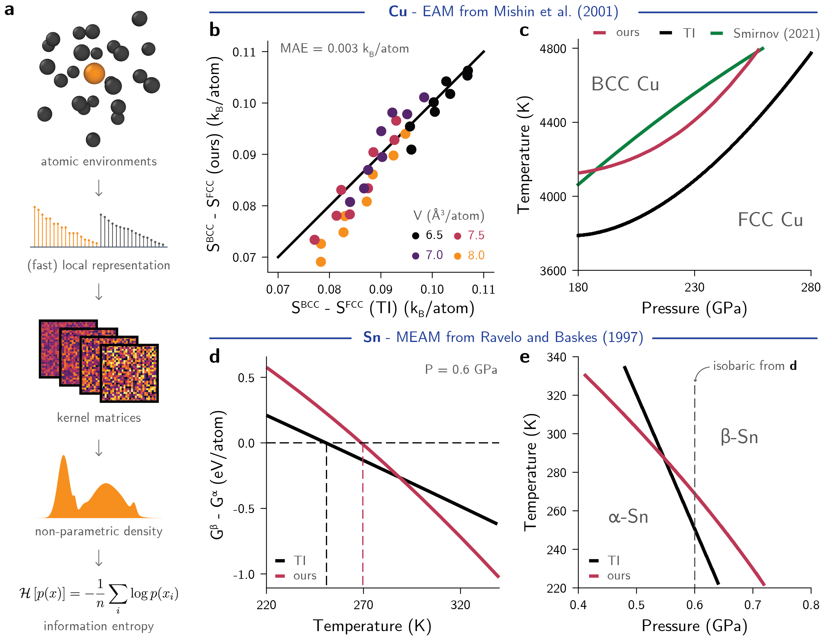
Figure 1: Information entropy is a surrogate for thermodynamic entropy differences. a, Schematic of the information-theoretical approach to obtain the information entropy of local atomic environments. A Gaussian kernel between the site-centered descriptors is used to produce a non-parametric estimate for the probability distribution (see Sec. II.1). b, Entropy differences between BCC and FCC Cu at different temperatures and densities, as obtained by thermodynamic integration (TI) and our method, are nearly identical. Higher atomic volumes are shown with brighter colors. Different points with the same color correspond to different temperatures at the same volume. c, Phase boundaries of Cu computed using our method (red) and from TI (black) using a force field are similar in shape and ranges. A reference phase boundary from the literature, computed using DFT and a quasiharmonic approximation, is shown in green.³⁷ d, Differences in Gibbs free energy between $\alpha$ and $\beta$ phases of Sn at 0.6 GPa using our method (red) and TI (black). Despite the different approaches to compute $G$, the results are consistent in values and correctly predict a phase transformation around the same temperature ranges. e, The phase boundaries between $\alpha$-Sn and $\beta$-Sn computed using our method (red) and TI (black) show good agreement across a range of pressures and temperatures.

To demonstrate that entropy differences can be computed beyond constant volume assumptions, we analyzed the phase transformation between the $\alpha$ and $\beta$ phases of tin using the modified EAM (MEAM) potential from Ravelo and Baskes.³⁸ In this transformation, the density undergoes a change of approximately 20% from $\alpha$- to $\beta$-Sn. First, we obtain the free energies with TI by mapping from the NVT to NPT space to ensure the consistency of the calculation at different values of $\lambda$ (see LABEL:sec:methods). On the other hand, our QUESTS approach allows computing entropies directly from NPT simulations for each phase. From these results, we compute the free energy differences at each (P, T) as $\Delta G=\Delta U-T\Delta S+P\Delta V$, where $U$ and $V$ are obtained from the average energies and volumes during the simulations. Figure 1d shows that the free energy differences between our method and TI at constant pressure of 0.6 GPa are in reasonable agreement. Small errors in entropy differences in our method lead to a larger derivative of the free energy curve and overestimate the transition temperature by about 10%. Across a range of pressures and temperatures, the agreement between our method and TI is shown on the phase diagram of Fig. 1e. Although differences in transition temperatures suggest that the accuracy of our method can be further improved, this quantitative agreement between descriptor distributions, information entropy, and statistical mechanics can simplify computations in first-principles thermodynamics.

Table 1: Comparison between information entropy ($\Delta\mathcal{H}$) and experimental entropies of melting ($\Delta S_{m}$), derived from experimental melting enthalpies ($\Delta H_{m}$) and temperatures ($T_{m}$) at 1 bar. The environments for solid and liquid phases were obtained from the DC3 dataset.³⁹ In this dataset, the structures correspond to: FCC Al, BCC Fe and Li, HCP Ti, and diamond Si and Ge.

Element	$\Delta H_{m}$ (kJ/mol)	$T_{m}$ (K)	$\Delta S_{m}$ ($k_{B}$)	$\Delta\mathcal{H}$ ($k_{B}$)
Al	10.7	933	1.38	1.36
Fe	13.8	1811	0.92	0.83
Ge	36.9	1211	3.67	3.15
Li	3.0	454	0.80	1.26
Si	50.2	1687	3.58	3.03
Ti	14.2	1943	0.88	1.12

As an additional example beyond solid-solid phase transitions, we computed entropies of melting of different elements obtained using our QUESTS method and the DC3 dataset.³⁹ By analyzing results from independent simulations, we verified whether our method can be generalized to obtain thermodynamic quantities solely from dataset analysis. To do that, we computed the information entropy difference between the liquid and the solid phase at the melting temperature for Al, Fe, Ge, Li, Si, and Ti in the DC3 dataset, and compared the results with their experimental melting entropies. The results are shown in Table 1. While a direct comparison between experimental and computational entropies depends on the accuracy of the interatomic potential employed in the simulation, the convergence of the entropy calculation, and many other factors, we observed that our method predicts melting entropies from the simulations that generally agree with experimental results. For Al and Fe, the information entropy of melting is quite close to the experimental values, with an error smaller than $0.1k_{B}$/atom. For Li and Ti, our method overestimates the entropy of melting by $0.46$ and $0.26k_{B}$/atom, respectively. In the cases of Ge and Si, our method correctly predicted entropies much larger than the results for the other elements, but underestimated the values compared to experimental entropies. Because these systems experience a semiconductor-to-metal transition upon melting, we hypothesized this discrepancy can be related to the electronic entropy component missing in our information entropy of the vibrational contribution only. Indeed, when density of states from DFT calculations are used to compute the electronic entropy of melting for Si and Ge, we obtain values of 0.17 and 0.11 $k_{B}$/atom, respectively. When these values are added to the QUESTS-predicted entropy, we obtain errors around $0.4k_{B}$/atom for both Si and Ge, in line with the error seen for Li and Ti. Although the values of entropy of melting can greatly vary with the choice of potential, contributions to the total entropy, and other factors, the analysis also demonstrates that the interatomic potentials used for Si and Ge^{40, 41} correctly produce a much richer phase space for their liquid phase compared to other elements. Accordingly, this approach to quantifying information entropy and recovering meaningful thermodynamic values can be extended in the future to efficiently estimate the computation of phase boundaries of many other systems while using a fraction of the computational cost of TI.

II.3 Information-theoretical description of kinetics in simulations

Beyond systems at equilibrium, free energy is also the main component of a number of kinetic transitions and out-of-equilibrium events. When analyzing these phenomena using computation, entropy cannot be quantified using TI or methods that assume equilibrium conditions, and may be ill-defined in some cases. To bypass this limitation, we use the QUESTS approach to compute the information entropy along a kinetic event by analyzing the distribution of descriptors in each frame of a trajectory. In this case, although the entropy may not correspond exactly to the thermodynamic entropy, it behaves like an order parameter for a phase transformation, where the equilibrium states have an interpretable, quantitative value for this parameter. As a model system, we simulated the nucleation of copper using the potential from Mishin et al. with an undercooling of approximately 420 K, pressure of 1 bar, and nearly 300,000 atoms in the simulation cell. The main stages observed during the trajectory included: (1) nucleation of a crystal from the melt; (2) crystal growth regime; and (3) solidified system with residual liquid and grain boundaries (Fig. 2a). The nucleation event was obtained by gradually decreasing the temperature of the molten system (Fig. 2b) over 2 ns, and verified by post-processing the results. Classification of the atomic environments using the common neighbor analysis (CNA)⁴² reveals the appearance of a dominant FCC phase in the second half of the simulation, with rapid growth for about 100 ps, and a plateau in later stages (Fig. 2c).

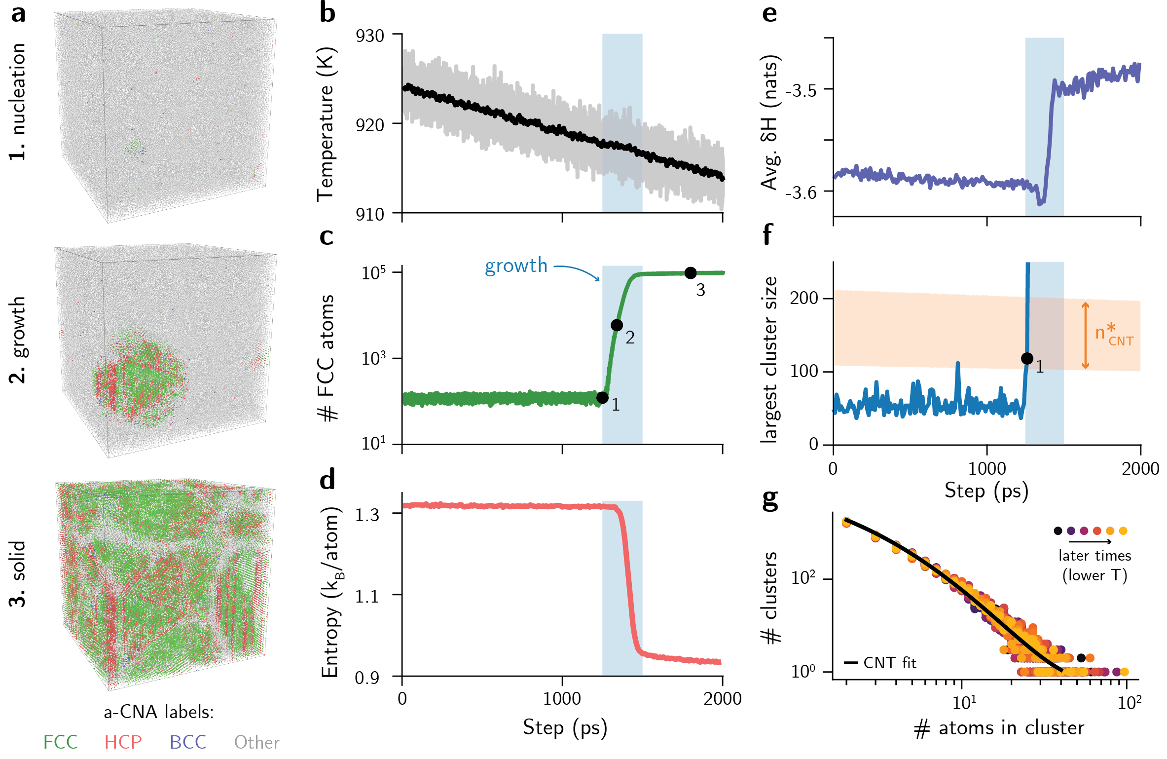
Figure 2: Information entropy is an order parameter for rare events and recovers the classical theory of nucleation. a, Visualization of the solidification trajectory during the nucleation, growth, and solid states. FCC, HCP, and BCC phases are shown with green, red, and blue colors, respectively. Non-identified phases are represented in gray. b, Average (black) and instantaneous (gray) temperature and c, number of FCC atoms derived from the MD simulation. The shaded blue area indicates the time window where crystal growth is observed. The critical nucleus is observed around 917 K. The black dots indicate the frames corresponding to nucleation, growth, and final solidified system visualized in a. d, Entropy computed for each frame using our information theoretical method. e, Average $\delta\mathcal{H}$ using the first frame (melt) as reference for the entire solidification trajectory. The drop in the average $\delta\mathcal{H}$ around 1.25 ns suggests that the phases during growth are well-represented in the melt. f, Largest cluster size in the simulation box, obtained by grouping atoms with $\delta\mathcal{H}\leq 0$. The orange lines represent the range of estimated critical nuclei sizes estimated using the experimental interfacial energy and average undercooling for each time step. g, Cluster size distribution in the melt prior to nucleation. The size distribution follows a power law similar to predictions from the CNT (fitted black line).

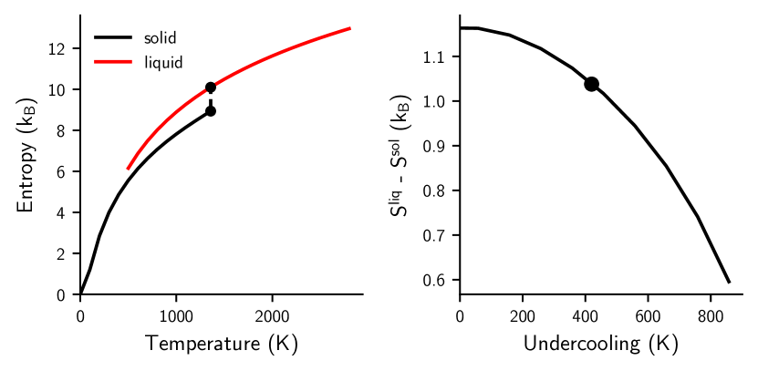
Figure S11: Absolute entropies of solid and liquid copper extracted from the NIST-JANAF tables (left), and estimated entropy change as a function of undercooling (right). The dots on the left panel indicate the experimental melting point. The black dot on the right panel corresponds to the undercooling shown in the main paper (420 K), which has an estimated entropy change of 1.038 $k_{B}$.

To quantify the information entropy along this trajectory but maintain the consistency with the thermodynamic variables at the equilibrium states, we computed the amount of information of each saved frame using our method and a fixed bandwidth of 0.057 Å^-1. This bandwidth corresponds to the one obtained for the mean of atomic volumes of solid and melt and the relation in Fig. S8. The resulting information entropy along the solidification trajectory is shown in Fig. 2d. We find an entropy change during the solidification process of approximately 0.38 $k_{B}$/atom. As a reference, the experimental entropy of fusion of copper at ambient pressure and 1357.8 K is 1.17 $k_{B}$/atom, and the entropy of fusion computed with the EAM potential is 1.09 $k_{B}$/atom.⁴³ This discrepancy between our method and the reference values can be explained by three effects: (1) the undercooling lowers the entropy difference between the liquid and solid phases (Fig. S11); (2) the end point of the simulation has not fully solidified; and (3) the final product is not a single, pure crystal. Otherwise, good qualitative and semi-quantitative agreement is obtained. To demonstrate the effects of (2) and (3), we observe in Fig. 2c that not all atoms are classified as FCC atoms. In fact, nearly 40% of the approximately 300k atoms in the simulation are classified as “other” by the adaptive CNA algorithm,⁴⁴ and 18% correspond to HCP phases crystallized as defected (mis-stacked) interfaces. The existence of these phases are also visualized in Fig. 2a by the gray areas (liquid) and red planes (HCP). As an estimate for the actual entropy change, we combine the effects of the undercooling ($\Delta S^{\mathrm{900\ K}}\approx 0.87\Delta S^{\mathrm{1358\ K}}$) and the partial solidification (factor of approximately 0.6), reaching a value of 0.57 $k_{B}$ between the liquid and crystallized phase. Indeed, if we compute the entropy difference between the melt and a pure FCC Cu structure at 915 K using our method, the resulting entropy difference is 0.60 $k_{B}$/atom. Thus, the higher diversity in atomic environments of 0.22 $k_{B}$/atom observed in the solid phase and quantified by the QUESTS method within the entropy order parameter of Figs. 2a,d must be due to defects, stacking faults, grain boundaries, and other structural features.

Beyond the thermodynamic variables, it is useful to verify whether the transient nucleation and growth can be modeled using the concept of information entropy. To analyze the configuration space accessed by the trajectory during nucleation and growth, we computed the differential entropy $\delta\mathcal{H}$ during the simulation using Eq. (6) with the first frame of the simulation used as the reference dataset for the calculation. As the first frame corresponds to the pure melt, the values of $\delta\mathcal{H}$ indicate how well represented each environment of the test frame is compared to the melt. Figure 2e shows the average values of the differential entropy $\delta\mathcal{H}$ across each frame of the simulation. Prior to nucleation, the average $\delta\mathcal{H}$ steadily decreases with the temperature, representing the decrease in phase space sampled during the simulation. At the onset of growth around 1.25 ns into the simulation trajectory, the average $\delta\mathcal{H}$ suddenly drops. Finally, as the solid phase becomes dominant, the higher values of $\delta\mathcal{H}$ show that the solid phase is less represented in the melt than the liquid phase, as expected. Nevertheless, the average differential entropy is still negative, indicating that the phase space of the solid is still present in the liquid phase. As the definition of $\delta\mathcal{H}$ is related to a functional derivative of the information entropy relative to an explored phase space (LABEL:sec:stext, Sec. .4), the decrease in $\delta\mathcal{H}$ during the growth phenomenon may be analogous to a discontinuous heat capacity from the first-order phase transition. Indeed, fluctuations in entropy are related to the heat capacity, and a discontinuity in $\delta\mathcal{H}$ during the phase transformation would explain a divergence of this value during the rare event.

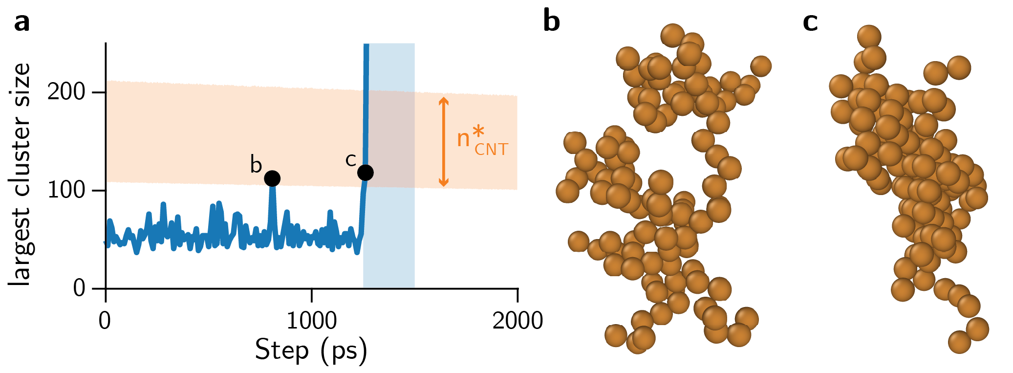
Figure S12: a, maximum cluster size throughout the solidification trajectory, as depicted in Fig. 2f of the main paper. The black dots indicate two frames when the maximum cluster size surpasses the minimum required for nucleation. The visualization of these two clusters is shown in b and c. Whereas both have approximately the same number of atoms, b is much less compact compared to c, and may be better represented by two separate clusters instead of one. This may be an artifact of the graph-theoretical approach used to identify connected atoms in the simulation cell given values of $\delta\mathcal{H}$.

This existence of solid clusters in the liquid phase is a typical assumption from the classical nucleation theory (CNT), which uses near-equilibrium assumptions to model an out-of-equilibrium event. However, quantifying their distributions directly from atomistic simulations can be challenging. Discrete classification of the solid phases, e.g., using a-CNA, typically prevents identification of the structure of the liquid phase, as very few clusters are found and classified correctly as solid-like when they are found in the melt. To verify if our information theoretical model would reproduce expected phenomena from nucleation theory, we computed the values of $\delta\mathcal{H}$ for each frame in the simulation, but this time using an MD trajectory of pure FCC copper as reference. To ensure a conservative estimate of what defines a “solid-like” cluster, the reference dataset was taken from MD simulations at a lower temperature of 400 K and pressure of 1 bar in the NPT ensemble. Then, frames of the original solidification trajectory were compared against snapshots of this low-$T$ reference MD. Instead of considering environment labels assigned by an algorithm, we propose that nuclei in the melt are formed by environments with high overlap with the phase space of the pure solid. In practice, this means that subcritical nuclei can be identified by taking environments $\mathbf{X}_{\mathrm{melt}}$ such that $\delta\mathcal{H}(\mathbf{X}_{\mathrm{melt}}|\{\mathbf{X}_{\mathrm{solid}}\})<0$, and generalizes the nucleation theory to a continuous space rather than a discrete one. Using this method, we obtained the number and size of clusters by using a graph theoretical analysis, where nodes are environments with $\delta\mathcal{H}\leq 0$, edges connect nodes at most 3 Å apart, and clusters are the sets of connected components (LABEL:sec:methods). Then, we analyzed the largest cluster size among all extracted subgraphs (Fig. 2f). With this analysis, we observed the largest cluster size is typically below 100 atoms until the nucleation event, when it reaches the value of 114 atoms. In contrast, the CNA method recovers a maximum of 170 FCC-like environments within the entire simulation box and across all pre-nucleation frames. To compare this with predictions from the CNT, we calculated the critical nucleus size given the average, time-dependent undercooling. The melting enthalpy and temperature for the EAM potential were also used to perform such estimate.⁴³ Furthermore, the solid-liquid interfacial energy was adopted from the experimental range between 0.177 and 0.221 J/m² for copper.^{45, 46, 47} This range of predictions is shown in Fig. 2f in orange. The results demonstrate that nucleation happens when the largest cluster identified by our information theoretical method falls roughly within the range of experimental critical nucleus sizes. Prior to the nucleation event, only a single other frame intersects the region of maximum cluster size. Visualization of the cluster indicates that the graph at that frame is better approximated as two nuclei rather than a single favorable critical nucleus (Fig. S12). On the other hand, the critical nucleus from point 1 in Fig. 2a,f approaches a more convex shape compared to the other outlier.

Beyond the critical nuclei, we verify that the distribution of cluster sizes in the melt can also be predicted using our approach. Figure 2g shows that, for all pre-nucleation snapshots, the cluster sizes follow approximately a power law. An analytical expression derived from the CNT (LABEL:sec:methods), when fit to the data, also perfectly matches the data distribution, with a predicted surface energy of about 0.104 J/m². While this value underestimates the experimental range of 0.177–0.221 J/m²,^{45, 46, 47} it is still remarkably close to the overall data considering the approximations of the cluster definition, surface-to-volume ratios, and other factors not accounted for in our approach. This agreement between the CNT analysis and information entropies suggest that our method can be extended to analyze other principles of nucleation and growth theories or other kinetic events, and elucidate other dynamic process in materials simulations.

II.4 Information-theoretical dataset analysis for machine learning potentials

In the previous sections, we showed how distributions of atom-centered representations connect information and thermodynamic entropies. Whereas obtaining thermodynamic entropies can be useful to analyze physically motivated phenomena from simulations, the information component of the same approach can be used to improve atomistic ML models. For example, non-global MLIPs typically predict potential energy surfaces from fixed or learned atom-centered representations. Despite the wide usage of these models, constructing optimal datasets for these potentials is still a challenge.^{48, 49, 50} Works such as the ones from Perez et al. proposed quantifying entropy as a way to build diverse atomistic datasets,^{35, 49} but their approximation to entropy in the descriptor space prevents recovering true values of information, as defined by information theory, from datasets. Within information theory, the entropy of a probability distribution has a lower bound of zero (in the case of a Dirac delta distribution) and an upper bound (in the case of a uniform distribution) that depends on the support of the distribution (see LABEL:sec:stext). Furthermore, while training models on large amounts of data can enhance the generalization power of NNIPs,^{51, 52, 53} it is still unclear whether training sets can be made more efficient while achieving similar or better results. As generating training data requires computationally-expensive ground truth calculations and large dataset sizes lead to more expensive training routines, it is important to understand how to minimize dataset sizes while maximizing their coverage in the configuration space.

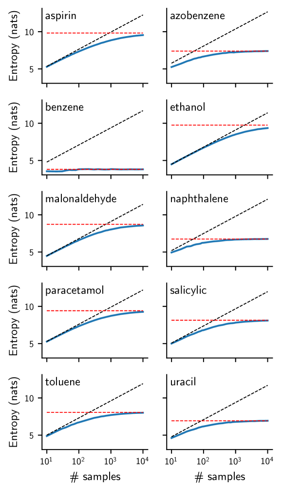
Figure S13: Entropies for all rMD17 molecules as a function of training set size. The black dashed line is the behavior of $\log n$ considering the number of environments per molecule. The red line is the asymptote for the entropy.

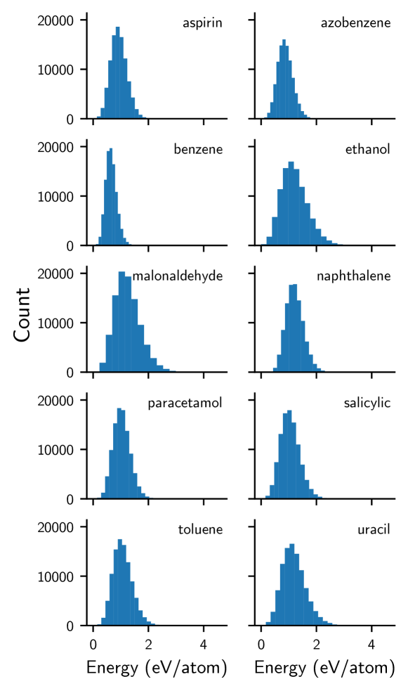
Figure S14: Distribution of energies for the original rMD17 dataset. Ethanol and malonaldehyde have larger standard deviations and longer tails towards higher energies.

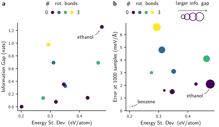
Figure S15: Correlation between the force errors from a MACE model,²⁸ the standard deviation of the distribution of energies, and the information gap for each molecule (represented with marker sizes). For the systems with zero rotatable bonds, the error is higher for wider distributions.

Borrowing from a fundamental concept in information theory, we hypothesize that the information entropy of atomistic datasets indicates the limit of their (lossless) compression, and can thus explain results from learning curves in MLIPs. The theoretical results from information theory already guarantee the compression limits that can be applied to any generic dataset,² but it is not clear whether the same effect can be observed in atomistic datasets. If true, this enables us to: (1) explain trends in learning curves in ML potentials; (2) quantify redundancy in existing datasets; and (3) evaluate the sampling efficiency of iterative dataset generation methods. As an initial test for (1), we computed the entropy $\mathcal{H}$ as a function of dataset size of different molecules in the rMD17 dataset,²² which has been widely used to evaluate the performance of different MLIPs. The bandwidth was adopted as a constant value of 0.015 Å^-1 to ensure that data points have small overlap, which represents an underestimation of the extrapolation power of MLIPs. The information entropy of six selected molecules is shown in Fig. 3a (see Fig. S13 for all molecules). At the low data regime, the total dataset entropy increases rapidly with the number of samples. On the other hand, in the high data regime, the values of $\mathcal{H}$ quickly saturate because little novelty is obtained from more data points sampled from the same MD trajectories. As expected, the saturation point depends on the molecule under analysis. Benzene, a stiff molecule with six redundant environments for both carbon and hydrogen, reaches its maximum entropy in less than 100 samples. Azobenzene, a molecule with atomic environments exhibiting two- and four-fold degenerate environments, approaches its maximum entropy value at 1000 samples. A similar behavior is seen in uracil, which has degenerate connectivity despite differences of composition. As our method does not consider composition effects, the true values of information may vary, though the diversity of vibrational motion is still captured by the descriptor distributions. The datasets of aspirin, a much more diverse molecule, are not fully converged even at 10,000 samples. As this molecule has more rotatable bonds and unique atomic environments than its counterparts, it is expected that its information content is larger, as shown by its higher entropy, and requires more samples to saturate. Ethanol is an outlier for this trend. Despite being much smaller than the other molecules, its information entropy takes a long time to reach a maximum, which is unexpected at first. To explain this result, we notice that the distribution of energies for the rMD17 dataset varies according to the molecule (Fig. S14). Molecules such as ethanol and malonaldehyde, despite small, have broader distributions compared to their counterparts, which correlates positively with higher information gaps (Fig. S15a). Thus, if we assume that energy distributions correlate with the accessible phase space on a per-system basis, then the information gap correctly captures this effect for the molecules, including ethanol, explaining this counterintuitive outlier.

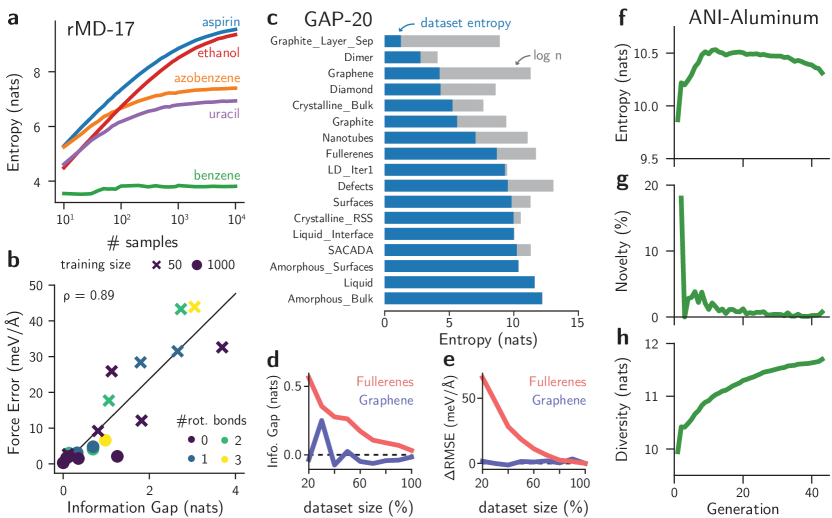
Figure 3: Information entropy measures dataset completeness, compressibility, and sample efficiency in MLIPs. a, Information entropy of selected molecules from the rMD17 dataset as a function of the dataset size. Simpler molecules exhibit lower entropy and converge faster, while more diverse molecules require more samples to converge. b, correlation between the error in predicted forces and the information gap for all molecules in the rMD17. The errors were obtained from Ref. 28 for MACE. Higher number of rotatable bonds is shown with brighter colors. A circle indicates errors when 1000 samples are used to train the models, and crosses are errors when only 50 samples are used to train the models. $\rho$ is the Pearson’s correlation coefficient. c, information entropy (blue bars) of each subset of the GAP-20 dataset. The maximum entropy is given by $\log n$ (gray bars), where $n$ is the number of atomic environments. The results are sorted by ascending dataset entropy. d, information gap obtained by compressing the “Fullerenes” and “Graphene” subsets of GAP-20 by up to 20% of their original sizes. While the information gap of “Graphene” remains close to zero, the one from “Fullerenes” monotonically increases as the dataset size decreases. e, test errors relative to the errors obtained when a MACE model is trained on the full subset of GAP-20. The results show that the “Graphene” subset can be compressed by up to 20% of its size without loss of performance, whereas this is not the case for the “Fullerenes” subset. f, information entropy for the ANI-Al dataset computed for each generation of active learning. Oversampling of certain phases leads to a total reduction of entropy. This is further supported by as demonstrated by g, showing decreasing novelty in the samples. In this approach, novelty is the fraction of environments showing $\delta\mathcal{H}>0$ when the dataset of all previous generations are taken as reference. h, Despite the reduction in entropy, the diversity of the dataset increases monotonically, showing that the phase space continues to expand, though at lower efficiency.

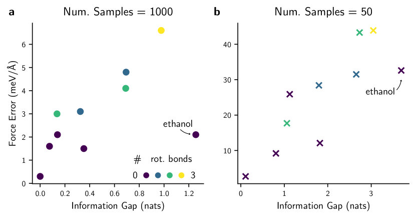
Figure S17: Correlation between the force errors from a MACE model²⁸ and the information gap for each molecule. The errors are shown separately for the model trained on two dataset sizes: a, 1000 samples and b, 50 samples. The color represents the number of rotatable bonds for each molecule. Ethanol is an outlier from the trend in a.

We hypothesize that the mismatch between the amount of information in each molecule and the constant number of samples used can partially explain the trends in testing errors across models. To validate this observation, we compared the information gap — defined as the information entropy difference between asymptotic and finite sample size values in Fig. 3a — with the testing errors reported for MACE models trained on these per-molecule dataset splits.²⁸ The correlation between the two quantities is shown in Fig. 3b, and the information gap curves are shown in Fig. S16. The information gap is a strong predictor of the error in forces, with a Pearson correlation coefficient of 0.89. Even for a constant number of samples (Fig. S17), the information gap explains major variations in force errors for the models, with the ethanol molecule being the only exception to the trend. This suggests that, in a typical MLIP model, the information gap may relate to a minimum theoretical error that can be achieved across a sampled PES, similar to the lossless compression theorem for information theory. Conversely, test errors for molecules such as benzene may be equivalent to the training error of the models, as a near-zero information gap suggests that the training set contains complete information about a given configuration space. As the benchmarks in the literature are performed at a constant number of samples, test errors vary due to differences of information content in each subset, and the information metric can be used to create trade-offs between accuracy and training set sizes.

Analogously, this notion of completeness can be useful to post-process existing datasets and quantify redundancy due to sampling and data curation. Within information theory, entropy is used to inform the development of lossless compression algorithms and encoding methods, which is closely related to our goal of dataset reduction without loss of information. To demonstrate this approach beyond the rMD17 molecular dataset, we computed the entropy of different subsets of the GAP-20 dataset.⁵⁴ The comparison between the subset entropy and the maximum possible entropy for a dataset with the same number of environments is shown in Fig. 3c. This difference between the maximum possible entropy and the subset entropy, shown with grey bars in Fig. 3c, is the opposite of the information gap. Instead of quantifying how much information is needed to reach a converged dataset, a large difference between $\log n$ and the dataset entropy often indicates oversampling in a dataset. In the field of MLIPs, test errors are typically used to quantify saturation of a dataset.⁵⁴ However, our information theoretical analysis provides absolute bounds to the entropy and quantifies the completeness of the dataset without training any model. For example, the difference between the actual information contained in the “Graphene” subset of GAP-20 and the absolute limit given by $\log n$ shows that this subset has large redundancy compared to the “Fullerenes” subset, where the difference between the maximum and actual entropy is smaller. The bounds also illustrate how different datasets can exhibit larger diversity. For example, structures labeled under the “Liquid” and “Amorphous$\_$Bulk” categories are maximally diverse, with environments mostly distinct with the bandwidth used to compute the KDE (0.015 Å^-1, see LABEL:sec:methods). This may be a consequence of both the larger accessible phase space by these amorphous and liquid structures and the original farthest point sampling approach used when constructing the dataset.⁵⁴

To illustrate the relationship between information entropy and dataset compression, we computed the entropy curves of different subsets of the GAP-20 dataset. Then, we trained a NNIP based on the MACE architecture²⁸ on (judicious) fractions of the subsets, computing test errors as a function of training set size and, thus, entropy. Fig. 3d exemplifies this relationship for the labels “Graphene” and “Fullerenes” of GAP-20, which exhibit large (Graphene) and small (Fullerenes) levels of redundancy (Fig. 3c). In the former, datasets as small as 20% of the original one still exhibit entropies around 4.25 nats, similar to the full one. Accordingly, their test errors remain constant across all dataset sizes (Fig. 3e), with a value of 0.96 $\pm$ 1.37 meV/Å  for force errors relative to model trained on the full training set. Despite fluctuations in total entropy caused by the random sampling approach — which depend on unit cell sizes and ordering of structures in the dataset, and become more sensitive at the low-data regime — these results show that our model-free analysis of dataset entropy correctly informed the redundancy of the dataset. On the other hand, the dataset labeled as “Fullerenes” is less redundant, and subset entropies monotonically decrease as the training set size goes down. As expected, the test errors also increase with smaller training set sizes, reproducing known patterns in learning curves of MLIPs (Fig. 3e). Although this example considers only a random sample of data points when “compressing” a dataset, different algorithms can be used in future work to evaluate optimal subsets with maximum entropy for compression of training sets for MLIPs⁵⁵ or also evaluation of extrapolation and completeness in fast data generation approaches.⁵⁶

Finally, to exemplify how information theory can be useful to evaluate active learning (AL) strategies in MLIP-driven atomistic simulations, we analyze dataset metrics of the ANI-Al dataset,⁵⁷ which constructed a dataset for aluminum by starting from random structures and performing over 40 generations of sampling and retraining with NNIP-driven MD simulations. Figure 3f shows how the entropy varies as new configurations are sampled by the AL. In the initial stages of the active learning, the entropy of the dataset quickly increases, then peaks around generation 12, before subsequently decreasing. To explain this effect, we observe that the increase in diversity of this dataset⁵⁷ comes at the cost of oversampling certain regions of the configuration space. In fact, fewer than 5% of the environments sampled after the third round of AL are novel according to our information-theoretical criterion (Fig. 3g). This suggests that although MD simulations provide a physically meaningful way to sample new configurations, most sampled configurations may be already contained in the original training sets. This may be especially true for large periodic cells where a handful of unknown environments (i.e., $\delta\mathcal{H}>0$) may not be easily separated from the numerous known (or similar-to-known) environments ($\delta\mathcal{H}\leq 0$) that may surround them. To verify that the total coverage of the configuration space still increases, we propose an additional metric of dataset diversity $D$,

$$D\left(\{\mathbf{X}\}\right)=\log\left[\sum_{i=1}^{n}e^{\delta\mathcal{H}(\mathbf{X}_{i})}\right],$$ (8)

that reweights each data point’s contribution to the information entropy based on how well-sampled its region of the configuration space is (LABEL:sec:stext, Section .7). Indeed, Figure 3h shows how the dataset diversity continues to grow even when the entropy decreases. This approach of measuring dataset diversity is related to the concept of “efficiency” in information theory² and may be used to propose new ways to sample atomistic configurations or automatically create datasets for MLIPs in the future.

II.5 Model-free uncertainty quantification for machine learning potentials

When information theory is used to analyze a single dataset, as in the previous section, environments are compared against other environments in the same dataset. However, reference datasets $\{\mathbf{X}\}$ may not contain the tested sample $\mathbf{Y}$, often leading to $\delta\mathcal{H}(\mathbf{Y}|\{\mathbf{X}\})>0$. As such, we propose that differential entropies can be used as a model-free uncertainty estimator for a given dataset. Whereas uncertainty quantification (UQ) methods for MLIPs usually rely on models^{58, 59} — i.e., prediction uncertainties are associated to variances in model predictions — we propose instead that UQ can be performed based on the data alone. This approach is similar to Gaussian process regression methods,^{19, 60, 61} which compute an uncertainty by inverting a covariance matrix computed for training points, or parametric models on a latent space.⁶² Differently from other approaches, however, our method performs a fast non-parametric estimate directly on the atomistic data space, thus bypassing the need for a model. While this approach can be expensive for large datasets, it is easily parallelizable, is backed by theoretical results, and is guaranteed to provide a robust uncertainty estimate, as it does not rely on the randomness associated with model training or inference.

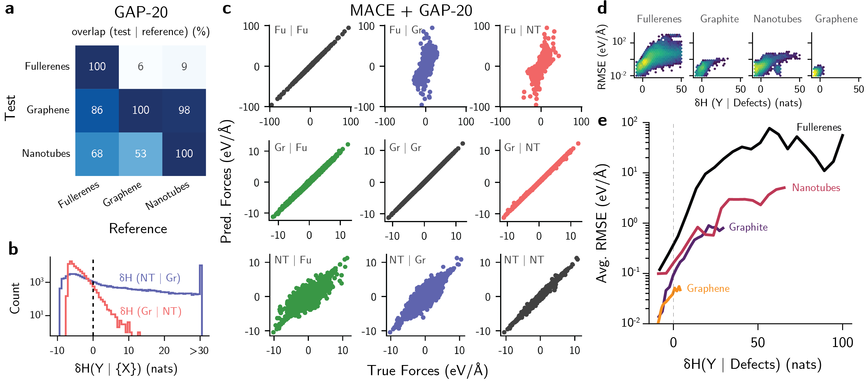
Figure 4: Information entropy quantifies overlaps between datasets and is a model-free UQ method. a, Overlap between test and reference sets for the GAP-20 carbon dataset. Only a subset of the data is shown for clarity (see Fig. S18 for complete matrix). b, Histogram of differential entropies for the nanotubes (NT) and graphene (Gr) subsets of GAP-20. The small number of positive $\delta\mathcal{H}$ (GR | NT) values shows that the “Graphene” split is nearly contained in the “Nanotubes” split, but not the other way around. c, Test errors of a MACE model trained either on the fullerenes (Fu), graphene (Gr), or nanotubes (NT) subset of the GAP-20 dataset. Parity plots exhibiting higher errors are those with lower overlaps between train and test sets shown in a. d, Correlation between RMSE and $\delta\mathcal{H}$ for a MACE model trained on the Defects subset of GAP-20. The values of $\delta\mathcal{H}$ are computed using the training and validation set of the model as reference. The $\delta\mathcal{H}$ was truncated to 50 nats for clarity. Brighter colors indicate higher density of points. e, The average RMSE increases with higher $\delta\mathcal{H}$. The $\delta\mathcal{H}$ was truncated to 100 nats for clarity.

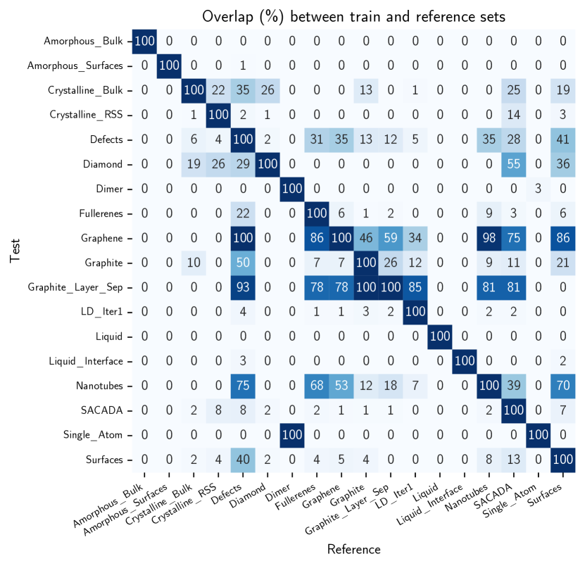
Figure S18: Overlap between test and reference sets for the GAP-20 carbon dataset.

To exemplify how information theory can be used for UQ in MLIPs, we computed the values of $\delta\mathcal{H}$ for different subsets of the GAP-20 dataset discussed in the previous section. Then, we compute the overlap between one subset given another reference set of configurations. Figure 4a exemplifies the values of these overlaps for the “Fullerenes” (Fu), “Graphene” (Gr), and “Nanotubes” (NT) subsets of the dataset (see Fig. S18 for complete results). The results show that environments in the “Graphene” split are mostly contained in the other two subsets, with a minimum overlap of 86% between “Graphene” and “Fullerenes”. On the other hand, “Fullerenes” contains a sizeable portion of “Nanotubes”, with an overlap of 68%, but not the other way around. Similarly, “Nanotubes” contains almost all environments of the “Graphene” dataset, but “Graphene” contains only 53% of the environments in “Nanotubes,” as also illustrated in Fig. 4b. This analysis also allows us to identify how each subset is constructed without having to label the structures beforehand. For example, Fig. S18 shows that the “Graphene” subset is also contained by the “Defects” and “Surfaces” datasets, but not fully covered by the “Graphite” dataset. The subsets labeled as amorphous or liquid do not overlap with any of the others, even though their phase space could have been similar depending on their construction method. Finally, large subsets such as “Defects” and “SACADA” contain several parts of the other subsets, largely due to the way they were created. While there were labels available for the GAP-20 dataset, this overlap analysis can be used to compare pairs of datasets in general, regardless of available labeling.

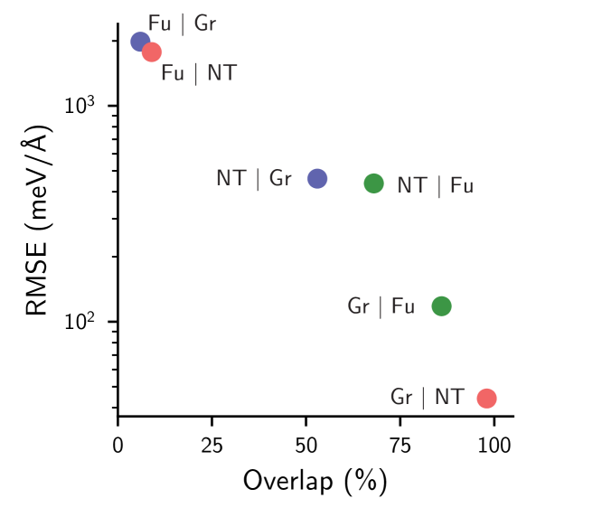
Figure S19: The RMSE of forces for MACE models trained on different subsets of the GAP-20 dataset and the overlap between train and test sets follows a power law, with higher overlap leading to lower errors.

To verify whether overlap between training and testing sets is useful as a predictor of uncertainty and error metrics, we trained MACE models to one of the “Graphene”, “Fullerenes”, and “Nanotubes” subsets of GAP-20, then tested the models on the three splits. Figure 4c shows the test errors obtained from such training-testing splits. When models are tested on the “Graphene” subset, all of them perform near perfect predictions, as expected by the high overlap between the “Graphene” subset and the others. Models tested on the “Nanotubes” subset exhibit higher errors, with the MACE model trained on “Fullerenes” showcasing a slightly better result compared to the one trained on “Graphene.” Finally, models tested on “Fullerenes” but trained on the other two subsets perform poorly and exhibit large errors in forces. These results reproduce exactly the trends in Fig. 4a, and the errors follow a power law for distinct train/test sets with clear anti-correlation between the error and overlap (Fig. S19).

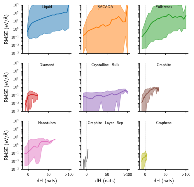
Figure S20: RMSE of forces for MACE models trained on the “Defects” GAP-20 dataset and tested on other subsets. The test splits are sorted by increasing overlap with the training sets. The shaded area represents the range of the error distribution in each window of $\delta\mathcal{H}$. For clarity, small errors are truncated to be equal to 1 meV/Å, and the plot is truncated at a maximum error of 1000 eV/Å. Because some data points in the “Liquid” or “SACADA” subsets are infinitely far away from the “Defects” training set, their values of $\delta\mathcal{H}$ are also infinite. To avoid issues with the visualization, we clipped the values of $\delta\mathcal{H}$ at 100 for all sets.

To further this observation, we trained a MACE model on the “Defects” split of the GAP-20 dataset. Then, four other splits with increasing overlaps with “Defects” were selected as test sets: “Fullerenes” (22% overlap), “Graphite” (50%), “Nanotubes” (75%), and “Graphene” (100%) (Fig. S18). Force errors were then evaluated for this model and correlated with the values of $\delta\mathcal{H}$, as shown in Fig. 4d. For environments where $\delta\mathcal{H}>0$, the RMSE is often above 0.1 eV/Å. On the other hand, when $\delta\mathcal{H}\leq 0$, errors typically stay below 0.3 eV/Å. To demonstrate that higher values of $\delta\mathcal{H}$ usually lead to higher errors beyond the correlation plots, we computed the average RMSE for each window of $\delta\mathcal{H}$. Figure 4e shows that average errors continue to increase as the values of $\delta\mathcal{H}$ also increases, showing that points with larger distances to the training set tend to exhibit larger extrapolation errors. On the other hand, points slightly outside of the known domain, thus with positive but near zero $\delta\mathcal{H}$, often show average errors comparable to the ones in the training set. Interestingly, Fig. 4e also shows that force errors continue to decrease as $\delta\mathcal{H}$ becomes more negative. This correlates with the idea that unbalanced datasets bias the training process and end up minimizing the loss for data points with higher weight (i.e., with more negative $\delta\mathcal{H}$). The same observation is valid for the maximum error within each range of $\delta\mathcal{H}$ (Fig. S20), illustrating how the differential entropy does not exhibit false negatives for the dataset and model under study, i.e., negative entropy values necessarily lead to small errors provided that errors are small everywhere in the training set. Furthermore, because the uncertainty threshold $\delta\mathcal{H}>0$ as extrapolation metric is guaranteed by the theory (LABEL:sec:stext, Section .4), our UQ metric detects points outside of the training domain without the need for additional calibration or fitting empirical parameters. Thus, our information theoretical approach provides a robust, model-free alternative to quantifying errors in MLIPs and can be used beyond NN models.

II.6 Information-based detection of outliers in large-scale simulations

To further illustrate how our information theoretical method can be used for outlier detection in large-scale ML-driven simulations, we produced an MD trajectory of (dynamically strained) tantalum using a supercell containing approximately 32.5 million atoms and the SNAP potential²¹ (see LABEL:sec:methods). In these large models, obtaining uncertainty estimates of energy/force predictions can be challenging even at the postprocessing stage, especially if it requires re-evaluating predictions with several models, such as with an ensemble approach. Furthermore, uncertainty thresholds may not be well-defined for models such as SNAP, where the choice of weights, training sets, and hyperparameters can lead to substantial variations of model performance.⁴⁹ Finally, ML-driven simulations of periodic systems may fail in completely different ways compared to simpler molecular systems,^{30, 31} where bond lengths and angles are often sufficient to detect an extrapolation behavior.

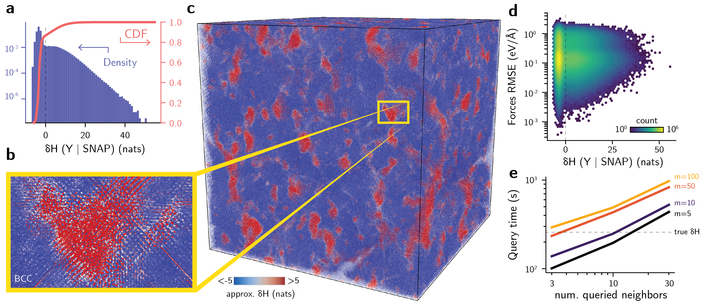
Figure 5: Differential entropies detect outliers due to extrapolation in large-scale simulations. a, Distribution (blue) and cumulative density function (CDF, red) of estimated $\delta\mathcal{H}$ values. 87% of the atoms exhibit $\delta\mathcal{H}<0$ nats and thus are reasonably close to the training set. b, Visualization of a 32.5M atom snapshot of BCC Ta simulated with SNAP. Colors represent the values of the estimated $\delta\mathcal{H}$, with blue atoms indicating environments reasonably within the training set ($\delta\mathcal{H}<0$) and red atoms indicating environments outside of the training set ($\delta\mathcal{H}>0$). Values of $\delta\mathcal{H}$ were truncated to the range $[-5,5]$ to facilitate the visualization of divergent colors. c, Example of high-uncertainty region encountered during the simulation. The formation of a disordered, non-BCC phase (red) in the simulation leads to unphysical behavior in the trajectory. d, The unphysical behavior cannot be identified only by errors in forces. Even outside of its known domain, the SNAP model exhibits errors within the range of systems within the training set. The number of environments in each region is shown by the color scale, with brighter colors indicating exponentially denser regions of the error-$\delta\mathcal{H}$ space. e, Computational performance of the approximate nearest neighbors search. At the low-resource side ($N=3$ queried neighbors per environment, index constructed with $m=5$ neighbors), the values of $\delta\mathcal{H}$ for all 32.5M atoms are evaluated in about 100 seconds when performed in a single node with 56 threads. For the SNAP dataset, the true $\delta\mathcal{H}$ for all environments is computed in about 255 s (wall-time) with the same hardware and parallelization settings.

Using the true $\delta\mathcal{H}$ for the 32.5M atom system, we analyzed a snapshot of the tantalum MD trajectory with our information theoretical method to identify possible anomalies due to extrapolation during the simulation. Figure 5a shows that about 13% of the environments exhibit $\delta\mathcal{H}>0$, some of which are as large as $\delta\mathcal{H}=55.8$ nats, showing that a substantial number of environments are outside of the training domain of SNAP. Figures 5b,c illustrates these results at the atomistic model, with colors representing the values of $\delta\mathcal{H}$ computed with respect to the training set of SNAP. Despite starting with a monocrystalline BCC structure of tantalum (in blue colors, often within the SNAP training set), the simulation proceeded to form amorphous-like phases (Fig. 5b) that are unexpected in such trajectories. Although the model prevents obvious unphysical configurations such as overlapping atoms, distinguishing between model failures and new physical phenomena in these simulations is mostly unclear without our information theoretical approach. To illustrate this challenge, we computed the ground truth forces for the atomistic system from an interatomic potential, and analyzed the errors of the predictions (Fig. 5d). The results show that the SNAP model under investigation does not exhibit high extrapolation errors, as the forces RMSE are within the same range of errors of environments having $\delta\mathcal{H}<0$. Instead, the formation of the amorphous phase can be due to lower predicted energies compared to the true energies, which can be more challenging to compare given the global nature of this quantity. Therefore, even having access to the ground truth potential would not allow the classification of a trajectory as failed within these constraints, and instead would rely on human inspection. On the other hand, the differential entropy detects these outliers without the need for a calibrated threshold, providing a conservative estimate for understanding model extrapolation in a completely model-free approach.

At larger scales, one drawback of computing entropy values is the necessity of computing kernel matrices between each test point and the entire training set. As the number of test points $n_{Y}$ and training examples $n_{X}$ grow, the cost of computing such matrices increases with $\mathcal{O}(n_{X}n_{Y})$. To verify if this is a problem in a large atomistic model, we approximate the values of $\delta\mathcal{H}$ by truncating the summation in Eq. (6) and using an approximate nearest neighbors approach (see LABEL:sec:stext, Section .5), which decreases the complexity to $\mathcal{O}(n_{Y}N\log n_{X})$, with $N$ the number of neighbors in the descriptor space. As computing $\delta\mathcal{H}$ for each point $\mathbf{Y}$ is an embarrassingly parallel task, the search can be distributed over different processes or threads to expedite the computation of this differential entropy. Figure 5e shows the total query times for the 32.5M environments of tantalum relative to the SNAP training set (4224 environments) as a function of approximate nearest neighbors parameters and parallelized over 56 threads. As the index is constructed to increase the accuracy of the approach (higher values of $m$, see LABEL:sec:methods), larger query times are obtained, with the slowest time obtained when an index with $m=100$ is created and $k=30$ neighbors are queried for each of the 32.5M test environments. In that case, the computation of $\delta\mathcal{H}$ used a wall time of 1000 seconds when parallelized on 56 threads on 56 Intel Xeon CLX-8276L CPUs from the Ruby supercomputer. On the other hand, the fastest set of parameters ($m=5$, $k=3$, 56 threads) spent 100 seconds in the same hardware. As a reference, computing the exact $\delta\mathcal{H}$ values for the 32.5M atom system with respect to the SNAP dataset (4224 environments) takes a walltime of about 255 seconds using the same hardware and parallelization settings. While the approximate $\delta\mathcal{H}$ has better scaling for larger reference datasets and is not critical for the SNAP dataset, performing the nearest neighbor search adds additional time constants compared to the brute-force exact calculation of the true $\delta\mathcal{H}$. While the timings can further be improved with additional parallelization, code optimization, or use of GPU architectures, our results already demonstrate that the computation of the differential entropy, either in approximate or complete way, is accessible even for systems with a large number of environments.

III Discussion

Our results show how a unified information theoretical approach can be used in a range of problems in atomistic modeling. By computing distributions of atom-centered representations from simulations, we obtained quantitative agreement between information and thermodynamic entropies. This allowed us to predict phase boundaries, free energy curves, and transition entropies at low costs compared to thermodynamic integration. These surprising results may suggest that these descriptor distributions may approximate the Boltzmann distribution sampled during the MD simulations. Because the feature space of several atom-centered representations are not injective,⁶³ this property depends on the choice of descriptor. Future work can lead to other fixed or learned representations that can be computed at scale and better approximate the Boltzmann distributions, therefore enabling the computation of higher-accuracy entropies compared to the current study.

In addition to entropy at equilibrium, our method enabled proposing entropy as an order parameter along kinetically driven events such as nucleation and growth. The results paralleled experimental entropies of transition for the given undercooling and quantified the information entropy gain relative to defect formation, partial solidification, and more. Furthermore, using the notion of overlap in phase space, we showed how information theory can recover results from classical nucleation theory and identify nuclei with sizes in agreement with its postulates. Future investigations can refine the approximations used in the calculations, such as the CNT assumption of spherical clusters, constant surface energies, and so on. As determining entropy in out-of-equilibrium conditions can be challenging, our approach may open a path to understand free energies in rare events and other pathways, and rationalize different nucleation, growth, and phase transformation phenomena from atomistic simulations.

Beyond atomistic properties, our information-based analysis of datasets and uncertainty explains multiple results within learned interatomic potentials. In particular, we showed how information and diversity content in a dataset can be quantified, explaining error trends in MLIPs, rationalizing dataset compression, predicting extrapolation errors, and detecting failed simulation trajectories. Furthermore, because information entropy provides a quantitative estimation of “surprise” of a random variable, we proposed its use as a robust UQ metric for ML-driven atomistic simulations and showed it can be computed even for large atomistic systems. As this strategy does not depend on models, it can be adapted to any MLIP to provide general uncertainty metrics and may be a universal UQ method for atomistic simulations.

In future work, several improvements can help generalize the method beyond simpler simulations. For example, the approach does not take into account composition, as the representation does not account for element type. For simple molecular systems, bonding patterns (e.g., valence rules) sometimes map distributions of atomic environments to different parts of the information entropy space due to the construction of the $k$-nearest neighbors descriptor based on interatomic distances. However, for inorganic crystals, this approximation may not be valid, and may have to be incorporated into the approach to account for true configurational entropies, as seen in alloys. Moreover, although our model succeeded in predicting relative configurational entropy differences, computation of true entropy values requires incorporating effects of velocity (i.e., complete vibrational entropy), electronic, magnetic, and other components to the final results, all of which influence the phase transformations of materials. Finally, whereas the current computational implementation is sufficient for the analysis of tens of millions of environments, improvements in parallelization and hardware utilization can allow the approach to scale beyond being a post-processing tool and towards a real-time UQ for MD. Fast computation of distances using GPUs, multi-node parallelization, or better approximate nearest neighbors computation can be implemented in future versions of the code, allowing greater scaling in computing kernel density estimates and their resulting entropies. Nevertheless, the quadratic scaling of true entropy computation may be necessary for a rigorous definition of thermodynamic entropy in arbitrary datasets.

IV Conclusions

In this work, we proposed an unified view for atomistic simulations based on information theory. By performing a kernel density estimation over distributions of atom-centered features, we obtained values of information entropy that: (1) predict thermodynamic entropy in equilibrium, and extend it to out-of-equilibrium conditions as an order parameter; (2) recover classical theories of nucleation for simulations containing rare events; (3) rationalize trends in testing errors for machine learning potentials, relating model performance to information quantities; (4) proposes a compression approach for atomistic datasets based on information theory; and (5) provides a model-free uncertainty quantification approach for atomistic ML. These contributions are demonstrated with numerous examples, such as phase boundaries obtained from thermodynamic integration methods, a solidification trajectory, known benchmarks from the MLIP literature, and a simulation of a system containing about 32.5M atoms. As increasingly accurate and scalable ML models are proposed for atomistic simulations, this work proposes a rigorous way to optimize their training process, automate evaluation of thermodynamic and kinetic properties, and assess the performance of the results. Additional developments in atomistic information theory can continue to translate developments in machine learning and statistical thermodynamics into faster and more accurate materials modeling.

Methods

Information entropy and QUESTS method

Representation: the representation of atomic environments was computed as described in Section II.1 of the main text and Section .1 of the LABEL:sec:stext. Throughout this work, a number of $k=32$ neighbors was used to represent the atomic environment, with a cutoff of 5 Å. To accelerate the calculation of the representation, the code that computes the descriptors was optimized using Numba⁶⁴ (v 0.57.1) and its just-in-time compiler. For periodic systems, the feature vectors were created by adapting the stencil method for computing neighbor lists and parallelizing the creation of features across bins.

Information entropy: the information entropy of descriptor distributions was computed as described in Section II.1 of the main text and Section .2 of the LABEL:sec:stext. Throughout this work, the natural logarithm was used for the entropy computation, which scales the information to natural units (nats). The scaling of bandwidth (Section .6 of the LABEL:sec:stext) with respect to the volume calibrates the metric space to reproduce the values of $k_{B}$. However, when not specified, we adopt a bandwidth of 0.015 Å^-1. This leads to final entropy values with unscaled values compared to the Boltzmann constant $k_{B}$, but still respecting the properties of the information entropy (Section .2 of the SI). In this case, we show the units as nats instead of $k_{B}$. The procedure is similar for the computation of the differential entropy $\delta\mathcal{H}$, and the units adopted are the same.

Entropies of melting: to obtain the results shown in Table 1, we computed the average volume of each system using the same number of frames for solid and liquid phases. This enables us to estimate entropies without considering significant density changes upon melting, which could cause bandwidth values to change and lead to fluctuations in the entropy computation.

Entropy asymptotes: the asymptotic behavior of entropies in the learning curves of Fig. 3a and S13 was obtained by fitting a function of the form

$$f(N)=a-b\exp\left[-c(\log N)^{2}\right],$$ (9)

with $a,b,c$ parameters obtained from the entropy curve as a function of training set size $N$. The first and last three points were discarded during the fitting process. The fit was performed using a non-linear least squares method implemented in SciPy⁶⁵ (v. 1.11.1). This functional form was found to closely approximate the curves shown in Fig. 3a and S13.

Molecular dynamics simulations

All MD simulations were performed using the Large-scale Atomic/Molecular Massively Parallel Simulator (LAMMPS) software⁶⁶ (v. 2/Aug./2023). All simulations were performed using a 1 fs time step, except when stated otherwise.

Thermodynamic Integration: free energies of solids were computed by assuming a potential energy $U_{\lambda}$ that couples a reference system with potential energy $U_{\mathrm{ref}}$ and the interacting one $U_{\mathrm{IS}}$ such that

$$U_{\lambda}=\lambda^{2}U_{\mathrm{IS}}+(1-\lambda^{2})U_{\mathrm{ref}},$$

where the quadratic term $\lambda^{2}$ reduces the impact of sampling the space of $(N,V,T,\lambda)$ with a uniform grid in $\lambda$, and thus creates a denser sampling around $\lambda=0$ or $\lambda=1$ which mitigates numerical integration errors. The Helmholtz free energy $F$ of the interacting system is obtained first taking the derivative of the free energy of the system corresponding to $U_{\lambda}$ with respect to $\lambda$,

$$\left(\frac{dF_{\lambda}}{d\lambda}\right)_{N,V,T}=\left\langle\frac{\partial U_{\lambda}}{\partial\lambda}\right\rangle_{\lambda},$$

where $U$ is the energy of the system. Integrating the expression above in $\lambda$, we obtain

$$F_{\mathrm{IS}}=F_{\mathrm{ref}}+\int_{0}^{1}2\lambda\left\langle U_{\mathrm{IS}}-U_{\mathrm{ref}}\right\rangle_{\lambda}d\lambda,$$

where $F_{\mathrm{ref}}$ is known for any given temperature and volume. We adopted the Einstein crystal as the reference, and modified the fix ti/spring⁶⁷ in LAMMPS to obtain energies for each $(V,T,\lambda)$ without using a switching function. Using this, we performed different simulations for each point of the grid, thus ensuring stricter convergence of the average energy differences $U_{\mathrm{IS}}-U_{\mathrm{ref}}$ for each $\lambda$. We used a uniform grid with a spacing of 0.02 for $\lambda$, leading to 51 data points for each phase and $(V,T)$. Numerical integration was performed using the function from the QUADPACK library⁶⁸ interfaced by SciPy⁶⁵ (v. 1.11.1).

Entropy from TI: given the free energy computed using the TI method, the entropy by taking the derivative of the Helmholtz free energy with respect to the temperature,

$$S=-\left(\frac{\partial F}{\partial T}\right)_{N,V}.$$

As the free energy is not computed for an infinitely dense grid of $(V,T)$ values, numerical derivatives can lead to inaccurate values of entropy. To mitigate this problem, we fit a quadratic 2D polynomial to the free energies as a function of the independent variables $(V,T)$. The fit is performed using the Lasso method ($L_{1}$ regularization) for all polynomial features up to degree 2 using the scikit-learn⁶⁹ (v. 1.3.0) library, with $\alpha=10^{-4}$ and a maximum of $10^{6}$ iterations. Then, with the interpolated values of free energy, we obtain the entropy by taking the numerical derivatives of $F$ with a fine grid of temperatures at each value of volume.

Phase diagrams from TI: given the convenience of using the NVT ensemble when performing thermodynamic integration calculations, we constructed P-T phase diagrams by first obtaining free energies in the $(N,V,T)$ space. Then, using the value of average pressure for each volume, we map each point $(P,T)$ into a volume $V$, and the resulting $(V,T)$ into a free energy $F$. With these variables, we compute the Gibbs free energy as $G(P,T)=F(V(P,T),T)+P\times V(P,T)$. The functions $(V,T)\rightarrow F$ and $(P,T)\rightarrow V$ are performed as described before, thus using a two-dimensional polynomial regressor with degree 2 and $L_{1}$ regularization. We observed that direct mappings $(P,T)\rightarrow F$ led to numerical inconsistencies that drastically affected the outcomes of the phase diagram, especially given the small entropy differences between the phases. On the other hand, the step-wise mapping was found to be more numerically stable.

FCC-BCC Cu phase transition at high pressure: the phase boundary between the FCC and BCC phases of copper was simulated using the EAM potential from Mishin et al.³⁶ The phases were simulated at four volumes: 6.5, 7.0, 7.5, and 8.0 ų/atom, which correspond to the range of high pressures shown in Fig. 1b. All calculations were performed with $20\times 20\times 20$ supercells, leading to an FCC cell with 32,000 atoms and a BCC cell with 16,000 atoms. Simulations were performed at 9 temperatures between 3000 and 5000 K separated by 250 K, and 51 values of $\lambda$. The MD simulation was performed at the NVT ensemble with the Langevin thermostat implemented in LAMMPS⁷⁰ and a damping constant of 0.5 ps. The simulation was equilibrated for 100 ps before a 1 ns-long production run. During the production run, the pressure, energy, and the coupled energy $U_{\mathrm{IC}}-U_{\mathrm{ref}}$ were averaged for every time step, and later printed for post-processing in the TI approach. A spring constant of 34.148 eV/Ų was used to attach the Cu atoms to their ideal lattice sites, thus modeling the Einstein crystal.

Entropy calculations using our QUESTS method were performed in the NVT ensemble using the same temperatures and volumes as the TI method. Simulations used the same cell sizes as the TI, but had 100 ps-long production runs. Snapshots were saved every 2.5 ps. Entropy values were obtained by randomly sampling 200,000 environments of the saved trajectory with a variable bandwidth determined by their volume.

$\alpha-$ to $\beta-$Sn phase transition: the phase boundary between the $\alpha$ and $\beta$ phases of tin was simulated using the MEAM potential from Ravelo and Baskes³⁸. The equilibrium lattice parameters for these structures were found to be $a_{\alpha}=6.483$ Å, $a_{\beta}=5.830$ Å, and $c_{\beta}=3.183$ Å. All calculations were performed with a $12\times 12\times 12$ supercell for $\alpha$ and $12\times 12\times 24$ for $\beta$, leading to a cell with 13,824 atoms each. For the TI, simulations were performed at three different volumes, corresponding to 98%, 100%, and 102% of the equilibrium volumes of each phase, 7 temperature values between 200 and 350 K spaced by 25 K, and 51 values of $\lambda$. The MD simulation was performed at the NVT ensemble with the Langevin thermostat implemented in LAMMPS⁷⁰ and a damping constant of 0.5 ps. The simulation was equilibrated for 40 ps before a 500 ps-long production run. During the production run, the pressure, energy, and the coupled energy $U_{\mathrm{IC}}-U_{\mathrm{ref}}$ was averaged for every time step, and later printed for post-processing in the TI approach. A spring constant of 2.0 eV/Ų was used to attach the Sn atoms to their ideal lattice sites, thus obtaining an ideal Einstein crystal as reference system.

Entropy calculations using our QUESTS method were performed in the NPT ensemble at 1 bar and same temperatures as the TI method. Simulations used the same cell sizes as the TI, but had 200 ps-long production runs, with snapshots saved every 10 ps. Entropy values were obtained by randomly sampling 100,000 environments of the saved trajectory with a constant bandwidth of 0.038 Å^-1, which corresponds to the bandwidth for the average of the volumes between the $\alpha$ and $\beta$ phases (Fig. S8).

Cu solidification: the solidification trajectory of copper was simulated using the EAM potential from Mishin et al.³⁶ A $42\times 42\times 42$ supercell of FCC copper (296,352 atoms) was simulated above the melting point to produce the structure of the liquid, then cooled to 924 K. Starting at the temperature of 924 K, the system was cooled to 914 K over the course of a 2 ns-long simulation in the NPT ensemble with the Nosé-Hoover thermostat and barostat^{71, 72} implemented in LAMMPS. Damping parameters for the temperature and pressure were set to 0.1 and 3.0 ps, respectively, a 2 fs time step was used for the integrator, and constant pressure of 1 bar. Over the trajectory, the number of FCC atoms was computed using the common neighbor analysis (CNA) implemented in LAMMPS.⁴²

Large-scale Ta simulation: The atomistic configuration with “amorphous-like” substructures (Fig. 5) used in benchmarking performance of our information-based detection of structural anomalies resulted from a large-scale MD simulation of crystal plasticity in body-centered-cubic metal Ta. The simulation was performed using a SNAP potential fitted to the dataset of the original SNAP potential.²¹ However, rather than using the DFT ground-truth reference values of energies, forces and stress in the original fitting dataset, all the same quantities were re-computed using an inexpensive interatomic potential of the embedded-atom-method (EAM) type. Given that both SNAP and EAM simulations can be performed at scales large enough to perform simulations of metal plasticity of the kind described in Zepeda-Ruiz et al.,⁷³ the intention was to observe if a SNAP potential fitted to such a proxy training dataset could reproduce plastic strength predicted by the proxy potential itself. The SNAP simulation considerably diverged from the proxy EAM simulation both in predicted plasticity behavior and in producing the “amorphous-like” regions that never appeared in the proxy EAM simulation.

Machine learning potential

MACE architecture: the ML force fields for GAP-20 in this work were trained using the MACE architecture.²⁸ We used the MACE codebase available at https://github.com/ACEsuit/mace (v. 0.2.0). Two equivariant layers with $L=3$ and hidden irreps equal to 64x0e + 64x1o + 64x2e were used as main blocks of the neural network model. A body-order correlation of $\nu=2$ was used for the message-passing scheme, and the spherical harmonic expansion was limited to $\ell_{\mathrm{max}}=3$. Atomic energy references were derived using a least-squares regression from the training data. The number of radial basis functions was set to 8, with a cutoff of 5.0 Å.

MACE training: the MACE model in this work was trained with the AMSGrad variant of the Adam optimizer,^{74, 75} starting with a learning rate of 0.02. The default optimizer parameters of $\beta_{1}=0.99$, $\beta_{2}=0.999$, and $\varepsilon=10^{-8}$ were used. The exponential moving average scheme was used with weight 0.99. In the beginning of the training, the energy loss coefficient was set to 1.0 and the force loss coefficient was set to 1000.0. The learning rate was lowered by a factor of 0.8 at loss plateaus (patience = 50 epochs). After epoch 500, the training follows the stochastic weight averaging (SWA) strategy implemented in the MACE code. From there on, the energy loss coefficient was set to 1.0 and the force loss coefficient was set to 100.0. The model was trained for 1000 epochs. A batch size of 10 was used for all models, except in the Defects subset of GAP-20, for which the batch size was adopted as 5. Each dataset was split randomly at ratios 70:10:20 for train/validation/test. The best-performing model was selected as the one with the lowest error on the validation set.

Classical nucleation theory analysis

Critical cluster size: following known results from the classical nucleation theory (CNT), the critical cluster size $r^{*}$ of a monocomponent, spherical cluster in a melt is given by

$$r^{*}=\frac{2\gamma_{\mathrm{SL}}T_{m}}{\Delta H_{m}\Delta T},$$

where $\gamma_{\mathrm{SL}}$ is the interfacial energy between the solid and liquid, $T_{m}$ is the melting temperature, $\Delta H_{m}$ is the latent heat of melting, and $\Delta T$ is the undercooling. For the solidification of copper, experimental values of $\gamma_{\mathrm{SL}}$ range between 0.177 and 0.221 J/m².^{45, 46, 47} Whereas the experimental melting temperature at 1 bar is 1357.77 K, with latent heat equal to 13.26 kJ/mol, we used the values determined for the potential, with $T_{m}=1323$ K and $\Delta H_{m}=11.99$ kJ/mol.⁴³ The ranges of critical cluster sizes in Fig. 2f were obtained by assuming a spherical cluster and an atomic volume of 12.893 ų/atom obtained from the simulations. The dependence of the transition entropy with the undercooling, shown in Fig. S11, was obtained by extrapolating data from the NIST-JANAF thermochemical tables⁷⁶ by assuming a constant heat capacity $C_{p}=32.844$ J/mol K for the liquid copper.

Graph-theoretical determination of clusters: As classification methods such as (a-)CNA cannot detect solid-like clusters in the melt, we assumed that clusters can be identified by the overlap in phase space between the melt and a pure solid phase. To create such a reference phase space, we first sampled a trajectory of an FCC Cu solid at 1 bar and 400 K at the NPT ensemble using the potential from Mishin et al.³⁶ and the Nosé-Hoover thermostat and barostat^{71, 72} implemented in LAMMPS, with damping parameters equivalent to 0.5 and 3.0 ps for the temperature and pressure, respectively. We simulated a $20\times 20\times 20$ supercell containing 32,000 Cu atoms. Initial velocities are sampled from a Gaussian distribution scaled to produce the desired temperature, and with zero net linear and angular momentum. The simulation was equilibrated for 40 ps, after which five snapshots separated by 5 ps were saved to create the reference dataset, which contained 160,000 environments.

Using the reference environments, we computed the differential entropy $\delta\mathcal{H}$ of each frame of the solidification trajectory prior to growth. Then, we used a graph theoretical approach to determine the cluster sizes. Specifically, we considered that environments with $\delta\mathcal{H}\leq 0$ with respect to the solid are nodes in a graph, and edges connect environments at most 3.0 Å apart. Then, clusters are defined as 2-connected subgraphs of the larger graph. The cluster sizes are given by the number of nodes in each subgraph, and the maximum cluster in each frame of the trajectory is estimated by the largest subgraph.

Cluster size distribution: within the CNT, the expected number of clusters with radius $r$, denoted here as $N_{r}$, depends on the free energy difference between the solid and liquid phases $\Delta G_{r}$,

$$N_{r}=N_{0}\exp\left(-\frac{\Delta G_{r}}{k_{B}T}\right),$$

with $N_{0}$ a constant, $T$ the temperature, and $k_{B}$ the Boltzmann constant. The free energy difference assumes spherical clusters and balances the volumetric free energy difference between the solid-liquid phases $\Delta g_{\mathrm{SL}}$ and the interfacial free energy $\gamma_{\mathrm{SL}}$,

$$\Delta G_{r}=\frac{4}{3}\pi r^{3}\Delta g_{\mathrm{SL}}+4\pi r^{2}\gamma_{\mathrm{SL}}.$$

The fit in Fig. 2g is obtained by fitting the unknowns $N_{0}$, $\Delta g_{\mathrm{SL}}$, and $\gamma_{\mathrm{SL}}$ for the equation

$$\log N_{r}=\log N_{0}-\frac{4\pi r^{3}}{3k_{B}T}\Delta g_{\mathrm{SL}}-\frac{4\pi r^{2}}{k_{B}T}\gamma_{\mathrm{SL}}.$$

In this case, the values of $r$ are estimated from the cluster size from the graph-theoretical approach and a density of $8960$ kg/m³. The fit was performed for the temperature of $917$ K, which is approximately the temperature of solidification during the simulation, and used all cluster sizes of the first 120 steps of the simulation. The nucleation event is observed at the 125th step.

Uncertainty quantification

Novelty of an environment: a sample $\mathbf{Y}$ is considered novel with respect to a reference set $\{\mathbf{X}\}$ if $\delta\mathcal{H}(\mathbf{Y}|\{\mathbf{X}\})>0$. Therefore, the novelty of a test dataset $\{\mathbf{Y}\}$ with respect to $\{\mathbf{X}\}$ is computed as the fraction of environments $\mathbf{Y}\in\{\mathbf{Y}\}$ such that $\delta\mathcal{H}(\mathbf{Y}|\{\mathbf{X}\})>0$. On the other hand, the overlap between a test dataset $\{\mathbf{Y}\}$ with respect to $\{\mathbf{X}\}$ is the fraction of environments $\mathbf{Y}\in\{\mathbf{Y}\}$ such that $\delta\mathcal{H}(\mathbf{Y}|\{\mathbf{X}\})\leq 0$. Larger positive values of $\delta\mathcal{H}$ imply that the test point $\mathbf{Y}$ is further away from the training set $\{\mathbf{X}\}$.

Novelty in active learning: specifically in Fig. 3g, the novelty of sampled configurations at generation $n>1$ is obtained by computing the differential entropy $\delta\mathcal{H}$ with respect to the complete dataset at generation $n-1$.

Correlations between error and $\delta\mathcal{H}$: Force errors in Fig. 4d were computed by taking the norm between the predicted and true force for each atom, thus assigning a single error per environment. To average the errors for each $\delta\mathcal{H}$, as shown in Fig. 4e, we binned the values of $\delta\mathcal{H}$ in 20 bins of uniform length $\ell$. Then, for each bin, we averaged the errors for all points within $0.75\ell$ of the center of the bin. This creates a running average effect for the errors, reducing the effect of discontinuities with small displacements of bin centers. At the same time, the bin length $\ell$ is determined by the range of the values of $\delta\mathcal{H}$.

Approximate nearest neighbors: The approximate nearest neighbors for feature vectors $\mathbf{X}$ was computed using PyNNDescent (v. 0.5.11), that implements a search strategy based on $k$-neighbor graph construction.⁷⁷ The number of neighbors used to construct the index is represented with $m$ in Fig. 5a. The default number of trees, leaf sizes, and other parameters were used in the construction of the index. Searches were performed using an epsilon value of 0.1.

Data and Code Availability

The code for QUESTS is available on GitHub at the link https://github.com/dskoda/quests. Persistent links will be created at Zenodo at publication time.

Conflicts of Interest

The authors have no conflicts to disclose.

Author Contributions

Daniel Schwalbe-Koda: Conceptualization; Data Curation; Formal Analysis; Investigation; Methodology; Project Administration; Software; Validation; Visualization; Writing - Original Draft; Writing - Review & Editing; Funding Acquisition; Supervision. Sebastien Hamel: Data Curation; Investigation; Software; Writing - Review & Editing. Babak Sadigh: Data Curation; Investigation; Writing - Review & Editing. Fei Zhou: Validation; Data Curation; Writing - Review & Editing; Supervision. Vincenzo Lordi: Conceptualization; Data Curation; Writing - Review & Editing; Funding Acquisition; Project Administration; Supervision.

Supplementary Information for: Information theory unifies atomistic machine learning, uncertainty quantification, and materials thermodynamics
Daniel Schwalbe-Koda^1,2,a), Sebastien Hamel,¹ Babak Sadigh,¹ Fei Zhou,¹ and Vincenzo Lordi^1,b)
1)Lawrence Livermore National Laboratory, Livermore, CA 94550, United States
²⁾Department of Materials Science and Engineering, University of California, Los Angeles, Los Angeles, CA 90095, United States
E-mail: dskoda@ucla.edu; lordi2@llnl.gov

Supplementary Text

.1 Derivation of the descriptor

Consider a representation $f:\mathcal{S}\rightarrow\mathcal{X}$ that maps atomic environments $S$ into features $\mathbf{X}\in\mathcal{X}$, with $\mathcal{X}\subset\mathbb{R}^{d}$, and denote $f(S_{i})=\mathbf{X}_{i}$. The effectiveness of the function $f$ is often computed according to the following properties:³²

1. Invariance: the representation encodes all symmetries of the system, i.e. given a symmetry operation $T:\mathcal{S}\rightarrow\mathcal{S}$, $f(S)=f(T(S))$.

2. Completeness: if two descriptors are equal, $f(S_{i})=f(S_{j})$, then the originating structures are equal up to a symmetry operation, $S_{i}=T(S_{j})$.

3. Metric: the function $f$ induces a metric $d$ in the descriptor space $\mathcal{X}$.

4. Continuity: arbitrarily small displacements of atoms in $\mathcal{S}$ ideally lead to arbitrarily small distances between features in $\mathcal{X}$.

5. Speed: the representation should be fast to compute.

6. Invertibility: given $\mathbf{X}_{i}=f(S_{i})$, it is possible to reconstruct $S_{i}$ up to a symmetry operation.

The field has many representations, several of which exhibit different properties. Here, we derive a new representation which is expected to satisfy several of the properties above. The representation is inspired in simple distances distributions, which have been proven to satisfy these properties ³² and have been used for other materials systems³³.

.1.1 Radial terms

As a first order approximation, one can obtain an invertible mapping between the structures by taking the pairwise distances between atoms, then reconstructing them using the information from all atoms at once ³². In particular, to make a fixed-length representation, one can take the distances towards the $k$-nearest neighbors of each atom as a representation,

$$r_{ij}=\left\lVert\mathbf{r}_{i}-\mathbf{r}_{j}\right\rVert,$$ (S1)

where

$$r_{i1}\leq r_{i2}\leq\ldots\leq r_{ik}.$$ (S2)

As distances between atoms infinitely far apart should be negligible according to a metric that relates to machine learning potentials, we take the representation as being the inverse of distances,

$$X_{ij}^{(1)}=\frac{w(r_{ij})}{r_{ij}},$$ (S3)

where $X_{i1}\geq\ldots\geq X_{ik}$ and $w$ is a cutoff function given by

$$w(r)=\begin{cases}\left[1-\left(\frac{r}{r_{c}}\right)^{2}\right]^{2}~{}&,r\leq r_{c}\\ 0~{}&,r>r_{c}\end{cases},$$ (S4)

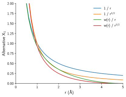
Figure S2: Dependence of a proposed $X_{1}$ functional form according to interatomic distances. A cutoff of 5 Å is used for the weight function $w(r)$.

where $r_{c}$ is a cutoff distance. The weight function was chosen to satisfy two criteria: (1) fast convergence of the descriptor; and (2) scaling of each component of $\mathbf{X}_{1}$ approaching $r^{-3/2}$ to resembles the relationship between entropy and distances in an ideal gas. Figure S2 shows how the combination of the weight function (S4) and the inverse distance $1/r_{ij}$ approximates a dependence of $r_{ij}^{-3/2}$.

In principle, given a large number of neighbors, the unit cell parameters, and $r_{c}$, an input structure $S$ may be reconstructed from $f(S)=\{\mathbf{X}^{(1)}\}$ up to an isometry. ³²

.1.2 Cross terms

As the structure can only be reconstructed from the set of representations of all neighbors, increasing the amount of information in each local environment is desirable. This would also allow us to distinguish between environments containing the same set of nearest-neighbor distances, but different angles. One way to do so is to incorporate distances between atoms in a neighborhood of $i$,

$$X_{ijl}^{(2)}=\frac{\sqrt{w(r_{ij})w(r_{il})}}{r_{jl}},$$ (S5)

which is performed for each neighbor $l$ of atom $j$ in the neighborhood of $i$. The weights $w(r_{ij})$ and $w(r_{il})$ ensure that smaller distances $r_{jl}$ are less important far away from the center of the neighborhood. The square root ensures that $\mathbf{X}_{i}^{(2)}$ has the same scaling and units as $\mathbf{X}_{i}^{(1)}$. The final representation on a per-neighbor basis is

$$\mathbf{X}_{ij}^{(2)}=\left(X_{ij1}^{(2)},\ldots,X_{ijk}^{(2)}\right),$$ (S6)

with the constraint $X_{ij1}^{(2)}\geq\ldots\geq X_{ij(k-1)}^{(2)}$. Finally, the second-order representation term for each atom is given by

$$\mathbf{X}_{i}^{(2)}=\frac{1}{k}\sum_{j}\mathbf{X}_{ij}^{(2)}.$$ (S7)

Where the radial distances $\mathbf{X}_{i}^{(1)}$ already suffice for reconstruction when all $i$’s are considered, the pairwise cross distances $\mathbf{X}_{i}^{(2)}$ may help reconstructing environments only from the vector $\mathbf{X}_{i}=\left(\mathbf{X}_{i}^{(1)},\mathbf{X}_{i}^{(2)}\right)$, even though reconstruction may not be guaranteed for this descriptor. If instead of an average in Eq. (S7) we concatenated all vectors $\mathbf{X}_{ij}^{(2)}$, then reconstruction could be guaranteed within the sphere limited by $r_{c}$. Continuity of this descriptor is only possible when this cutoff $r_{c}$ is smaller than the distance of the central atom to the $k-$th nearest neighbor, as switching between neighbors would create a discontinuity for the aggregated contributions.

.2 Dataset entropy

According to information theory, the entropy $\mathcal{H}$ of a distribution $p(x)$ is defined as

$$\mathcal{H}=-\int p(x)\log p(x)dx,$$ (S8)

where $p(x)$ is the distribution of data points, $\log$ is the natural logarithm, and the value of entropy is integrated over the entire data space $x\in\mathcal{X}$. In our case, using this definition has two problems: (1) it assumes the knowledge of the prior distribution $p(x)$ over the data space; and (2) it requires the integration over the entire configuration space. Obtaining both requires exhaustively sampling the potential energy surfaces (PESes), which is undesirable.

Recently, Perez et al. proposed the use of entropy-maximization schemes for automatic dataset generation for machine learning (ML) interatomic potentials (IPs) ^{35, 49}. To bypass the problems above, the authors approximated the entropy using a classical non-parametric estimation from the literature ³⁴. Up to a constant, that estimate is given by

$$\mathcal{H}\left(\{\mathbf{X}\}\right)=\frac{1}{n}\sum_{i=1}^{n}\log\left(n\min_{j}\left\lVert\mathbf{X}_{i}-\mathbf{X}_{j}\right\rVert\right),$$ (S9)

with $\mathbf{X}_{i}$ the descriptor of atom $i$, $n$ the number of descriptors in the set $\{\mathbf{X}\}$, and $\left\lVert.\right\rVert$ the L₂ norm. One problem with this description is that the nearest-neighbor distance in the descriptor space may not be a good approximation of the distribution density $p(x)$ and strongly depends on the choice of descriptor. Furthermore, the information penalty for overlapping descriptors (i.e., $\left\lVert\mathbf{X}_{i}-\mathbf{X}_{j}\right\rVert\rightarrow 0$) is $\mathcal{H}\rightarrow-\infty$, which may be undesirable. Often, when sampling PESes, oversampling certain configurations is expected, which can pose a problem to a measure of entropy that drastically penalizes any overlap between two points. Finally, the value of entropy is unbounded, assuming any real value. This prevents concrete analogies both with thermodynamics and information theory.

To bypass these problems, we model the distribution of data points $p(x)$ using a kernel density estimation (KDE) and use to quantify the entropy of a dataset. This first estimate is obtained by using a normalized kernel $K_{h}(\mathbf{X},\mathbf{X}_{i})$ with bandwidth $h$ and averaging over all data points in a dataset $\{\mathbf{X}_{i}\}$,

$$p(\mathbf{X})=\frac{1}{n}\sum_{i=1}^{n}K_{h}(\mathbf{X},\mathbf{X}_{i}).$$ (S10)

Then, as sampling the input space $\mathcal{X}$ is undesirable when calculating the integral in Eq. (S8), we propose an empirical estimate³⁴ given by

$$\mathcal{H}\left(\{\mathbf{X}\}\right)=-\frac{1}{n}\sum_{i=1}^{n}\log p(\mathbf{X}_{i}).$$ (S11)

This equation corresponds to the empirical entropy for a set of points. Now, using Eq. (S10) to compute $\log p(\mathbf{X}_{i})$ further simplifies this equation to

$$\mathcal{H}\left(\{\mathbf{X}\}\right)=-\frac{1}{n}\sum_{i=1}^{n}\log\left[\frac{1}{n}\sum_{j=1}^{n}K_{h}(\mathbf{X}_{i},\mathbf{X}_{j})\right],$$ (S12)

To finally compute the entropy, a Gaussian kernel between descriptors can be used,

$$K_{h}(\mathbf{X}_{i},\mathbf{X}_{j})=\exp\left(\frac{-\left\lVert\mathbf{X}_{i}-\mathbf{X}_{j}\right\rVert^{2}}{2h^{2}}\right),$$ (S13)

where $\left\lVert.\right\rVert$ is the $L_{2}$ norm. Along with Equation (S12), the computation of the kernel allows us to measure the information entropy of a given atomistic dataset with a single parameter $h$.

.3 Properties of the entropy

The main difference between Eqs. (S12) and (S9) lies on the fact that overlapping points in the former do not lead to $\mathcal{H}\rightarrow-\infty$, which is desirable when sampling potential energy surfaces. Moreover, appropriate choice of a kernel $K_{h}$ abstracts away from descriptor distances and maps the entropy back to the space of probability distributions. As a consequence, our entropy (S12) exhibits the following properties:

• Bounds: the normalization of the kernel, $0\leq K_{h}(\mathbf{X}_{i},\mathbf{X}_{j})\leq 1$, implies that $1\leq\sum_{j}K_{h}(\mathbf{X}_{i},\mathbf{X}_{j})\leq n$, so $\mathcal{H}$ is bounded between 0 and $\log n$.

• Minimum entropy: $\mathcal{H}=0$ corresponds to a degenerate dataset created with multiple copies of a single $\mathbf{X}_{i}$, thus one that does not provide information about a space $\mathcal{X}$ but only for a single point. This is exactly what one expects from $p(x)\rightarrow\delta(x)$ in Eq. (S8).

• Maximum entropy: $\mathcal{H}=\log n$ corresponds to a dataset with zero overlap between data points, hence conveying maximal information. In information theory, this corresponds to distributions where all outcomes are equally likely.

• Entropy grows with dataset size: Because of the $\log n$ term, datasets composed by non-overlapping data points always bring more information as the training set grows.

• Entropy can decrease as new points are added: In addition to the $\log n$ effect, if new points overlap substantially with the existing dataset, the entropy of the new dataset may be smaller than the entropy of the original dataset.

• Units: because of the reliance on the probability distributions, the entropy has units (nats) and can be used to compare datasets and descriptors. For example, for the same datasets, incomplete descriptors should have lower entropy than complete ones, as the former map two points to the same representation. For the same descriptors, richer datasets should have higher entropy than redundant ones.

These entropy properties correspond exactly to those in the field of information theory and, as a consequence of Eq. (S8), also relate to some of those from statistical mechanics.

.4 Differential entropy

In addition to the dataset entropy from Eq. (S12), one can compute the expected variation in entropy from adding a new point to the dataset even when the distances $\left\lVert\mathbf{X}-\mathbf{X}_{i}\right\rVert$ are not infinite. In information theory, this corresponds to how much information the new data brings to the dataset considering its current distribution of points. Considering an arbitrary point in Eq. (S12), we define the differential entropy $\delta\mathcal{H}$ of adding a point $\mathbf{Y}$ to a dataset $\{\mathbf{X}_{i}\}_{i=1,\ldots,n}$ can be quantified as

$$\delta\mathcal{H}(\mathbf{Y}|\{\mathbf{X}_{i}\})=-\log\left[\sum_{i=1}^{n}K_{h}(\mathbf{Y},\mathbf{X}_{i})\right].$$ (S14)

This form is related to the functional derivative of the information entropy from Eq. (S8) with respect to the probability distribution $p(x)$,

$$\frac{\delta\mathcal{H}}{\delta p(x)}=-1-\log p(x),$$ (S15)

thus representing the sensitivity of the entropy $\mathcal{H}$ with respect to variations of its distribution $p(x)$. In our work, we shift it for convenience by a constant $1-\log n$ (partially due to the normalization of the kernel and $p(x)$) and adopt $\delta\mathcal{H}=\log n-\log p(x)$, as this leads to $\delta\mathcal{H}=0$ for a density estimate of non-overlapping points. Furthermore, the term “differential entropy” is usually employed in information theory to describe the entropy of a continuous probability distribution. In our case, we prefer to reserve this term to the quantity given by $\delta\mathcal{H}$ and avoid using different terms for continuous or discrete probability distributions.

Equation (S14) above has interesting properties for dataset analysis and construction:

• There is no limit to “information novelty”: Contrary to $\mathcal{H}$ in Eq. (S12), $\delta\mathcal{H}$ does not have an upper bound. If the point $\mathbf{Y}$ has near-zero overlap with all points $\{\mathbf{X}_{i}\}$ of the existing dataset — and thus has maximal novelty — then $K_{h}(\mathbf{Y},\mathbf{X}_{i})\rightarrow 0$ and $\delta\mathcal{H}\rightarrow+\infty$.

• Duplicating one isolated point from the training set brings zero information: If a point $\mathbf{Y}$ overlaps perfectly with only one data point in $\{\mathbf{X}_{i}\}$, the sum over kernel values is one and $\delta\mathcal{H}=0$.

• Negative $\delta\mathcal{H}$ implies redundant information: A point that overlaps with multiple points may have the summation over kernel values greater than one, leading to $\delta\mathcal{H}<0$. The latter situation corresponds to points that are overrepresented in the dataset $\{\mathbf{X}_{i}\}$

• Lower bound: the differential entropy has a lower bound $-\log n\leq\delta\mathcal{H}$, where $n$ is the size of the dataset $\{\mathbf{X}\}$. This can only be achieved in the case where $K_{h}(\mathbf{Y},\mathbf{X}_{i})=1$, and represents the scenario where all points overlap. The result can be interpreted as an absolute threshold for dataset redundancy.

With the properties above, it follows that the differential entropy of the points in the training set is always smaller or equal to zero, which allows us to compute uncertainties without arbitrary thresholds.

The entropy of a system can be recovered from the values of $\delta\mathcal{H}$ by

$$\mathcal{H}(\{\mathbf{X}\})=\log n-\frac{1}{n}\sum_{j=1}^{n}\delta\mathcal{H}(\mathbf{X}_{j}|\{\mathbf{X}\}).$$ (S16)

Importantly, however, the differential entropy $\delta\mathcal{H}$ cannot be used to measure the entropy $\mathcal{H}(\{\mathbf{X}_{i}\}_{i=1,\ldots,n+1})$ compared to $\mathcal{H}(\{\mathbf{X}_{i}\}_{i=1,\ldots,n})$ when the point $\mathbf{X}_{n+1}$ is added to $\{\mathbf{X}_{i}\}_{i=1,\ldots,n}$. As the new estimated probability distribution $p(x)$ changes given the knowledge of $\mathbf{X}_{n+1}$, the density $\frac{1}{n}\sum_{j}K_{h}(\mathbf{X}_{i},\mathbf{X}_{j})$ may change when the summation index is allowed to go from 1 to $n+1$ instead of $1$ to $n$.

.5 Entropy in the nearest-neighbors limit

In the limit of non-overlapping points, the sum over kernel values $K_{h}(\mathbf{X}_{i},\mathbf{X}_{j})$ from Eq. (S12) can be simplified to $K_{h}(\mathbf{X}_{i},\mathbf{X}_{i})=1$ plus the nearest neighbor value,

$$\mathcal{H}\left(\{\mathbf{X}\}\right)\approx\log{n}-\frac{1}{n}\sum_{i=1}^{n}\log\left[1+\max_{j\neq i}K_{h}(\mathbf{X}_{i},\mathbf{X}_{j})\right],$$ (S17)

thus resembling the result from Eq. (S9). The assumption of a nearest neighbor dominance expedites the calculation of the entropy. However, the result may not be accurate, as it requires points with small overlap in the descriptor space, an unusual assumption when dealing with PESes. On the other hand, computing all pairwise kernels $K_{h}(\mathbf{X}_{i},\mathbf{X}_{j})$ can be expensive for a large dataset $\{\mathbf{X}\}$. A good compromise is to implement the summation over the neighborhood $\mathcal{N}_{k}$ of $\mathbf{X}_{i}$, which contains the $k$-nearest neighbors of $\mathbf{X}_{i}$,

$$\mathcal{H}\left(\{\mathbf{X}\}\right)\approx-\frac{1}{n}\sum_{i=1}^{n}\log\left[\frac{1}{k}\sum_{\mathbf{X}_{j}\in\mathcal{N}_{k}(\mathbf{X}_{i})}K_{h}(\mathbf{X}_{i},\mathbf{X}_{j})\right],$$ (S18)

and query the $k$-nearest neighbors with average complexity $\mathcal{O}(kd\log N)$, where $N$ is the reference dataset size. Several approximations and nearest neighbors search methods can be employed to obtain the nearest neighbors in the feature space. In the main results of this paper, we used an approach based on nearest neighbors graph, which can handle dataset sizes on the order of millions, and is helpful when performing uncertainty quantification.

The use of approximate nearest neighbors for the computation of $\delta\mathcal{H}$ is analogous to that from $\mathcal{H}$,

$$\delta\mathcal{H}(\mathbf{Y}|\{\mathbf{X}\})\approx-\log\left[\sum_{\mathbf{X}_{j}\in\mathcal{N}_{k}(\mathbf{Y})}K_{h}(\mathbf{Y},\mathbf{X}_{j})\right].$$ (S19)

An immediate consequence of this approximation is that the value of $\delta\mathcal{H}$ is overestimated, as contributions from neighbors outside of the $k$-neighborhood of each vector are neglected. As the values of $k$ increase, $\delta\mathcal{H}$ necessarily decreases, reaching a minimum when the full dataset size is used for its computation. Therefore, when used with the absolute threshold $\delta\mathcal{H}>0$, the approximate $\delta\mathcal{H}$ are conservative estimates of the uncertainty. Some approximate nearest neighbor methods also have recall smaller than 100%, representing the case where some of the true nearest neighbors are not recalled during the query. Although a lower recall could affect the computation of absolute values such as thermodynamic entropies, less accurate $\delta\mathcal{H}$ are still overestimated with respect to an ideal nearest neighbor search. This demonstrates that, despite the approximations of truncating the expansion of $\delta\mathcal{H}$, this value can provide conservative estimates when used as an UQ metric.

.6 Dependence of entropy with the bandwidth

The non-parametric estimation of the information entropy $\mathcal{H}$ described in Eq. (S12) requires fitting a KDE to the data distribution. In the current work, this selection is challenging due to two issues: (1) differences in density lead to changes in the metric space of the descriptors $\mathbf{X}$; and (2) differences in entropy can vary with the choice of bandwidth. Because lower densities (higher atomic volumes) lead to lower distances in the descriptor spaces, we propose a variable bandwidth that decreases with increasing atomic volume,

$$h(V)=a\exp\left(-bV^{2}\right)+c,$$ (S20)

where $a$, $b$, and $c$ are unknown parameters. To estimate these parameters in a self-consistent way, we first performed simulations for the copper Einstein crystal at the NVT ensemble using the spring constant of 34.148 eV/Ų, as described in the LABEL:sec:methods, and for volumes from 6 to 50 ų/atom. The fix ti/spring command in LAMMPS was used with a value of $\lambda$ that ensures that only the harmonic oscillator is considered in the simulation. Then, for each volume, the entropy of the system is computed for a range of entropies, varying from 0.010 to 0.090 Å^-1. As the entropy of the Einstein crystal is independent of the volume, we estimate the values of bandwidth that would keep the entropy reasonably constant across the range of volumes. Figure S8 shows the results of this investigation, and the fitted bandwidth prediction that rescales the (arbitrary) information entropy to the thermodynamically relevant units $k_{B}$/atom.

.7 Dataset diversity

As shown in Fig. 3 of the main paper, the dataset entropy depends on how frequent each environment is sampled in the configuration space. Therefore, entropy values can often reduce even as dataset sizes drastically increase. To create a measure of dataset diversity that is more robust to oversampling, we propose to express the diversity $D$ as

$$D\left(\{\mathbf{X}\}\right)=\log\left[\sum_{i=1}^{n}\frac{1}{\sum_{j=1}^{n}K(\mathbf{X}_{i},\mathbf{X}_{j})}\right]=\log\left[\sum_{i=1}^{n}\exp\left(\delta\mathcal{H}_{i}\right)\right],$$ (S21)

where $\delta\mathcal{H}_{i}=\delta\mathcal{H}(\mathbf{X}_{i}|\{\mathbf{X}\})$. This analytical form is proposed to satisfy the following properties:

• For non-overlapping datasets, $D$ recovers $\mathcal{H}$: this can be demonstrated by verifying that, in datasets where $K(\mathbf{X}_{i},\mathbf{X}_{j})=\delta_{ij}$, $\delta\mathcal{H}_{i}=1,\forall i$ and $D(\{\mathbf{X}\})=H(\{\mathbf{X}\})=\log n$.

• An entirely new data point increases the summation in diversity by one: this follows from the fact that, for a new point $\mathbf{X}_{(n+1)}$ that does not overlap with any of the other points $\mathbf{X}_{i}$, $\delta\mathcal{H}_{(n+1)}=0$.

• $D$ has the same units of $\delta\mathcal{H}$, which is determined by the base of the logarithm, and thus is nats for this work.

• Repeating data points in the training set does not increase its diversity, even if the entropy can be reduced. This follows from the summation of inverse of $p(\mathbf{X}_{i})$, which approximately re-weights the distribution of data points based on their frequency according to other points.

Within this definition, the diversity $D$ of a dataset represents the coverage of the configuration space. However, it does not express the same value as $\log n$, the maximum information entropy. Whereas $\log n$ is agnostic to the coverage of the space, $D$ attempts to quantify exactly how many unique points are present in the system. For example, a degenerate system with $\mathcal{H}=0$ also has $D=0$ regardless of $\log n$.

.8 Toy examples for QUESTS

.8.1 2D visualization of the entropy

To visualize the concepts of entropy and distributions, we sampled 100 points in a two-dimensional space from a 2D Gaussian with mean zero and covariance matrix equal to the identity. Then, we computed the values of $p(x)$ from a KDE and its corresponding $\delta\mathcal{H}$ for each point on the 2D grid. Figures S3 and S4 show how the entropy $H$ and the differential entropy $\delta\mathcal{H}$ behave with different distributions, bandwidths, and rescaling. If the objective was to reproduce the original Gaussian, as in a standard KDE, the choice of higher bandwidths (Fig. S3c) better approximates the actual distribution. While this example is more difficult to visualize in a high-dimensional space of atomistic environments, the distribution plots illustrate the analogous result that would happen to them.

.8.2 Visualization and distance for the atomistic representation

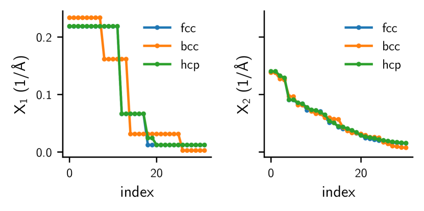
Figure S5: Visualization of the $\mathbf{X}_{1}$ and $\mathbf{X}_{2}$ representation for FCC, BCC, and HCP structures. The small differences between FCC and HCP can be seen only at neighbors further away from the origin.

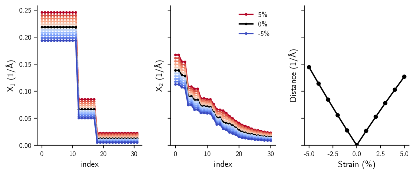
Figure S6: Behavior of the $\mathbf{X}_{1}$ (left) and $\mathbf{X}_{2}$ (middle) representation for an FCC structure under strain between -5% (expansion, blue) and 5% (compression, red). The Euclidean distance between the strained and reference structure is shown on the right. Within this range of uniform strains and this structure, the distance varies linearly.

The representation proposed in this work was created on a per-environment basis, with radial distances and cross distances, as explained in Section II.1 above and shown in Fig. S1. The representation can be visualized in a single plot and used to differentiate between standard crystal structures, such as BCC, FCC, and HCP (Fig. S5). This descriptor can also be used upon modification of the original structure, such as strain. In Fig. S6, an FCC structure is strained between -5% and 5%, and the representation is visualized according to the applied strain. Interestingly, the distance between the descriptors and the applied strain varies near-linearly within this range.

.8.3 Information entropy and heat capacity

Although the information entropy can be rescaled using the values of the bandwidth, it is relevant to verify whether they follow the same seen in physics models. One of such models is the Debye’s model, which considers atoms interacting via harmonic potentials as a model for phonons and heat capacity. To obtain classical MD trajectories that match the physics from the Debye model (and the zero-point energy in quantum harmonic oscillators), we used the quantum thermal bath (QTB) implemented in LAMMPS.⁷⁸ We simulated a $10\times 10\times 10$ box of particles with the FCC structure, unit cell parameter of 3.645 Å, and mass of 62.5 g/mol. The bond terms are determined by the spring constant $k=1.0$ eV/Ų and an equilibrium distance of $2.5775$ Å. Bonds are created for particles that are between 2.0 and 3.0 Å apart. Then, the simulation is performed using a QTB at constant temperature, varying from 10 to 1000 K, $f_{\mathrm{max}}=120$ ps^-1, $N_{f}=100$, constant volume. The simulation was performed with an equilibration run of 300 ps and a production run of 100 ps using a timestep of 2 fs. The results are shown in Fig. S7. Although the entropy was obtained with a constant, low value of bandwidth (0.015 Å^-1), the entropy of a fitted Debye model matches closely that from the extracted simulations. Importantly, the entropy does not approach zero at 0 K due to the residual motion from the simulations that mimic the behavior of the zero-point energy.

.8.4 Information entropy upon denoising

To exemplify how the entropy $\mathcal{H}$ and the descriptors can be used to quantify information within atomistic systems, we analyzed trajectories with decreasing diversity of atomic environments from Ref. 79. Because the deviations of the atoms from their ideal lattice sites were removed with a denoising method to enable phase classification, we expect the values of $\mathcal{H}$ to decrease accordingly. To validate this intuition for $\mathcal{H}$, we computed the information entropy of four denoised phases of copper, as shown in Fig S9. As vibrational motion is removed from the system, the values of $\mathcal{H}$ for the crystalline phases FCC, BCC, and HCP decrease until reaching zero.⁷⁹ On the other hand, the liquid phase cannot be fully denoised, and the residual disorder is manifested in a higher information entropy value. This example suggests that the connection between configurational degrees of freedom and information $\mathcal{H}$ can be interpreted as similar to the information entropy.

.8.5 Information entropy and Lindemann’s melting criterion

The Lindemann melting criterion is a well-known estimate for the melting point of materials.⁸⁰ According to this estimate, melting often happens when the ratio between the root mean square displacement (RMSD) of atoms with respect to their ideal lattice positions and the ideal interatomic distances approaches a constant factor, often around 0.10 for several metals. To verify if our method could reproduce these results, we gradually added noise to the positions of prototypical FCC, BCC, and HCP crystal structures. To obtain a statistically meaningful result, we employed a $25\times 25\times 25$ supercell for each of the structures, thus creating structures with 15,625 atoms. Then, for each level of noise, we computed the RMSD with respect to the ideal lattice sites, and the entropy of the noisy configuration. When a bandwidth of 0.057 Å^-1 is used for the chosen volumes (Fig. S8), the resulting entropy is shown in Fig. S10. The results show that the entropy increases rapidly with the RMSD, and reaches values around 0.2 to 0.5 $k_{B}$ with a normalized RMSD between 0.1 and 0.125. As typical entropies of solids prior to melting are around this range of 0.2 to 0.5 $k_{B}$, considering the entropy of a liquid around 1.3 $k_{B}$ and melting entropies between 0.8 and 1.1 $k_{B}$, this result reproduces the intuition behind Lindemann’s melting rule based on the entropy values. While many other factors are responsible for melting and the Lindemann criterion is a rough approximation, this toy example shows that the addition of noise to the system leads to entropy values compatible with expected ranges.

Supplementary Figures

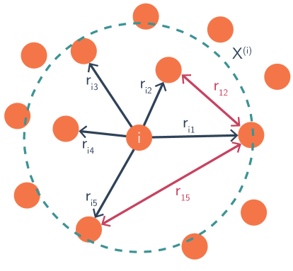
Figure S1: Visualization of the distances used to create the $\mathbf{X}_{1}$ and $\mathbf{X}_{2}$ representation.

Figure S3: 2D example of the KDE, bandwidth, and entropy. a, estimated $p(x)$ for a set of points (marked with x). b, the values of $p(x)$ can be mapped directly to $\delta\mathcal{H}$. This creates a common reference of $\delta\mathcal{H}>0$ for points “outside” of the training set, shown here in red, and $\delta\mathcal{H}<0$ for points “inside” the training set, shown in blue. c, effects of the bandwidth in estimating the probability distribution. A large bandwidth estimates the values as a single Gaussian, whereas a small bandwidth considers each point individually. d, effects of rescaling the coordinates of a distribution by a factor $f$ in the entropy $H$. Denser distributions lead to lower entropy, whereas larger spread relates to higher entropy if the bandwidth is kept constant.

Figure S4: 2D example of distributions with increasing entropy. The first eight distributions were generated randomly, then sorted according to their entropy. This provides a visual guide to interpreting values of lower entropy as more concentrated data points and higher entropy as larger spread. A regular occupation of the (2D) configuration space (bottom right) leads to the highest entropy among all examples. The color follows the same scale as S3b, with red points having $\delta\mathcal{H}>0$ and blue points having $\delta\mathcal{H}<0$.

Figure S7: Information entropy of particles interacting via harmonic bonds under a quantum thermal bath (QTB). At zero temperature, the entropy does not go to zero to simulate the effects of the zero-point energy. A fitted Debye model is shown with a dashed orange line.

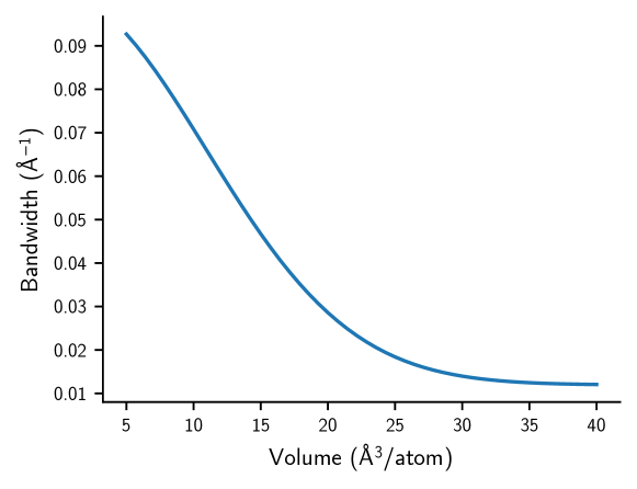
Figure S8: Proposed dependence of the kernel bandwidth with the volume. The bandwidth saturates at high volumes to ensure that residual information is captured from the data despite the non-thermodynamic behavior.

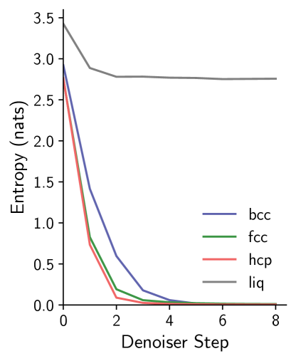
Figure S9: Information entropy of four phases of copper (FCC, HCP, BCC, and liquid) for the denoised trajectories from Ref. 79 from the main paper.

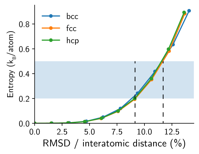
Figure S10: Root mean square deviation (RMSD) of atoms in FCC, BCC, and HCP structures, and their corresponding entropies calculated with QUESTS. The shaded area represents typical solid entropies prior to melting, and intersects the computed curves between 10–12.5% RMSD/interatomic distances, thus reproducing the Lindemann melting rule.

Figure S16: Information gap for all rMD17 molecules as a function of training set size. The gap is defined as the asymptotic value of the information entropy minus the entropy value at a given number of samples. These curves show that, at a typical constant number of samples, the information gap varies substantially across molecules.

References

- Jaynes [1957] E. T. Jaynes, Information theory and statistical mechanics, Physical Review 106, 620 (1957).
- Shannon [1948] C. E. Shannon, A mathematical theory of communication, The Bell System Technical Journal 27, 379 (1948).
- Shwartz-Ziv and Tishby [2017] R. Shwartz-Ziv and N. Tishby, Opening the black box of deep neural networks via information, arXiv:1703.00810 (2017).
- Karplus and Kushick [1981] M. Karplus and J. N. Kushick, Method for estimating the configurational entropy of macromolecules, Macromolecules 14, 325 (1981).
- Morris and Ho [1995] J. R. Morris and K. M. Ho, Calculating Accurate Free Energies of Solids Directly from Simulations, Physical Review Letters 74, 940 (1995).
- Van Siclen [1997] C. D. Van Siclen, Information entropy of complex structures, Physical Review E 56, 5211 (1997).
- Vink and Barkema [2002] R. L. C. Vink and G. T. Barkema, Configurational Entropy of Network-Forming Materials, Physical Review Letters 89, 076405 (2002).
- Killian et al. [2007] B. J. Killian, J. Yundenfreund Kravitz, and M. K. Gilson, Extraction of configurational entropy from molecular simulations via an expansion approximation, The Journal of Chemical Physics 127, 024107 (2007).
- Fultz [2010] B. Fultz, Vibrational thermodynamics of materials, Progress in Materials Science 55, 247 (2010).
- Gao and Widom [2018] M. C. Gao and M. Widom, Information Entropy of Liquid Metals, The Journal of Physical Chemistry B 122, 3550 (2018).
- Mac Fhionnlaoich and Guldin [2020] N. Mac Fhionnlaoich and S. Guldin, Information Entropy as a Reliable Measure of Nanoparticle Dispersity, Chemistry of Materials 32, 3701 (2020).
- Sutton and Levchenko [2020] C. Sutton and S. V. Levchenko, First-Principles Atomistic Thermodynamics and Configurational Entropy, Frontiers in Chemistry 8 (2020).
- Huang and Widom [2022] Y. Huang and M. Widom, Vibrational Entropy of Crystalline Solids from Covariance of Atomic Displacements, Entropy 24, 618 (2022).
- Wallace [1987] D. C. Wallace, Correlation entropy in a classical liquid, Physics Letters A 122, 418 (1987).
- Baranyai and Evans [1989] A. Baranyai and D. J. Evans, Direct entropy calculation from computer simulation of liquids, Physical Review A 40, 3817 (1989).
- Torrens [1972] I. Torrens, Interatomic Potentials (Academic Press, New York, 1972).
- Frenkel and Smit [2002] D. Frenkel and B. Smit, Understanding molecular simulation: from algorithms to applications (Academic Press San Diego, 2002).
- Behler and Parrinello [2007] J. Behler and M. Parrinello, Generalized Neural-Network Representation of High-Dimensional Potential-Energy Surfaces, Physical Review Letters 98, 146401 (2007).
- Bartók et al. [2010] A. P. Bartók, M. C. Payne, R. Kondor, and G. Csányi, Gaussian Approximation Potentials: The Accuracy of Quantum Mechanics, without the Electrons, Physical Review Letters 104, 136403 (2010), arXiv:0910.1019 .
- Behler [2015] J. Behler, Constructing high-dimensional neural network potentials: A tutorial review, Int. J. Quantum Chem. 115, 1032 (2015).
- Thompson et al. [2015] A. P. Thompson, L. P. Swiler, C. R. Trott, S. M. Foiles, and G. J. Tucker, Spectral neighbor analysis method for automated generation of quantum-accurate interatomic potentials, Journal of Computational Physics 285, 316 (2015).
- Chmiela et al. [2017] S. Chmiela, A. Tkatchenko, H. E. Sauceda, I. Poltavsky, K. T. Schütt, and K.-R. Müller, Machine learning of accurate energy-conserving molecular force fields, Science Advances 3, 10.1126/sciadv.1603015 (2017).
- Zhang et al. [2018] L. Zhang, J. Han, H. Wang, R. Car, and E. Weinan, Deep potential molecular dynamics: a scalable model with the accuracy of quantum mechanics, Physical Review Letters 120, 143001 (2018).
- Mueller et al. [2020] T. Mueller, A. Hernandez, and C. Wang, Machine learning for interatomic potential models, The Journal of Chemical Physics 152, 050902 (2020).
- Manzhos and Carrington [2021] S. Manzhos and T. Carrington, Neural Network Potential Energy Surfaces for Small Molecules and Reactions, Chemical Reviews 121, 10187 (2021).
- Unke et al. [2021] O. T. Unke, S. Chmiela, H. E. Sauceda, M. Gastegger, I. Poltavsky, K. T. Schütt, A. Tkatchenko, and K.-R. Müller, Machine Learning Force Fields, Chemical Reviews 121, 10142 (2021).
- Batzner et al. [2022] S. Batzner, A. Musaelian, L. Sun, M. Geiger, J. P. Mailoa, M. Kornbluth, N. Molinari, T. E. Smidt, and B. Kozinsky, E(3)-equivariant graph neural networks for data-efficient and accurate interatomic potentials, Nature Communications 13, 2453 (2022).
- Batatia et al. [2022] I. Batatia, D. P. Kovacs, G. Simm, C. Ortner, and G. Csanyi, MACE: Higher Order Equivariant Message Passing Neural Networks for Fast and Accurate Force Fields, in Advances in Neural Information Processing Systems, Vol. 35, edited by S. Koyejo, S. Mohamed, A. Agarwal, D. Belgrave, K. Cho, and A. Oh (Curran Associates, Inc., 2022) pp. 11423–11436.
- Schwalbe-Koda et al. [2021] D. Schwalbe-Koda, A. R. Tan, and R. Gómez-Bombarelli, Differentiable sampling of molecular geometries with uncertainty-based adversarial attacks, Nature Communications 12, 5104 (2021).
- Fu et al. [2022] X. Fu, Z. Wu, W. Wang, T. Xie, S. Keten, R. Gomez-Bombarelli, and T. Jaakkola, Forces are not Enough: Benchmark and Critical Evaluation for Machine Learning Force Fields with Molecular Simulations, arXiv:2210.07237 10.48550/arXiv.2210.07237 (2022), arXiv:2210.07237 .
- Vita and Schwalbe-Koda [2023] J. A. Vita and D. Schwalbe-Koda, Data efficiency and extrapolation trends in neural network interatomic potentials, Machine Learning: Science and Technology 4, 035031 (2023).
- Widdowson and Kurlin [2022] D. Widdowson and V. Kurlin, Resolving the data ambiguity for periodic crystals, Advances in Neural Information Processing Systems (NeurIPS 2022) 35, 24625 (2022).
- Schwalbe-Koda et al. [2023a] D. Schwalbe-Koda, D. E. Widdowson, T. A. Pham, and V. A. Kurlin, Inorganic synthesis-structure maps in zeolites with machine learning and crystallographic distances, Digital Discovery 2, 1911 (2023a).
- Beirlant et al. [1997] J. Beirlant, E. J. Dudewicz, L. Györfi, E. C. Van der Meulen, et al., Nonparametric entropy estimation: An overview, International Journal of Mathematical and Statistical Sciences 6, 17 (1997).
- Karabin and Perez [2020] M. Karabin and D. Perez, An entropy-maximization approach to automated training set generation for interatomic potentials, The Journal of Chemical Physics 153 (2020).
- Mishin et al. [2001] Y. Mishin, M. Mehl, D. Papaconstantopoulos, A. Voter, and J. Kress, Structural stability and lattice defects in copper: Ab initio, tight-binding, and embedded-atom calculations, Physical Review B 63, 224106 (2001).
- Smirnov [2021] N. A. Smirnov, Relative stability of Cu, Ag, and Pt at high pressures and temperatures from ab initio calculations, Physical Review B 103, 064107 (2021).
- Ravelo and Baskes [1997] R. Ravelo and M. Baskes, Equilibrium and Thermodynamic Properties of Grey, White, and Liquid Tin, Physical Review Letters 79, 2482 (1997).
- Chung et al. [2022] H. W. Chung, R. Freitas, G. Cheon, and E. J. Reed, Data-centric framework for crystal structure identification in atomistic simulations using machine learning, Physical Review Materials 6, 043801 (2022).
- Justo et al. [1998] J. F. Justo, M. Z. Bazant, E. Kaxiras, V. V. Bulatov, and S. Yip, Interatomic potential for silicon defects and disordered phases, Physical review B 58, 2539 (1998).
- Tersoff [1989] J. Tersoff, Modeling solid-state chemistry: Interatomic potentials for multicomponent systems, Physical review B 39, 5566 (1989).
- Faken and Jónsson [1994] D. Faken and H. Jónsson, Systematic analysis of local atomic structure combined with 3d computer graphics, Computational Materials Science 2, 279 (1994).
- Mendelev et al. [2010] M. Mendelev, M. Rahman, J. Hoyt, and M. Asta, Molecular-dynamics study of solid–liquid interface migration in fcc metals, Modelling and Simulation in Materials Science and Engineering 18, 074002 (2010).
- Stukowski [2012] A. Stukowski, Structure identification methods for atomistic simulations of crystalline materials, Modelling and Simulation in Materials Science and Engineering 20, 045021 (2012).
- Turnbull [2004] D. Turnbull, Formation of Crystal Nuclei in Liquid Metals, Journal of Applied Physics 21, 1022 (2004).
- Vinet et al. [2002] B. Vinet, L. Magnusson, H. Fredriksson, and P. J. Desré, Correlations between Surface and Interface Energies with Respect to Crystal Nucleation, Journal of Colloid and Interface Science 255, 363 (2002).
- Kaptay [2020] G. Kaptay, A coherent set of model equations for various surface and interface energies in systems with liquid and solid metals and alloys, Advances in Colloid and Interface Science 283, 102212 (2020).
- Bernstein et al. [2019] N. Bernstein, G. Csányi, and V. L. Deringer, De novo exploration and self-guided learning of potential-energy surfaces, npj Computational Materials 5, 99 (2019).
- de Oca Zapiain et al. [2022] D. M. de Oca Zapiain, M. A. Wood, N. Lubbers, C. Z. Pereyra, A. P. Thompson, and D. Perez, Training data selection for accuracy and transferability of interatomic potentials, npj Computational Materials 8, 10.1038/s41524-022-00872-x (2022).
- Qi et al. [2023] J. Qi, T. W. Ko, B. C. Wood, T. A. Pham, and S. P. Ong, Robust training of machine learning interatomic potentials with dimensionality reduction and stratified sampling, arXiv:2307.13710 (2023).
- Chen and Ong [2022] C. Chen and S. P. Ong, A universal graph deep learning interatomic potential for the periodic table, Nature Computational Science 2, 718 (2022).
- Merchant et al. [2023] A. Merchant, S. Batzner, S. S. Schoenholz, M. Aykol, G. Cheon, and E. D. Cubuk, Scaling deep learning for materials discovery, Nature , 80 (2023).
- Batatia et al. [2023] I. Batatia, P. Benner, Y. Chiang, A. M. Elena, D. P. Kovács, J. Riebesell, X. R. Advincula, M. Asta, W. J. Baldwin, N. Bernstein, et al., A foundation model for atomistic materials chemistry, arXiv:2401.00096 (2023).
- Rowe et al. [2020] P. Rowe, V. L. Deringer, P. Gasparotto, G. Csányi, and A. Michaelides, An accurate and transferable machine learning potential for carbon, The Journal of Chemical Physics 153 (2020).
- Li et al. [2023] K. Li, D. Persaud, K. Choudhary, B. DeCost, M. Greenwood, and J. Hattrick-Simpers, Exploiting redundancy in large materials datasets for efficient machine learning with less data, Nature Communications 14, 7283 (2023).
- Schwalbe-Koda et al. [2023b] D. Schwalbe-Koda, N. Govindarajan, and J. Varley, Controlling neural network extrapolation enables efficient and comprehensive sampling of coverage effects in catalysis, ChemRxiv 10.26434/chemrxiv-2023-f6l23 (2023b).
- Smith et al. [2017] J. S. Smith, O. Isayev, and A. E. Roitberg, ANI-1: an extensible neural network potential with DFT accuracy at force field computational cost, Chemical Science 8, 3192 (2017), arXiv:1610.08935 .
- Hu et al. [2022] Y. Hu, J. Musielewicz, Z. W. Ulissi, and A. J. Medford, Robust and scalable uncertainty estimation with conformal prediction for machine-learned interatomic potentials, Machine Learning: Science and Technology 3, 045028 (2022).
- Tan et al. [2023] A. R. Tan, S. Urata, S. Goldman, J. C. Dietschreit, and R. Gómez-Bombarelli, Single-model uncertainty quantification in neural network potentials does not consistently outperform model ensembles, npj Computational Materials 9, 225 (2023).
- Glielmo et al. [2018] A. Glielmo, C. Zeni, and A. De Vita, Efficient nonparametric n-body force fields from machine learning, Physical Review B 97, 184307 (2018).
- Vandermause et al. [2020] J. Vandermause, S. B. Torrisi, S. Batzner, Y. Xie, L. Sun, A. M. Kolpak, and B. Kozinsky, On-the-fly active learning of interpretable Bayesian force fields for atomistic rare events, npj Computational Materials 6, 1 (2020).
- Zhu et al. [2023] A. Zhu, S. Batzner, A. Musaelian, and B. Kozinsky, Fast uncertainty estimates in deep learning interatomic potentials, The Journal of Chemical Physics 158 (2023).
- Pozdnyakov et al. [2020] S. N. Pozdnyakov, M. J. Willatt, A. P. Bartók, C. Ortner, G. Csányi, and M. Ceriotti, Incompleteness of atomic structure representations, Physical Review Letters 125, 166001 (2020).
- Lam et al. [2015] S. K. Lam, A. Pitrou, and S. Seibert, Numba: A llvm-based python jit compiler, in Proceedings of the Second Workshop on the LLVM Compiler Infrastructure in HPC (2015) pp. 1–6.
- Virtanen et al. [2020] P. Virtanen, R. Gommers, T. E. Oliphant, M. Haberland, T. Reddy, D. Cournapeau, E. Burovski, P. Peterson, W. Weckesser, J. Bright, S. J. van der Walt, M. Brett, J. Wilson, K. J. Millman, N. Mayorov, A. R. J. Nelson, E. Jones, R. Kern, E. Larson, C. J. Carey, İ. Polat, Y. Feng, E. W. Moore, J. VanderPlas, D. Laxalde, J. Perktold, R. Cimrman, I. Henriksen, E. A. Quintero, C. R. Harris, A. M. Archibald, A. H. Ribeiro, F. Pedregosa, P. van Mulbregt, and SciPy 1.0 Contributors, SciPy 1.0: Fundamental Algorithms for Scientific Computing in Python, Nature Methods 17, 261 (2020).
- Thompson et al. [2022] A. P. Thompson, H. M. Aktulga, R. Berger, D. S. Bolintineanu, W. M. Brown, P. S. Crozier, P. J. in ’t Veld, A. Kohlmeyer, S. G. Moore, T. D. Nguyen, R. Shan, M. J. Stevens, J. Tranchida, C. Trott, and S. J. Plimpton, LAMMPS - a flexible simulation tool for particle-based materials modeling at the atomic, meso, and continuum scales, Comp. Phys. Comm. 271, 108171 (2022).
- Freitas et al. [2016] R. Freitas, M. Asta, and M. De Koning, Nonequilibrium free-energy calculation of solids using lammps, Computational Materials Science 112, 333 (2016).
- Piessens et al. [2012] R. Piessens, E. de Doncker-Kapenga, C. W. Überhuber, and D. K. Kahaner, QUADPACK: a subroutine package for automatic integration, Vol. 1 (Springer Science & Business Media, 2012).
- Pedregosa et al. [2011] F. Pedregosa, G. Varoquaux, A. Gramfort, V. Michel, B. Thirion, O. Grisel, M. Blondel, P. Prettenhofer, R. Weiss, V. Dubourg, J. Vanderplas, A. Passos, D. Cournapeau, M. Brucher, M. Perrot, and E. Duchesnay, Scikit-learn: Machine learning in Python, Journal of Machine Learning Research 12, 2825 (2011).
- Schneider and Stoll [1978] T. Schneider and E. Stoll, Molecular-dynamics study of a three-dimensional one-component model for distortive phase transitions, Physical Review B 17, 1302 (1978).
- Nosé [1984] S. Nosé, A unified formulation of the constant temperature molecular dynamics methods, The Journal of chemical physics 81, 511 (1984).
- Hoover [1985] W. G. Hoover, Canonical dynamics: Equilibrium phase-space distributions, Physical review A 31, 1695 (1985).
- Zepeda-Ruiz et al. [2017] L. A. Zepeda-Ruiz, A. Stukowski, T. Oppelstrup, and V. V. Bulatov, Probing the limits of metal plasticity with molecular dynamics simulations, Nature 550, 492 (2017).
- Kingma and Ba [2015] D. Kingma and J. Ba, Adam: A method for stochastic optimization, in International Conference on Learning Representations (ICLR) (San Diego, CA, USA, 2015).
- Reddi et al. [2018] S. J. Reddi, S. Kale, and S. Kumar, On the convergence of adam and beyond, in International Conference on Learning Representations (2018).
- Chase [1998] M. Chase, NIST-JANAF Thermochemical Tables, 4th Edition (American Institute of Physics, 1998).
- Dong et al. [2011] W. Dong, C. Moses, and K. Li, Efficient k-nearest neighbor graph construction for generic similarity measures, in Proceedings of the 20th International Conference on World Wide Web (2011) pp. 577–586.
- Dammak et al. [2009] H. Dammak, Y. Chalopin, M. Laroche, M. Hayoun, and J.-J. Greffet, Quantum thermal bath for molecular dynamics simulation, Physical Review Letters 103, 190601 (2009).
- Hsu et al. [2023] T. Hsu, B. Sadigh, N. Bertin, C. W. Park, J. Chapman, V. Bulatov, and F. Zhou, Score-based denoising for atomic structure identification, arXiv:2212.02421 (2023).
- Lindemann [1910] F. A. Lindemann, über die berechnung molekularer eigenfrequenzen, Physikalische Zeitschrift 11, 609 (1910).