Neutrinoless double beta decay in the minimal type-I seesaw model: mass-dependent nuclear matrix element, current limits and future sensitivities

Abstract

In this work we discuss the neutrino mass dependent nuclear matrix element (NME) of the neutrinoless double beta decay process and derive the limit on the parameter space of the minimal Type-I seesaw model from the current available experimental data as well as the future sensitivities from the next-generation experiments. Both the explicit many-body calculations and naive extrapolations of the mass dependent NME are employed in the current work. The uncertainties of the theoretical nuclear structure models are taken into account. By combining the latest experimental data from ⁷⁶Ge-based experiments, GERDA and MAJORANA, the ¹³⁰Te-based experiment, CUORE and the ¹³⁶Xe-based experiments, KamLAND-Zen and EXO-200, the bounds on the parameter space of the minimal Type-I seesaw model are obtained and compared with the limits from other experimental probes. Sensitivities for future experiments utilizing ⁷⁶Ge-based (LEGEND-1000), ⁸²Se-based (SuperNEMO), ¹³⁰Te based (SNO+II) and ¹³⁶Xe-based (nEXO), with a ten-year exposure, are also derived.

1 Introduction

Neutrinos, as the building blocks of the Standard Model (SM), are the most mysterious fermion of the fundamental particles. The recent groundbreaking discovery of neutrino oscillations Kajita:2016cak ; McDonald:2016ixn has revealed that neutrinos are massive, but their masses are significantly smaller than those of other charged fermions. The nature of electric neutrality allows for the possibility of neutrinos being Majorana fermions, which opens up the potential for explaining the smallness of neutrino masses via the seesaw mechanisms Xing:2020ijf . There are three distinct types of seesaw mechanisms according to the different SM group representations of the right-handed neutrinos (RHNs) and/or Higgs particles Minkowski:1977sc ; Yanagida:1979as ; Gell-Mann:1979vob ; Glashow:1979nm ; Mohapatra:1979ia ; Konetschny:1977bn ; Magg:1980ut ; Schechter:1980gr ; Cheng:1980qt ; Mohapatra:1980yp ; Lazarides:1980nt ; Foot:1988aq . The most popular realization is the canonical type-I seesaw mechanism Minkowski:1977sc ; Yanagida:1979as ; Gell-Mann:1979vob ; Glashow:1979nm ; Mohapatra:1979ia , which introduces at least two SM-singlet Majorana RHNs Frampton:2002qc ; Xing:2020ald ; Guo:2006qa . The active neutrino masses are obtained by diagnolizing the entire neutrino mass matrices and their smallness is attributed to the heavy masses of Majorana RHNs. The models of seesaw mechanisms have far-reaching consequences, particularly in terms of lepton number violation processes in the field of particle and nuclear physics. These include the neutrinoless double beta decay ($0\nu\beta\beta$) process  Bilenky:2014uka ; Dolinski:2019nrj ; Agostini:2022zub ; Engel:2016xgb ; Yao:2021wst , the lepton number violating decays of $K$ or charmed mesons Chun:2019nwi ; Isidori:2014rba and the search for lepton number violating signals at colliders Cai:2017mow . These phenomena provide valuable insights into the nature of neutrino masses and new physics beyond the SM.

The double beta decay is an extremely rare process in the universe, governed by the strong nuclear pairing force that enhances the stability of even-even nuclei compared to odd-odd nuclei Engel:2016xgb ; Yao:2021wst . A unique mode of the double beta decay without the emission of neutrinos, known as the $0\nu\beta\beta$, is of utmost significance since it holds the key to unraveling the mystery of whether neutrinos are their own antiparticles, and thus being a direct probe of the Majorana nature of neutrinos. Experimental searches for the $0\nu\beta\beta$ have been actively conducted worldwide Bilenky:2014uka ; Dolinski:2019nrj ; Agostini:2022zub , with the aim of detecting this extremely rare process and shedding light on the fundamental properties of neutrinos. The results of the $0\nu\beta\beta$ searches have been reported in various experiments using different isotopes, including ¹³⁶Xe-based experiments KamLAND-Zen KamLAND-Zen:2012mmx ; KamLAND-Zen:2016pfg ; KamLAND-Zen:2022tow and EXO-200 EXO-200:2012pdt ; EXO-200:2014ofj ; EXO:2017poz ; EXO-200:2019rkq , ⁷⁶Ge-based experiments GERDA GERDA:2013vls ; Agostini:2017iyd ; GERDA:2018pmc ; GERDA:2019ivs ; GERDA:2020xhi and MAJORANA Majorana:2017csj ; Majorana:2019nbd ; Majorana:2022udl , ¹³⁰Te-based experiment, CUORE CUORE:2017tlq ; CUORE:2019yfd ; CUORE:2021mvw , and experiments using other isotopes such as ⁴⁸Ca Brudanin:2000in ; Ogawa:2004fy ; NEMO-3:2016mvr , ⁸²Se Arnold:2018tmo ; NEMO:2005xxi , ¹⁰⁰Mo Ejiri:2001fx ; NEMO:2005xxi ; NEMO-3:2013pwo ; NEMO-3:2015jgm ; Alenkov:2019jis , ¹¹⁶Cd NEMO-3:2016zfx , and ¹⁵⁰Nd NEMO:2008kpp ; NEMO-3:2016qxo . The most stringent lower limits on the $0\nu\beta\beta$ half-lives of ⁷⁶Ge, ¹³⁵Xe, and ¹³⁰Te are derived at the levels of approximately $10^{25}$ to $10^{26}$ years, while the limits for the other isotopes are at the levels of $10^{24}$ years or below. By taking account of the large spread of the nuclear matrix elements (NMEs), these lower limits on half-lives can be converted to corresponding upper limits on the effective light Majorana neutrino mass, ranging from around 50 meV to several eV Bilenky:2014uka ; Dolinski:2019nrj ; Agostini:2022zub ; Pompa:2023jxc .

In the framework of the Type-I seesaw model, the $0\nu\beta\beta$ process is directly affected by the masses of light and heavy neutrinos within the neutrino propagator, commonly known as the neutrino mass mechanism. Apart from the common phase space factor, the half-lives of the $0\nu\beta\beta$ depend on both the lepton part of the decay rate, denoted as the effective neutrino mass, and the nuclear part, represented by the NMEs. The observation or non-observation of the $0\nu\beta\beta$ with high sensitivity could provide crucial insights and impose stringent constraints on the parameter space of the seesaw mechanism. In our previous study, as shown in Ref. Fang:2021jfv , we have employed the combined effective neutrino mass $m_{\rm eff}$ of the $0\nu\beta\beta$ in the seesaw model by using the empirical mass-dependent relation of the NMEs, and established the bounds on the parameter space given a particular upper limit of $m_{\rm eff}$. In the current study we shall extend to the constraints on the minimal Type I seesaw model Frampton:2002qc ; Xing:2020ald ; Guo:2006qa from the current and future $0\nu\beta\beta$ experimental results. We present a calculation of the mass dependent NMEs from the nuclear many body approach of the quasi-particle random phase approximation (QRPA). Given that a consensus on the convergence of various many-body methods has yet to be achieved, we also compile the current available calculation results of NMEs from light and heavy Majorana neutrino exchanges, and construct the mass-dependent NMEs from the Interacting Boson Model (IBM), Covariant Density Functional Theory (CDFT) and Interacting Shell Model (ISM) using the empirical interpolation relation Faessler:2014kka . By using the model spread from different many body approaches and considering the correlation among the NMEs of different Majorana neutrino masses, we derive the constraints on the parameter space of the minimal Type-I seesaw model from the current $0\nu\beta\beta$ data and compare with the limits from other experimental probes. We also present the sensitivities on the parameter space from the next generation experiments.

The current work is arranged as follows. In Sec. 2, we introduce the theoretical frameworks for both the nuclear and particle sides, and then an analysis of the mass-dependent NME calculations. In Sec. 3, we focus on the constraints on the minimal type-I seesaw model parameters from current experiments and the corresponding sensitive ranges from future $0\nu\beta\beta$ experiments. The last section consists of the conclusions and outlook.

2 Theoretical Framework

In this section we present the general framework of the $0\nu\beta\beta$ in the type-I seesaw model with two RHNs (i.e., the minimal type-I seesaw model). We first introduce the seesaw relation and the effective neutrino mass, and then present the mass-dependent nuclear matrix elements (NMEs) from the QRPA model. Meanwhile, we also compile the NMEs of exchanging the light and heavy Majorana neutrinos from the literature, and construct the mass-dependent NMEs from other nuclear many body models, such as IBM, CDFT, and ISM, using an empirical interpolation relation Faessler:2014kka .

2.1 The Seesaw relations and the effective neutrino mass

In the current work, we consider the relevant Lagrangian for the minimal type-I seesaw model as given by King:1999mb ; Frampton:2002qc ; Guo:2006qa ; Xing:2020ald

$$\mathcal{L}=\mathcal{L}_{\mathrm{SM}}-\left(Y_{\alpha}\overline{L_{\alpha}}\Phi N_{\mathrm{R}}+\frac{1}{2}\overline{N_{\mathrm{R}}^{c}}M_{R}N_{\mathrm{R}}+\rm{h.c.}\right),$$ (1)

where $L_{\alpha}=(\nu_{\alpha{\rm L}},l_{\alpha{\rm L}})^{\mathrm{T}}(\alpha=e,\mu,\tau)$ are the left-handed lepton doublets, $N_{\mathrm{R}}$ denotes the two SM singlets of RHNs and $\Phi$ is the Higgs doublet. $Y_{\alpha}$ is the $3\times 2$ neutrino Yukawa coupling matrix and $M_{\mathrm{R}}$ is the $2\times 2$ Majorana mass matrix of RHNs. When the scale of the Dirac masses $M_{\mathrm{D}}=Y_{\alpha}\langle\Phi\rangle$ is much smaller than that of the masses of RHNs, the Majorana masses of three light mass eigenstates will be strongly suppressed compared to the scale of the Dirac masses, which is usually called the Seesaw mechanism Minkowski:1977sc ; Yanagida:1979as ; Gell-Mann:1979vob ; Mohapatra:1979ia . After spontaneous symmetry breaking, the resultant neutrino mass term is given by

$$\mathcal{L}_{\mathrm{mass}}=-\frac{1}{2}\overline{\left(\nu_{\mathrm{L}},N_{\mathrm{R}}^{c}\right)}\left(\begin{array}[]{cc}0&M_{\mathrm{D}}\\ M_{\mathrm{D}}^{\mathrm{T}}&M_{\mathrm{R}}\end{array}\right)\left(\begin{array}[]{c}\nu_{\mathrm{L}}^{c}\\ N_{\mathrm{R}}\end{array}\right)+\rm{h.c.}\,.$$ (2)

The complete $5\times 5$ Majorana mass matrix can be decomposed with the unitary mixing matrix ${}\cal U$,

$$\left(\begin{array}[]{cc}0&M_{\mathrm{D}}\\ M_{\mathrm{D}}^{\mathrm{T}}&M_{\mathrm{R}}\end{array}\right)=\left(\begin{array}[]{cc}U&R\\ S&V\end{array}\right)\left(\begin{array}[]{cc}\hat{M}_{\nu}&0\\ 0&\hat{M}_{\mathrm{R}}\end{array}\right)\left(\begin{array}[]{cc}U&R\\ S&V\end{array}\right)^{\mathrm{T}}\equiv\mathcal{U}\cdot\hat{\mathcal{M}}\cdot\mathcal{U}^{\mathrm{T}},$$ (3)

where $\hat{M}_{\nu}=\mathrm{Diag}\{m_{1},m_{2},m_{3}\}$ is the diagonalized mass matrix of the three active neutrinos, and $\hat{M}_{\mathrm{R}}=\mathrm{Diag}\{M_{1},M_{2}\}$ includes the two masses of RHNs. $U$, $R$, $S$, $V$ are the upper-left $3\times 3$, upper-right $3\times 2$, lower-left $2\times 3$, lower-right $2\times 2$ sub-matrices of the unitary matrix, respectively Xing:2007zj ; Xing:2011ur , in which $U$ is the mixing matrix of active neutrinos in the SM charged current (CC) interactions, usually called the PMNS matrix Maki:1962mu ; Pontecorvo:1957qd , and $R$ is the mixing matrix of RHNs in the CC interactions. In the type-I seesaw model, $U$ is not unitary because of the non-vanishing $R$, which results in the intrinsic relation between the mass and mixing elements of the seesaw mechanism:

$$\sum_{i}U_{\alpha i}^{2}m_{i}+\sum_{I}R_{\alpha I}^{2}M_{I}=0\;,$$ (4)

where $i=1,2,3$ and $I=1,2$. The left-handed active flavor neutrinos in the CC interactions are written as the mixing of all the mass eigenstates:

$$\nu_{\alpha\mathrm{L}}=\sum_{i}U_{\alpha i}\nu_{i}+\sum_{I}R_{\alpha I}N_{I}^{c},$$ (5)

where $N_{I}$ ($I=1,2$) are the mass eigenstates of RHNs.

For the $0\nu\beta\beta$-decay process with the neutrino mass mechanism, only the Standard Model charged-current (CC) interaction is relevant and the effective Hamiltonian is written as

$$\mathcal{H}_{\rm int}=J_{L\mu}j^{\mu}_{L}\,,$$ (6)

where $J_{L\mu}$ and $j_{L}^{\mu}$ are the nuclear and lepton weak currents respectively, with the lepton current $j_{L\mu}$ given by

$$j_{L\mu}=\overline{L_{\alpha}}\tau^{+}\gamma_{\mu}L_{\alpha}\,,$$ (7)

where $\tau$ is the isospin operator connecting the charged lepton and neutrino states in the lepton doublet. For the $0\nu\beta\beta$ process, the Majorana neutrino mass term enables the contraction of two identical neutrino mass eigenstates, which violates the lepton number by two units. Then the effective Hamiltonian can be divided into three parts:

$$H_{\rm int}=\int d\vec{x}\int d\vec{y}J_{L\mu}(\vec{x})J_{L\nu}(\vec{y})\bar{\psi}_{eL}(\vec{x})\gamma^{\mu}D_{\nu_{e}}(\vec{x}-\vec{y})\gamma^{\nu}\psi_{eL}^{C}(\vec{y})\;,$$ (8)

the nuclear currents, the neutrino propagator and the electron currents, with $\psi_{eL}^{C}=C\bar{\psi}_{eL}$ and $C$ being the charge conjugate. Here the neutrino propagator $D_{\nu_{e}}(\vec{x},\vec{y})$ is superposition of propagators for different mass eigenstates:

$$D_{\nu_{e}}(\vec{x},\vec{y}) = \sum_{i}U_{ei}^{2}\int\frac{d^{4}q}{(2\pi)^{4}}e^{iq(x-y)}\frac{\not\!q+m_{i}}{q^{2}+m_{i}^{2}}$$ (9)

where for weak interactions, both vertices are left-handed, and only the mass term in the propagator is relevant.

The nuclear weak currents can be written under the Breit frame as Simkovic:1999re :

$$J_{\mu}(\vec{x}) = \sum_{n=1}^{A}\left[\delta_{0\mu}g_{V}(q^{2})+\delta_{j\mu}\left(g_{A}(q^{2})\sigma_{j}+\frac{g_{M}(q^{2})}{2m_{p}}i(\sigma\times\vec{q})_{j}\right.\right.$$ (10)

$$\left.\left.-\frac{g_{P}(q^{2})}{2m_{p}}\vec{\sigma}\cdot\vec{q}q_{j}\right)\right]\delta(\vec{x}-\vec{r}_{n})$$

The inverse of $0\nu\beta\beta$ half life $T^{0\nu}_{1/2}$ can be obtained from the $S$-matrix theory Doi:1985dx :

$$1/T^{0\nu}_{1/2}=G^{0\nu}|{\cal M}^{0\nu}|^{2}\;,$$ (11)

where the phase space factor $G^{0\nu}$ is the integration over the electron momenta and ${\cal M}^{0\nu}$ denotes the contribution from both the nuclear and lepton interactions. On deriving this expression, several assumptions such as the no-finite de Broglie wave length approximations Doi:1985dx are used to separate the lepton and nuclear parts. In this way, the phase space factors can be obtained numerically with high precision Kotila:2012zza .

2.2 Mass-dependent NME calculations

The $0\nu\beta\beta$ NME in the minimal type-I see-saw model can be divided into different parts of the Fermi (F), Gamow-Teller (GT), and tensor transitions according to the different components of the weak currents. Recently a new short-range contribution is identified Cirigliano:2018hja ; Wirth:2021pij ; Jokiniemi:2021qqv . However, there are still debates over whether this term is needed Yang:2023ynp , therefore we neglect its contribution in current discussion. On the other hand, in current work, we give a general analysis for different traditional many-body approaches, while for most methods, the estimations of this new term are not sufficient. Therefore, before we could properly account for this new contribution in most many-body calculations, we temporarily neglect its contribution in our discussion.

The NME for current calculation can be derived from the combination of the nuclear weak current and the neutrino propagators mentioned above:

$${\cal M}^{0\nu}=\sum_{IJ,\alpha,jk}\mathcal{U}_{ej}\mathcal{U}_{ek}M_{jk}^{IJ,\alpha}\,,$$ (12)

where the capital letters $I,J$ refer to the different components of weak currents (Axial current(A), weak magnetism (M), etc.) and small letters $j,k$ refer to the neutrino mass eigenstates, and $\alpha$ are different combinations of the nuclear current, which can be divided into 3 parts: $F$ from the time-time components of the nuclear currents ($\mathcal{O}_{F}=1$) and $GT$ ($\mathcal{O}_{GT}=\sigma_{1}\cdot\sigma_{2}$) as well as $T$ ($\mathcal{O}_{T}=3(\vec{\sigma}_{1}\cdot\vec{q})(\vec{\sigma}_{2}\cdot\vec{q})-\vec{\sigma}_{1}\cdot\vec{\sigma}_{2}$) from the space-space components of the currents. Within the minimal type-I see-saw mechanism, the matrix elements can be written as:

$$M_{IJ,\alpha,jk}=\sum_{i,f}\delta_{jk}m_{j}\langle f||\mathcal{O}_{\alpha}H_{IJ,\alpha}^{j}||i\rangle\;.$$ (13)

Here $H$ is the so-called neutrino potential which is actually the neutrino propagator:

$$H_{IJ,\alpha}^{j}=\int\frac{d\vec{p}}{(2\pi)^{3}}\frac{e^{i\vec{q}\cdot(\vec{x}-\vec{y})}}{\omega_{i}(\omega_{i}+A_{N})}h_{IJ,\alpha}(q^{2})\;,$$ (14)

where $\omega_{j}=\sqrt{q^{2}+m_{j}^{2}}$ with $m_{j}$ stands for arbitrary neutrino mass. Here the first term in the energy denominator comes from the contour integration over $q^{0}$ of the neutrino propagator and the second term from the integration over the time coordinate in deriving the S-matrix. To get the second term, one assumes the electrons share the decay energy, $A_{N}=E_{xN}+M_{m}-(M_{i}+M_{j})/2$, where $E_{xN}$ is the excitation energy of the Nth intermediate state, $M_{i}$, $M_{j}$ and $M_{m}$ standing for the nucleus masses from the initial, final and intermediate state, respectively.

The above NME is neutrino mass dependent. As one may be aware, the typical exchange momentum of neutrino is around several tens to hundreds of MeV in nuclear environment, generally the magnitude of $\pi$ mass, denoted as $\langle q\rangle$. If neutrino mass differs largely with the neutrino exchange momentum, it can extracted out and the NME becomes mass independent. For example, if $m_{j}\ll\langle q\rangle$, then $\omega_{j}\approx q$, then $M_{IJ,\alpha,jk}\sim\delta_{jk}m_{j}M_{IJ,\alpha,{\rm L}}$ while if $m_{j}\gg\langle q\rangle$, we have $M_{IJ,\alpha,jk}\sim\delta_{jk}M_{IJ,\alpha,{\rm H}}/m_{j}$, here L and H refer to light and heavy respectively (In literature, the heavy neutrino case is actually defined as $M_{IJ,\alpha,jk}\equiv\delta_{jk}m_{p}m_{e}M_{IJ,\alpha,{\rm H}}/m_{j}$ for the dimension issue, and we follow this definition in our subsequent discussions). These two cases actually correspond to the light and heavy mass mechanism Simkovic:1999re . The mass dependent NME for the whole neutrino mass range can in principle be calculated microscopically with any nuclear many-body approaches and has been done before for spherical Quasi-particle Random Phase Approximation (sQRPA) calculations Faessler:2014kka . Since most methods involved in our analysis have not provided the mass dependent NME, one usually resorts to the interpolation formula Faessler:2014kka :

$$M_{0\nu}(m_{j})=\frac{m_{p}m_{e}}{\langle p^{2}\rangle+m_{j}^{2}}M_{\rm H}\;,$$ (15)

where $\langle p^{2}\rangle=m_{p}m_{e}M_{\rm H}/M_{\rm L}$ with the total NME in the light neutrino exchange mechanism as $M_{\rm L}=\sum_{IJ,\alpha}M_{IJ,\alpha,L}$ and the total NME in the heavy neutrino exchange mechanism as $M_{\rm H}=\sum_{IJ,\alpha}M_{IJ,\alpha,H}$.

For the calculations of NME, it can actually be divided into two parts for most many-body approaches, the single particle matrix elements and the nuclear transition density:

$$M_{IJ,\alpha,jk} = \sum_{p_{1}p_{2}n_{1}n_{2}}^{mK}\langle p_{1}n_{1}K||\mathcal{O}_{IJ,\alpha,jk}||p_{2}n_{2}K\rangle\langle 0_{f}^{+}||[c_{p_{1}}^{\dagger}\tilde{c}_{n_{1}}]_{K}||m\rangle\langle m||[c_{p_{2}}^{\dagger}\tilde{c}_{n_{2}}]_{K}||0_{i}^{\dagger}\rangle$$ (16)

$$= \sum_{p_{1}p_{2}n_{1}n_{2}}^{\mathcal{J}}\langle p_{1}p_{2}\mathcal{J}||\mathcal{O}_{IK,\alpha,jk}||n_{1}n_{2}\mathcal{J}\rangle\langle 0_{f}^{+}||[c_{p_{1}}c_{p_{2}}]_{\mathcal{J}}\cdot[\tilde{c}_{n_{2}}\tilde{c}_{n_{1}}]_{\mathcal{J}}||0_{i}^{+}\rangle$$

The Second line applies to the approaches using the closure approximation which doesn’t explicitly include the intermediate states. This is used for most approaches whose results are involved in current work. While the first line is used for the method which calculates explicitly the intermediate state, mostly the QRPA method. The single particle matrix elements (the first terms in the rhs of above equation) for the two cases can be transformed into each other with the angular momentum algebra Simkovic:2007vu .

For simplicity, we rewrite the inverse half life in Eq. (11) as Fang:2021jfv

$$1/T^{0\nu}_{1/2}=G|M_{0\nu}(0)\cdot m_{\rm eff}|^{2}\;.$$ (17)

Here the redefined phase factor $G$ is in unit of ${\rm eV}^{-2}{\rm yr}^{-1}$ by dividing $m_{e}^{2}$ and absorbing $g_{A0}^{4}$ ($g_{A0}$ denotes the bare value of axial vector coupling constant) from ${\cal M}^{0\nu}$, and

$$|m_{\rm eff}|=\left||m_{\rm eff}^{\nu}|-|m_{\rm eff}^{\nu}|f_{\beta}(M_{2})+|R_{e1}^{2}|e^{2{\rm i}\delta_{14}}M_{1}\left[f_{\beta}(M_{1})-f_{\beta}(M_{2})\right]\right|\;.$$ (18)

where $R_{e1}$ is the $(1,1)$ element of matrix $R$ in Eq. (3), $2\delta_{14}$ denotes the relative phase of $R_{e1}^{2}$ and $m_{\rm eff}^{\nu}$ ranging from $0$ to $2\pi$, and $f_{\beta}(M_{N})=M_{0\nu}(M_{N})/M_{0\nu}(0)$ with $M_{0\nu}(M_{N})$ being the overall NME dependent of arbitrary neutrino mass $M_{N}$ in consideration. Moreover, the effective active neutrino mass $m_{\rm eff}^{\nu}$ is expressed as

$$|m_{\rm eff}^{\nu}| = \left|\sum_{i=1}^{3}m_{i}U_{ei}^{2}\right|$$ (19)

$$= \left|m_{1}\cos^{2}\theta_{13}\cos^{2}\theta_{12}+m_{2}\cos^{2}\theta_{13}\sin^{2}\theta_{12}e^{{\rm i}\alpha_{2}}+m_{3}\sin^{2}\theta_{13}e^{{\rm i}\alpha_{3}}\right|$$

by considering the standard parameterizaion of $U$, where $m_{i}$ (for $i=1,2,3$) are the masses of three kinds of active neutrinos, $\theta_{12}$ and $\theta_{13}$ the solar and reactor neutrino mixing angles, respectively, $\alpha_{2}$ and $\alpha_{3}$ two Majorana phases. In the minimal type-I seesaw with the lightest neutrino mass being zero, we have $m_{1}=0$ for the normal mass ordering (NMO, $m_{1}<m_{2}<m_{3}$) of neutrino masses, and $m_{3}=0$ for the inverted mass ordering (IMO, $m_{3}<m_{1}<m_{2}$) of neutrino masses. This directly leads to $|m_{\rm eff}^{\nu}|=|\sqrt{\Delta m^{2}_{21}}\cos^{2}\theta_{13}\sin^{2}\theta_{12}+\sqrt{\Delta m^{2}_{31}}\sin^{2}\theta_{13}e^{{\rm i}(\alpha_{3}-\alpha_{2})}|$ for the NMO and $|m_{\rm eff}^{\nu}|=|\sqrt{|\Delta m^{2}_{31}|}\cos^{2}\theta_{13}\cos^{2}\theta_{12}+\sqrt{|\Delta m^{2}_{32}|}\cos^{2}\theta_{13}\sin^{2}\theta_{12}e^{{\rm i}\alpha_{2}}|$ for the IMO, where $\Delta m_{ij}^{2}=m_{i}^{2}-m_{j}^{2}$ for $ij=21,31,32$. About $m_{\rm eff}^{\nu}$, the largest uncertainty comes from the Majorana phases and other parameters have been measured with a good precision by current neutrino oscillation experiments Esteban:2020cvm .

2.3 NME calculations from various nuclear many-body approaches

In the current work, we use the deformed QRPA (dQRPA) method with realistic forces Fang:2018tui for the explicit calculations of mass dependent NMEs. We will not go into much detail of the calculation. The major parameters of this method are the particle-particle interaction strength $g_{pp}$’s, which are usually fixed by reproducing the experimental NMEs Simkovic:2013qiy . The uncertainty also arises from the quenching of axial vector coupling constant $g_{A}$, as observed in charge exchange experiments. In our work, we use two sets of $g_{A}$ values: the bare $g_{A0}=1.27$ obtained from neutron decay ParticleDataGroup:2020ssz and $g_{A}=0.75g_{A0}\simeq 1$ extracted from various experiments. These two sets of results usually set the upper and lower boundaries of the $0\nu\beta\beta$ NME. Other factors that affect the NME calculation are the residual interactions and the related short-range correlation (src). It is found in Refs. Simkovic:2013qiy ; Fang:2018tui that NMEs are barely affected by the residual interactions. But src can be important if the neutrino exchange momentum is large. Thus the uncertainty from src will lead to the errors of NME calculation especially when the neutrino mass $M_{N}$ is large, as shown in Fig. 1.

Such calculations have also been done in the spherical cases Faessler:2014kka . In the current work, for spherical QRPA (sQRPA) calculations, we use only the interpolation formula to obtain the neutrino-mass dependent NME rather than explicit simulations. The current approach of dQRPA calculations differs from that of “sQRPA-Tu” from Ref. Faessler:2014kka and that of “sQRPA-Jy” from Ref. Hyvarinen:2015bda by the ground state wave functions. In our case, we use the deformed Woods-Saxon meanfield while the latter ones use a spherical meanfield. And as pointed out in Ref. Fang:2011da , deformed calculation gives suppression to the NME mostly from the overlap factors between the initial and final meanfields which are ignored in the spherical calculations. Therefore, as we can see from Tables 1 and 2, at the small and large neutrino mass ends, we have always smaller NMEs than the spherical calculations.

Figure 1: The change of NME value with different neutrino masses in the case of different NME models, where the filled bands are inferred based on the empirical interpolation formula in Eq. (15) while the black lines are derived from detailed simulations.

The NMEs can also be calculated by several other many-body approaches, i.e., IBM-2 Barea:2013bz , CDFT Song:2017ktj and ISM Menendez:2017fdf , of which IBM-2 differs from the others in the means that the effective nuclear force is not explicitly incorporated. In the current work, the ab inito approaches for which the nuclear forces obtained from bare nucleon-nucleon interaction are not included. We use another category of the nuclear force, called phenomenological force whose parameters are fixed by reproducing the nuclear bulk properties.

Unlike the QRPA approach, most methods mentioned here adopt the so-called closure approximation which treats the complete set of intermediate states as the unity matrix. With such an approximation, only the initial and final ground states are needed for the calculation. In this case, what we need for the nuclear input is hence the two body transition density (TBTD) between the two ground states, and a closure intermediate state energy which is the average excitation energy for all the intermediate states. The general expression for the NME therefore follows the second line of Eq. (16). Thus the difference of these methods stems from the ground states wave functions which are solutions of the many-body approaches.

The Interacting Shell Model (ISM) takes advantage of the existence of the large shell gaps and divides the particles into two parts: the core and valence particles. The corresponding nuclear interactions are obtained from fitting the nuclear properties, such as excitation energies and transition strength. It is regarded as the exact solution of the nuclear many-body problem providing the nuclear interactions are accurate enough. However, it suffers from the huge requirement of computing resources, and as a compromise, for the heavier nuclei, severe model space truncation is usually used.

Meanwhile the (Covariant) Density Function Theory (DFT or CDFT) methods Song:2017ktj usually base on the self-consistent Hatree-Fock Boglyubov (HFB) meanfield and can deal with the shape coexistence which is missing in QRPA or the Projected Hatree-Fock Boglyubov (pHFB) methods Rath:2013fma . This is done by treating the deformation as the collective coordinate and obtaining the ground states energies by the variation method. Besides the deformation, other variables can also be treated as the collective coordinates, such as the iso-scalar pairing Hinohara:2014lqa in particle-particle channel. In addition, in this work we take the results from the Interacting Boson Model (IBM-2), which starts from a quite different points compared with the above nuclear many-body approaches.

In the current work, we adopt the results from the above discussed approaches published in various literatures Simkovic:2013qiy ; Hyvarinen:2015bda ; Menendez:2008jp ; Barea:2013bz ; Song:2017ktj , and they are presented in Tables 1 and 2. Two sources of external errors which are common issues for different methods are included in the current study: the choices of the value of $g_{A}$ (two cases: bare and quenched $g_{A}$ extracted from various experiments) which probably originate from the many-body current Gysbers:2019uyb and the srcs (in most literatures, four cases are used: bare, Argonne, CD Bonn and Miller-Spencer). For all these different models, we define a common scenario, that is with CD-Bonn src and bare $g_{A}$. We will discuss the comparison among different models based on this common scenario later in this work.

While Table 1 and Table 2 present the results for the two extreme cases, we illustrate the neutrino mass dependent NME results of ${}^{76}\mathrm{Ge}$, ${}^{82}\mathrm{Se}$, ${}^{130}\mathrm{Te}$, ${}^{136}\mathrm{Xe}$ used in our analysis from various approaches in Fig. 1. Our calculation with dQRPA gives explicitly the neutrino mass dependent NME, while for other methods, the NMEs for different neutrino mass are interpolated from the NMEs for light- ($M_{N}\rightarrow 0$) and heavy- ($M_{N}\rightarrow\infty$) mass mechanisms. In this sense, calculations, such as those from deformed Skyrme QRPA Mustonen:2013zu , are not included because they have only results for $M_{N}\rightarrow 0$. And the errors of adopting such interpolating formula have been estimated in Faessler:2014kka to be about 20%-25% at the region of $M_{N}\sim\langle q\rangle$, while otherwise the errors are small. This has also been checked in this work. In Fig. 1, the explicit calculations (lines) and interpolated NMEs (shades) are given together. While they overlap with each other for tiny or large $m_{N}$, the interpolated results always over-predict the relative NME with $M_{N}\lesssim m_{\pi}$ and under-predict the NME if $M_{N}\gtrsim m_{\pi}$. For the case without quenching and src, the uncertainties brought by the interpolation are around 50%. If the $g_{A}$ quenching and src are accounted, this error is brought down by around ten percents.

	$g_{A}$	src	dQRPA Fang:2018tui	sQRPA-Tu Simkovic:2013qiy	sQRPA-Jy Hyvarinen:2015bda	IBM-2 Barea:2015kwa	CDFT Song:2017ktj	ISM Menendez:2017fdf
76Ge	1.27	w/o	3.27	-	-	-	7.61	-
		Argonne	3.12	5.157	-	5.98	7.48	2.89
		CD-Bonn	3.40	5.571	6.54	6.16	7.84	3.07
		Miller-Spencer	-	-	-	5.42	6.36	-
	1.00	w/o	2.64	-	-	-	-	-
		Argonne	2.48	3.886	-	-	-	1.77
		CD-Bonn	2.72	4.221	5.26	-	-	1.88
82Se	1.27	w/o	3.01	-	-	-	7.60	-
		Argonne	2.86	4.642	-	4.84	7.48	2.73
		CD-Bonn	3.13	5.018	4.69	4.99	7.83	2.90
		Miller-Spencer	-	-	-	4.37	6.48	-
	1.00	w/o	2.41	-	-	-	-	-
		Argonne	2.26	3.460	-	-	-	2.41
		CD-Bonn	2.49	3.746	3.73	-	-	2.56
130Te	1.27	w/o	3.10				9.55
		Argonne	2.90	3.888		4.47	9.38	2.76
		CD-Bonn	3.22	4.373	5.27	4.61	9.82	2.96
		Miller-Spencer	-	-	-	4.03	8.03
	1.00	w/o	2.29
		Argonne	2.13	2.945	-	-	-	1.72
		CD-Bonn	2.37	3.297	4.00	-	-	1.84
136Xe	1.27	w/o	1.12	-	-	-	6.62
		Argonne	1.11	2.177		3.67	6.51	2.28
		CD-Bonn	1.18	2.460	3.50	3.79	6.80	2.45
		Miller-Spencer	-	-	-	3.33	5.58
	1.00	w/o	0.85
		Argonne	0.86	1.643	-	-	-	1.42
		CD-Bonn	0.89	1.847	2.91	-	-	1.53

Table 1: Nuclear matrix elements for light neutrino exchange mechanism $M_{\rm L}$ obtained by various nuclear many-body models.

	$g_{A}$	${\rm src}$	dQRPA Fang:2018tui	sQRPA-Tu Simkovic:2013qiy	sQRPA-Jy Hyvarinen:2015bda	IBM-2 Barea:2015kwa	CDFT Song:2017ktj	ISM Menendez:2017fdf
76Ge	1.27	w/o	385.4				466.8
		Argonne	187.3	316		107	267	130
		CD-Bonn	293.7	433	401.3	163	378.1	188
		Miller-Spencer				48.1	135.7
	1.00	w/o	275.9
		Argonne	129.7	204				86
		CD-Bonn	207.2	287	298.3			122
82Se	1.27	w/o	358.7				454
		Argonne	175.9	287		84.4	261.4	121
		CD-Bonn	273.6	394	287.1	132	369	175
		Miller-Spencer				35.6	132.7
	1.00	w/o	257.4
		Argonne	122.1	186	-	-	-	80
		CD-Bonn	193.4	262	214.3	-	-	113
130Te	1.27	w/o	401.1				573
		Argonne	191.4	292		92	339.2	146
		CD-Bonn	303.5	400	338.3	138	472.8	210
		Miller-Spencer				44	168.5
	1.00	w/o	281.2
		Argonne	130.2	189	-	-	-	97
		CD-Bonn	209.5	264	255.7	-	-	136
136Xe	1.27	w/o	117.1				394.5
		Argonne	66.9	166		72.8	234.3	116
		CD-Bonn	90.5	228	186.3	109	326.2	167
		Miller-Spencer	-	-	-	35.1	116.3
	1.00	w/o	82.7
		Argonne	46.3	108	-	-	-	77
		CD-Bonn	62.8	152	137.3	-	-	108

Table 2: Nuclear matrix elements for heavy neutrino exchange mechanism $M_{\rm H}$ obtained by various nuclear many-body models.

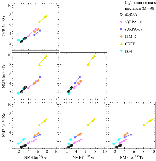
Figure 2: NMEs of several elements in different models for the light neutrino mass mechanism.

Figure 3: NMEs of several elements in different models for the heavy neutrino mass mechanism.

To get a general idea of errors brought by different approaches, we start from a common case mentioned above with CD-Bonn src and bare $g_{A}$. We find from these tables that for most nuclei, the ISM sets the lower bound of the results for the light mass mechanism while IBM-2 sets the lower bound for the heavy mass mechanism. While for the upper bound, CDFT always has the largest values for the light neutrino mass mechanism, sQRPA gives the upper bound for most nuclei with the heavy neutrino mass mechanism. At the light neutrino mass end, our dQRPA calculation can be even smaller than the ISM results for semi-magic ¹³⁶Xe. This may come from the number non-conservation nature of QRPA methods (for sQRPA, the overlap factor between the parent and daughter nuclei is not included, therefore this effect will not appear). It is found that the restoration of particle number conservation will enhance the NMEs for semi-magic nuclei as from the DFT calculations Yao:2014uta . While for light neutrino mass mechanism, model space dependence is not important, the heavy neutrino mass case, the NME is closely related to model space Brown:2015gsa . This explains why the dQRPA and ISM give similar results at one end and ISM gives much smaller results at the other end. Alternatively, the major difference between QRPA and CDFT is the inclusion of so-called iso-scalar pairing. This correlation is supposed to be responsible for the suppression of NMEs of both $2\nu\beta\beta$ and $0\nu\beta\beta$ processes Hinohara:2014lqa . But one also finds that this sensitivity applies only for light neutrino mass mechanism and the heavy neutrino mass mechanism depends less on this correlation Fang:2018tui . This also explains the large discrepancy for CDFT and QRPA at one end but their similarity at another end. Except for ¹³⁶Xe, for microscopic models, the general trend is at light neutrino mass mechanism case, ISM with more many-body correlations may be more close to the actual NME but for heavy neutrino mass mechanism, models with large model space may be more reliable. In this sense, dQRPA calculations which agree with ISM for light neutrino mass mechanism and with CDFT for heavy neutrino mass mechanism appear to be reliable, although a careful model benchmark is needed before a concrete conclusion. In general, the discrepancies from various methods can be explained qualitatively Agostini:2022zub , but quantitative calculations need to be performed to pin down the deviations as have done in Brown:2015gsa .

These analyses are well illustrated by Fig. 2 the light neutrino mass mechanism case and Fig. 3 the heavy neutrino mass mechanism case as well as in Fig. 1 for the whole neutrino mass region. Due to the availability of calculated results, the different color bands for different methods are not equal-footing. For all QRPA methods, we have results for both quenched and bare case of $g_{A}$, but for IBM-2 and CDFT, only results of the bare case $g_{A}$ are available. As we stated above, the two external sources for uncertainty commonly discussed which is model independent are the values of $g_{A}$ and the corrections from short range behaviour of nuclear force. A naive estimation of the possible errors from $g_{A}$ is about certain given that $M_{F}\lesssim 1/3M_{GT}$ and $M_{T}$ is small. Under such assumptions, a choice of $g_{A}$ around 0.75 gives an uncertainty of about 20% or less. While for light neutrino mass mechanism, except the wilder Miller-Spencer src, modern src gives a correction of about 5%$\sim$10% to the NME. Therefore for light neutrino case, the quenching may be important for the uncertainty estimation. While for the heavy neutrino mass case, the neutrino potential behaves like a contact potential. Therefore the short-range behaviour of nucleons becomes much more important. For milder CD-Bonn src, a 20%$\sim$30% reduction is expected and this reduction could be enhanced to 30%$\sim$50% for Argonne src and more than 50% for Miller-Spencer src. Even without the wildest Miller-Spencer src, the uncertainty brought by src is the most significant source for errors for heavy neutrino mass. In general, the errors from these external sources are quantifiable. That is, the errors are in general 20% at light neutrino end and a modest estimation with inclusions of more modern src will restrict the errors at heavy neutrino end by 50%. The errors for arbitrary neutrino mass therefore lie in between 20% to 50% if quenching and srcs are considered.

3 Numerical Results

3.1 The parameter space of effective neutrino mass revisited

As shown in Eq. (18), the effective neutrino mass $m_{\rm eff}$ depends on five parameters, $m_{\rm eff}^{\nu}$, $M_{1}$, $M_{2}$, $|R_{e1}^{2}|$ and $\delta_{14}$. In Ref. Fang:2021jfv , the authors have studied how the involvement of right-handed neutrinos can magnify or decrease the magnitude of effective neutrino mass. We revisit the parameter space of $m_{\rm eff}$ in more details. Considering $3\sigma$ ranges from the current global fit of neutrino oscillation data and allowing the Majorana phases $\alpha_{2}$ and $\alpha_{3}$ changing from $0$ to $2\pi$, we have $0.96~{}{\rm meV}\leq m_{\rm eff}^{\nu}\leq 4.2~{}{\rm meV}$ for NMO and $14.7~{}{\rm meV}\leq m_{\rm eff}^{\nu}\leq 49.2~{}{\rm meV}$ for IMO. The whole IMO range will be explored by the next-generation $0\nu\beta\beta$ experiments while the NMO range needs more ambitious proposals beyond. Having the mixed contribution from the heavy neutrino parameters $(M_{1},M_{2},|R_{e1}^{2}|,$ and $\delta_{14})$, it’s difficult to discriminate the neutrino mass orderings from $0\nu\beta\beta$ experiments. Assuming a fixed value of $m_{\rm eff}^{\nu}$, the $m_{\rm eff}$ can be as small as 0 or exceed the current experimental limit depending on the heavy neutrino parameters. In Figs. 5 and 6, we take the NME interpolation formula in Eq. (15) and illustrate the contour plot of $m_{\rm eff}$ by typically taking $\delta_{14}=0$ or $\pi/2$, $\alpha_{2}-\alpha_{3}=0$ for NMO, $\alpha_{2}=0$ for IMO, the NME values in the dQRPA model with $g_{A}=1$ and Argonne src, as well as the best-fit values of related neutrino oscillation parameters Esteban:2020cvm . Some comments are as follows:

• The dependence of $m_{\rm eff}$ on the heavy neutrino parameters in the NMO or IMO case can be very different because the NMO range of $m_{\rm eff}^{\nu}$ is about one order smaller than its IMO range. The yellow region and orange region correspond to the NMO range and the IMO range, respectively. While the current $0\nu\beta\beta$ experiments already reach part of the IMO range assuming big end of NME value, the next-generation proposals will detect the whole IMO range space and beyond. Given some upper limit of $m_{\rm eff}$ from experiments, bigger parameter space will be usually excluded in the IMO case.

• Same as Ref. Fang:2021jfv , $\delta_{14}=0$ or $\pi/2$ are taken as typical examples. According to Eq. (18) and as shown in Figs. 5 and 6, in the case of $M_{1}>M_{2}$, $m_{\rm eff}$ with $\delta_{14}=0$ is smaller than its value with $\delta_{14}=\pi/2$ and the conclusion is opposite in the case of $M_{1}<M_{2}$.

• In the limit of $M_{1}=M_{2}$, we have $m_{\rm eff}=|m_{\rm eff}^{\nu}[1-f_{\beta}(M_{2})]|$ Fang:2021jfv . $f_{\beta}(M_{2})$ depend on both $M_{2}$ and $<p^{2}>=m_{p}m_{e}(M_{\rm H}/M_{L})$, where $\sqrt{<p^{2}>}$ varies from 62.5 MeV to 249.0 MeV from Tables 1 and 2. $m_{\rm eff}$ may take any value from 0 to $m_{\rm eff}^{\nu}$ depending on the input of $M_{2}$. We display how $f_{\beta}(M_{N})$ and $m_{\rm eff}$ in the limit $M_{1}=M_{2}$ change with heavy neutrino mass in Fig. 4, where the bands are due to the uncertainties from $m_{\rm eff}^{\nu}$. With $M_{1}=M_{2}$ as a boundary, the $M_{\rm eff}$ depends on $M_{1}$, $M_{2}$ and $|R_{e1}^{2}|$ very differently especially with bigger $|R_{e1}^{2}|$, which leads to the peak shape in Fig. 5 and the asymmetric feature about the diagonal $M_{1}=M_{2}$ line.

• If $m_{\rm eff}$ is big enough, as the $m_{\rm eff}$ increases, the contribution of $m_{\rm eff}^{\nu}$ decreases due to the small ranges of $m_{\rm eff}^{\nu}$ values. In the dark red region, the effects of $m_{\rm eff}^{\nu}$ is negligible. One can refer to Fang:2021jfv for more discussion of the contribution of $m_{\rm eff}^{\nu}$.

• From Fig. 6, the contours of big $m_{\rm eff}$ only appears in the part of $M_{1}>M_{2}$ when $|R_{e1}^{2}|$ is small enough while with $|R_{e1}^{2}|$ being big enough, the contours of $m_{\rm eff}$ consist of two parts, one in the case of $M_{1}>M_{2}$, the other $M_{1}<M_{2}$. $m_{\rm eff}$ in the lower left corner and upper right corners is always not very big, especially for the NMO case. For the former, it is because $f_{\beta}(M_{N})$ is not far away from 1, leading to $m_{\rm eff}^{\nu}$ suppressed and meanwhile $M_{1}$ is not big enough or very different from $M_{2}$. For the latter, the smallness of $m_{\rm eff}$ is mainly because the two heavy neutrino masses are not different enough, where the contribution $m_{\rm eff}^{\nu}$ dominates.

• With both $M_{1}$ and $M_{2}$ being small enough as well as $M_{1}\neq M_{2}$, $m_{\rm eff}$ can be very small, which is far beyond the exploration reach of next-generation $0\nu\beta\beta$ experiments. While when $|R_{e1}^{2}|$ is big enough and $M_{1}$ is much bigger than $M_{2}$, $m_{\rm eff}$ is very big and excluded by current experiments (such as the lower part of the dark red region in 6).

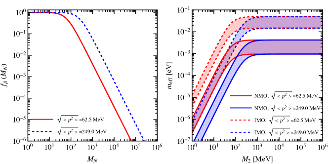
Figure 4: Left panel: the illustration of how $f_{\beta}(M_{N})$ changes with $M_{N}$; right panel: $m_{\rm eff}$ changing with $M_{2}$ in the limit $M_{1}=M_{2}$. In both figures, the interpolation formula in Eq. (15) and two specific values of $\sqrt{<p^{2}>}$ are used.

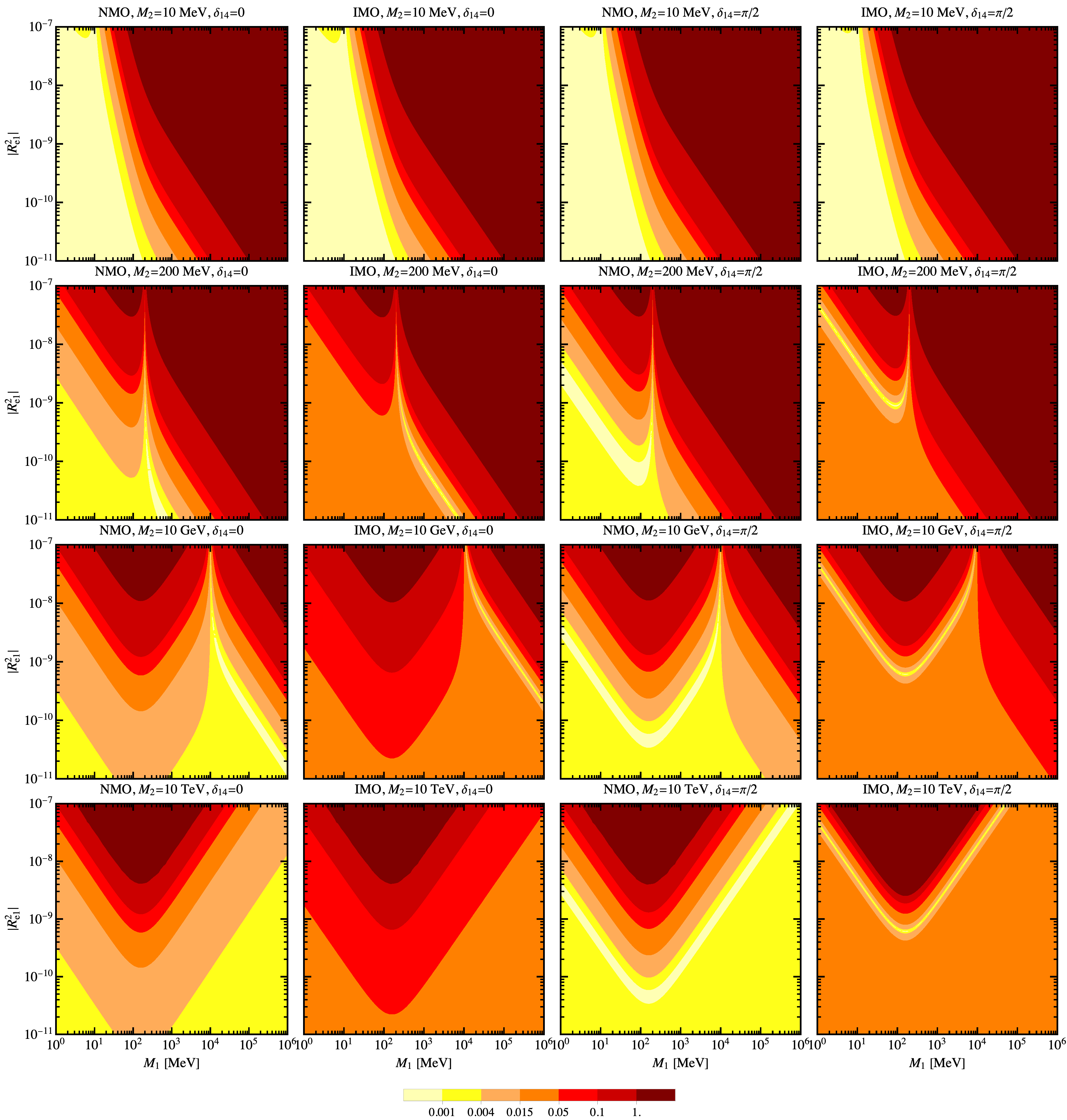
Figure 5: The contour plot of $m_{\rm eff}$ in the dimensions of $M_{1}$ and $|R_{e1}^{2}|$ by typically taking $\delta_{14}=0$ or $\pi/2$, $\alpha_{2}-\alpha_{3}=0$ for NMO, $\alpha_{2}=0$ for IMO, the NME values in the dQRPA model with $g_{A}=1$ and Argonne src, as well as the best-fit values of related neutrino oscillation parameters Esteban:2020cvm , where the $m_{\rm eff}$ values in the legend are in unit of eV.

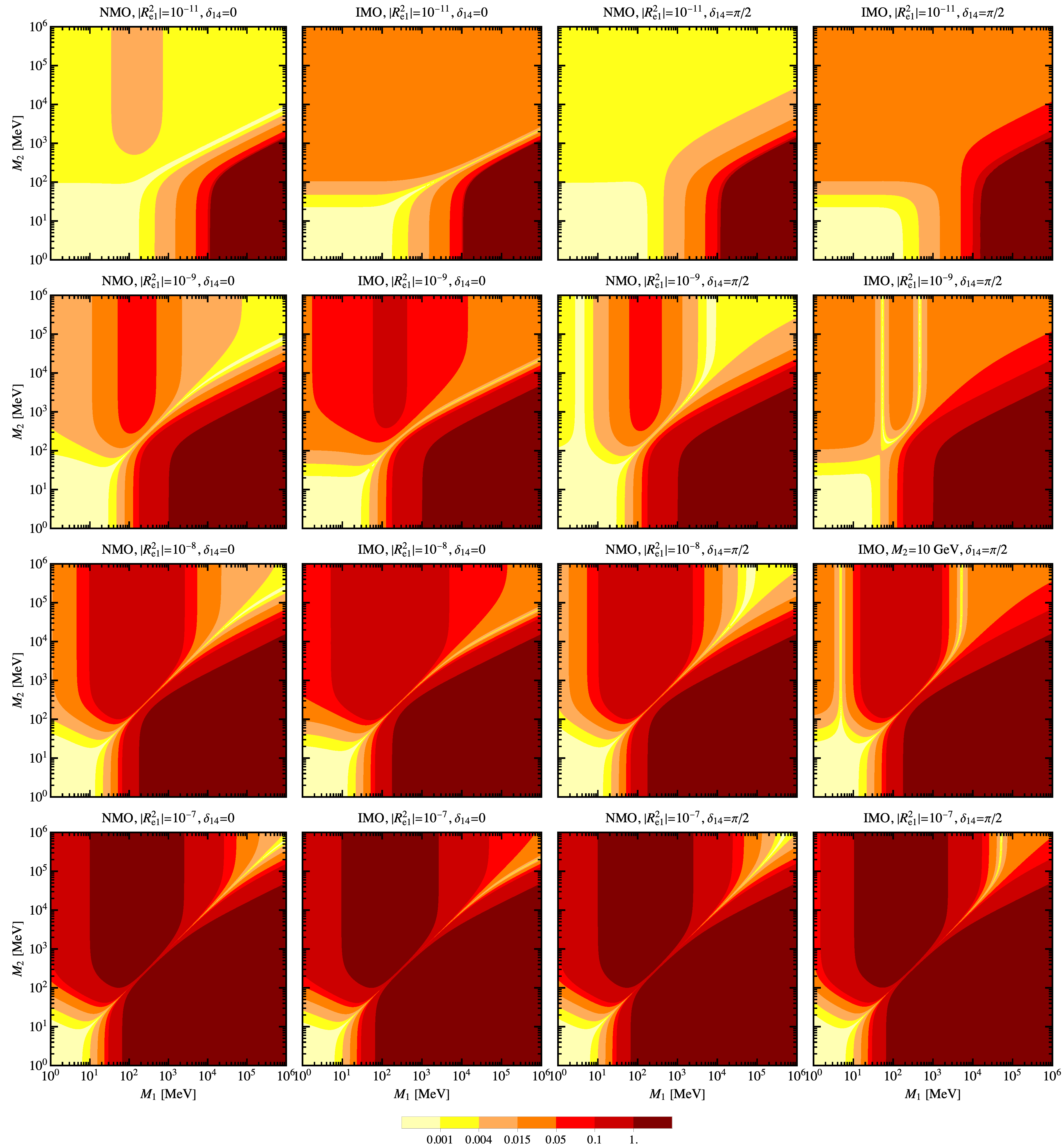
Figure 6: The contour plot of $m_{\rm eff}$ in the dimensions of $M_{1}$ and $M_{2}$ by typically taking $\delta_{14}=0$ or $\pi/2$, $\alpha_{2}-\alpha_{3}=0$ for NMO, $\alpha_{2}=0$ for IMO, the NME values in the dQRPA model with $g_{A}=1$ and Argonne src, as well as the best-fit values of related neutrino oscillation parameters Esteban:2020cvm , where the $m_{\rm eff}$ values in the legend are in unit of eV.

3.2 Constraints from current neutrinoless double beta decay experiments

More specifically, let us interpret the current $0\nu\beta\beta$ experiment data in the framework of minimal type-I seesaw model. We mainly focus on the upper limit of the effective neutrino mass $m_{\rm eff}$ and the constraints on heavy neutrino parameters by reasonably combining the current available $0\nu\beta\beta$ data. According to Eq. (17) and the definition of $m_{\rm eff}$ in Eq. (18), the upper limit of $m_{\rm eff}$ in the framework of minimal type-I seesaw is equal to the upper limit of $m_{\rm eff}^{\nu}$ in the light-neutrino exchange mechanism. We use the terminology of the $m_{\rm eff}$ upper limit below. Currently, the strongest constraints of $0\nu\beta\beta$ are obtained from GERDA GERDA:2020xhi , MAJORANA Majorana:2022udl CUORE CUORE:2021mvw , KamLAND-Zen KamLAND-Zen:2022tow , and EXO-200 EXO-200:2019rkq experiments. Most experimental papers provide only the lower limits of $T^{0\nu}_{1/2}$ at 90% C.L. instead of its $\Delta\chi^{2}$ function while the $\Delta\chi^{2}$ values of KamLAND-Zen and CUORE experiments are directly given by the experiment collaborations in Refs. CUORE:2021mvw ; KamLAND-Zen:2022tow . We construct approximately the $\Delta\chi^{2}$ functions of GERDA, MAJORANA and CUORE similar to Refs. Caldwell:2017mqu ; Biller:2021bqx ; Capozzi:2021fjo ; Lisi:2022nka ; Pompa:2023jxc ; Lisi:2023amm by parameterizing $\Delta\chi^{2}(1/T_{1/2}^{0\nu})$ as:

$$\Delta\chi^{2}_{r}(1/T_{1/2}^{0\nu})=a_{r}(1/T_{1/2}^{0\nu})^{2}+b_{r}(1/T_{1/2}^{0\nu})+c_{r}\;,$$ (20)

where $T^{0\nu}_{1/2}$ is in unit of $10^{25}~{}\mathrm{yr}$ and the subscript $r$ ($r=$ GERDA, MAJORANA, CUORE, KamLAND-Zen and EX0-200) label different experiments. Note that for KamLAND-Zen experiment, with $\Delta\chi^{2}$ values only for small $T_{1/2}^{0\nu}$ KamLAND-Zen:2022tow , we fit them according to Eq. (20) to get $\Delta\chi^{2}_{r}(1/T_{1/2}^{0\nu})$. As for the CUORE experiment, we fit the available $\Delta\chi^{2}_{r}(1/T_{1/2}^{0\nu})$ curve given by CUORE:2021mvw in accordance with Eq. (20) for the convenience of later calculations.

Table 3 shows the derived values of $a_{r}$, $b_{r}$ and $c_{r}$ as well as the corresponding 90% C.L. ($\Delta\chi^{2}=2.706$) half-life limits compared with the results published in the experiment papers . We can see the limits obtained from the $\Delta\chi^{2}$ function following Eq. (20) agree well with the published results. The $\Delta\chi^{2}(1/T^{0\nu}_{1/2})$ functions are displayed in Fig. 7, where we know the most stringent upper limit of $0\nu\beta\beta$ half life is of order $10^{25}$ or $10^{26}$ year at 90% C.L. dependent of the relevant isotope.

Experiment	Isotope	$a_{r}$	$b_{r}$	$c_{r}$	$T^{0\nu}_{1/2}/10^{25}$yr (90%C.L.)	expt. (90%C.L.)	Reference
GERDA	${}^{76}\mathrm{Ge}$	$0.000$	48.708	0.000	18.0	18	GERDA:2020xhi
MAJORANA	${}^{76}\mathrm{Ge}$	$0.000$	22.460	0.000	8.30	8.3	Majorana:2022udl
CUORE	${}^{130}\mathrm{Te}$	$44.300$	$-3.417$	0.066	2.61	2.6	CUORE:2021mvw
KamLAND-Zen	${}^{136}\mathrm{Xe}$	$527.773$	38.780	0.000	22.86	23	KamLAND-Zen:2022tow
EXO-200	${}^{136}\mathrm{Xe}$	$56.041$	$-18.325$	1.511	3.50	3.5	EXO-200:2019rkq

Table 3: The coefficients of approximate $\Delta\chi^{2}(1/T^{0\nu}_{1/2})$ functions as well as the corresponding 90% C.L. half-life limits, compared with the publication by the experiment collaborations.

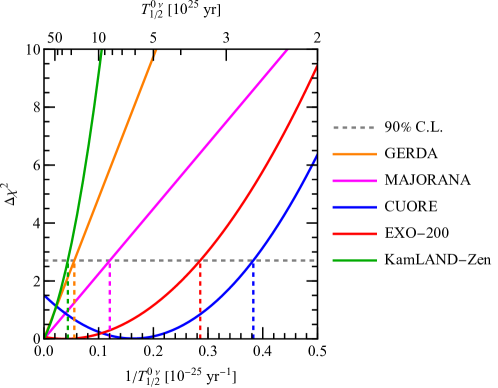
Figure 7: $\Delta\chi^{2}$ for the various experiments as function of $1/T^{0\nu}_{1/2}$ and $T^{0\nu}_{1/2}$.

In order to fully interpret the existing $0\nu\beta\beta$ results, even though we can not combine all the experiments in Table 3 to give a valid half life because the isotope of each experiment is not always the same, we can combine these experimental results to constrain the common part such as the effective neutrino mass $m_{\rm eff}$ and other new-physics parameters involved in $m_{\rm eff}$. Since these experiments are independent observations, the combined $\Delta\chi^{2}$ function for $(T^{0\nu}_{1/2})^{-1}$ is parameterized as summing individual $\Delta\chi^{2}_{r}$ function of all $0\nu\beta\beta$ experiments,

$$\chi^{2}_{0\nu\beta\beta}= \Delta\chi^{2}_{\mathrm{GERDA}}[(T^{0\nu,^{76}\mathrm{Ge}}_{1/2})^{-1}]+\Delta\chi^{2}_{\mathrm{MAJORANA}}[(T^{0\nu,^{76}\mathrm{Ge}}_{1/2})^{-1}]\;,\Delta\chi^{2}_{\mathrm{CUORE}}[(T^{0\nu,^{130}\mathrm{Te}}_{1/2})^{-1}]$$ (21)

$$+\Delta\chi^{2}_{\mathrm{KamLAND-Zen}}[(T^{0\nu,^{136}\mathrm{Xe}}_{1/2})^{-1}]+\Delta\chi^{2}_{\mathrm{EXO-200}}[(T^{0\nu,^{136}\mathrm{Xe}}_{1/2})^{-1}]\;,$$

where $T^{0\nu,^{130}\mathrm{Te}}_{1/2}$, $T^{0\nu,^{136}\mathrm{Xe}}_{1/2}$ and $T^{0\nu,^{76}\mathrm{Ge}}_{1/2}$ are the half-life of the ${}^{130}\mathrm{Te}$, ${}^{136}\mathrm{Xe}$ and ${}^{76}\mathrm{Ge}$, respectively, and can be determined by inputting NME, phase space factor and $m_{\mathrm{eff}}$ as in Eq. (17).

From Eq. (17), the NMEs will make an effect of the relationship of the $m_{\mathrm{eff}}$ ($m_{\mathrm{eff}}^{\nu}$) and the $T^{0\nu}_{1/2}$, and the values of NMEs are very different in various models, which contribute the dominated uncertainty to the constraints of the $T^{0\nu}_{1/2}$ as well as $m_{\mathrm{eff}}$. Typically, Fig. 8 shows the $\Delta\chi^{2}$ as a function of $m_{\mathrm{eff}}$ in dQRPA model with $g_{A}=1$ and Argonne src. We can see that the constraint of $m_{\mathrm{eff}}$ from GERDA is the most stringent, the constraint from KamLAND-Zen is competitive with that from GERDA, and constraint from EXO-200 is the weakest, although the constraint of $T^{0\nu}_{1/2}$ from EXO-200 is more stringent than CUORE, due to the different NME values and the phase spaces of different isotopes.

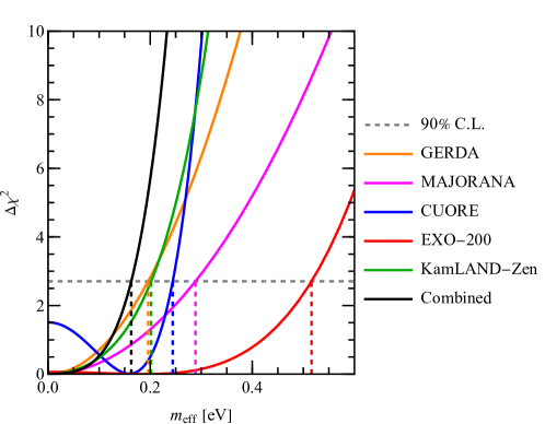
Figure 8: $\Delta\chi^{2}$ of the $m_{\mathrm{eff}}$ in dQRPA model ($g_{A}=1$ and Argonne src) for the various experiments.

Note that the combined results are derived from $\chi^{2}_{0\nu\beta\beta}$ by subtracting its minimum value regarding $m_{\rm eff}$. More generally, we consider various NME models we discussed in last section. In this case, things will be different due to the different prediction of the NMEs from different nuclear models. Fig. 9 shows the 90% C.L. limits of $m_{\mathrm{eff}}$ for various experiments obtained by different nuclear models, and the results of combined analysis from $\chi^{2}_{0\nu\beta\beta}$ are also shown on the right side of the figure. The different markers stand for the different nuclear models. The gray region represents the IMO range of $m_{\rm eff}^{\nu}$. From Fig. 9, the dQRPA model will always get a weak limit, while the CDFT models will always get a strengthened limits due to their larger values for predicted NMEs. We can regard the different NME calculation as a global NME uncertainty, and it will result in an order of magnitude uncertainty for the constraints on $m_{\mathrm{eff}}$. The most stringent limits are obtained from KamLAND-Zen experiment, and in the CDFT model, these constraints already exclude part of IMO region given the light neutrino exchange mechanism. We can also find that the combined analysis of all the experiments will strength the constraints of $m_{\mathrm{eff}}$, but considering the NME uncertainty, it is still far away to reject IMO case.

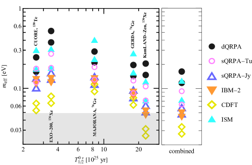
Figure 9: 90% C.L. upper bounds of the $m_{\mathrm{eff}}$ for the various experiments.

The constraints of various experiments can be also shown in Fig. 10, and the relation between the $T^{0\nu}_{1/2}$ of ${}^{76}\mathrm{Ge}$, ${}^{130}\mathrm{Te}$ and ${}^{136}\mathrm{Xe}$ for different NME calculations is also shown. The different markers stand for the different $m_{\rm eff}$ values. According to Eq. (17), the half-lives between two different isotopes are linearly correlated on a logarithmic scale and the position of line is determined by the ratio of the phase spaces and the NME model. For a certain pair of elements, the ratio of their phase spaces is a constant, so the slope of the line is determined by the ratio of NMEs. In the pair of ${}^{76}\mathrm{Ge}$ and ${}^{136}\mathrm{Xe}$, the line of dQRPA is the uppermost line and the line of CDFT is in the bottom, which means that if the half-life of ${}^{76}\mathrm{Ge}$ is determined, the prediction of the half-life of ${}^{136}\mathrm{Xe}$ is longest in dQRPA calculation, and shortest in CDFT calculation. Considering the pair of ${}^{76}\mathrm{Ge}$ and ${}^{130}\mathrm{Te}$, when the half-life of ${}^{76}\mathrm{Ge}$ is determined, the half-life of ${}^{130}\mathrm{Te}$ is longer in sQRPA and IBM-2 calculation, and still shortest in CDFT calculation. As for the pair of ${}^{130}\mathrm{Te}$ and ${}^{136}\mathrm{Xe}$, when the half-life of ${}^{130}\mathrm{Te}$ is determined, the half-life of ${}^{136}\mathrm{Xe}$ is longest in dQRPA calculation, and shortest in ISM calculation. It is also easy to see that the relationship of the half-life between different elements in one NME model is almost independent of the assumption in this model, i.e. $g_{A}$ and srcs, although the half-life is different based on some certain value of $(m_{\mathrm{eff}})^{2}$ by different assumptions of the same NME model.

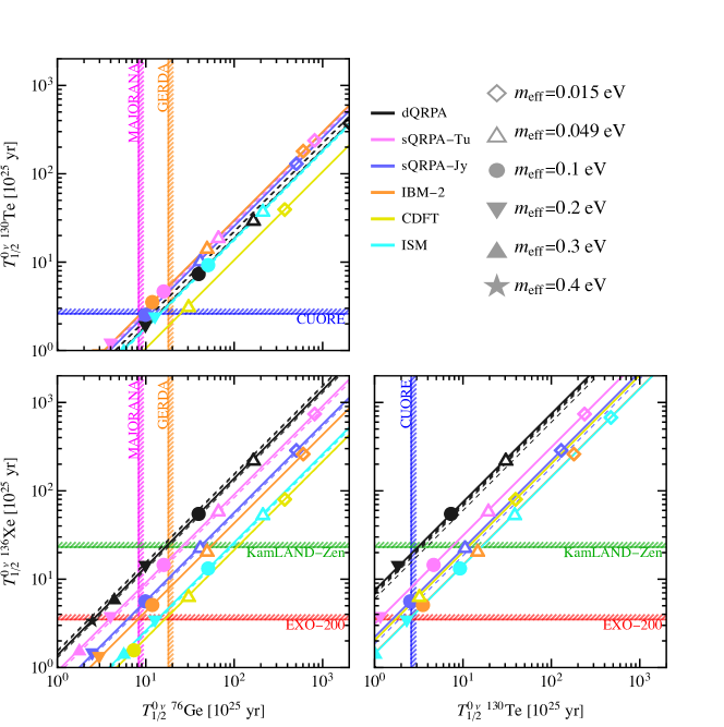
Figure 10: Relation between the $T^{0\nu}_{1/2}$ in ⁷⁶Ge, ¹³⁶Xe and ¹³⁰Te for different matrix element calculations.

According to Fig. 9, we can roughly get the corresponding constraints on the heavy neutrino parameters in the case of dQRPA model ($g_{A}=1$, Argonne src) from Figs. 5 and 6 (mainly the red regions). Next we will discuss the constraints on the minimal Type-I seesaw model depending on the NME models in more details. In the SM, the 0$\nu\beta\beta$ decay experiments will constrain the three active neutrinos. And in the seesaw model, the RHNs will directly contribute to the $m_{\mathrm{eff}}$ of the 0$\nu\beta\beta$ decay, so the 0$\nu\beta\beta$ decay experiments constrain RHNs and three active neutrinos together. The intrinsic relation in the seesaw mechanism leads to that only 4 free parameters of RHNs exist, and for convenience, we choose two masses of RHNs $M_{1}$, $M_{2}$, the absolute value of $R_{e1}^{2}$, and the mixing phase $\delta_{14}$. The contribution of the active neutrino part from $m_{\rm eff}^{\nu}$ can be constrained by the neutrino oscillation measurement, cosmological observation, and $\beta$-decay experiments, but in the minimal Type-I seesaw model we considered in this work, the lightest neutrino mass is assumed to be zero, so only the oscillation measurement is relevant and considered in the analysis. To extract information involved in $m_{\rm eff}$, the final $\chi^{2}_{\rm tot}$ function is defined as

$$\chi^{2}_{\rm tot} =\chi^{2}_{0\nu\beta\beta}+\chi^{2}_{\mathrm{OSC}}\;,$$ (22)

Here

$$\chi^{2}_{\mathrm{OSC}}=\sum_{i}\frac{(\eta_{i}-\eta_{i}^{\rm BF})^{2}}{\sigma_{i}^{2}};,$$ (23)

where $\eta_{i}$ denote in turn the oscillation parameters $\{\theta_{12},~{}\theta_{13},~{}\Delta m_{21}^{2},~{}\Delta m_{31}^{2}\}$ with $\Delta m_{ij}^{2}\equiv m_{i}^{2}-m_{j}^{2}$ (for $ij=21,~{}31$), and $\eta_{i}^{\rm BF}$ and $\sigma_{i}$ stand for the best-fit values and symmetrized $1\sigma$ errors of $\eta_{i}$, respectively.

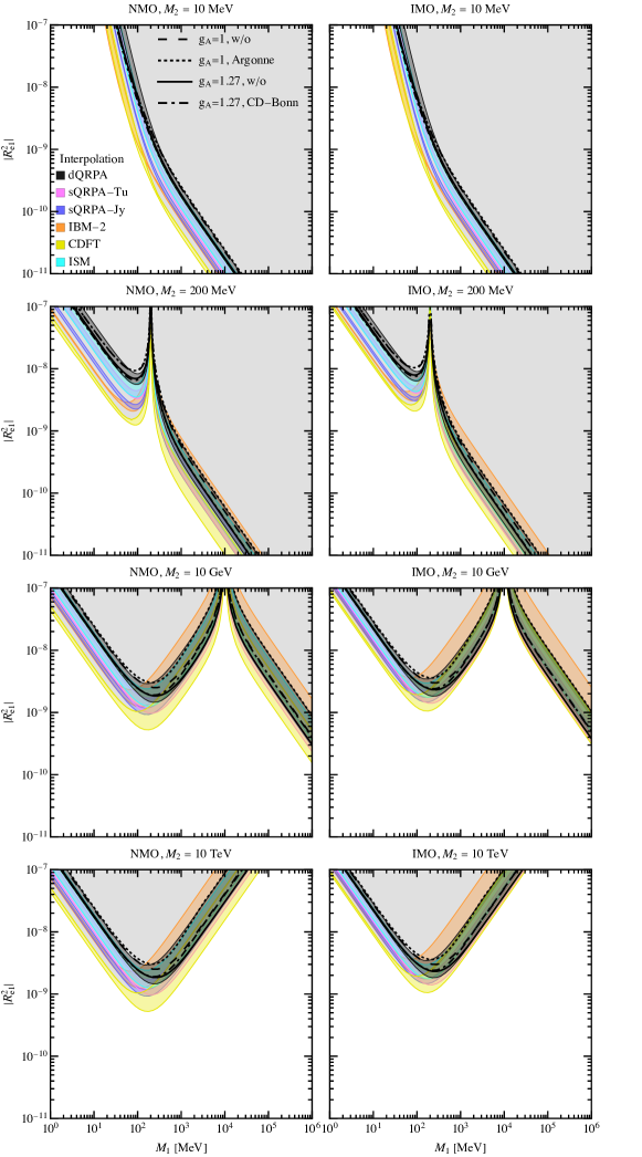
Figure 11: Excluded regions of the $M_{1}$ and $|R^{2}_{\mathrm{e1}}|$ given fixed $M_{2}$ in the case of different NME models by combining current results from GERDA, MAJORANA, CUORE, KamLAND-Zen, and EXO-200 experiments.

In Fig. 11, we present the $3\sigma$ constraints of $M_{1}$ and $|R_{e1}^{2}|$ with the fixed values of $M_{2}=10~{}\mathrm{MeV},200~{}\mathrm{MeV},10~{}\mathrm{GeV}$, $10~{}\mathrm{TeV}$. The way is to first calculate the minima of $\chi^{2}_{\rm tot}$ by scanning the neutrino oscillation parameters in their $3\sigma$ ranges, Majorana phases in $[0,2\pi]$, and $\delta_{14}$ in $[0,\pi]$ for fixed values of $M_{1}$, $|R_{e1}^{2}|$ and $M_{2}$. Then the $3\sigma$ constraints correspond to the contour $(\chi^{2}_{\rm tot})_{\rm min}\simeq 11.83$ for two degrees of freedom. Similarly, we present the $3\sigma$ constraints of $M_{1}$ and $M_{2}$ with the fixed values of $|R_{e1}^{2}|=10^{-11},10^{-9},10^{-8},10^{-7}$ in Fig. 12. Some discussions about these two figures are as follows.

• The NMO and IMO cases are similar while the former case will exclude a little more parameter space than the latter one. This is implied in Figs. 5 and 6 when $m_{\rm eff}$ is not very small, for example the light-red region in the case of $\delta_{14}=\pi/2$ (namely, the three and four columns).

• The gray regions represent the $3\sigma$ excluded regions derived from current experiments in the case of CDFT model. The colorful boundary bands display the differences of NME models. The NME models can induce about one order uncertainties on the constraints of $M_{1}$, $M_{2}$ and $|R_{e1}^{2}|$ as shown in Figs. 11 and 12.

• The IBM-2 model can exclude more parameter space of RHNs, while the dQRPA model will exclude less parameter space of RHNs. When $M_{1}$ is smaller than $200~{}\mathrm{MeV}$. The reason is that the prediction of NMEs in light neutrino mass in the dQRPA model is smaller than the IBM-2 model, and in heavy neutrino mass the reverse applies. For the similar reason, when $M_{1}$ is larger than $200~{}\mathrm{MeV}$, the case of ISM model is competitive with the dQRPA model.

• The hierarchy of constraints changes at different $M_{2}$, since the hierarchy of the NMEs changes at different mass of RHNs. The variation of the upper bounds is small when $M_{2}$ is small, and is large when $M_{2}$ is large, especially in the case that $M_{1}$ is also large. The variation in CDFT is the largest one, and the constraints in dQRPA and ISM models have the smallest variation.

• In the case of $M_{2}$ around $10~{}\mathrm{TeV}$, the constraints on two RHNs are similar to the case of one generation RHN. The combined analysis in this case will constrain $|R_{e1}^{2}|<10^{-8}\sim 10^{-9}$ when $M_{1}$ is around $200~{}\mathrm{MeV}$, and $|R_{e1}^{2}|<10^{-8}\sim 10^{-7}$ when $M_{1}$ is around $1~{}\mathrm{MeV}$. In the case of small $M_{2}$, the combined analysis will exclude the large $M_{1}$ region, and with the $|R_{e1}^{2}|$ decreasing, the allowed region of $M_{1}$ is expanded.

• In the case of $M_{2}$ is around $200~{}\mathrm{MeV}$ or $10~{}{\rm GeV}$, there is a peak also around $200~{}\mathrm{MeV}$ or $10~{}{\rm GeV}$. The constraints of $|R_{e1}^{2}|$ are much weaker compared with the constraints when $M_{1}$ deviated enough from $200~{}\mathrm{MeV}$ or $10~{}{\rm GeV}$. This is due to the degeneracy of two RHN masses, where the $m_{\rm eff}$ is not sensitive to $|R_{e1}^{2}|$ from Eq. (18).

• From Fig. 12 showing the $3\sigma$ excluded regions of $M_{1}$ and $M_{2}$ given fixed $|R_{e1}^{2}|$, it’s obvious that as $|R_{e1}^{2}|$ is bigger, more parameter space of $M_{1}$ and $M_{2}$ will be excluded. With $|R_{e1}^{2}|$ being very small, only the right corner can be excluded. In the case of $|R_{e1}^{2}|=10^{-9}$, the excluded regions for dQRPA, IBM-2 and ISM models consist only one part in the half plane of $M_{1}>M_{2}$. This is due to relatively small NME values leading to smaller upper limit of $m_{\rm eff}$ compared with sQRPA-Tu, sQRPA-Jy and CDFT models.

• In the lower two panels with $|R_{e1}^{2}|=10^{-8}$ and $|R_{e1}^{2}|=10^{-7}$ of Fig. 12, a big parameter space of $M_{1}$ and $M_{2}$ is excluded while the diagonal line $M_{1}=M_{2}$ still survives due to the small values of $m_{\rm eff}$ in this case. When both $M_{1}$ and $|R_{e1}^{2}|$ are small enough, $M_{2}$ is allowed in whole mass range. This is because the third term in $m_{\rm eff}$, which is $|R_{e1}^{2}|e^{2{\rm i}\delta_{14}}M_{1}[f_{\beta}(M_{1})-f_{\beta}(M_{2})]$, is suppressed according to Eq. (18). While in the case of $|R_{e1}^{2}|=10^{-7}$, only the lower left corner with small $M_{1}$ and $M_{2}$ and the upper right corner with big $M_{1}$ and $M_{2}$ are allowed, where the heavy neutrino mass mechanism and light neutrino mass mechanism dominate, respectively.

Other experiments have also studied the properties and limitations of right-handed neutrinos, in addition to neutrinoless double beta decay experiments. Cosmological observations, data from large hadron colliders, the neutrino probe T2K:2019jwa ; MicroBooNE:2019izn ; MicroBooNE:2019izn and charged lepton flavor violation search Lindner:2016bgg provide important information about the mass and interactions of right-handed neutrinos. However, these results are often derived under the assumption of a single right-handed neutrino mixing with a single flavor, which may not be applicable in realistic seesaw models. The constraints on the mixing $|R^{2}_{e1}|$ from the colliders is the level of [$10^{-8}$, $10^{-9}$] by NA62 NA62:2020mcv for $150\;{\rm MeV}<M_{1}<400\;{\rm MeV}$, and [$10^{-6}$, $10^{-7}$] by CHARM CHARM:1985nku for $400\;{\rm MeV}<M_{1}<2\;{\rm GeV}$, and the level of $10^{-4}$ for $M_{1}>2\;{\rm GeV}$ by Belle Belle:2013ytx , DELPHI DELPHI:1996qcc , ATLAS ATLAS:2019kpx and CMS CMS:2018iaf . The results from the neutrino probe, T2K T2K:2019jwa , suggest the limit $|R^{2}_{e1}|$ varies from $10^{-7}$ to $10^{-9}$ for the mass range of $150\;{\rm MeV}<M_{1}<500\;{\rm MeV}$. The case under the assumption of a single right-handed neutrino mixing with a single flavor is similar to the case of the one RHNs mass large enough, compared with the results of this work. We have showed that in this case, the $0\nu\beta\beta$ experiment remains the strongest constraint on RHNs, particularly for heavier masses, as discussed in Ref. Faessler:2014kka . Although the constraints on the mixing matrix from the $0\nu\beta\beta$ experiment are weaker for lower masses, this range is not covered by other experiments. For masses around 1 GeV, the $0\nu\beta\beta$ experiment provides the strongest constraints on the mixing matrix elements, while other experiments provide similar or even better constraints, so that the results from these experiments can complement each other in this case.

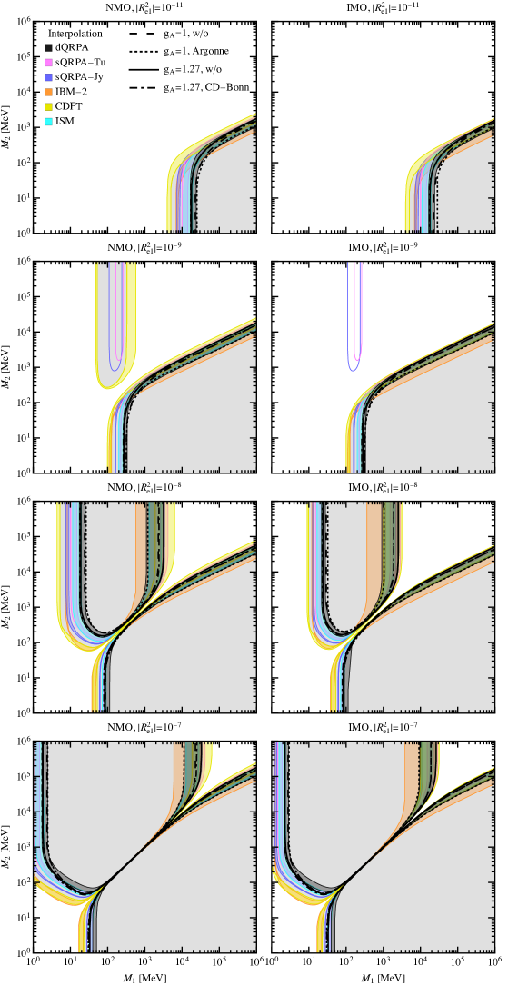
Figure 12: Excluded regions of the $M_{1}$ and $M_{2}$ given fixed $|R_{e1}^{2}|$ in the case of different NME models by combining current results from GERDA, MAJORANA, CUORE, KamLAND-Zen, and EXO-200 experiments.

3.3 Sensitivities of future experiments

For the sensitivities of future $0\nu\beta\beta$ experiments, we refer to the analysis scheme in Ref. Pompa:2023jxc and use the $\chi^{2}$ function based on the Poisson distribution

$$\Delta\chi_{ij}^{2}(m_{\rm eff},(M_{0\nu})_{\alpha j};m_{\rm eff}^{\rm True},(M_{0\nu})_{\alpha i}^{\rm True})=2\sum_{\alpha}(N_{\alpha j}-N_{\alpha i}^{\rm True}+N_{\alpha i}^{\rm True}{\rm In}\frac{N_{\alpha i}^{\rm True}}{N_{\alpha j}})\;,$$ (24)

where the subscript $\alpha$ denotes different isotopes/experiments and $i,j$ stand for different NME models. $N_{\alpha i}^{\rm True}=B_{\alpha i}+S_{\alpha i}(m_{\rm eff}^{\rm True},(M_{0\nu})_{\alpha i}^{\rm True})$ is the total event number expected from a given experiment and some true NME value and true $m_{\rm eff}$ chosen by the Nature, and $N_{\alpha j}=B_{\alpha j}+S_{\alpha j}(m_{\rm eff},M_{\alpha j})$ represents the model to be compared with the “true” one. Note that the NME $M_{\alpha j}$ and $M_{\alpha i}^{\rm True}$ depend on neutrino mass, which differs from Ref. Pompa:2023jxc . $S_{\alpha i}$ and $B_{\alpha i}$ are the expected numbers of signal and background events, respectively. They can be derived from $S_{\alpha i}(m_{\rm eff},~{}M_{\alpha i})={\rm In}2\cdot N_{A}\cdot\varepsilon_{\alpha}\cdot(T_{1/2}^{0\nu})_{\alpha i}^{-1}\cdot T/(1~{}{\rm yr})$, and $B_{\alpha}=b_{\alpha}\cdot\varepsilon_{\alpha}\cdot T/(1~{}{\rm yr})$, with $N_{A}$ being the Avogadro’s Number, $T$ the exposure time, $\varepsilon_{\alpha}$ the sensitive exposure in unit of ${\rm mol}\cdot{\rm yr}$, $b_{\alpha}$ the background ratio in unit of ${\rm events}/({\rm mol}\cdot{\rm yr})$ and $(T_{1/2}^{0\nu})_{\alpha i}$ from Eq. (17).

Experiment	Isotope	$\varepsilon$ [mol$\cdot$ yr]	$b$ [events/(mol$\cdot$ yr)]
LEGEND-1000	76Ge	8736	4.9 $\cdot 10^{-6}$
SuperNEMO	82Se	185	5.4 $\cdot 10^{-3}$
SNO+II	130Te	8521	5.7 $\cdot 10^{-3}$
nEXO	136Xe	13700	4.0 $\cdot 10^{-5}$

Table 4: The sensitive exposures and background ratios of ⁷⁶Ge-based LEGEND-1000, ⁸²Se-based SuperNEMO, ¹³⁰Te based SNO+II and ¹³⁶Xe-based nEXO Agostini:2022zub .

Specially, ten year’s exposure of ⁷⁶Ge-based LEGEND-1000 LEGEND:2021bnm , ⁸²Se-based SuperNEMO Kauer:2008em , ¹³⁰Te based SNO+II SNO:2021xpa and ¹³⁶Xe-based nEXO nEXO:2021ujk are considered. The related background ratio and sensitive exposure are shown in Table 4, which we take from Table IV in Ref. Agostini:2022zub . For simplicity, we derive the $3\sigma$ sensitivities to type-I minimal seesaw parameters by assuming that $m_{\rm eff}$ is zero, namely, observing no $0\nu\beta\beta$ signal. In this case, $N_{\alpha j}$ do not rely on NME model or the subscript $j$. That is, the derived sensitivities do not depend on assuming which NME model is true.

Furthermore, we include the contribution of neutrino oscillation data and calculate the $3\sigma$ sensitivities to $M_{1}$ and $|R_{e1}^{2}|$ given fixed $M_{2}$ (or $M_{1}$ and $M_{2}$ given fixed $|R_{e1}^{2}|$) by considering $\chi_{\rm tot}^{\prime 2}=\Delta\chi_{ij}^{2}(m_{\rm eff},(M_{0\nu})_{\alpha j};m_{\rm eff}^{\rm True},(M_{0\nu})_{\alpha i}^{\rm True})+\chi^{2}_{\rm OSC}$. By minimizing $\chi_{\rm tot}^{\prime 2}$ over the multi-parameter space of $\delta_{14}$, the related oscillation parameter in $m_{\rm eff}^{0\nu}$ as well as the Majorana phases and requiring $(\chi_{\rm tot}^{\prime 2})_{\rm min}=11.83$, we get the $3\sigma$ sensitive boundaries to $M_{1}$ and $|R_{e1}^{2}|$ (or $M_{1}$ and $M_{2}$) displayed in Fig. 13 (Fig. 14), where we consider both the NMO and the IMO cases. The gray region is the excluded region in the case of CDFT model and the colorful bands represent the excluded boundaries by considering other NME models. Note that the bands are derived approximately by inputting the NME interpolation formula in Eq. (15) from the light and heavy neutrino exchange mechanisms while the black lines display the results by calculating mass-dependent NME in the case of dQRPA model. The sensitivities of $M_{1}$, $M_{2}$ and $|R_{e1}^{2}|$ can be easily understood by combining the $m_{\rm eff}$ contours in Figs. 5 and 6, which imply the contours of some upper limit of $m_{\rm eff}$ derived from future experiments. The colorful bands roughly correspond to the sensitive contours of $m_{\rm eff}$ in a small range for each NME model if the contribution of oscillation data $\chi^{2}_{\rm OSC}$ is neglected. The NMO and IMO case are very different and bigger parameter space will be excluded in the latter case. Compared with the current limit, more parameter space is expected to be explored in the next-generation $0\nu\beta\beta$ experiments in the framework of minimal type-I seesaw model, especially in the IMO case. This is because that we assume $m_{\rm eff}^{\rm True}=0$, meaning that big range of the IMO case is excluded at $3\sigma$ level. Note that the big pink band in the upper right panel of Fig. 14 is because the boundary of the third case with $g_{A}=1$ and Argonne among the four cases of sQRPA-Tu model in Tables 1 and 2 is very different form the other three, mostly due to very different $\delta_{14}$ value there.

The above discussion is a conservative treatment with the hypothesis that no positive signal is observed. On the other hand, if we take bigger value of $m_{\rm eff}^{\rm True}$, such as $50~{}{\rm meV}$, meaning that most future $0\nu\beta\beta$ experiments are expected to observe some positive signals, the sensitive ranges of $M_{1}$, $M_{2}$ and $|R_{e1}^{2}|$ will depend significantly on the assumed true NME model. And it is even possible to discriminate among different NME models given some good benchmarks. It is also expected that a large portion of the parameter space can be exclude at $3\sigma$ by referring to Figs. 5 and 6. Note that the LEGEND-1000, SuperNEMO, SNO+II and nEXO taken above are all competitive proposals for each of the isotopes in consideration. For other future experiments, similar calculation can be performed.

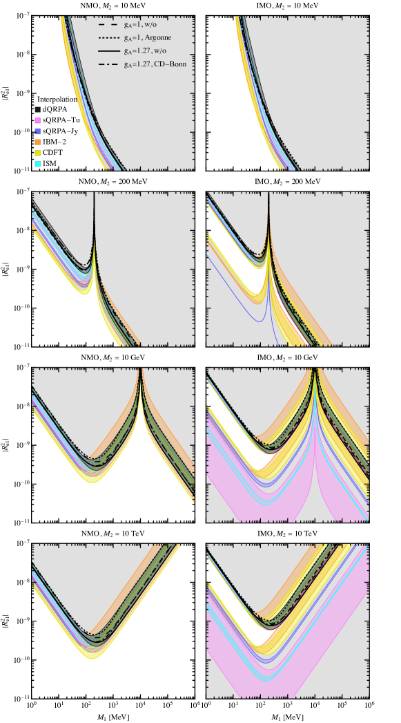
Figure 13: Sensitivity ranges of future $0\nu\beta\beta$ experiments to $M_{1}$ and $|R_{e1}^{2}|$ given fixed values of $M_{2}$ when we combine LEGEND-1000, SuperNEMO, SNO+II and nEXO by assuming $m_{\rm eff}^{\rm True}$= 0.

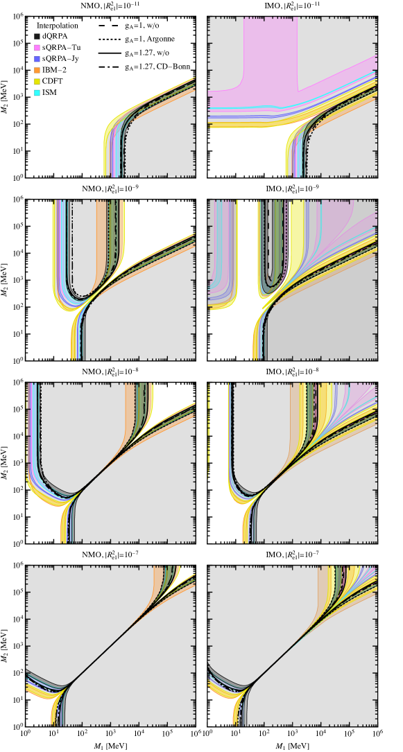
Figure 14: Sensitivity ranges of future experiments to $M_{1}$ and $M_{2}$ given fixed values of $|R_{e1}^{2}|$ when we combine LEGEND-1000, SuperNEMO, SNO+II and nEXO by assuming $m_{\rm eff}^{\rm True}$= 0.

4 Conclusion

In this work, we have discussed the Majorana neutrino mass dependent nuclear matrix element of the neutrinoless double beta decay and its implications for the minimal Type-I seesaw model. We have compared the explicit many-body calculations and naive extrapolations of the mass dependent NME and discussed their significant differences. We have derived limits on the parameter space of this model from the current $0\nu\beta\beta$ data, and compared with other experiments in a limiting case. Our results show that the constraints from $0\nu\beta\beta$ experiments is still the strongest one, and the NME plays a crucial role in determining the sensitivity of $0\nu\beta\beta$ experiments to the Majorana neutrino masses and mixing elements. Furthermore, the sensitive reach of future $0\nu\beta\beta$ proposals is also studied depending on various NME models. More parameter space of the minimal type-I seesaw is expected to be explored. Our work highlights the importance of accurate NME calculations for interpreting the experimental data and constraining new physics models. Further studies are needed to improve our understanding of NMEs and their uncertainties, as well as to explore other models beyond the minimal Type-I seesaw model.

5 Acknowledgements

Y.F. Li is grateful to Profs. Ke Han and Gaosong Li for helpful discussions on the CUORE and EXO-200 results respectively. The work of Y.F. Li and Y.Y. Zhang is supported by National Natural Science Foundation of China under Grant No. 12075255,  12075254 and No. 11835013. Y.Y. Zhang is also supported by China Postdoctoral Science Foundation funded project. D.L. Fang is supported by CAS from the “Light of West” program and the “from zero to one” program and by MOST from the National Key Research and Development Program of China (2021YFA1601300).

References

- (1) T. Kajita, Nobel Lecture: Discovery of atmospheric neutrino oscillations, Rev. Mod. Phys. 88 (2016), no. 3 030501.
- (2) A. B. McDonald, Nobel Lecture: The Sudbury Neutrino Observatory: Observation of flavor change for solar neutrinos, Rev. Mod. Phys. 88 (2016), no. 3 030502.
- (3) Z.-z. Xing, Flavor structures of charged fermions and massive neutrinos, Phys. Rept. 854 (2020) 1–147, [1909.09610].
- (4) P. Minkowski, at a Rate of One Out of Muon Decays?, Phys. Lett. B 67 (1977) 421–428.
- (5) T. Yanagida, Horizontal gauge symmetry and masses of neutrinos, Conf. Proc. C 7902131 (1979) 95–99.
- (6) M. Gell-Mann, P. Ramond, and R. Slansky, Complex Spinors and Unified Theories, Conf. Proc. C 790927 (1979) 315–321, [1306.4669].
- (7) S. L. Glashow, The Future of Elementary Particle Physics, NATO Sci. Ser. B 61 (1980) 687.
- (8) R. N. Mohapatra and G. Senjanovic, Neutrino Mass and Spontaneous Parity Nonconservation, Phys. Rev. Lett. 44 (1980) 912.
- (9) W. Konetschny and W. Kummer, Nonconservation of Total Lepton Number with Scalar Bosons, Phys. Lett. B 70 (1977) 433–435.
- (10) M. Magg and C. Wetterich, Neutrino Mass Problem and Gauge Hierarchy, Phys. Lett. B 94 (1980) 61–64.
- (11) J. Schechter and J. W. F. Valle, Neutrino Masses in SU(2) x U(1) Theories, Phys. Rev. D 22 (1980) 2227.
- (12) T. P. Cheng and L.-F. Li, Neutrino Masses, Mixings and Oscillations in SU(2) x U(1) Models of Electroweak Interactions, Phys. Rev. D 22 (1980) 2860.
- (13) R. N. Mohapatra and G. Senjanovic, Neutrino Masses and Mixings in Gauge Models with Spontaneous Parity Violation, Phys. Rev. D 23 (1981) 165.
- (14) G. Lazarides, Q. Shafi, and C. Wetterich, Proton Lifetime and Fermion Masses in an SO(10) Model, Nucl. Phys. B 181 (1981) 287–300.
- (15) R. Foot, H. Lew, X. G. He, and G. C. Joshi, Seesaw Neutrino Masses Induced by a Triplet of Leptons, Z. Phys. C 44 (1989) 441.
- (16) P. H. Frampton, S. L. Glashow, and T. Yanagida, Cosmological sign of neutrino CP violation, Phys. Lett. B 548 (2002) 119–121, [hep-ph/0208157].
- (17) Z.-z. Xing and Z.-h. Zhao, The minimal seesaw and leptogenesis models, Rept. Prog. Phys. 84 (2021), no. 6 066201, [2008.12090].
- (18) W.-l. Guo, Z.-z. Xing, and S. Zhou, Neutrino Masses, Lepton Flavor Mixing and Leptogenesis in the Minimal Seesaw Model, Int. J. Mod. Phys. E 16 (2007) 1–50, [hep-ph/0612033].
- (19) S. M. Bilenky and C. Giunti, Neutrinoless Double-Beta Decay: a Probe of Physics Beyond the Standard Model, Int. J. Mod. Phys. A 30 (2015), no. 04n05 1530001, [1411.4791].
- (20) M. J. Dolinski, A. W. P. Poon, and W. Rodejohann, Neutrinoless Double-Beta Decay: Status and Prospects, Ann. Rev. Nucl. Part. Sci. 69 (2019) 219–251, [1902.04097].
- (21) M. Agostini, G. Benato, J. A. Detwiler, J. Menéndez, and F. Vissani, Toward the discovery of matter creation with neutrinoless decay, Rev. Mod. Phys. 95 (2023), no. 2 025002, [2202.01787].
- (22) J. Engel and J. Menendez, Status and future of nuclear matrix elements for neutrinoless double-beta decay: A review, Rept.Prog.Phys. 80 (2017) 046301, [1610.06548].
- (23) J. M. Yao, J. Meng, Y. F. Niu, and P. Ring, Beyond-mean-field approaches for nuclear neutrinoless double beta decay in the standard mechanism, Prog. Part. Nucl. Phys. 126 (2022) 103965, [2111.15543].
- (24) E. J. Chun, A. Das, S. Mandal, M. Mitra, and N. Sinha, Sensitivity of Lepton Number Violating Meson Decays in Different Experiments, Phys. Rev. D 100 (2019), no. 9 095022, [1908.09562].
- (25) G. Isidori and F. Teubert, Status of indirect searches for New Physics with heavy flavour decays after the initial LHC run, Eur. Phys. J. Plus 129 (2014), no. 3 40, [1402.2844].
- (26) Y. Cai, T. Han, T. Li, and R. Ruiz, Lepton Number Violation: Seesaw Models and Their Collider Tests, Front. in Phys. 6 (2018) 40, [1711.02180].
- (27) KamLAND-Zen, A. Gando et al., Limit on Neutrinoless Decay of 136Xe from the First Phase of KamLAND-Zen and Comparison with the Positive Claim in 76Ge, Phys. Rev. Lett. 110 (2013), no. 6 062502, [1211.3863].
- (28) KamLAND-Zen, A. Gando et al., Search for Majorana Neutrinos near the Inverted Mass Hierarchy Region with KamLAND-Zen, Phys. Rev. Lett. 117 (2016), no. 8 082503, [1605.02889]. [Addendum: Phys.Rev.Lett. 117, 109903 (2016)].
- (29) KamLAND-Zen, S. Abe et al., First search for the majorana nature of neutrinos in the inverted mass ordering region with kamland-zen, Phys.Rev.Lett. 130 (3, 2023) 051801, [2203.02139].
- (30) EXO, M. Auger et al., Search for neutrinoless double-beta decay in 136xe with exo-200, Phys. Rev. Lett. 109 (2012) 032505, [1205.5608].
- (31) EXO-200, J. Albert et al., Search for majorana neutrinos with the first two years of exo-200 data, Nature 510 (2014) 229–234, [1402.6956].
- (32) EXO-200, J. Albert et al., Search for neutrinoless double-beta decay with the upgraded exo-200 detector, Phys.Rev.Lett. 120 (2018) 072701, [1707.08707].
- (33) EXO-200, G. Anton et al., Search for neutrinoless double-beta decay with the complete exo-200 dataset, Phys.Rev.Lett. 123 (2019) 161802, [1906.02723].
- (34) GERDA, M. Agostini et al., Results on Neutrinoless Double- Decay of 76Ge from Phase I of the GERDA Experiment, Phys. Rev. Lett. 111 (2013), no. 12 122503, [1307.4720].
- (35) M. Agostini et al., Background-free search for neutrinoless double- decay of 76Ge with GERDA, Nature 544 (2017) 47, [1703.00570].
- (36) M. Agostini et al., Improved limit on neutrinoless double beta decay of 76ge from gerda phase ii, Phys.Rev.Lett. 120 (2018) 132503, [1803.11100].
- (37) GERDA, M. Agostini et al., Probing majorana neutrinos with double- decay, Science 365 (2019) 1445, [1909.02726].
- (38) GERDA, M. Agostini et al., Final Results of GERDA on the Search for Neutrinoless Double- Decay, Phys. Rev. Lett. 125 (2020), no. 25 252502, [2009.06079].
- (39) C. Aalseth et al., Search for zero-neutrino double beta decay in 76ge with the majorana demonstrator, Phys.Rev.Lett. 120 (2018) 132502, [1710.11608].
- (40) Majorana, S. I. Alvis et al., A Search for Neutrinoless Double-Beta Decay in 76Ge with 26 kg-yr of Exposure from the MAJORANA DEMONSTRATOR, Phys. Rev. C 100 (2019), no. 2 025501, [1902.02299].
- (41) I. J. Arnquist et al., Final result of the majorana demonstrator’s search for neutrinoless double- decay in 76ge, Phys.Rev.Lett. 130 (7, 2023) 062501, [2207.07638].
- (42) CUORE, C. Alduino et al., First results from cuore: A search for lepton number violation via decay of 130te, Phys.Rev.Lett. 120 (2018) 132501, [1710.07988].
- (43) CUORE, D. Q. Adams et al., Improved limit on neutrinoless double-beta decay in 130te with cuore, Phys.Rev.Lett. 124 (2020) 122501, [1912.10966].
- (44) CUORE, D. Q. Adams et al., Search for Majorana neutrinos exploiting millikelvin cryogenics with CUORE, Nature 604 (2022), no. 7904 53–58, [2104.06906].
- (45) V. B. Brudanin et al., Search for double beta decay of Ca-48 in the TGV experiment, Phys. Lett. B 495 (2000) 63–68.
- (46) I. Ogawa, R. Hazama, H. Miyawaki, S. Shiomi, N. Suzuki, et al., Search for neutrino-less double beta decay of ca-48 by caf-2 scintillator, Nucl. Phys. A730 (2004) 215–223.
- (47) NEMO-3, R. Arnold et al., Measurement of the double-beta decay half-life and search for the neutrinoless double-beta decay of 48Ca with the NEMO-3 detector, Phys. Rev. D 93 (2016), no. 11 112008, [1604.01710].
- (48) R. Arnold et al., Final results on double beta decay to the ground state of from the NEMO-3 experiment, Eur. Phys. J. C 78 (2018), no. 10 821, [1806.05553].
- (49) NEMO, R. Arnold et al., First results of the search of neutrinoless double beta decay with the NEMO 3 detector, Phys. Rev. Lett. 95 (2005) 182302, [hep-ex/0507083].
- (50) H. Ejiri, K. Fushimi, K. Hayashi, T. Kishimoto, N. Kudomi, et al., Limits on the majorana neutrino mass and right-handed weak currents by neutrinoless double beta decay of mo-100, Phys. Rev. C63 (2001) 065501.
- (51) NEMO-3, R. Arnold et al., Search for neutrinoless double-beta decay of with the NEMO-3 detector, Phys. Rev. D 89 (2014), no. 11 111101, [1311.5695].
- (52) NEMO-3, R. Arnold et al., Results of the search for neutrinoless double- decay in 100Mo with the NEMO-3 experiment, Phys. Rev. D 92 (2015), no. 7 072011, [1506.05825].
- (53) V. Alenkov et al., First Results from the AMoRE-Pilot neutrinoless double beta decay experiment, Eur. Phys. J. C 79 (2019), no. 9 791, [1903.09483].
- (54) NEMO-3, R. Arnold et al., Measurement of the Decay Half-Life and Search for the Decay of 116Cd with the NEMO-3 Detector, Phys. Rev. D 95 (2017), no. 1 012007, [1610.03226].
- (55) NEMO, J. Argyriades et al., Measurement of the Double Beta Decay Half-life of Nd-150 and Search for Neutrinoless Decay Modes with the NEMO-3 Detector, Phys. Rev. C 80 (2009) 032501, [0810.0248].
- (56) NEMO-3, R. Arnold et al., Measurement of the 2 decay half-life of 150Nd and a search for 0 decay processes with the full exposure from the NEMO-3 detector, Phys. Rev. D 94 (2016), no. 7 072003, [1606.08494].
- (57) F. Pompa, T. Schwetz, and J.-Y. Zhu, Impact of nuclear matrix element calculations for current and future neutrinoless double beta decay searches, JHEP 06 (2023) 104, [2303.10562].
- (58) D.-L. Fang, Y.-F. Li, and Y.-Y. Zhang, Neutrinoless double beta decay in the minimal type-I seesaw model: How the enhancement or cancellation happens?, Phys. Lett. B 833 (2022) 137346, [2112.12779].
- (59) A. Faessler, M. González, S. Kovalenko, and F. Šimkovic, Arbitrary mass Majorana neutrinos in neutrinoless double beta decay, Phys. Rev. D 90 (2014), no. 9 096010, [1408.6077].
- (60) S. F. King, Large mixing angle MSW and atmospheric neutrinos from single right-handed neutrino dominance and U(1) family symmetry, Nucl. Phys. B 576 (2000) 85–105, [hep-ph/9912492].
- (61) Z.-z. Xing, Correlation between the Charged Current Interactions of Light and Heavy Majorana Neutrinos, Phys. Lett. B 660 (2008) 515–521, [0709.2220].
- (62) Z.-z. Xing, A full parametrization of the 6 X 6 flavor mixing matrix in the presence of three light or heavy sterile neutrinos, Phys. Rev. D 85 (2012) 013008, [1110.0083].
- (63) Z. Maki, M. Nakagawa, and S. Sakata, Remarks on the unified model of elementary particles, Prog. Theor. Phys. 28 (1962) 870–880.
- (64) B. Pontecorvo, Inverse beta processes and nonconservation of lepton charge, Zh. Eksp. Teor. Fiz. 34 (1957) 247.
- (65) F. Simkovic, G. Pantis, J. D. Vergados, and A. Faessler, Additional nucleon current contributions to neutrinoless double beta decay, Phys. Rev. C 60 (1999) 055502, [hep-ph/9905509].
- (66) M. Doi, T. Kotani, and E. Takasugi, Double beta Decay and Majorana Neutrino, Prog. Theor. Phys. Suppl. 83 (1985) 1.
- (67) J. Kotila and F. Iachello, Phase space factors for double- decay, Phys. Rev. C 85 (2012) 034316, [1209.5722].
- (68) V. Cirigliano, W. Dekens, J. De Vries, M. L. Graesser, E. Mereghetti, et al., New Leading Contribution to Neutrinoless Double- Decay, Phys. Rev. Lett. 120 (2018), no. 20 202001, [1802.10097].
- (69) R. Wirth, J. M. Yao, and H. Hergert, Ab Initio Calculation of the Contact Operator Contribution in the Standard Mechanism for Neutrinoless Double Beta Decay, Phys. Rev. Lett. 127 (2021), no. 24 242502, [2105.05415].
- (70) L. Jokiniemi, P. Soriano, and J. Menéndez, Impact of the leading-order short-range nuclear matrix element on the neutrinoless double-beta decay of medium-mass and heavy nuclei, Phys. Lett. B 823 (2021) 136720, [2107.13354].
- (71) Y. L. Yang and P. W. Zhao, A relativistic model-free prediction for neutrinoless double beta decay at leading order, 2308.03356.
- (72) F. Simkovic, A. Faessler, V. Rodin, P. Vogel, and J. Engel, Anatomy of nuclear matrix elements for neutrinoless double-beta decay, Phys. Rev. C 77 (2008) 045503, [0710.2055].
- (73) I. Esteban, M. C. Gonzalez-Garcia, M. Maltoni, T. Schwetz, and A. Zhou, The fate of hints: updated global analysis of three-flavor neutrino oscillations, JHEP 09 (2020) 178, [2007.14792].
- (74) D.-L. Fang, A. Faessler, and F. Simkovic, 0 -decay nuclear matrix element for light and heavy neutrino mass mechanisms from deformed quasiparticle random-phase approximation calculations for 76Ge, 82Se, 130Te, 136Xe , and 150Nd with isospin restoration, Phys. Rev. C 97 (2018), no. 4 045503, [1803.09195].
- (75) F. Šimkovic, V. Rodin, A. Faessler, and P. Vogel, 0 and 2 nuclear matrix elements, quasiparticle random-phase approximation, and isospin symmetry restoration, Phys. Rev. C 87 (2013), no. 4 045501, [1302.1509].
- (76) Particle Data Group, P. A. Zyla et al., Review of Particle Physics, PTEP 2020 (2020), no. 8 083C01.
- (77) J. Hyvärinen and J. Suhonen, Nuclear matrix elements for decays with light or heavy Majorana-neutrino exchange, Phys. Rev. C 91 (2015), no. 2 024613.
- (78) D.-L. Fang, A. Faessler, V. Rodin, and F. Simkovic, Neutrinoless double beta decay of deformed nuclei within QRPA with realistic interaction, Phys. Rev. C 83 (2011) 034320, [1101.2149].
- (79) J. Barea, J. Kotila, and F. Iachello, Nuclear matrix elements for double- decay, Phys. Rev. C 87 (2013), no. 1 014315, [1301.4203].
- (80) L. S. Song, J. M. Yao, P. Ring, and J. Meng, Nuclear matrix element of neutrinoless double- decay: Relativity and short-range correlations, Phys. Rev. C 95 (2017), no. 2 024305, [1702.02448].
- (81) J. Menéndez, Neutrinoless decay mediated by the exchange of light and heavy neutrinos: The role of nuclear structure correlations, J. Phys. G 45 (2018), no. 1 014003, [1804.02105].
- (82) P. K. Rath, R. Chandra, K. Chaturvedi, P. Lohani, P. K. Raina, et al., Neutrinoless decay transition matrix elements within mechanisms involving light Majorana neutrinos, classical Majorons, and sterile neutrinos, Phys. Rev. C 88 (2013), no. 6 064322, [1308.0460].
- (83) N. Hinohara and J. Engel, Proton-Neutron Pairing Amplitude as a Generator Coordinate for Double-Beta Decay, Phys. Rev. C 90 (2014), no. 3 031301, [1406.0560].
- (84) J. Menendez, A. Poves, E. Caurier, and F. Nowacki, Disassembling the Nuclear Matrix Elements of the Neutrinoless beta beta Decay, Nucl. Phys. A 818 (2009) 139–151, [0801.3760].
- (85) P. Gysbers et al., Discrepancy between experimental and theoretical -decay rates resolved from first principles, Nature Phys. 15 (2019), no. 5 428–431, [1903.00047].
- (86) M. T. Mustonen and J. Engel, Large-scale calculations of the double- decay of , and in the deformed self-consistent Skyrme quasiparticle random-phase approximation, Phys. Rev. C 87 (2013), no. 6 064302, [1301.6997].
- (87) J. Barea, J. Kotila, and F. Iachello, and nuclear matrix elements in the interacting boson model with isospin restoration, Phys. Rev. C 91 (2015), no. 3 034304, [1506.08530].
- (88) J. M. Yao, L. S. Song, K. Hagino, P. Ring, and J. Meng, Systematic study of nuclear matrix elements in neutrinoless double- decay with a beyond-mean-field covariant density functional theory, Phys. Rev. C 91 (2015), no. 2 024316, [1410.6326].
- (89) B. A. Brown, D. L. Fang, and M. Horoi, Evaluation of the theoretical nuclear matrix elements for decay of 76Ge, Phys. Rev. C 92 (2015), no. 4 041301.
- (90) A. Caldwell, M. Ettengruber, A. Merle, O. Schulz, and M. Totzauer, Global Bayesian analysis of neutrino mass data, Phys. Rev. D 96 (2017), no. 7 073001, [1705.01945].
- (91) S. D. Biller, Combined constraints on Majorana masses from neutrinoless double beta decay experiments, Phys. Rev. D 104 (2021), no. 1 012002, [2103.06036].
- (92) F. Capozzi, E. Di Valentino, E. Lisi, A. Marrone, A. Melchiorri, et al., Unfinished fabric of the three neutrino paradigm, Phys. Rev. D 104 (2021), no. 8 083031, [2107.00532].
- (93) E. Lisi and A. Marrone, Majorana neutrino mass constraints in the landscape of nuclear matrix elements, Phys. Rev. D 106 (2022), no. 1 013009, [2204.09569].
- (94) E. Lisi, A. Marrone, and N. Nath, Interplay between noninterfering neutrino exchange mechanisms and nuclear matrix elements in 0 decay, Phys. Rev. D 108 (2023), no. 5 055023, [2306.07671].
- (95) T2K, K. Abe et al., Search for heavy neutrinos with the T2K near detector ND280, Phys. Rev. D 100 (2019), no. 5 052006, [1902.07598].
- (96) MicroBooNE, P. Abratenko et al., Search for Heavy Neutral Leptons Decaying into Muon-Pion Pairs in the MicroBooNE Detector, Phys. Rev. D 101 (2020), no. 5 052001, [1911.10545].
- (97) M. Lindner, M. Platscher, and F. S. Queiroz, A Call for New Physics : The Muon Anomalous Magnetic Moment and Lepton Flavor Violation, Phys. Rept. 731 (2018) 1–82, [1610.06587].
- (98) NA62, E. Cortina Gil et al., Search for heavy neutral lepton production in decays to positrons, Phys. Lett. B 807 (2020) 135599, [2005.09575].
- (99) CHARM, F. Bergsma et al., A Search for Decays of Heavy Neutrinos in the Mass Range 0.5-GeV to 2.8-GeV, Phys. Lett. B 166 (1986) 473–478.
- (100) Belle, D. Liventsev et al., Search for heavy neutrinos at Belle, Phys. Rev. D 87 (2013), no. 7 071102, [1301.1105]. [Erratum: Phys.Rev.D 95, 099903 (2017)].
- (101) DELPHI, P. Abreu et al., Search for neutral heavy leptons produced in Z decays, Z. Phys. C 74 (1997) 57–71. [Erratum: Z.Phys.C 75, 580 (1997)].
- (102) ATLAS, G. Aad et al., Search for heavy neutral leptons in decays of bosons produced in 13 TeV collisions using prompt and displaced signatures with the ATLAS detector, JHEP 10 (2019) 265, [1905.09787].
- (103) CMS, A. M. Sirunyan et al., Search for heavy neutral leptons in events with three charged leptons in proton-proton collisions at 13 TeV, Phys. Rev. Lett. 120 (2018), no. 22 221801, [1802.02965].
- (104) LEGEND, N. Abgrall et al., The Large Enriched Germanium Experiment for Neutrinoless Decay: LEGEND-1000 Preconceptual Design Report, 2107.11462.
- (105) SuperNEMO, M. Kauer, Calorimeter \& for the SuperNEMO Double Beta Decay Experiment, J. Phys. Conf. Ser. 160 (2009) 012031, [0807.2188].
- (106) SNO+, V. Albanese et al., The SNO+ experiment, JINST 16 (2021), no. 08 P08059, [2104.11687].
- (107) nEXO, G. Adhikari et al., nEXO: neutrinoless double beta decay search beyond 1028 year half-life sensitivity, J. Phys. G 49 (2022), no. 1 015104, [2106.16243].