Guided Discrete Diffusion for Electronic Health Record Generation

Abstract

Electronic health records (EHRs) are a pivotal data source that enables numerous applications in computational medicine, e.g., disease progression prediction, clinical trial design, and health economics and outcomes research. Despite wide usability, their sensitive nature raises privacy and confidentially concerns, which limit potential use cases. To tackle these challenges, we explore the use of generative models to synthesize artificial, yet realistic EHRs. While diffusion-based methods have recently demonstrated state-of-the-art performance in generating other data modalities and overcome the training instability and mode collapse issues that plague previous GAN-based approaches, their applications in EHR generation remain underexplored. The discrete nature of tabular medical code data in EHRs poses challenges for high-quality data generation, especially for continuous diffusion models. To this end, we introduce a novel tabular EHR generation method, EHR-D3PM, which enables both unconditional and conditional generation using the discrete diffusion model. Our experiments demonstrate that EHR-D3PM significantly outperforms existing generative baselines on comprehensive fidelity and utility metrics while maintaining less membership vulnerability risks. Furthermore, we show EHR-D3PM is effective as a data augmentation method and enhances performance on downstream tasks when combined with real data.

1 Introduction

Electronic health records (EHRs) are a rich and comprehensive data source, enabling numerous applications in computational medicine including the development of models for disease progression prediction and clinical event medical models (Li et al., 2020; Rajkomar et al., 2018), clinical trial design (Bartlett et al., 2019) and health economics and outcome research (Padula et al., 2022). In particular, many existing disease prediction models primarily utilize tabular formats, often transforming longitudinal EHR data into binary or categorical forms, rather than employing time-series forecasting methods (Lee et al., 2022; Huang et al., 2021; Rao et al., 2023; Debal and Sitote, 2022). However, the sensitive nature of EHRs, which includes confidential medical data, poses challenges for their broad use due to privacy concerns and patient confidentiality requirements (Hodge Jr et al., 1999). In addition to these concerns, data scarcity also restricts their potential use in applications for rare medical conditions. To address these challenges, we consider using generative models to synthesize artificial, but realistic EHRs, which has recently emerged as a crucial research area for advancing applications of machine learning to healthcare and other industries with privacy and data scarcity challenges.

The primary goal of synthetic EHR generation is to generate data that is (i) indistinguishable from real data to an expert, but (ii) not attributable to any actual patients. Recent advancements in deep generative models, including Variational Autoencoders (VAE) (Vincent et al., 2008) and Generative Adversarial Networks (GAN) (Goodfellow et al., 2014), have demonstrated significant promise in generating realistic synthetic EHR data (Biswal et al., 2021; Choi et al., 2017a). In particular, GAN-based EHR generation has emerged as the most predominant and popular approach (Choi et al., 2017a; Zhang et al., 2020; Torfi and Fox, 2020a), and achieved state-of-the-art performance in terms of quality and privacy preservation. However, the unstable training process of GAN-based methods can lead to mode collapse, raising concerns about their widespread application.

Recently, diffusion-based generative models, initially introduced by Sohl-Dickstein et al. (2015), have demonstrated impressive capabilities in generating high-quality samples in various domains, including images (Ho et al., 2020; Song and Ermon, 2020), audio (Chen et al., 2020; Kong et al., 2020), and text (Hoogeboom et al., 2021b; Austin et al., 2021; Chen et al., 2023). A diffusion model consists of a forward process, which gradually transforms training data into pure noise, and a reverse sampling process that reconstructs data from noise using a learned network. Compared to GANs, their training is more stable as it only involves maximizing the log-likelihood of a single neural network.

Due to the superior performance of diffusion models, recent methods have explored their application in generating categorical EHR data (Yuan et al., 2023; Ceritli et al., 2023). While these approaches demonstrate promising performance, their improvement over previous GAN-based methods is varied. Particularly, they struggle to generate EHR records with rare medical conditions at rates consistent with the occurrence of such conditions in real-world data. Furthermore, existing approaches offer limited support for conditional generation, which is crucial for many downstream tasks such as disease classification.

In this paper, we propose a novel EHR generation method that utilizes discrete diffusion (Sohl-Dickstein et al., 2015; Hoogeboom et al., 2021b; Austin et al., 2021; Chen et al., 2023), a type of diffusion process tailored for discrete data sampling, as well as a flexible conditional sampling method that does not require additional model training. Our contributions are summarized as follows:

• We introduce a Discrete Denoising Diffusion model specifically tailed for generation of tabular medical codes in EHRs, dubbed EHR-D3PM. Our method incorporates an architecture that effectively captures feature correlations, enhancing the generation process and achieving state-of-the-art performance. Notably, EHR-D3PM excels in generating instances of rare conditions, an aspect where existing methods often face challenges.

• We further extend EHR-D3PM to conditional generation, specifically tailored for generating EHR samples related to particular medical conditions. Given the unique requirements of this task and the discrete nature of EHR data, we have custom-designed the energy function and applied energy-guided Langevin dynamics at the latent layer of the predictor network to achieve this goal.

• We investigate the effectiveness of EHR-D3PM as a data augmentation method in downstream tasks. We show that synthetic EHR data generated by EHR-D3PM yields comparable performance to that of real data in terms of AUPRC and AUROC when used to train predictive models and when combined with the real data, EHR-D3PM can enhance the performance of predictive models.

Notation. We use the symbol $\mathbf{q}$ to denote the real distribution in a diffusion process, while $\mathbf{p}_{\bm{\theta}}$ represents the distribution parameterized by the NN during sampling. With its success probability inside the parentheses, the Bernoulli distribution is denoted by $\mathrm{Bernoulli}(\cdot)$. We further use $\mathrm{Cat}(\mathbf{p})$ to denote a categorical distribution over a one-hot row vector with probabilities given by the row vector $\mathbf{p}$.

2 Related Work

EHR Synthesis. Various methods have been developed for generating synthetic EHR data. Buczak et al. (2010) proposed an early data-driven approach for creating synthetic EHRs, but their approach offers limited flexibility has privacy concerns. Recently, GANs have become prominent in EHR generation, including medGAN Choi et al. (2017b), medBGAN (Baowaly et al., 2018), EHRWGAN (Zhang et al., 2019), and CorGAN Torfi and Fox (2020b). GAN-based methods offer significant improvement in the quality of synthetic EHRs, but often face issues related to training instability and mode collapse (Thanh-Tung et al., 2018), restricting their wide use and the diversity of generated data. To address this, other methods, including variational auto-encoders (Biswal et al., 2020) and language models (Wang and Sun, 2022), have been explored. Very recently, MedDiff (He et al., 2023) and EHRdiff (Yuan et al., 2023) considered using diffusion models and proposed sampling techniques for high-quality EHR generation. Ceritli et al. (2023) further extended the diffusion model to mixed-type EHRs. In this paper, we focus on developing a guided discrete diffusion model specifically designed for generating tabular medical codes in EHRs and improving the generation of codes for rare conditions, which previous methods struggle at.

Discrete Diffusion Models. The study of discrete diffusion models was pioneered by Sohl-Dickstein et al. (2015), which explored diffusion processes in binary random variables. The approach was further developed by Ho et al. (2020); Song et al. (2020), which incorporates categorical random variables using transition matrices with uniform probabilities. Subsequently, Austin et al. (2021) introduced a generalized framework named Discrete Denoising Diffusion Probabilistic Models (D3PMs) for categorical random variables, effectively combining discrete diffusion models with Masked Language Models (MLMs). Recent advancements in this field include the introduction of editing-based operations (Jolicoeur-Martineau et al., 2021; Reid et al., 2022), auto-regressive diffusion models (Hoogeboom et al., 2021a; Ye et al., 2023), a continuous-time structure (Campbell et al., 2022), strides in generation acceleration (Chen et al., 2023), and the application of neural network analogs for learning purposes (Sun et al., 2022). In this paper, we focus on the D3PMs with multinomial distribution.

3 Background

In this section, we provide background on diffusion models.

Diffusion Model. Given $\mathbf{x}_{0}$ drawn from a target data distribution following $q_{\mathrm{data}}(\cdot)$, the forward process is a Markov process that maps the clean data $\mathbf{x}_{0}$ to a noisy sample from a prior distribution $q_{\mathrm{noise}}(\cdot)$. The process $\mathbf{x}_{0}\rightarrow\mathbf{x}_{T}$ is composed of the conditional distributions $q(\mathbf{x}_{t}|\mathbf{x}_{t-1},\mathbf{x}_{0})$ where

$$q(\mathbf{x}_{1:T}|\bm{x}_{0})=\prod_{t=1}^{T}q(\mathbf{x}_{t}|\mathbf{x}_{t-1},\mathbf{x}_{0}).$$ (1)

By Bayes rule, (1) induces a reverse process $\mathbf{x}_{T}\rightarrow\mathbf{x}_{0}$ that can convert samples from the prior $q_{\mathrm{noise}}$ into samples from the target distribution $q_{\mathrm{data}}$,

$$q(\mathbf{x}_{t-1}|\mathbf{x}_{t},\mathbf{x}_{0})=\frac{q(\mathbf{x}_{t}|\mathbf{x}_{t-1},\mathbf{x}_{0})q(\mathbf{x}_{t-1}|\mathbf{x}_{0})}{q(\mathbf{x}_{t}|\mathbf{x}_{0})}.$$ (2)

After training a diffusion model, the reverse process can be used for synthetic data generation by sampling from the noise distribution $q_{\mathrm{noise}}$ and repeatedly applying a learnt predictor (neural network) $p_{\bm{\theta}}(\cdot|\mathbf{x}_{t})$ parameterized by $\bm{\theta}$:

$$p_{\bm{\theta}}(\mathbf{x}_{T}) =q_{\mathrm{noise}}(\mathbf{x}_{T})$$

$$p_{\bm{\theta}}(\mathbf{x}_{t-1}|\mathbf{x}_{t}) =\int_{\widehat{\mathbf{x}}_{0}}q(\mathbf{x}_{t-1}|\mathbf{x}_{t},\widehat{\mathbf{x}}_{0})p_{\bm{\theta}}(\widehat{\mathbf{x}}_{0}|\mathbf{x}_{t})d\widehat{\mathbf{x}}_{0}.$$ (3)

Training Objective. The neural network $p_{\bm{\theta}}(\cdot|\mathbf{x}_{t})$ in (3) that predicts $\widehat{\mathbf{x}}_{0}$ is trained by maximizing the evidence lower bound (ELBO) (Sohl-Dickstein et al., 2015),

$$\log p_{\theta}(\mathbf{x}_{0}) \geq\mathbb{E}_{q(\mathbf{x}_{1:T}|\mathbf{x}_{0})}\Big{[}\log\frac{p(\mathbf{x}_{0:T})}{q(\mathbf{x}_{1:T}|\mathbf{x}_{0})}\Big{]}d\mathbf{x}_{1:T}$$

$$=\mathbb{E}_{q(\mathbf{x}_{1}|\mathbf{x}_{0})}[\log p_{\bm{\theta}}(\mathbf{x}_{0}|\mathbf{x}_{1})]$$

$$-\sum_{t=2}^{T}\mathbb{E}_{q(\mathbf{x}_{t}|\mathbf{x}_{0})}[\mathrm{KL}(q(\mathbf{x}_{t-1}|\mathbf{x}_{t},\mathbf{x}_{0})\|p_{\bm{\theta}}(\mathbf{x}_{t-1}|\mathbf{x}_{t}))$$

$$-\mathbb{E}_{q(\mathbf{x}_{T}|\mathbf{x}_{0})}\mathrm{KL}(q(\mathbf{x}_{T}|\mathbf{x}_{0})\|p_{\bm{\theta}}(\mathbf{x}_{T})),$$

Here KL denotes Kullback-Liebler divergence and the last term $\mathbb{E}_{q(\mathbf{x}_{T}|\mathbf{x}_{0})}\mathrm{KL}(q(\mathbf{x}_{T}|\mathbf{x}_{0})\|q_{\mathrm{noise}}(\mathbf{x}_{T}))$ equals or approximately equals zero if the diffusion process $q$ is properly designed.

Different choices of diffusion process (1) and (2) will result in different sampling methods (3). There are two popular approaches to constructing a diffusion generative model, depending on the nature of the process.

Gaussian Diffusion Process. The Gaussian diffusion process assumes a Gaussian noise distribution $\mathbf{q}_{\mathrm{noise}}$. In particular, the prior is chosen to be $q_{\mathrm{noise}}=\mathcal{N}(0,\mathbf{I})$, and the forward process is characterized by

$$q(\mathbf{x}_{t}|\mathbf{x}_{t-1},\mathbf{x}_{0})=\mathcal{N}(\mathbf{x}_{t};\sqrt{1-\beta_{t}}\mathbf{x}_{t-1},\beta_{t}\mathbf{I}),$$

where $\beta_{t}$ is the variance schedule determined by a pre-specified corruption schedule. The Gaussian diffusion process has achieved great success in continuous-valued applications like image generation (Ho et al., 2020; Song et al., 2020). Recently, it has been applied to tabular EHR data generation (He et al., 2023; Yuan et al., 2023).

Discrete Diffusion Process. Discrete Denoising Diffusion Probabilistic Models (D3PMs) is designed to generate categorical data from a vocabulary $\{1,\ldots,K\}$, represented as a one-hot vector $\mathbf{x}\in\{0,1\}^{K}$. The noise follows a categorical distribution $\mathbf{q}_{\mathrm{noise}}$. The Multinomial distribution (Hoogeboom et al., 2021b) is among the most effective noise distributions. In particular, $\mathbf{q}_{\mathrm{noise}}$ is chosen to be a uniform distribution over the one-hot basis of the vocabulary $\{\mathbf{e}_{1},\ldots,\mathbf{e}_{K}\}$, and the forward process is characterized by

$$q(\mathbf{x}_{t}|\mathbf{x}_{t-1},\mathbf{x}_{0})=\mathrm{Cat}\big{(}\mathbf{x}_{t};\beta_{t}\mathbf{x}_{t-1}+(1-\beta_{t})\mathbf{q}_{\mathrm{noise}}\big{)},$$

where $\mathrm{Cat}$ is the categorical distribution and $\beta_{t}$ is the variance schedule determined by a pre-specified corruption schedule. Due to its discrete nature, D3PM is widely used to generate categorical data like text (Hoogeboom et al., 2021b; Austin et al., 2021) and categorical tabular data Kotelnikov et al. (2023); Ceritli et al. (2023). This paper uses a D3PM with a multinomial noise distribution to generate tabular medical codes in EHRs.

4 Method

In this section, we formalize the problem of tabular EHR data generation and provide the technical details of our method.

4.1 Problem Formulation

We consider medical coding data in EHRs, such as ICD codes, which are standardized codes published by the World Health Organization that correspond to specific medical diagnoses and procedures (Slee, 1978). While we focus on ICD codes specifically, our approach can be used with other medical coding data, e.g., CPT, NDC and LOINC codes. For a given (usually high dimensional) set $\Omega$ of ICD codes of interest, we encode the set as $N:=|\Omega|$ categories $\{1,2,\ldots,N\}$. A sample patient EHR $\mathbf{x}$ is then encoded as a sequence of $N$ tokens $\mathbf{x}=[\mathbf{x}^{(1)},\ldots,\mathbf{x}^{(N)}]$, where each token $\mathbf{x}^{(i)}\in\{0,1\}^{2}$ is a one-hot function. $\mathbf{x}^{(i)}$ represents the occurrence of the $i$-th ICD code in the patient EHR. In particular, $\mathbf{x}^{(i)}=[1,0]$ represents occurrence of code and $\mathbf{x}^{(i)}=[0,1]$ represents its absence. We assume a sufficiently large set of patient EHRs is available to train a multinomial diffusion model to generate artificial encoded patient EHRs sequences $\mathbf{x}^{\prime}$.

4.2 Unconditional Generation

In Section 3, we introduced multinomial diffusion with a single token, $\mathbf{x}\in\mathbb{R}^{K}$. In the context of categorical EHRs, we aim to generate a sequence of $N$ tokens with $K=2$, denoted by $\mathbf{x}=[\mathbf{x}^{(1)},\ldots,\mathbf{x}^{(N)}]$. Therefore, we need to extend the terminology from Section 3. We define the sequence of tokens at the $t$-th time step as $\mathbf{x}_{t}=[\mathbf{x}_{t}^{(1)},\ldots,\mathbf{x}_{t}^{(N)}]$, where $\mathbf{x}_{t}^{(i)}$ represents the $i$-th token at diffusion step $t$. Multinomial noise $\mathbf{q}_{\mathrm{noise}}$ is added to each token in the sequence independently during the diffusion process,

$$q(\mathbf{x}_{t}|\mathbf{x}_{t-1},\mathbf{x}_{0})=\prod_{i=1}^{N}\mathrm{Cat}\big{(}\mathbf{x}_{t}^{(i)};\beta_{t}\mathbf{x}_{t-1}^{(i-1)}+(1-\beta_{t})\mathbf{q}_{\mathrm{noise}}\big{)}.$$

The reverse sampling procedure uses the predictor $p_{\bm{\theta}}(\cdot|\mathbf{x}_{t})$ with the following neural network architecture:

$$\mathbf{z}_{0,t} =\mathbf{x}_{t}=[\mathbf{x}_{t}^{(1)},\ldots,\mathbf{x}_{t}^{(N)}]$$

$$\mathbf{z}_{l,t}^{\prime\prime} =[\mathbf{z}_{l-1,t}^{(1)},\ldots,\mathbf{z}_{l-1,t}^{(N)}]+\mathbf{E}_{\mathrm{pos}}+\mathbf{E}_{\mathrm{time}},$$

$$\mathbf{z}_{l,t}^{\prime} =\mathrm{LinMSA}(\mathrm{LN}(\mathbf{z}^{\prime\prime}_{l-1,t}))+\mathbf{z}^{\prime\prime}_{l-1,t},$$

$$\mathbf{z}_{L,t} =\mathrm{ParallelMLP}(\mathrm{LN}(\mathbf{z}_{L-1,t}^{\prime})),$$

$$\mathrm{Output} =[\mathrm{softmax}(\mathbf{z}_{L,t}^{(1)}),\ldots,\mathrm{softmax}(\mathbf{z}_{L,t}^{(N)})]$$ (4)

where $\mathbf{E}_{\mathrm{pos}},\mathbf{E}_{\mathrm{time}}\in\mathbb{R}^{2\times D}$ represents the position embedding and time embedding respectively, the variable $l$ indexes the layers belonging to the set $\{1,\ldots,L\}$, $\mathrm{LinMSA}$ refers to the linear-time multi-head self-attention block proposed by Wang et al. (2020) and $\mathrm{LN}$ is an abbreviation for layer normalization. For each dimension of $\widehat{\mathbf{x}}_{0}$, we apply a multilayer perceptron layer to obtain the logit, abbreviated as ParallelMLP. The $\mathrm{softmax}$ function transforms the last-layer latent variable $\mathbf{z}_{L}^{i}$ into the conditional probability $p_{\bm{\theta}}(\cdot|\mathbf{x}_{t})$, serving as the final softmax layer. The details of our denoise model are provided in Fig. 6 in Appendix A.2.

4.3 Conditional Generation with Classifier Guidance

The goal of conditional generation is to generate $p_{\bm{\theta}}(\mathbf{x}|\mathbf{c})$ close to $q_{\mathrm{data}}(\mathbf{x}|\mathbf{c})$, where $\mathbf{c}$ denotes a context, such as the presence of a single or group of ICD codes in a patient EHR. $\mathbf{c}$ is not available at training time, but we assume access to a classifier $p(\mathbf{c}|\mathbf{x})$ that is close to the conditional distribution $q_{\mathrm{data}}(\mathbf{c}|\mathbf{x})$. Then given an unconditional EHR generator $p_{\bm{\theta}}(\mathbf{x})$ and classifier $p(\mathbf{c}|\mathbf{x})$, we propose a training-free conditional generator as follows

$$p_{\bm{\theta}}(\mathbf{x}|\mathbf{c})\propto p_{\bm{\theta}}(\mathbf{x})\cdot p(\mathbf{c}|\mathbf{x}).$$ (5)

Since $q_{\mathrm{data}}(\mathbf{x}|\mathbf{c})\propto q_{\mathrm{data}}(\mathbf{x})\cdot q_{\mathrm{data}}(\mathbf{c}|\mathbf{x})$, we can expect $p_{\bm{\theta}}(\mathbf{x}|\mathbf{c})$ in (5) is close to $q_{\mathrm{data}}(\mathbf{x}|\mathbf{c})$ provided the unconditional generator $p_{\bm{\theta}}(\mathbf{x})$ is close to $q_{\mathrm{data}}(\mathbf{x})$ and the classifier $p(\mathbf{c}|\mathbf{x})$ is close to $q_{\mathrm{data}}(\mathbf{c}|\mathbf{x})$.

To sample from (5), we apply the following guided multinomial diffusion procedure:

$$p_{\bm{\theta}}(\mathbf{x}_{t-1}|\mathbf{x}_{t},\mathbf{c})=\sum_{\widehat{\mathbf{x}}_{0}}q(\mathbf{x}_{t-1}|\widehat{\mathbf{x}}_{0},\mathbf{x}_{t})p_{\bm{\theta}}(\widehat{\mathbf{x}}_{0}|\mathbf{x}_{t},\mathbf{c}),$$

where $\widehat{\mathbf{x}}_{0}$ is the latent variable that predicts $\mathbf{x}_{0}$. Since $\widehat{\mathbf{x}}_{0}$ lies in a discrete space, we cannot directly use the Langevin dynamics in the space of $\widehat{\mathbf{x}}_{0}$. However, the last-layer latent variable $\mathbf{z}_{L,t}$ in (4) (before the softmax layer) lies in a continuous space. We have the following:

$$p_{\bm{\theta}}(\widehat{\mathbf{x}}_{0}|\mathbf{x}_{t},\mathbf{c})=\int p_{\bm{\theta}}(\widehat{\mathbf{x}}_{0}|\mathbf{z}_{L,t})p_{\bm{\theta}}(\mathbf{z}_{L,t}|\mathbf{x}_{t},\mathbf{c})d\mathbf{z}_{L}.$$

Therefore, we can use the plug-and-play method (Dathathri et al., 2019) with the latent space $\mathbf{z}_{L}$, which has been recently employed in text generation (Dathathri et al., 2019) and protein design (Gruver et al., 2023). In particular, we introduce a modified latent variable $\mathbf{y}^{(k)}$ for $\mathbf{z}_{L,t}$, which is initialized as $\mathbf{y}^{(0)}\leftarrow\mathbf{z}_{L,t}$. Then we iterative apply the following update with Langevin dynamics

$$\mathbf{y}^{(k+1)}\leftarrow\mathbf{y}^{(k)}-\eta\nabla_{\mathbf{y}^{(k)}}[\mathcal{D}_{\mathrm{KL}}(\mathbf{y}^{(k)})-V_{\bm{\theta}}(\mathbf{y}^{(k)})]+\sqrt{2\eta\tau}\bm{\epsilon},$$

where the energy function $V_{\bm{\theta}}(\mathbf{y}^{(k)})=\log(p(\mathbf{c}|\mathbf{y}^{(k)}))=\log\big{(}\sum_{\widehat{\mathbf{x}}_{0}}p_{\bm{\theta}}(\widehat{\mathbf{x}}_{0}|\mathbf{y}^{(k)})p(\mathbf{c}|\widehat{\mathbf{x}}_{0})\big{)}$ and $\mathcal{D}_{\mathrm{KL}}(\mathbf{y}^{(k)})=\lambda\mathrm{KL}(p_{\theta}(\widehat{\mathbf{x}}_{0}|\mathbf{y}^{(k)})||p_{\theta}(\widehat{\mathbf{x}}_{0}|\mathbf{y}^{(0)}))$ is the Kullback–Leibler ($\mathrm{KL}$) divergence for regularization of the guided Markov transition. The gradient of the energy term $\nabla_{\mathbf{y}^{(k)}}V_{\bm{\theta}}$ drives the hidden state $\mathbf{y}^{(k)}$ towards high probability of $p(\mathbf{c}|\mathbf{y}^{(k)})$. The gradient of the regularization term $\nabla_{\mathbf{y}^{(k)}}\mathcal{D}_{\mathrm{KL}}$ ensures the guided transition distribution still maximizes the likelihood of the diffusion model. For a more detailed discussion, see Appendix C.

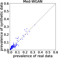
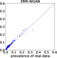
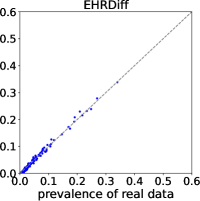
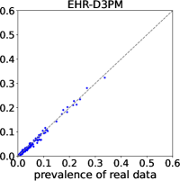
(a) Spearm corr = 0.82	(b) Spearm corr = 0.83	(c) Spearm corr = 0.75	(d) Spearm corr = 0.94
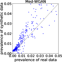
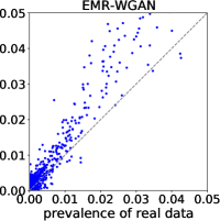
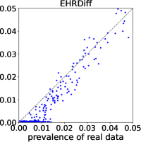
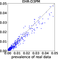
(e) Spearm corr = 0.79	(f) Spearm corr = 0.80	(g) Spearm corr = 0.71	(h) Spearm corr = 0.93

Figure 1: Comparison of prevalence in synthetic data and real data (MIMIC). The second row represents the prevalence of the first row in the low data regime. The prevalence is computed on 10K samples as the MIMIC dataset is relatively small. The dashed diagonal lines represent the perfect matching of code prevalence between synthetic data and real EHR data. Pearson correlations are very high for all methods and thus not used as a metric to compare different methods.

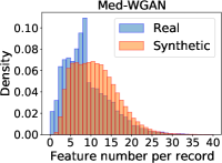
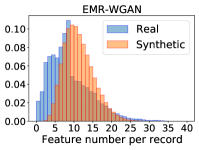
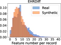
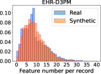
Figure 2: Density comparison of per-record feature number for synthetic and real data for the MIMIC dataset. The number of features per record is the sum of ICD codes present in each sample. The number of bins is 40, and the range of feature number values is (0, 40).

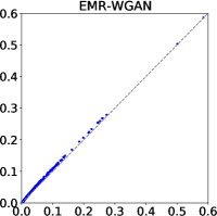
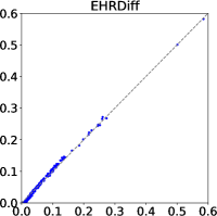
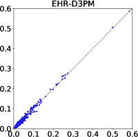
(a) Spearm corr = 0.91	(b) Spearm corr = 0.98	(c) Spearm corr = 0.85	(d) Spearm corr = 0.99
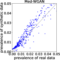
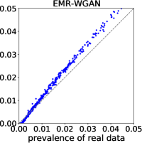
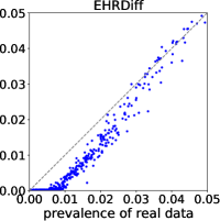
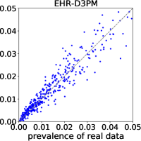
(e) Spearm corr = 0.87	(f) Spearm corr = 0.91	(g) Spearm corr = 0.79	(h) Spearm corr = 0.97

Figure 3: Comparison of prevalence in synthetic data and real data $\mathcal{D}_{1}$. The second row represents the prevalence of the first row in the low data regime. The prevalence is computed on 200K samples. The dashed diagonal lines represent the perfect matching of code prevalence between synthetic data and real EHR data. Spearman correlations between synthetic data and real data are reported.

5 Experiments

In this section, we apply our method to three EHR datasets, including the widely used public MIMIC-III dataset and two larger private datasets from a large health institute. We compare our method to popular and state-of-the-art EHR generative models in terms of fidelity, utility and privacy.

5.1 Experiment Setup

Datasets. Public Datasets MIMIC-III (Johnson et al., 2016) includes deidentified patient EHRs from hospital stays. For each patient’s EHR, we extract the diagnosis and procedure ICD-9 codes and truncate the codes to the first three digits. This dataset includes a patient population of size 46,520. Private Datasets We consider two private datasets of patient EHRs from a large healthcare institution. For each, we extract the diagnosis and procedure ICD-10 codes and truncate the codes to the first three digits. The first dataset, denoted by $\mathcal{D}_{1}$, includes a patient population of size 1,670,347 and has sparse binary features; the second dataset, denoted by $\mathcal{D}_{2}$, includes a patient population of size 1,859,536 and has relatively denser binary features from a different corpus.

Diseases of Interest. To investigate the utility of our proposed method, we consider using the generated synthetic EHR data to learn classifiers to predict six chronic diseases: type-II diabetes, chronic obstructive pulmonary disease (COPD), chronic kidney disease (CKD), asthma, hypertension heart and osteoarthritis. The prevalence of these diseases in each dataset is provided in Tabel 4 in Appendix A.

5.2 Baselines

Med-WGAN A number of GAN models (Choi et al., 2017b; Baowaly et al., 2018; Torfi and Fox, 2020a) have been proposed for realistic EHR generation. Torfi and Fox (2020a) utilizes convolutional neural networks, which is less applicable to most EHR generation as the correlated ICD codes are not in neighboring dimensions. Med-WGAN is selected as a baseline since it incorporates stable training techniques (Gulrajani et al., 2017; Hjelm et al., 2017) and has relatively robust performance.

EMR-WGAN Zhang et al. (2019) Different from other GAN models, which use an autoencoder to first transform the raw EHR data into a low-dimensional continuous vector, EMR-WGAN is directly trained on discrete EHR data.

EHRDiff Yuan et al. (2023) is the only diffusion model directly designed for synthesizing tabular EHR with an open-source codebase. As the code of other diffusion models (Yuan et al., 2023; Ceritli et al., 2023) for tabular EHRs are not available, we select EHRDiff as a baseline.

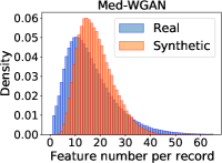
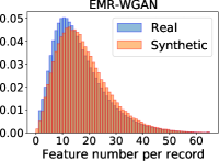
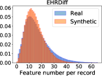
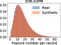
Figure 4: Density comparison of per-record feature number between synthetic data and real data $\mathcal{D}_{1}$. The number of features per record is computed summing the ICD codes present in each sample. The number of bins is 65 and the range of feature number values is (0, 65).

5.3 Evaluation Metrics

Dimension-wise Prevalence We compute dimension-wise prevalence by taking the mean of the data in each dimension. Dimension-wise prevalence is a vector which has the same dimension as the input data. Dimension-wise prevalence captures the marginal feature distribution of the data. We compute the Spearman correlation between prevalence in the synthetic data and prevalence in the real data.

Correlation Matrix Distance (CMD) measures the difference between the covariance matrix of the synthetic data and the covariance matrix of real data. We first compute the empirical covariance matrices of the synthetic data and real data respectively and take the difference between these two matrices. Then we calculate the Frobenius norm of the difference matrix as distributional distance.

Maximum Mean Discrepancy (MMD) is one of most common metrics to measure the difference between two distributions in distributional space. We compute the MMD for a set of synthetic data and a set of real test data. We employ a mixture of kernel-based methods (Li et al., 2017) to estimate MMD to improve its robustness. The detailed formula is given in Eq.(6) in Appendix A.4.

Downstream Prediction To evaluate the utility of the generated synthetic data, we evaluate the accuracy of classifiers trained to predict the diseases of interest mentioned above using synthetic data. We train the classifiers to predict the ICD code that corresponds to the disease of interest using all other available ICD codes as features. We train the classification model using synthetic data and evaluate its performance on real test data. We adopt the state-of-the-art robust classification model for tabular data given in (Ke et al., 2017). The most reliable classification model is one trained on real data; we use this as a benchmark to represent an upper bound for classification accuracy.

Membership Inference Risk (MIR) evaluates the risk that an attacker can infer the real samples used for training the generative model given generated synthetic EHR data or the model parameters. We consider the attack model MIR (Duan et al., 2023) proposed for diffusion models with continuous data. Following Yan et al. (2022), we evaluate MIR on discrete data. For each EHR in this set of real training and evaluation data, we calculate the minimum L2 distance with respect to the synthetic EHR data. The real EHR whose distance is smaller than a preset threshold is predicted as the training EHR. We report the prediction F1 score to demonstrate the performance of each model under membership inference risk.

5.4 Experiment Results

Table 1: Synthetic data utility. Disease prediction from ICD codes using the real dataset $\mathcal{D}_{1}$. AUPRC and AUROC are reported. AUPR and AUC in table are short for AUPRC and AUROC respectively. We use synthetic data of size 160K to train the classifier and 200K real test data samples to evaluate the different methods. 80% of the test data are bootstrapped 50 times to compute 95% confidence intervals (CI). The values of CI for all cases are between 0.001 and 0.003 and therefore not shown in table, provided on Appendix B.

	Diabetes	Asthma	COPD	CKD	HTN-Heart	Osteoarthritis
	AUPR AUC	AUPR AUC	AUPR AUC	AUPR AUC	AUPR AUC	AUPR AUC
Real Data	0.702  0.808	0.288  0.759	0.675  0.867	0.806  0.913	0.253  0.832	0.296  0.789
Med-WGAN	0.628  0.757	0.149  0.595	0.578  0.806	0.722  0.873	0.114  0.625	0.192  0.661
EMR-WGAN	0.656  0.770	0.193  0.642	0.603  0.815	0.753  0.885	0.151  0.686	0.219  0.689
EHRDiff	0.670  0.780	0.232  0.722	0.642  0.856	0.782  0.902	0.150  0.714	0.245  0.759
EHR-D3PM	0.693  0.801	0.263  0.748	0.655  0.860	0.796  0.908	0.229  0.821	0.278  0.782

Fidelity

We first evaluate the learnt distributions using the MIMIC-III dataset in Fig. 1, dataset $\mathcal{D}_{1}$ in Fig. 3 and dataset $\mathcal{D}_{2}$ in Fig. 7 in Appendix B.1. We compare prevalence in synthetic data with prevalence in real data for each dimension. In Fig. 1, Fig. 3 and Fig. 7, we can see that the prevalence for our method EHR-D3PM aligns best with the real data. EHR-D3PM consistently has the highest Spearman correlation. We further observe that Med-WGAN, EMR-WGAN and EHRDiff fail to provide an unbiased estimation of the distribution in the low prevalence regime, which corresponds to rare conditions. This failure is mild when the dataset has dense features, as shown in Fig. 7 of $\mathcal{D}_{2}$, but is obvious when the dataset has sparse features, as shown in Fig. 3 of $\mathcal{D}_{1}$.

Next we compare our method in terms of feature number per record, which is calculated by summing the ICD codes in each sample, using the MIMIC dataset-III in Fig. 2, dataset $\mathcal{D}_{1}$ in Fig. 4 and dataset $\mathcal{D}_{2}$ in Fig. 8 in Appendix B.1. We compare feature numbers for synthetic data with that of real data. As we see in Fig. 2, Fig. 4 and Fig. 8, Med-WGAN, EMR-WGAN and EHRDiff demonstrate poor performance in estimating the mode or the tail of the density. When the datasets are large, our method tends to provide a perfect estimation of the feature number for the real data.

Finally we compare our method in terms of the CMD and MMD metrics. Tabel 2 shows that our EHR-D3PM significantly outperforms all baselines, particularly with the larger datasets $\mathcal{D}_{1}$ and $\mathcal{D}_{2}$. This indicates our method can learn much better pairwise correlations between different feature dimensions. Table 2 also shows that the distribution of synthetic data generated by our method has the least discrepancy with real data distribution on all three datasets.

Table 2: Additional fidelity metrics (CMD and MMD) and privacy metric (MIR) on MIMIC, dataset $\mathcal{D}_{1}$ and dataset $\mathcal{D}_{2}$. 95% confidence intervals are provided in Table 11 and Table 11 on Appendix B.

	Fidelity CMD($\downarrow$)	Fidelity MMD($\downarrow$)	Privacy MIR($\downarrow$)
	MIMIC         $\mathcal{D}_{1}$          $\mathcal{D}_{2}$	MIMIC       $\mathcal{D}_{1}$          $\mathcal{D}_{2}$	MIMIC       $\mathcal{D}_{1}$          $\mathcal{D}_{2}$
Med-WGAN	27.540    18.107    28.942	0.078      0.075      0.086	0.440      0.339      0.398
EMR-WGAN	26.658    11.869    21.438	0.053      0.018      0.024	0.456      0.358      0.415
EHRDiff	25.447    23.208    18.941	0.009      0.023      0.046	0.445      0.353      0.421
EHR-D3PM	21.128     7.692    10.255	0.003      0.012      0.019	0.432      0.344      0.406

Utility We now apply our method to disease classification downstream tasks. Since MIMIC-III contains a much smaller patient population than the private datasets, which may not provide a valid test data benchmark for disease classification, we focus on the private datasets $\mathcal{D}_{1}$ and $\mathcal{D}_{2}.$ In Table 4, we observe that the prevalence of most diseases is low in datasets $\mathcal{D}_{1}$ and $\mathcal{D}_{2}.$ The training and test data set sizes are 160K and 200K. From Table 1, the average increase in AUPRC and AUROC over the strongest baseline (EHRDiff) is 3.90% and 2.57% respectively for dataset $\mathcal{D}_{1}$. From Table 5, the average increase in AUPRC and AUROC over the strongest baseline (EHRDiff) is 3.22% and 3.12% respectively for dataset $\mathcal{D}_{2}.$

Privacy We evaluate the membership inference risk (MIR) of our method and other baselines on each dataset. Table 2 shows the MIRs of our method is lower than other baslines across all datasets, indicating our method has mild vulnerability to privacy risk compared to existing baselines. As there is a trade-off between privacy and fidelity, incorporating differential privacy to further reduce the privacy risk in diffusion models is an interesting direction, which is largely unexplored in discrete diffusion models.

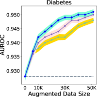
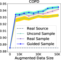
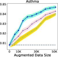
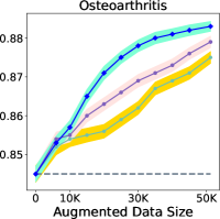
Figure 5: Synthetic data augmentation for disease classifications from ICD codes based on dataset $\mathcal{D}_{2}$. The size of the real source data for training the LGBM classifier is 5000, as indicated by the dashed purple line. We augment the source training data with synthetic data to train the LGBM classifier. "Uncond Samples" stands for the synthetic data generated by our unconditional sampler. Guided samples are synthetic data generated by our proposed guided sampler for each disease. To minimize noise from evaluation, we adopt 200K real test data to evaluate all experiments and report test AUROC for comparison. 80% of the test data are bootstrapped 50 times to compute 95% CI, which is added in shaded region.

5.5 Guided Generation

In this section, we apply our guided sampling method to generate conditional samples for different disease conditions. For each condition, we apply our guided sampler and generate a set of synthetic data. Table 3 lists the prevalence of four diseases in the real data $\mathcal{D}_{2}$. As we can see, the prevalence of diabetes, COPD, Asthma and Osteoarthritis are very low. The prevalence of samples generated by our unconditional sampling method matches the prevalence of each in the real datam, while synthetic samples generated by our guided sampler demonstrate a more balanced ratio.

Table 3: Prevalence of diseases in different sample groups. "Real" means real dataset $\mathcal{D}_{2}$. "Uncond" is short for samples generated by our unconditional method. "Guided" stands for samples generated by our guided sampler.

	Diabetes	COPD	Asthma	Osteoarthritis
Real	0.068	0.017	0.079	0.034
Uncond	0.069	0.015	0.073	0.036
Guided	0.202	0.042	0.161	0.137

In the following, we utilize synthetic samples to augment the training dataset when training downstream disease classifiers. The size of the real source data for training classifiers is 5000. We augment the original training data with data from three different groups: real data, synthetic data generated by our unconditional sampling method and our guided sampling method. We report AUROC in Fig. 5 and AUPRC in Fig. 9 in AppendixB.2 to evaluate accuracy. We can see that classifiers trained with synthetic data augmentation always improve the vanilla baseline (classifier trained with the original source data). We also observe that the data augmentation by guided sampling consistently outperform the data augmentation by unconditional sampling. It is interesting to observe that the data augmentation by guided sampling has consistently higher AUROC than real data augmentation. We observe this to be because the synthetic samples generated by guided sampling contain richer information in cases of diseases of low prevalence.

6 Conclusion and Future Work

In this paper, we introduced a novel generative model for synthesizing realistic EHRs EHR-D3PM. Leveraging the latest advancements in discrete diffusion models, EHR-D3PM overcomes the challenges of GAN-based approaches and effectively generates high-quality tabular medical data. Compared with other diffusion-based approaches, EHR-D3PM enables high-quality conditional generation. Our experiment demonstrates that EHR-D3PM not only achieves state-of-the-art performance in fidelity, utility, and privacy metrics but also significantly improves downstream task performance through data augmentation. Further investigations of the vulnerability of diffusion-based generative models in EHR generation, particularly to Membership Inference Attacks (MIAs) (Shokri et al., 2017), is a promising future direction as well as providing formal privacy guarantees, e.g., by incorporating differential privacy, which is largely unexplored in diffusion-based models for discrete data.

Appendix A Experiment Details.

In the following Table 4, we present a concise summary of various diseases along with their corresponding International Classification of Diseases, Ninth Revision (ICD 9) codes. $\mathcal{D}_{1},\mathcal{D}_{2}$ represents the real dataset 1 and real dataset 2, respectively. This table includes common conditions such as Type II Diabetes (T2D), Chronic Kidney Disease (CKD), Chronic Obstructive Pulmonary Disease (COPD), Asthma, Hypertension and Osteoarthritis. Each disease is associated with specific ICD 9 codes that are used for clinical classification and diagnosis purposes. In this paper, we are interested in the diseases listed in Table 4.

Table 4: List of Diseases and Corresponding ICD 9 Codes.

Disease	ICD 9 Code	MIMIC	Dataset $\mathcal{D}_{1}$	Dataset $\mathcal{D}_{2}$
Diabetes	250.*	0.214	0.261	0.068
Chronic Kidney Disease (CKD)	585.1–9	0.106	0.119	0.015
Chronic Obstructive Pulmonary Disease (COPD)	496	0.069	0.136	0.017
Asthma	493.20–22	0.051	0.085	0.079
Hypertension (HTN-Heart)	402.*	0.001	0.028	0.006
Osteoarthritis	715.96	0.0197	0.061	0.034

A.1 Dataset Details

MIMIC Dataset

The MIMIC III dataset includes a patient population of 46,520. There are 651,047 positive codes within 64,314 hospital admission records (HADM IDs). We have implemented an 80/20 split for training and testing purposes. Specifically, this allocates 12,862 records for testing and the remaining 51,451 for training. The histograms in Fig. 2 indicate the density distribution of feature number per record. The dimension is $N=1042.$

Dataset $\mathcal{D}_{1}$

The first dataset, denoted by $\mathcal{D}_{1}$, includes a patient population of size 1,670,347. We split the whole dataset into 100K for validation, 2000K for testing and the rest 1,370, 347 for training. The number of codes per patient is relatively small, as indicated by the histogram of feature number per record in Fig. 4. The dimension is $N=993.$

Dataset $\mathcal{D}_{2}$

The second dataset, denoted by $\mathcal{D}_{2}$, includes a patient population of size 1,859,536. We split the whole dataset into 100K for validation, 2000K for testing and the rest 1,559,536 for training. The number of codes per patient is relatively large, as indicated by the histogram of feature number per record in Fig. 8. Although, dataset $\mathcal{D}_{2}$ has relatively denser feature, the prevalence of six chronic diseases we are interested in is pretty low. The dimension is $N=993.$

A.2 Model Architecture Detail

The denoise model in this paper has a uniform architecture, illustrated in Fig. 6. The architecture we propose is tailored for tabular EHRs as it is non-sequential data. While the architecture proposed in multinomial diffusion Hoogeboom et al. (2021b) is designed for sequential data, where neighboring dimensions have semantic correlation. The tabular EHR datasets in our paper don’t have such property. Therefore, we propose a novel transformer-based model for tabular EHRs. One bottleneck of transformer models is that the computational complexity of the attention module is quadratic to the dimension of input data. We adopt an efficient block based on  Wang et al. (2020), whose attention operation has linear complexity with respect to the dimension of input data.

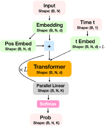
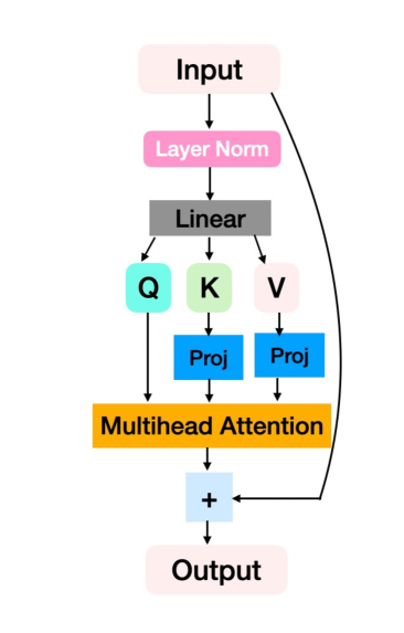
(a) Denoise Model	(b) Transformer Block

Figure 6: Architecture of our denoise model. (b) provides the detail of transformer block which has linear complexity with respect to the dimension of input. Axial positional embedding is employed to encode the positional information. We employ sinusoidal positional embedding to time $t$ to the time embedding and then use a two-layer MLPs to map the time embedding into hidden state. In the first layer of the two-layer MLP, we use Softplus activation function. We apply L times of such two-layer MLP to get the hidden state of time embedding to yield the input of each transformer block, as indicated in (a). Positional embedding is added to the embedding of discrete inputs. The input has dimension N and B means the batch size. For notation simplicity, we use all dimension of tabular data has K categories. We use one-hot representation and therefore, the output of the denoise model has shape (B, N, K). The shape of intermediate layers is provided in (a). In (b), "Proj" denotes the projection operation proposed in Linformer Wang et al. (2020), which induces the linear complexity of the attention module with respect to the input dimension $N$. The projection dimension is set as the default value 128 for all experiments in this paper.

A.3 Hyper-parameters

Hyper-parameters on MIMIC dataset

Since the MIMIC III dataset is relatively small, we use a relative small model to train our EHR-D3PM to avoid overfitting to the training data. The hidden dimension 256. The number of multi-attention heads is 8. The number of transformer layers is 5. The number of diffusion steps is 500.

In the optimization phrase, we adopt adamW optimizer, and the weight decay in adamW is 1.e-5. The learning rate is 1e-4 and batch size is 256. The beta for expentialLR in learning rate schedule is 0.99. The number of training epochs is 100. It takes less than three hours to finish training this model on A6000 with 48G memory.

Hyper-parameters on datasets $\mathcal{D}_{1}$ and $\mathcal{D}_{2}$

The denoise model for datasets $\mathcal{D}_{1}$ and $\mathcal{D}_{2}$ are the same. As datasets $\mathcal{D}_{1}$ and $\mathcal{D}_{2}$ are large, we use a relatively large model. The number of multi-attention heads is 8. The hidden dimension is 512. The number of transformer layers $L$ is 8. The number of diffusion steps is 500.

The optimization parameters for both datasets $\mathcal{D}_{1}$ and $\mathcal{D}_{2}$ are also the same. In the optimization phrase, we adopt adamW optimizer. The learning rate is 1e-4 and batch size is 512. The weight decay in adamW is 1.e-5. The beta for expentialLR in learning rate schdule is 0.99. The number of training epochs is 40. It takes one and half day to train one model on A100 with 80G memory.

Hyper-parameters of baseline EHRDiff

To have a fair comparison with diffusion baseline EHRDiff, we use the same hyper parameters as our proposed diffusion model on all three datasets. The number of diffusion steps in EHRDiff is also 500 and the number of layers in EHRDiff is also 5. The other hyper parameters use the default values in the github implementation of EHRDiff.

A.4 Evaluation Metrics

MMD

The empirical MMD between two distributions P and Q is approximated by

$$\mathrm{MMD}(P,Q)=\frac{1}{m}\sum_{\gamma=1}^{m}\widehat{\mathrm{MMD}}_{k_{\gamma}}(P,Q),$$ (6)

where $k_{\gamma}$ is a kernel function; m is number of kernels; $\widehat{\mathrm{MMD}}_{k_{\gamma}}(P,Q)$ is estimated by samples $\{\mathbf{x}_{i}\}_{i=1}^{n}\sim P$ and $\{\mathbf{x}^{\prime}_{i}\}_{i=1}^{n}\sim Q$ as follows,

$$\widehat{\mathrm{MMD}}_{k_{\gamma}}(P,Q)=\frac{1}{n(n-1)}[\sum_{i\neq j}k_{\gamma}(\mathbf{x}_{i},\mathbf{x}_{j})+\sum_{i\neq j}k_{\gamma}(\mathbf{x}^{\prime}_{i},\mathbf{x}^{\prime}_{j})]-\frac{1}{n^{2}}\sum_{i,j}k_{\gamma}(\mathbf{x}_{i},\mathbf{x}^{\prime}_{j}).$$

In our evaluation, we use Gaussian RBF kernel $k_{\gamma}$,

$$k_{\gamma}(\mathbf{x},\mathbf{x}^{\prime})=\mathrm{exp}(-\frac{\|\mathbf{x}-\mathbf{x}^{\prime}\|^{2}}{2h^{2}_{\gamma}})$$

with bandwidth $h_{\gamma}=\mathrm{Avg}*2^{(\gamma-m/2)}$, where $\mathrm{Avg}$ is the average of pairwise L2 distance between all samples. We choose $m=5$ and thus $\gamma\in\{1,2,3,4,5\}$.

A.5 Hyper-parameters of Classifier Models on Downstream Tasks

For the downstream tasks, we used a light gradient boosting decision tree model (LGBM) (Ke et al., 2017) as it had uniformly robust prediction performance on all downstream tasks. In all experiments, we set the hyper-parameters of LGBM as follows: $\mathrm{n\_estimators}=1000$, $\mathrm{learning\_rate}=0.05$ $\mathrm{max\_depth}=10$, $\mathrm{reg\_alpha}=0.5$, $\mathrm{reg\_lambda}=0.5$, $\mathrm{scale\_pos\_weight}=1$, $\mathrm{min\_data\_in\_bin}=128.$ We also experiment with various sets of hyper parameters which will induce the same conclusion we have in this paper.

Appendix B Additional Experiments

Due to space limit, we leave a bunch of experiment results on appendix.

B.1 Additional experiments on unconditional generation

Fidelity

Fig. 7 provides additional comparison of marginal distribution matching on dataset $\mathcal{D}_{2}$. Since dataset $\mathcal{D}_{2}$ has relatively denser features, the performance of baselines in low prevalence regime is less severe than that of baselines on dataset $\mathcal{D}_{1}$. From the Spearman correlation in low prevalence regime, we can still see that our method significantly outperform baselines. Based on results in Fig. 1, Fig. 3 and Fig. 7, we consistently observe synthetic data by EHRDiff fails to capture the information in low prevalence regime. One reason we articulate is that the foundation of EHRDiff is designed for continuous distribution and cannot be readily applied to the generation of discrete data particularly on data of low prevalence regime. From Fig. 8, we can see that the histogram of feature number per record on synthetic data by our method provides a perfect matching to that of real data.

Utility

We also apply our methods to downstream prediction tasks on dataset $\mathcal{D}_{2}$, where the prevalence of six chronic diseases is much lower. From Fig 5, we can see that the accuracy of our prediction is still close to the prediction of classifier models trained on real data, which is the classifier baseline. While other baselines have a much larger performance gap when compared with the ideal classifier. Particularly on rare diseases such as hypertension heart, the classifier trained on synthetic data by our model has 8% absolute improvement in AUPRC and AUROC over the strongest baseline on both $\mathcal{D}_{1}$ and $\mathcal{D}_{2}$. From the confidence intervals provided in Table 7, 6, 8 and 9, we confirm that such improvement over the baselines are statistically significant.

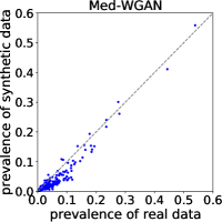
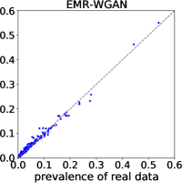
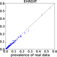
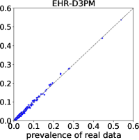
(a) Spearm corr = 0.96	(b) Spearm corr = 0.99	(c) Spearm corr = 0.95	(d) Spearm corr = 0.99
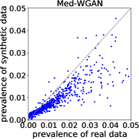
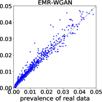
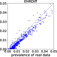
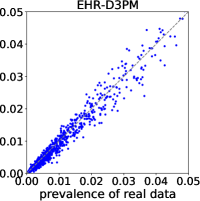
(e) Spearm corr = 0.95	(f) Spearm corr = 0.98	(g) Spearm corr = 0.94	(h) Spearm corr = 0.98

Figure 7: Comparison between prevalence of synthetic data and prevalence of real dataset $\mathcal{D}_{2}$. It measures accuracy of the marginal distribution for each ICD code on synthetic samples. The second row represents the prevalence of the first row in low data regime. The prevalence is computed on 200K samples. The dash diagonal lines represent the perfect matching of code prevalence between synthetic data and real EHR data. The Pearson correlations for four methods are all greater than 0.99 and will not be used as a metric to evaluate different methods.

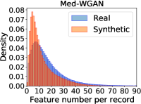
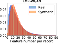
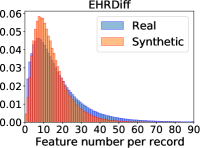
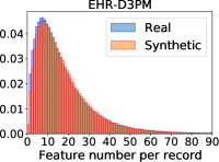
Figure 8: Density comparison of per-record feature number between synthetic data and real dataset $\mathcal{D}_{2}$. The number of feature per record is computed by sum of ICD codes on each sample. Number of bins is 90 and the range of feature number values is (0, 90).

Table 5: Synthetic data utility. Disease prediction from ICD codes on real dataset $\mathcal{D}_{2}$. AUPRC and AUROC are reported. AUPR and AUC in table are short for AUPRC and AUROC respectively. We use synthetic data of 160K to train the classifier and 200K real test data to evaluate different methods. 80% of test data are bootstrapped 50 times to compute for 95% confidence interval (CI). The values of CI for all cases are between 0.001 and 0.011.

	T2D	Asthma	COPD	CKD	HTN-Heart	Osteoarthritis
	AUPR AUC	AUPR AUC	AUPR AUC	AUPR AUC	AUPR AUC	AUPR AUC
Real data	0.834  0.955	0.581  0.853	0.622  0.951	0.733  0.944	0.278  0.926	0.373  0.893
Med-WGAN	0.725  0.924	0.496  0.819	0.203  0.853	0.166  0.835	0.008  0.500	0.223  0.820
EMR-WGAN	0.734  0.918	0.431  0.747	0.402  0.888	0.628  0.907	0.134  0.844	0.210  0.753
EHRDiff	0.807  0.950	0.549  0.843	0.548  0.936	0.690  0.916	0.141  0.822	0.319  0.875
EHR-D3PM	0.821  0.952	0.572  0.853	0.607  0.947	0.714  0.944	0.226  0.911	0.348  0.889

B.2 Additional experiments on guided generation

We provide additional experiment results on guided generation. We augment the real data with synthetic data generated by our sampling method and train a downstream classifier. We measure the performance of all classifiers on real test data. From Fig. 9 and Fig. 5, we see that the classifier trained on augmented training data with synthetic data, either by our unconditional sampling method or by our guided sampling method, consistently outperforms the classifier trained with original source data (vanilla baseline). In all cases, the relative increase of AUPRC over vanilla baseline is more than 3%; in the classification of COPD, the relative improvement over the vanilla baseline is more than 30%. This clearly indicates that our method can be applied to augment the training data of downstream classification tasks when the real dataset is scarce. More importantly, the data augmentation by guided sampler consistently outperforms the data augmentation with unconditional sampler. We observe this to be because the synthetic samples generated by guided sampling contain richer information in diseases of low prevalence. A most balanced training data with positive label will enhance the performance of classifiers and reduce the risk of over fitting to negative class.

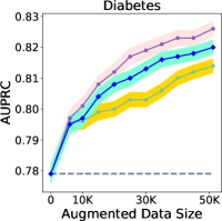
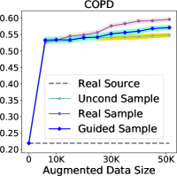
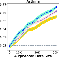
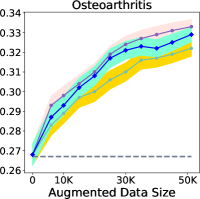
Figure 9: Synthetic data augmentation for disease classification from ICD codes based on dataset $\mathcal{D}_{2}$. The size of real source data for training LGBM classifier is 5000, as indicated in dashed line. We augment the original source training data with synthetic data to train LGBM classifier. "Uncond Samples" stands for the synthetic data generated by our unconditional sampler. Guided samples are synthetic data generated by our proposed guided sampler for each disease. To minimize noise from evaluation, we adopt 200K real test data to evaluate all experiments and report test AUROC for comparison. 80% of the test data are bootstrapped 50 times to compute 95% confidence intervals (CI), which is added as shaded region.

Table 6: Synthetic data utility. Disease prediction from ICD codes on real data $\mathcal{D}_{1}$. AUPRC is reported. We use synthetic data of 160K to train the classifier and 200K real test data to evaluate different methods. 80% of test data are bootstrapped for 50 times to compute for 95% confidence interval.

	T2D	Asthma	COPD	CKD	HTN-Heart	Osteoarthritis
Real Data	0.702 $\pm$ 0.002	0.288 $\pm$ 0.004	0.675 $\pm$ 0.002	0.806 $\pm$ 0.002	0.253 $\pm$ 0.003	0.296 $\pm$ 0.003
Med-WGAN	0.628 $\pm$ 0.002	0.149 $\pm$ 0.002	0.578 $\pm$ 0.002	0.722 $\pm$ 0.002	0.114 $\pm$ 0.001	0.192 $\pm$ 0.003
EMR-WGAN	0.656 $\pm$ 0.002	0.193 $\pm$ 0.002	0.603 $\pm$ 0.002	0.753 $\pm$ 0.002	0.151 $\pm$ 0.003	0.219 $\pm$ 0.003
EHRDiff	0.670 $\pm$ 0.002	0.232 $\pm$ 0.003	0.642 $\pm$ 0.002	0.782 $\pm$ 0.002	0.150 $\pm$ 0.002	0.245 $\pm$ 0.003
EHR-D3PM	0.693 $\pm$ 0.002	0.263 $\pm$ 0.003	0.655 $\pm$ 0.002	0.796 $\pm$ 0.002	0.229 $\pm$ 0.003	0.278 $\pm$ 0.003

Table 7: Synthetic data utility. Disease prediction from ICD codes on real dataset $\mathcal{D}_{1}$. AUROC is reported. We use synthetic data of 160K to train the classifier and 200K real test data to evaluate different methods. 80% of test data are bootstrapped for 50 times to compute 95% confidence interval.

	T2D	Asthma	COPD	CKD	HTN-Heart	Osteoarthritis
Real data	0.808 $\pm$ 0.001	0.759 $\pm$ 0.002	0.867 $\pm$ 0.001	0.913 $\pm$ 0.001	0.832 $\pm$ 0.001	0.789 $\pm$ 0.001
Med-WGAN	0.757 $\pm$ 0.001	0.595 $\pm$ 0.002	0.806 $\pm$ 0.001	0.873 $\pm$ 0.001	0.625 $\pm$ 0.002	0.661 $\pm$ 0.002
EMR-WGAN	0.770 $\pm$ 0.001	0.642 $\pm$ 0.002	0.815 $\pm$ 0.001	0.885 $\pm$ 0.001	0.686 $\pm$ 0.002	0.689 $\pm$ 0.002
EHRDiff	0.789 $\pm$ 0.001	0.722 $\pm$ 0.002	0.856 $\pm$ 0.001	0.902 $\pm$ 0.001	0.714 $\pm$ 0.002	0.759 $\pm$ 0.002
EHR-D3PM	0.801 $\pm$ 0.001	0.748 $\pm$ 0.002	0.860 $\pm$ 0.001	0.908 $\pm$ 0.001	0.821 $\pm$ 0.002	0.782 $\pm$ 0.002

Table 8: Synthetic data utility. Disease prediction from ICD codes on real data $\mathcal{D}_{2}$. AUPRC is reported. We use synthetic data of 160K to train the classifier and 200K real test data to evaluate different methods. 80% of test data are bootstrapped 50 times to compute 95% confidence interval.

	T2D	Asthma	COPD	CKD	HTN-Heart	Osteoarthritis
Real data	0.834 $\pm$ 0.002	0.581 $\pm$ 0.005	0.622 $\pm$ 0.009	0.733 $\pm$ 0.006	0.278 $\pm$ 0.011	0.373 $\pm$ 0.005
Med-WGAN	0.725 $\pm$0.003	0.496 $\pm$ 0.005	0.203 $\pm$ 0.007	0.166 $\pm$ 0.005	0.008 $\pm$ 0.001	0.223 $\pm$ 0.004
EMR-WGAN	0.734 $\pm$0.003	0.431 $\pm$ 0.004	0.402 $\pm$ 0.007	0.628 $\pm$ 0.009	0.134 $\pm$ 0.008	0.210 $\pm$ 0.004
EHRDiff	0.807 $\pm$0.003	0.549 $\pm$ 0.004	0.548 $\pm$ 0.007	0.690 $\pm$ 0.008	0.141 $\pm$ 0.009	0.319 $\pm$ 0.005
EHR-D3PM	0.821 $\pm$0.002	0.572 $\pm$ 0.004	0.607 $\pm$ 0.007	0.714 $\pm$ 0.007	0.226 $\pm$ 0.008	0.348 $\pm$ 0.006

Table 9: Synthetic data utility. Disease prediction from ICD codes on real data $\mathcal{D}_{2}$. AUROC is reported. We use synthetic data of 160K to train the classifier and 200K real test data to evaluate different methods. 80% of test data are bootstrapped 50 times to compute 95% confidence interval.

	T2D	Asthma	COPD	CKD	HTN-Heart	Osteoarthritis
Real data	0.955 $\pm$ 0.001	0.853 $\pm$ 0.002	0.951 $\pm$ 0.002	0.944 $\pm$ 0.002	0.926 $\pm$ 0.003	0.893 $\pm$ 0.002
Med-WGAN	0.924 $\pm$ 0.001	0.819 $\pm$ 0.002	0.853 $\pm$ 0.003	0.835 $\pm$ 0.004	0.5 $\pm$ 0.001	0.820 $\pm$ 0.003
EMR-WGAN	0.918 $\pm$ 0.001	0.747 $\pm$ 0.002	0.888 $\pm$ 0.003	0.907 $\pm$ 0.003	0.844 $\pm$ 0.005	0.753 $\pm$ 0.003
EHRDiff	0.950 $\pm$ 0.001	0.843 $\pm$ 0.002	0.936 $\pm$ 0.002	0.916 $\pm$ 0.004	0.822 $\pm$ 0.006	0.875 $\pm$ 0.002
EHR-D3PM	0.952 $\pm$ 0.001	0.853 $\pm$ 0.002	0.947 $\pm$ 0.002	0.944 $\pm$ 0.002	0.911 $\pm$ 0.004	0.889 $\pm$ 0.002

Table 10: Fidelity metrics (CMD and MMD) on MIMIC, dataset $\mathcal{D}_{1}$ and dataset $\mathcal{D}_{2}$. 95% confidence intervals are provides.

	CMD($\downarrow$)	MMD($\downarrow$)
	MIMIC              $\mathcal{D}_{1}$               $\mathcal{D}_{2}$	MIMIC             $\mathcal{D}_{1}$              $\mathcal{D}_{2}$
Med-WGAN	27.540$\pm$0.628  18.107$\pm$0.128  28.942$\pm$0.196	0.078$\pm$0.0089 0.075$\pm$0.011 0.086$\pm$0.013
EMR-WGAN	26.658$\pm$0.638  11.869$\pm$0.108  21.438$\pm$0.146	0.053$\pm$0.0054 0.018$\pm$0.003 0.024$\pm$0.004
EHRDiff	25.447$\pm$0.488  23.208$\pm$0.088 18.941$\pm$0.092	0.009$\pm$0.0013 0.023$\pm$0.003 0.046$\pm$0.005
EHR-D3PM	21.128$\pm$0.393  7.692$\pm$0.028  10.255$\pm$0.037	0.003$\pm$0.0004 0.012$\pm$0.001 0.019$\pm$0.002

Table 11: Additional fidelity metric (MCAD) on MIMIC, dataset $\mathcal{D}_{1}$ and dataset $\mathcal{D}_{2}$.

	MCAD($\downarrow$)
	MIMIC                     $\mathcal{D}_{1}$                      $\mathcal{D}_{2}$
Med-WGAN	0.1896$\pm$0.0024       0.1871$\pm$0.0016      0.1944$\pm$0.0017
EMR-WGAN	0.1546$\pm$0.0167       0.1625$\pm$0.0013      0.1572$\pm$0.0015
EHRDiff	0.1439$\pm$0.0015      0.1687$\pm$0.0014      0.1764$\pm$0.0016
EHR-D3PM	0.1013$\pm$0.0010      0.0873$\pm$0.0007      0.1081$\pm$0.0009

Table 12: Privacy metric (MIR) on MIMIC, dataset $\mathcal{D}_{1}$ and dataset $\mathcal{D}_{2}$.

	Privacy MIR($\downarrow$)
	MIMIC       $\mathcal{D}_{1}$          $\mathcal{D}_{2}$
Med-WGAN	0.440$\pm$0.0034      0.339$\pm$0.0018      0.398$\pm$0.0019
EMR-WGAN	0.456$\pm$0.0035      0.358$\pm$0.0017      0.415$\pm$0.0020
EHRDiff	0.445$\pm$0.0034      0.353$\pm$0.0015      0.421$\pm$0.0019
EHR-D3PM	0.432$\pm$0.0034      0.344$\pm$0.0016      0.406$\pm$0.0018

Appendix C Additional Details of EHR-D3PM

If $\mathbf{x}$ is a continuous variable, the most common way to sample from the posterior $p_{\bm{\theta}}(\mathbf{x}|\mathbf{c})\propto p_{\bm{\theta}}(\mathbf{x})\cdot p(\mathbf{c}|\mathbf{x})$ is using the following Langevin dynamics,

$$\mathbf{x}^{(k+1)}\leftarrow\mathbf{x}^{(k)}+\eta\tau_{1}\nabla\log p(\mathbf{c}|\mathbf{x})+\eta\nabla\log p_{\bm{\theta}}(\mathbf{x})+\sqrt{\eta\tau_{2}}\bm{\epsilon},$$ (7)

where $\bm{\epsilon}\sim\mathcal{N}(0,\mathbf{I})$. (7) has been applied in image (Dhariwal and Nichol, 2021) and recently be applied to EHR generation with Gaussian diffusion (He et al., 2023). In practice, $\tau_{2}$ is always chosen to be zero in practice, and we will generally use $V(\mathbf{x}):=\log(p(c|\mathbf{x}))$ to replace the likelihood that we want to maximize in (7).

For discrete data, (7) is intractable since we can’t get the gradient backpropagation via $\nabla\log p_{\bm{\theta}}(\mathbf{x})$. In addition, (7) can’t guarantee that $\mathbf{x}^{(k+1)}$ lies in the category $\{1,\ldots,K\}$ after update. Therefore, we need to do Langevin updates on the latent space $\mathbf{z}_{L,t}$

$$\mathbf{y}^{(k+1)}\leftarrow\mathbf{y}^{(k)}-\eta\nabla_{\mathbf{y}^{(k)}}[\mathcal{D}_{\mathrm{KL}}(\mathbf{y}^{(k)})-V_{\bm{\theta}}(\mathbf{y}^{(k)})]+\sqrt{2\eta\tau}\bm{\epsilon},$$

where $\mathbf{y}^{(k)}$ is the modification of $\mathbf{z}_{L,t}$, and $\mathcal{D}_{\mathrm{KL}}(\mathbf{y}^{(k)})=\lambda\mathrm{KL}(p_{\theta}(\widehat{\mathbf{x}}_{0}|\mathbf{y}^{(k)})||p_{\theta}(\widehat{\mathbf{x}}_{0}|\mathbf{y}^{(0)}))$ is the $\mathrm{KL}$ divergence for regularization of the guided Markov transition. The gradient of the KL term plays a similar role as $\nabla p_{\bm{\theta}}(\mathbf{x})$ in (7). It will be interesting to leverage deterministic updates Liu and Wang (2016); Han and Liu (2018) to accelerate this process.

Example: Suppose that the context $c$ is to generate a EHR $\mathbf{x}$ such that $\mathbf{x}$ has diabete disease, i.e., the $k$-th token of $\mathbf{x}$ equals $[1,0]$, where $k=156$ for MIMIC data set. Then we have $p(c|\widehat{\mathbf{x}}_{0})=1$ if $k$-th token of $\mathbf{x}$ equals $[1,0]$ and $p(c|\widehat{\mathbf{x}}_{0})=0$ otherwise. In addition $p_{\bm{\theta}}(\widehat{\mathbf{x}}_{0}|\mathbf{y}^{(k)})$ is the $k$-th position output of softmax layer when input $\mathbf{y}^{(k)}$. Then we can compute the energy function as follows,

$$V_{\bm{\theta}}(\mathbf{y}^{(k)})=\log(p(\mathbf{c}|\mathbf{y}^{(k)}))=\log\bigg{(}\sum_{\widehat{\mathbf{x}}_{0}}p_{\bm{\theta}}(\widehat{\mathbf{x}}_{0}|\mathbf{y}^{(k)})p(\mathbf{c}|\widehat{\mathbf{x}}_{0})\bigg{)}.$$

In all experiments of guided generation, the number of Langevin update steps is 10, $\eta=0.1$ and $\lambda=0.01.$

References

- Austin et al. (2021) Austin, J., Johnson, D. D., Ho, J., Tarlow, D. and Van Den Berg, R. (2021). Structured denoising diffusion models in discrete state-spaces. Advances in Neural Information Processing Systems 34 17981–17993.
- Baowaly et al. (2018) Baowaly, M. K., Lin, C.-C., Liu, C.-L. and Chen, K.-T. (2018). Synthesizing electronic health records using improved generative adversarial networks. Journal of the American Medical Informatics Association 26 228–241.
- Bartlett et al. (2019) Bartlett, V. L., Dhruva, S. S., Shah, N. D., Ryan, P. and Ross, J. S. (2019). Feasibility of using real-world data to replicate clinical trial evidence. JAMA network open 2 e1912869–e1912869.
- Biswal et al. (2021) Biswal, S., Ghosh, S., Duke, J., Malin, B., Stewart, W., Xiao, C. and Sun, J. (2021). Eva: Generating longitudinal electronic health records using conditional variational autoencoders. In Machine Learning for Healthcare Conference. PMLR.
- Biswal et al. (2020) Biswal, S., Ghosh, S. S., Duke, J. D., Malin, B. A., Stewart, W. F. and Sun, J. (2020). Eva: Generating longitudinal electronic health records using conditional variational autoencoders. ArXiv abs/2012.10020.
- Buczak et al. (2010) Buczak, A. L., Babin, S. and Moniz, L. J. (2010). Data-driven approach for creating synthetic electronic medical records. BMC Medical Informatics and Decision Making 10 59 – 59.
- Campbell et al. (2022) Campbell, A., Benton, J., De Bortoli, V., Rainforth, T., Deligiannidis, G. and Doucet, A. (2022). A continuous time framework for discrete denoising models. Advances in Neural Information Processing Systems 35 28266–28279.
- Ceritli et al. (2023) Ceritli, T., Ghosheh, G. O., Chauhan, V. K., Zhu, T., Creagh, A. P. and Clifton, D. A. (2023). Synthesizing mixed-type electronic health records using diffusion models. arXiv preprint arXiv:2302.14679 .
- Chen et al. (2020) Chen, N., Zhang, Y., Zen, H., Weiss, R. J., Norouzi, M. and Chan, W. (2020). Wavegrad: Estimating gradients for waveform generation. arXiv preprint arXiv:2009.00713 .
- Chen et al. (2023) Chen, Z., Yuan, H., Li, Y., Kou, Y., Zhang, J. and Gu, Q. (2023). Fast sampling via de-randomization for discrete diffusion models. arXiv preprint arXiv:2312.09193 .
- Choi et al. (2017a) Choi, E., Biswal, S., Malin, B., Duke, J., Stewart, W. F. and Sun, J. (2017a). Generating multi-label discrete patient records using generative adversarial networks. In Machine learning for healthcare conference. PMLR.
- Choi et al. (2017b) Choi, E., Biswal, S., Malin, B., Duke, J., Stewart, W. F. and Sun, J. (2017b). Generating multi-label discrete patient records using generative adversarial networks. In Proceedings of the 2nd Machine Learning for Healthcare Conference (F. Doshi-Velez, J. Fackler, D. Kale, R. Ranganath, B. Wallace and J. Wiens, eds.), vol. 68 of Proceedings of Machine Learning Research. PMLR.
- Dathathri et al. (2019) Dathathri, S., Madotto, A., Lan, J., Hung, J., Frank, E., Molino, P., Yosinski, J. and Liu, R. (2019). Plug and play language models: A simple approach to controlled text generation. arXiv preprint arXiv:1912.02164 .
- Debal and Sitote (2022) Debal, D. A. and Sitote, T. M. (2022). Chronic kidney disease prediction using machine learning techniques. Journal of Big Data 9 109.
- Dhariwal and Nichol (2021) Dhariwal, P. and Nichol, A. (2021). Diffusion models beat gans on image synthesis. Advances in neural information processing systems 34 8780–8794.
- Duan et al. (2023) Duan, J., Kong, F., Wang, S., Shi, X. and Xu, K. (2023). Are diffusion models vulnerable to membership inference attacks? arXiv preprint arXiv:2302.01316 .
- Goodfellow et al. (2014) Goodfellow, I., Pouget-Abadie, J., Mirza, M., Xu, B., Warde-Farley, D., Ozair, S., Courville, A. and Bengio, Y. (2014). Generative adversarial nets. Advances in neural information processing systems 27.
- Gruver et al. (2023) Gruver, N., Stanton, S., Frey, N. C., Rudner, T. G., Hotzel, I., Lafrance-Vanasse, J., Rajpal, A., Cho, K. and Wilson, A. G. (2023). Protein design with guided discrete diffusion. arXiv preprint arXiv:2305.20009 .
- Gulrajani et al. (2017) Gulrajani, I., Ahmed, F., Arjovsky, M., Dumoulin, V. and Courville, A. C. (2017). Improved training of wasserstein gans. Advances in neural information processing systems 30.
- Han and Liu (2018) Han, J. and Liu, Q. (2018). Stein variational gradient descent without gradient. In International Conference on Machine Learning. PMLR.
- He et al. (2023) He, H., Zhao, S., Xi, Y. and Ho, J. C. (2023). Meddiff: Generating electronic health records using accelerated denoising diffusion model.
- Hjelm et al. (2017) Hjelm, R. D., Jacob, A. P., Che, T., Trischler, A., Cho, K. and Bengio, Y. (2017). Boundary-seeking generative adversarial networks. arXiv preprint arXiv:1702.08431 .
- Ho et al. (2020) Ho, J., Jain, A. and Abbeel, P. (2020). Denoising diffusion probabilistic models. Advances in neural information processing systems 33 6840–6851.
- Hodge Jr et al. (1999) Hodge Jr, J. G., Gostin, L. O. and Jacobson, P. D. (1999). Legal issues concerning electronic health information: privacy, quality, and liability. Jama 282 1466–1471.
- Hoogeboom et al. (2021a) Hoogeboom, E., Gritsenko, A. A., Bastings, J., Poole, B., Berg, R. v. d. and Salimans, T. (2021a). Autoregressive diffusion models. arXiv preprint arXiv:2110.02037 .
- Hoogeboom et al. (2021b) Hoogeboom, E., Nielsen, D., Jaini, P., Forré, P. and Welling, M. (2021b). Argmax flows and multinomial diffusion: Learning categorical distributions. Advances in Neural Information Processing Systems 34 12454–12465.
- Huang et al. (2021) Huang, Y., Talwar, A., Chatterjee, S. and Aparasu, R. R. (2021). Application of machine learning in predicting hospital readmissions: a scoping review of the literature. BMC medical research methodology 21 1–14.
- Johnson et al. (2016) Johnson, A. E. W., Pollard, T. J., Shen, L., wei H. Lehman, L., Feng, M., Ghassemi, M. M., Moody, B., Szolovits, P., Celi, L. A. and Mark, R. G. (2016). Mimic-iii, a freely accessible critical care database. Scientific Data 3.
- Jolicoeur-Martineau et al. (2021) Jolicoeur-Martineau, A., Li, K., Piché-Taillefer, R., Kachman, T. and Mitliagkas, I. (2021). Gotta go fast when generating data with score-based models. arXiv preprint arXiv:2105.14080 .
- Ke et al. (2017) Ke, G., Meng, Q., Finley, T., Wang, T., Chen, W., Ma, W., Ye, Q. and Liu, T.-Y. (2017). Lightgbm: A highly efficient gradient boosting decision tree. Advances in neural information processing systems 30.
- Kong et al. (2020) Kong, Z., Ping, W., Huang, J., Zhao, K. and Catanzaro, B. (2020). Diffwave: A versatile diffusion model for audio synthesis. arXiv preprint arXiv:2009.09761 .
- Kotelnikov et al. (2023) Kotelnikov, A., Baranchuk, D., Rubachev, I. and Babenko, A. (2023). Tabddpm: Modelling tabular data with diffusion models. In International Conference on Machine Learning. PMLR.
- Lee et al. (2022) Lee, C., Jo, B., Woo, H., Im, Y., Park, R. W. and Park, C. (2022). Chronic disease prediction using the common data model: development study. JMIR AI 1 e41030.
- Li et al. (2017) Li, C.-L., Chang, W.-C., Cheng, Y., Yang, Y. and Póczos, B. (2017). Mmd gan: Towards deeper understanding of moment matching network. Advances in neural information processing systems 30.
- Li et al. (2020) Li, Y., Rao, S., Solares, J. R. A., Hassaine, A., Ramakrishnan, R., Canoy, D., Zhu, Y., Rahimi, K. and Salimi-Khorshidi, G. (2020). Behrt: transformer for electronic health records. Scientific reports 10 7155.
- Liu and Wang (2016) Liu, Q. and Wang, D. (2016). Stein variational gradient descent: A general purpose bayesian inference algorithm. Advances in neural information processing systems 29.
- Padula et al. (2022) Padula, W. V., Kreif, N., Vanness, D. J., Adamson, B., Rueda, J.-D., Felizzi, F., Jonsson, P., IJzerman, M. J., Butte, A. and Crown, W. (2022). Machine learning methods in health economics and outcomes research—the palisade checklist: a good practices report of an ispor task force. Value in health 25 1063–1080.
- Rajkomar et al. (2018) Rajkomar, A., Oren, E., Chen, K., Dai, A. M., Hajaj, N., Hardt, M., Liu, P. J., Liu, X., Marcus, J., Sun, M. et al. (2018). Scalable and accurate deep learning with electronic health records. NPJ digital medicine 1 18.
- Rao et al. (2023) Rao, P. K., Chatterjee, S., Nagaraju, K., Khan, S. B., Almusharraf, A. and Alharbi, A. I. (2023). Fusion of graph and tabular deep learning models for predicting chronic kidney disease. Diagnostics 13 1981.
- Reid et al. (2022) Reid, M., Hellendoorn, V. J. and Neubig, G. (2022). Diffuser: Discrete diffusion via edit-based reconstruction. arXiv preprint arXiv:2210.16886 .
- Shokri et al. (2017) Shokri, R., Stronati, M., Song, C. and Shmatikov, V. (2017). Membership inference attacks against machine learning models. In 2017 IEEE symposium on security and privacy (SP). IEEE.
- Slee (1978) Slee, V. N. (1978). The international classification of diseases: ninth revision (icd-9).
- Sohl-Dickstein et al. (2015) Sohl-Dickstein, J., Weiss, E., Maheswaranathan, N. and Ganguli, S. (2015). Deep unsupervised learning using nonequilibrium thermodynamics. In International conference on machine learning. PMLR.
- Song et al. (2020) Song, J., Meng, C. and Ermon, S. (2020). Denoising diffusion implicit models. arXiv preprint arXiv:2010.02502 .
- Song and Ermon (2020) Song, Y. and Ermon, S. (2020). Improved techniques for training score-based generative models. Advances in neural information processing systems 33 12438–12448.
- Sun et al. (2022) Sun, H., Yu, L., Dai, B., Schuurmans, D. and Dai, H. (2022). Score-based continuous-time discrete diffusion models. arXiv preprint arXiv:2211.16750 .
- Thanh-Tung et al. (2018) Thanh-Tung, H., Tran, T. and Venkatesh, S. (2018). On catastrophic forgetting and mode collapse in generative adversarial networks. ArXiv abs/1807.04015.
- Torfi and Fox (2020a) Torfi, A. and Fox, E. A. (2020a). Corgan: Correlation-capturing convolutional generative adversarial networks for generating synthetic healthcare records. arXiv preprint arXiv:2001.09346 .
- Torfi and Fox (2020b) Torfi, A. and Fox, E. A. (2020b). Corgan: Correlation-capturing convolutional generative adversarial networks for generating synthetic healthcare records. In The Florida AI Research Society.
- Vincent et al. (2008) Vincent, P., Larochelle, H., Bengio, Y. and Manzagol, P.-A. (2008). Extracting and composing robust features with denoising autoencoders. In Proceedings of the 25th international conference on Machine learning.
- Wang et al. (2020) Wang, S., Li, B. Z., Khabsa, M., Fang, H. and Ma, H. (2020). Linformer: Self-attention with linear complexity. arXiv preprint arXiv:2006.04768 .
- Wang and Sun (2022) Wang, Z. and Sun, J. (2022). Promptehr: Conditional electronic healthcare records generation with prompt learning. In Conference on Empirical Methods in Natural Language Processing.
- Yan et al. (2022) Yan, C., Yan, Y., Wan, Z., Zhang, Z., Omberg, L., Guinney, J., Mooney, S. D. and Malin, B. A. (2022). A multifaceted benchmarking of synthetic electronic health record generation models. Nature Communications 13.
- Ye et al. (2023) Ye, J., Zheng, Z., Bao, Y., Qian, L. and Gu, Q. (2023). Diffusion language models can perform many tasks with scaling and instruction-finetuning. arXiv preprint arXiv:2308.12219 .
- Yuan et al. (2023) Yuan, H., Zhou, S. and Yu, S. (2023). Ehrdiff: Exploring realistic ehr synthesis with diffusion models. arXiv preprint arXiv:2303.05656 .
- Zhang et al. (2020) Zhang, Z., Yan, C., Lasko, T. A., Sun, J. and Malin, B. A. (2020). Synteg: a framework for temporal structured electronic health data simulation. Journal of the American Medical Informatics Association : JAMIA .
- Zhang et al. (2019) Zhang, Z., Yan, C., Mesa, D. A., Sun, J. and Malin, B. A. (2019). Ensuring electronic medical record simulation through better training, modeling, and evaluation. Journal of the American Medical Informatics Association 27 99–108.